A parallel algorithm for step- and chain-growth polymerization in Molecular Dynamics

Abstract

Classical Molecular Dynamics (MD) simulations provide insight on the properties of many soft-matter systems. In some situations it is interesting to model the creation of chemical bonds, a process that is not part of the MD framework. In this context, we propose a parallel algorithm for step- and chain-growth polymerization that is based on a generic reaction scheme, works at a given intrinsic rate and produces continuous trajectories. We present an implementation in the ESPResSo++ simulation software and compare it with the corresponding feature in LAMMPS. For chain growth, our results are compared to the existing simulation literature. For step growth, a rate equation is proposed for the evolution of the crosslinker population that compares well to the simulations for low crosslinker functionality or for short times.

I Introduction

For many applications in soft-matter research, chemical bonds can be considered a given data that does not change in the course of time. For instance, the chemical structure of water is typically not modified in a molecular simulation when it is used as a solvent Frenkel and Smit (2001). Likewise, the structure and chemical bonds of complex molecules are typically fixed in the course of a simulation.

Creating new chemical bonds in a molecular simulation is a problem for which no general solution exists. This is due to the inherent complexity of the problem at hand, as chemical reactions are not part of the Hamiltonian mechanics paradigm that serves as the basis for classical Molecular Dynamics (MD) simulations. Ab initio simulations could, in principle, be used for this purpose but the computational cost remains prohibitive. As a result, several approaches have been followed in the literature to model chemical bonding in MD. Farah et al Farah et al. (2012) classify the reaction methods between empirical force-fields and methods based on a reaction cutoff distance. In the cutoff method, one adds a bonded interaction between particles based on their type and their distance. This approach has been applied to coarse-grained models Akkermans et al. (1998); Stevens (2001); Hoy and Fredrickson (2009) and to atomistic models Heine et al. (2004); Wu and Xu (2006); Varshney et al. (2008), using different simulation protocols. In general, this approach relies on a cutoff distance that is larger than the typical interaction between particles, leading to artificially large bond distances upon binding, energy jumps and discontinuous trajectories. These issues are typically silenced by the use of thermostatting. The polymerization protocol proposed by Akkermans et al Akkermans et al. (1998) prevents the discontinuities and allows to simulate properly thermoneutral reactions. Endo- and exo-thermic reactions are not considered here. Another typical feature of the cutoff protocols is that the binding is applied between MD runs via external single-CPU programs, which imposes to keep the number of bindings steps reasonable. The MD code LAMMPS Plimpton (1995) offers a bond creation feature, fix bond/create, that works in parallel and during the simulation, allowing a continuous application of the reaction step. This feature, although its use appears in the literature (see for instance Ref. Odegard et al., 2014 where it is used to prepare a system for ReaxFF), has not been the topic of a dedicated publication and, more specifically, its kinetic properties have not been studied. We review its implementation in Sec. IV.1 and compare its polymerization kinetics with our algorithm.

Empirical force-fields (see Ref. Farah et al., 2012 and references therein) have been designed to model bond formation and breaking in MD and aim at reproducing a continuous transition of the chemical bonds from unbonded to bonded particles. ReaxFF van Duin et al. (2001) is such an empirical force-field, it builds on ab initio data to reproduce the interactions in a dynamical approach: the parameters for the interatomic force fields are updated at each step to resemble those of a full quantum simulation. ReaxFF brings a great level of detail at a lesser cost than a full quantum simulation but does not allow yet to simulate systems as large a classical MD allows. The use of cutoff methods, such as the one presented here, remains of great importance either to study generic aspects of polymerization or as a way to prepare configurations for further atomic simulations, as is done in Ref. Odegard et al., 2014.

In the present article, we focus on coarse grained models for the simulation of polymer systems. Their simplicity, in comparison to atomistic models, allows us to devise a consistent polymerization procedure. We consider only distance-dependent pairwise interactions between the particles that participate in the chemical reaction. The algorithm is exposed in full details and is implemented in the ESPResSo++ soft-matter simulation softwareHalverson et al. (2013) as an extension that is distributed as part of the version 1.9. The execution of the algorithm makes use of the Message Passing Interface for distributed memory parallel computing, which ESPResSo++ already uses. The communication pattern that is needed to perform a random partner selection is a constitutive part of our algorithm. The corresponding feature of LAMMPS, fix bond/create, is described on the basis of its source code. The algorithm developed for ESPResSo++ is then implemented in LAMMPS to address the difference that is observed between the algorithms. The complete simulation input (datafiles, scripts and programs) to reproduce the results presented here is made available under the BSD license de Buyl (2015a) for both the LAMMPS and the ESPResSo++ implementations, insuring that no details of the simulation protocol remains undefined.

The algorithm manages chain- and step-growth mechanisms. Rate equations and simulations for both situations are presented and used to assess the time-evolution of the crosslinking process. This comparison lays a formal basis for future simulations of bond-forming systems in a way that embeds the computational and theoretical approaches.

II Bond formation model and algorithm

A single bonding algorithm, set with appropriate parameters, can be used to generate different growth mechanisms. We describe this general algorithm and its application to the step- and chain-growth mechanisms for polymerization. We introduce a state variable for all particles that will define their active and/or available status. It is denoted by

$$\cee{A^{s\ast}}~{},$$ (1)

where $s$ is the state of the particle of type A.

The creation of bonds is ruled by the chemical equation

$$\cee{T^{t\ast}+A^{a\ast}->[k]T^{(t+\delta t)\ast}-A^{(a+\delta a)\ast}}$$ (2)

that represents the behaviour of a target T and an active particle A. Only irreversible reactions are considered here. Before the reaction, T and A have no specific connection besides the nonbonded excluded volume interaction. T and A particles in a given interaction range will react at a rate $k$, if they meet criteria detailed in the following of the text, to form a connected compound T-A. The state of T and A is then updated according to the reaction parameters $\delta$t and $\delta$a.

In order to avoid discontinuities in the trajectories or in the energy of the simulated system, the bonded interaction must not impact the particle at the time of the reaction. This is achieved by using a bonded potential that is equal to zero below a given cut-off following the proposition by Akkermans et al Akkermans et al. (1998). A consequence is that the reaction is thermoneutral and that thermostatting is not required to absorb energy jumps as in previous studies Hoy and Fredrickson (2009); Mukherji and Abrams (2009). To the authors’ knowledge, controlled exo- or endothermic reaction schemes for MD do not exist. The interactions for other particles that do not undergo polymerization, i.e. any particle except A and T, may be more complex however, as they will not be impacted by the addition of the A-T bond. This way, molecules with angular, dihedral and/or improper interactions may take part in the polymerization.

At variance with Akkermans et al Akkermans et al. (1998), however, the rate of the reaction is not controlled by the interval at which the reaction is performed ($\tau_{r}$ in Ref. Akkermans et al., 1998). Instead, it is the value of $k$ that dictates the dynamics. Reactions are performed every $\Theta$ MD steps of timestep $\Delta t$ (see Sec. III) and the parameters must obey

$$k\,\Delta t\,\Theta\ll 1~{}.$$ (3)

A pair is considered for reaction if

$$u<k\,\Delta t\,\Theta~{},$$ (4)

where $u$ is a random number distributed uniformly in $[0,1)$.

II.1 Chain growth

Chain growth is considered to occur at the single active end of a polymer chain of $n$ units

$$\cee{P_{n-1}-P^{\ast}+M->[k]P_{n}-P^{\ast}}$$ (5)

so that the monomer M becomes the last, and active, unit of the polymer chain. Here, P^∗ is the active particle and M the target particle. While there is a single active unit in a polymer chain, there may be many polymer chains in a single simulation. Every unit, except the first and last in a chain, may form two bonds: one as the target and one as the active particle. The monomeric units are thus of functionality two.

The kinetic evolution of the population of chains is given, following Akkermans et al Akkermans et al. (1998) by

$$\dot{[P_{1}]} =-k_{c}[M][P_{1}],$$ (6a)

$$\dot{[P_{n+1}]} =-k_{c}[M]\left([P_{n+1}]-[P_{n}]\right),$$ (6b)

where the dot denotes the time derivative. The effective rate constant for the chains $k_{c}=k\rho^{-1}\langle N_{P^{\ast}M}\rangle$ takes into account the intrinsic rate $k$ and the average number $\langle N_{P^{\ast}M}\rangle$ of available monomers M around a polymer end-unit P^∗. Following Ref. Akkermans et al., 1998, $\langle N_{P^{\ast}M}\rangle$ is considered independent of the chain length and is obtained from simulations in which the polymerization is stopped at different lengths. $[\cdot]$ stands for the number density (or concentration) of a given particle type and has the units of an inverse volume.

As a consequence of Eqs. (6), the average concentration of monomers $[M]$ follows a simple evolution:

$$\dot{[M]} =-k_{c}[M]\sum_{n=1}^{\infty}[P_{n}]$$ (7)

$$=-k_{c}[M][P^{\ast}]$$ (8)

where $[P^{\ast}]$ is the concentration of active end-units, which is a constant here. The resulting concentration of monomers thus follows an exponential decay

$$[M](t)=[M_{0}]e^{-k_{c}[P^{\ast}]t}~{},$$ (9)

where $[M_{0}]$ is the initial value of the concentration $[M]$. Alternatively, we may consider the polymer fraction

$$\phi(t) =1-\frac{[M](t)}{[M]+[P]+[P^{\ast}]}$$ (10)

$$=1-\frac{[M_{0}]}{[M]+[P]+[P]^{\ast}}e^{-k_{c}[P^{\ast}]t}$$ (11)

$$\approx 1-e^{-k_{c}[P^{\ast}]t}~{},$$ (12)

where the approximation accounts for the fact that almost all particles in the system are available monomers at the beginning of the simulation. There is no termination in the algorithm: polymerization stops only when the program finds no further candidate pairs, either because the system is depleted in available monomers M or because the available monomers M are not in the vicinity of active units P^∗.

II.2 Step growth

Step growth is considered here in the case of a crosslinker X joining E-P_n-E chains, where E stands for “end unit” and there are $n$ repeat units within the chain. We consider only the reaction of the crosslinker at the end units. This is a representative situation for epoxy materials for instance, in which X is also called the curing agent, and is typical of step growth Stevens (1999).

The reaction mechanism is

$$\cee{E-P_{n}-E^{0\ast}+X^{s\ast}->[k]E-P_{n}-E^{1\ast}-X^{(s-1)\ast}}$$ (13)

in which the state of the left-end unit E is not relevant, it may be either free or already linked to a crosslinker. Here, X^s∗ is the active particle and $E^{0\ast}$ the target particle. The crosslinker may have other bonds already, as long as $s>0$. The crosslinkers are given an initial state $s_{0}=f$ that corresponds to their chemical functionality $f$: the algorithm lets them form bonds up to $f$ times. When $s$ reaches $0$, the algorithm stops the formation of further bonds.

An approximation for the kinetic evolution of the concentration of state $s$ crosslinkers is

$$\dot{[X_{0}]} =-k_{0}[X_{0}],$$ (14a)

$$\dot{[X_{s}]} =-k_{s}[X_{s}]+k_{s-1}[X_{s-1}],$$ (14b)

$$\dot{[X_{f}]} =k_{f-1}[X_{f-1}],$$ (14c)

where Eq. (14b) is valid for $0<s<f$. $k_{s}$ is the effective reaction rate that depends on $k$ and on $\langle N_{X^{s}E^{0}}\rangle$

$$k_{s}=\langle N_{X^{s}E^{0}}\rangle k~{},$$ (15)

where $\langle N_{X^{s}E^{0}}\rangle$ is the number of potential partners that may enter reaction (14); it will be determined by the radial distribution function later on. Results will be displayed with the number fractions of crosslinkers

$$x_{s}=\frac{[X_{s}]}{\sum_{s^{\prime}=0}^{f}[X_{s^{\prime}}]}~{}.$$ (16)

Equation (14) is solved numerically with the routine odeint from SciPy Jones et al. (01) integrate module, using $x_{0}=1$ and $x_{s}=0$ for the initial value.

The rate equation (14) provides a comparison point for the simulations, with the following limitations: (i) the equation neglects correlations in the system and (ii) it accounts for the structure only via the average values for $\langle N_{X^{s}E^{0}}\rangle$. The role of $\langle N_{X^{s}E^{0}}\rangle$ in the rate equation is to reproduce the steric hindrance around a crosslinker X: if X is already connected to $f-s$ E particles, there is a corresponding lack of space for further E particles to connect to X.

II.3 Simulation details

To complete the bond formation model, we present here the Molecular Dynamics (MD) configuration with which the simulations of sections V and VI have been performed. All simulations are run using either ESPResSo++Halverson et al. (2013) version 1.9 or LAMMPS Plimpton (1995) (with the source code for the new algorithm de Buyl (2015b)).

All the particles in the system have identical masses $m$ and interact via a truncated Lennard-Jones 6-12 potential

$$V_{LJ}(r) =4\epsilon\left(\left(\frac{\sigma}{r}\right)^{12}-\left(\frac{\sigma}{r}\right)^{6}+\frac{1}{4}\right)$$ (17)

$$\phantom{=0\quad}\textrm{for }r<\sigma_{c}~{},$$ (18)

$$=0\quad\textrm{else.}$$ (19)

The $\epsilon$ and $\sigma$ parameters are the same for all monomer and crosslinker particles. All quantities are reported in reduced Lennard-Jones units of mass $m$, length $\sigma$, energy $\epsilon$ and time $\sigma\sqrt{{m}{\epsilon^{-1}}}$ .

Polymer chains in the step-growth simulations are held together by a FENE potential

$$V_{F}(r)=-\frac{1}{2}k_{F}R_{0}^{2}\ln\left(1-\left(\frac{r}{R_{0}}\right)^{2}\right)$$ (20)

using the Kremer-Grest Kremer and Grest (1990) parameters $k_{F}=30$ and $R_{0}=1.5$ .

The bonds that are created during the simulations are modeled with a mirror Lennard-Jones potential Akkermans et al. (1998) with the same parameters as in Eq. (17):

$$V_{b}(r) =4\epsilon\left(\left(\frac{\sigma}{2\sigma_{c}-r}\right)^{12}-\left(\frac{\sigma}{2\sigma_{c}-r}\right)^{6}+\frac{1}{4}\right)$$ (21)

$$\phantom{=0\quad}\textrm{for }\sigma_{c}<r<2\sigma_{c}~{},$$ (22)

$$=0\quad\textrm{else.}$$ (23)

A velocity-Verlet integration with timestep $\Delta t=0.0025$ is used for all simulations. A thermostat is used to prepare the systems at temperature $T=1$. The number density is $\rho=0.8$. The thermostat is only used for the thermalisation of the system and is not necessary during the polymerisation part, due the the energy conservation property of the curing algorithm. The explicit protocols are given in Appendix A and are available online de Buyl (2015a).

III Implementation in ESPResSo++

Table 1: Steps performed by the AssociationReaction extension. The lists used for storing the pairs and their contents at each steps are given. The presence of a $\Pi$ indicates a parallel communication step.

Step	Action	List	Content
1.	Find all suitable candidate for a bond formation in the neighbor list of each particle.
2.	Retain the candidates on the basis of a given rate, by comparing to a random number (see Eq. (4)).
3.	Collect, for each A particle, the list of candidate targets T.	$L_{\textrm{A}}$	Local (id${}_{\textrm{A}}$,id${}_{\textrm{T}}$) pairs, ordered by id${}_{\textrm{A}}$
4. $\Pi$	Consolidate the list among neighboring CPUs.	$L_{\textrm{A}}$	Local and neighboring (id${}_{\textrm{A}}$,id${}_{\textrm{T}}$) pairs, ordered by id${}_{\textrm{A}}$
5.	Keep only one candidate pair per A particle	$L_{\textrm{A}}$	Unique (id${}_{\textrm{A}}$,id${}_{\textrm{T}}$) pairs, with respect to id${}_{\textrm{A}}$
6. $\Pi$	Assemble the candidate list for the target particles only.	$L_{\textrm{T}}$	Local and neighboring (id${}_{\textrm{T}}$,id${}_{\textrm{A}}$) pairs, ordered by id${}_{\textrm{T}}$
7.	Select randomly, for each target particle, one activated particle.	$L_{\textrm{T}}$	Unique (id${}_{\textrm{T}}$,id${}_{\textrm{A}}$) pairs, with respect to id${}_{\textrm{T}}$
8. $\Pi$	Communicate the selected pairs among neighboring CPUs.
9.	For all the selected pairs: add the bond, modify the states for the active and the target particle.

Figure 1: Illustration of the picking algorithm for a situation where a target particle is selected by two active particles. The step numbers are from table 1. The gray circles indicate the reaction cutoff for the two active particles. From top to bottom: (1) The active particle (one on CPU 0 and one on CPU 1) finds all of its partners (potential partners are dashed and connected with dashed lines). (4) The partners from neighboring CPUs are collected. (5) Each active particle selects one partner (here, the same target particle is selected on CPU 0 and CPU 1). This selection is shown with a dotted line. (7) The target particles only allows a single particle to make the reaction.

The algorithm presented in Sec. II has been implemented in ESPResSo++ Halverson et al. (2013). ESPResSo++ is designed for extensibility at two levels: (i) the software is used by writing Python programs, in which it is possible to interact in a powerful manner with the system that is simulated and (ii) C++ extensions can be “plugged in” to modify the execution of the main simulation algorithms at many places. It is possible to add arbitrary operations at specific positions within the main MD looop.

We have written an extension, AssociationReaction (or AR for short) that is executed within the Molecular Dynamics integrator, after the Velocity Verlet and thermostat have been run, i.e. it is connected to the aftIntV signal. The algorithm is run every $\Theta$ time steps. The specific value of $\Theta$ does not affect the result as it is taken into account in the acceptance criterion (4).

The behavior of the AR extension is influenced by the following parameters: the types of T and A, the minimum state for A $s_{min}^{A}$, $\delta$T, $\delta$A, the rate $k$, the interval $\Theta$ at which AR is run and the cutoff for the reaction.

III.1 Parallel communication

In order to work in parallel, information on the bond choices must be communicated among neighboring processors. An important component of the implementation is the routine sendMultiMap that consolidates the candidate lists among neighboring CPUs and that is used three times for a reaction step (at each symbol $\Pi$ in table 1).

For the sake of clarity, the use of several terms is given in the context of parallel programming:

CPU

A processing unit that acts as a MPI worker.

neighboring CPU

A CPU that is in direct contact with a given one. Each CPU has 8 neighboring CPUs.

ghost

A ghost is a particle whose data is present on a CPU but for which the equations of motion are not solved. The presence of ghosts is necessary to compute force or reaction decisions.

We give here the explicit sequence of steps that are run by AR . The neighbors pairs are taken from the existing Verlet list that is used for the Lennard-Jones interaction. This convenience is possible because we select a cutoff for the reaction scheme that is the same as for the Lennard-Jones interaction. The communication pattern follows the implementation in storage::DomainDecomposition.

1. For all neighbor pairs, collect the ones matching the type and state given as parameters as pairs (id${}_{\textrm{A}}$, id${}_{\textrm{T}}$).

2. Retain the matching pairs with rate $k$.

3. On each CPU, collect the pairs sorted by their $id_{\textrm{A}}$ value in the list $L_{\textrm{A}}$.

4. Communicate $L_{\textrm{A}}$ to all neighboring CPUs and merge the local and adjacent $L_{\textrm{A}}$.

5. On the basis of $L_{\textrm{A}}$, select only one T particle, at random, to react with each A. This choice is made on the CPU for which A is not a ghost.

6. Communicate $L_{\textrm{A}}$ to all neighboring CPUs and merge the local and adjacent $L_{\textrm{A}}$.

7. On the basis of $L_{\textrm{A}}$, select only one A particle, at random, to react with each T, and collect them in the list $L_{\textrm{T}}$.

8. Communicate $L_{\textrm{T}}$ to all neighboring CPUs and merge the local and adjacent $L_{\textrm{T}}$.

9. Apply the change to the states of the A and T particles from $L_{\textrm{T}}$.

The algorithm is detailed in table 1 with the explicit mention of the communication steps and the content of the pair lists.

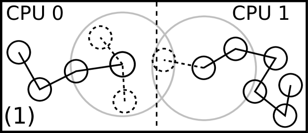
This algorithm ensures that each A or T particle can only participate in one new bond at each time step, even if several candidate bonds exist. This is achieved by selecting successively the pairs for a unique A and also for a unique T from the local and neighboring CPUs. This problem is illustrated in Fig. 1. The overall reaction rate depends naturally on the number of neighbor A T pairs in the system.

The effective bond formation is implemented by adding a bonded interaction term in the MD simulation. Explicitly, this amounts to call the add methods on the FixedPairList that contains the bonded Mirror Lennard-Jones interaction potential.

III.2 Current limitations

There are several possible extensions to the algorithm that would bring more generality. Taking into account several concurrent reactions is possible, following the Reactive multiparticle collision dynamics algorithm presented in Rohlf et al Rohlf et al. (2008) for collision-based hydrodynamical simulations. Further, the algorithm only considers irreversible reactions. Adding dissociation reactions would require an interaction potential that can be cut off without discontinuity. Quartic bonds have already been used for this purpose by Panico et al Tsige and Stevens (2004); Panico et al. (2010) in the LAMMPS Plimpton (1995) Molecular Dynamics simulation code.

IV Implementation in LAMMPS

IV.1 Existing implementation

LAMMPS provides officially the feature fix bond/create since january 2009 , although it may have been developed earlier as the use of the nearest partners is mentioned in Ref. Heine et al., 2004. As the details of the implementation of fix bond/create in LAMMPS have not been described in the literature, we review them here from the analysis of the file fix_bond_create.cpp. This fix operates at the post_integrate step in the MD integrator. LAMMPS does not possess a variable state for the particles. When a change is needed, it is done by modifying a particle’s type instead.

The parameters given to the fix bond/create command are: the types of the particles A and B, the cutoff distance for the bond creation, the bond type to create and optionally the maximum number of bonds to create for A and B, the type in which to transform A and B when reaching this maximum, a probability for the bond creation and the types of the angular and dihedral interactions to create.

As in the ESPResSo++ implementation, the algorithm relies on the existing neighbor list that is used for the non-bonded interactions.

1. For each neighbor pair that matches the types:

   1. Test for the correspondance of the types and the cutoff criterion.

   2. If the distance of the pair is lower than the minimum that was found previously, record the particles’ indices and distance.

2. The candidate pairs are consolidated among the processors using again the closest match in distance.

3. In each of the selected pairs, the evaluation of the reaction probability is done on the particle with the lowest identifier (the tag in LAMMPS). A random number in $[0,1)$ is compared to the user-defined probability.

This last criterion allows the choice of partners to be made uniquely in a simpler process than the one presented for ESPResSo++. The implication is that the choice of partners is not done at random among all possible partners. Parallel communications occur for the collection of partners and the synchronization of the random number assigned to each partner pair. A final communication ensures that the bond creation and type update is performed on each CPU.

After the bonds have been created, LAMMPS updates the connectivity of the system and checks for the generation of the angular and dihedral interactions that could result from the new molecular bonds, if the user has requested these in the fix bond/create instruction. Discontinuities in these interactions will perturb the trajectory and the energy of the system if enabled but remain a powerful feature to build atomistic networks.

The following considerations have to be considered when using fix bond/create. The user has to request the provision for extra connectivity information (i.e. allocation of appropriate storage for bonds, angles and dihedras, via the extra bond per atom and extra special per atom settings). We have included the repulsive Lennard-Jones potential, normally part of the nonbonded interactions, in the mirror Lennard-Jones bonded potential to follow the behaviour of the FENE bonds in LAMMPS. This is needed as bonded particles are excluded from the force evaluation, and this cannot be changed when the FENE potential is in use, which is the case here. The fix bond/create command keeps in memory the total number of bonds created during the simulation. If the user wishes to obtain further information on the bonds, e.g. on their distribution, it must be obtained via a dump to disk of the property nbond.

IV.2 New implementation

As will be seen in Sec. V, the existing algorithm in LAMMPS produces a different polymerization kinetics than the one we designed. To confirm that the difference originates in the selection algorithm, we implemented the algorithm presented in Sec. III in LAMMPS. To this end, we duplicated the code as fix bond/create/random and the code is available online de Buyl (2015b) under the GPL license version 2 that LAMMPS uses. The parallel communication routines are those provided by LAMMPS for fixes, into which we pack candidate lists for all the particles.

There is no state property in LAMMPS and the reaction is controlled by the number of bonds. As the initiation reaction for chain growth leaves the initiator with one bond while further reaction events leave the particles with two bonds we define the reaction twice:

$$\cee{P^{\ast}+M->[k]P-P^{\ast}}$$ (24)

and

$$\cee{P_{n-1}-P^{\ast}+M->[k]P_{n}-P^{\ast}}$$ (25)

where $P^{\ast}$ has a different type depending on whether it is already part of a chain or not.

V Simulations of chain growth

Simulations of chain growth start with $N_{P^{\ast}}$ P^∗ active units while the bulk of the simulation box is filled with monomer units M, for a total number of particles $N=N_{P^{\ast}}+N_{M}=10^{4}$, the initial number fraction of polymer is equal to the concentration of active sites

$$\phi_{0}=\frac{N_{P^{\ast}}}{N}$$ (26)

Table 2: Parameters used for the simulations. C1 and C2 are the single and multiple chains growth simulations, respectively. S are the step growth simulations. The species A and T are integer indices corresponding to the particles type in ESPResSo++. In LAMMPS the simulation parameters are the same. Besides A and T, we denote by A’ and T’ the integer types of A and T after reaction as there is no state variable. The maximum number of bonds allowed given to fix bond/create are also indicated.

ESPResSo++
Run	A	$\delta$A	$s_{min}^{A}$	T	$\delta$T	$k$	$\Theta$	$N_{tot}$
C1	0	-1	2	0	1	$1$, $0.1$ and $0.01$	10	$10000$
C2	0	-1	2	0	1	$0.1$	25	$10000$
S	1	-1	1	0	1	$0.1$ and $0.01$	25	13500

LAMMPS
	A	T	A’	T’	A max	T max
initiator	4	1	3	2	1	1
propagator	2	1	3	2	2	1
step	3	1	3	2	$f$	1

The number of particles in the states M, P and P^∗ is monitored for comparison with the rate equation. The resulting polymer fraction

$$\phi(t)=\frac{N_{P}+N_{P^{\ast}}}{N}$$ (27)

is then plotted for a proper comparison with the figures from Akkermans et al Akkermans et al. (1998).

To obtain numerical data for $\langle N_{P^{\ast}M}\rangle$, for different chain lengths, simulations of single chains are run in which the growth is stopped when the polymer chain reaches $n$ monomers. The integral of $g_{P^{\ast}M}(r)$ up to the cutoff radius is then used to obtain

$$\langle N_{P^{\ast}M}\rangle=\int_{0}^{r_{c}}4\pi r^{2}g_{P^{\ast}M}(r)dr~{}.$$ (28)

We observe a saturation of $\langle N_{P^{\ast}M}\rangle\approx 3.25$ with the chain length and use this limit value to compute $k_{c}$.

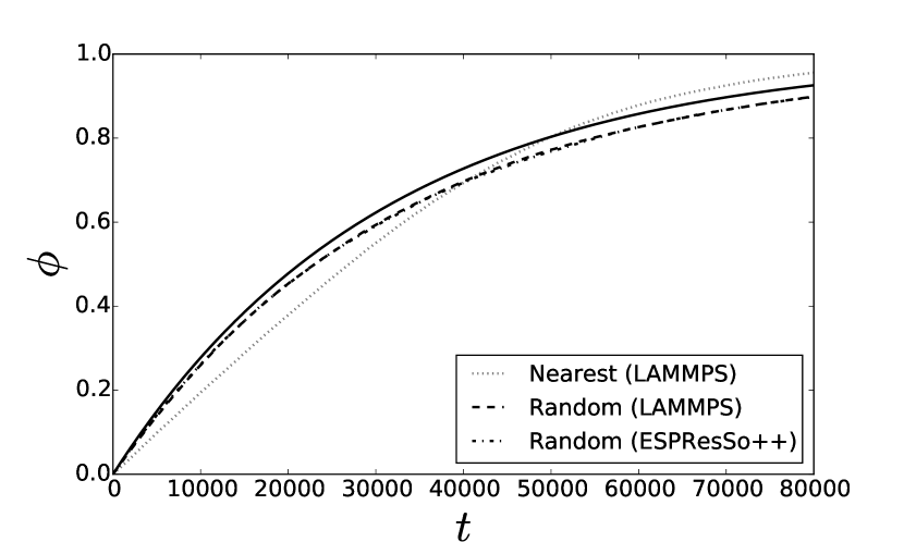
The first round of simulations, in Fig. 2 compares the algorithm in ESPResSo++ and in LAMMPS (existing and new). The existing algorithm in LAMMPS that selects the nearest partners for reaction does not follow the rate equation. To verify that difference arises from the reaction algorithm, we have re-implemented our algorithm in LAMMPS and obtain results that superimpose perfectly. Further simulations with LAMMPS only use this new algorithm.

Figure 2: Simulations of chain growth for the different algorithms. The full line is from Eq. (10). The random algorithm follows the theory albeit a little slowlier. The implementations in ESPResSo++ and LAMMPS are indistinguishable. The existing algoritm in LAMMPS (“Nearest”) does not follow the same kinetics and could not be fitted with an exponential function.

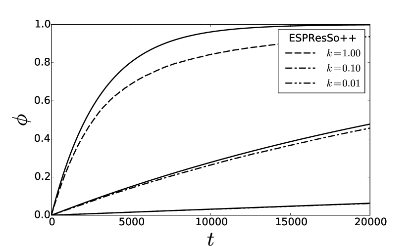
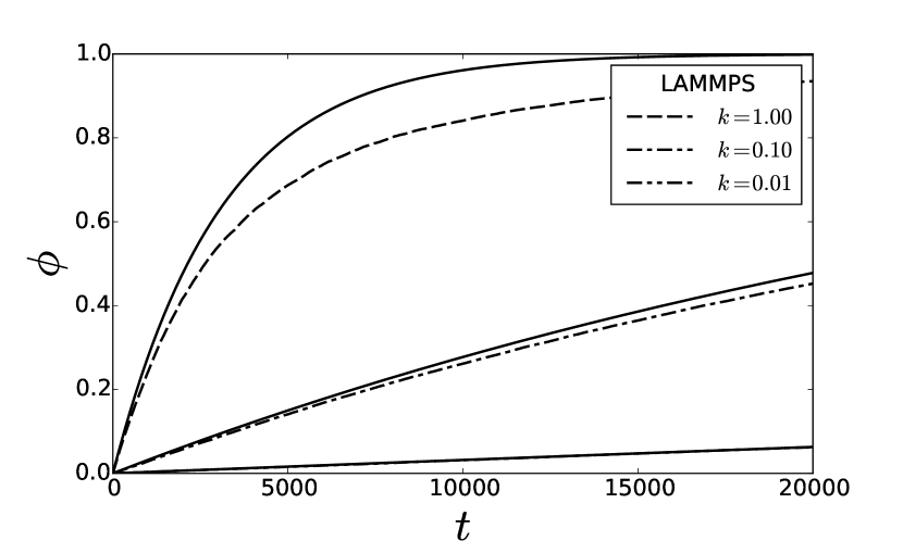
Further chain growth simulations were performed with a single chain, for different rates $k$, and are displayed in Fig. 3. As found by Akkermans et al Akkermans et al. (1998), the rate equation only compares well for low values of $k$. When the reaction rate is too high, the active end of the chain is not given enough time to find a new partner by molecular diffusion.

Figure 3: Simulations of chain growth (dash-dotted curves), for a single chain, for different intrinsic rates $k$ (see runs C1 of table 2 for the parameters). Each curve is the average over eight realizations. The full lines are the theoretical estimates for the corresponding effective rates from Eq. (10). For the fastest rate $k=1$ the theoretical estimates overestimates the monomer consumption rate, with respect to the simulation results. The discrepancy is reduced for $k=0.1$ and for the lowest value ($k=0.01$), the simulation results and the theory are undistiguishable.

To assess the behaviour of multiple chains growth, corresponding simulations have been run with initial polymer fractions $\phi_{0}$ of $1,3,5,10,15$ and $20~{}10^{-3}$. The resulting $\phi(t)$ is displayed as a fraction of the scaled time $k_{c}[P^{\ast}]t$ in Fig. 4.

Figure 4: Simulations of chain growth for multiple chains, for initial polymer fractions $\phi_{0}=1,3,5,10,15$ and $20~{}10^{-3}$ and rate $k=0.1$ (see runs C2 of table 2 for the parameters). The time is rescaled by the effective rate $k_{c}[P^{\ast}]$ so that the theoretical estimate (full line) matches all simulation data.

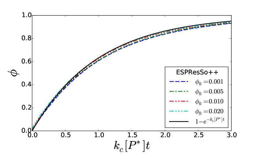
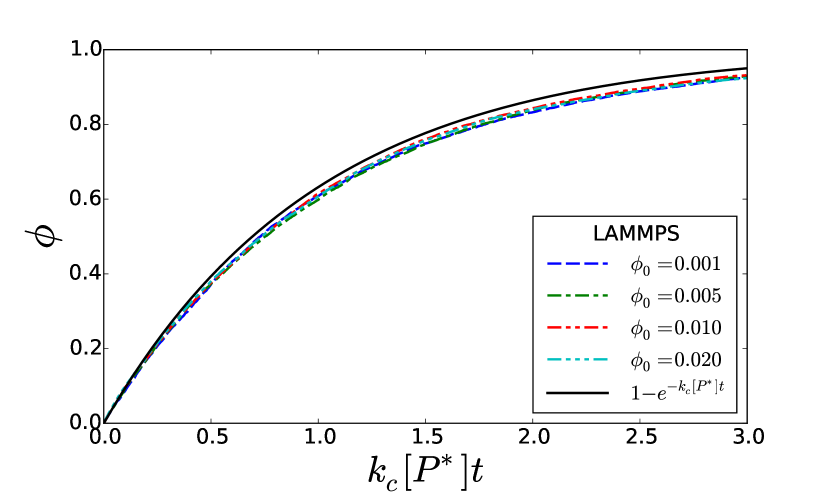
Given enough time, all chain growth simulations were observed to approach $\phi=1$, similarly to the limit of Eq. (10).

VI Simulations of step growth

We have performed simulations of step growth of a model system consisting of polymer chains $E-(P)_{n}-E$ with $n=3$, thus consisting of five monomer units, and of crosslinkers $X^{f}$. The simulations have been run with $f=0,1,2,3,4,5$ and rate $k=0.1$ and $0.1$ for a system of 2500 chains $E-(P)_{3}-E$ and 1000 crosslinkers $X$, for a total of 13500 particles in the system. These parameters give a stoechiometric ratio for $f=5$. They have been used for all values of $f$ to have only a single parameter vary across the simulations.

First, the radial distribution function $g_{X^{s}E^{0}}(r)$ between the crosslinker $X^{s\ast}$ and available end-unit $E^{0\ast}$ has been computed from simulations with $f=0,1,2,3,4$ and $5$, and $k=0.1$, where the polymerization runs for 5000 time units and is then stopped. The sampling for $g_{X^{s}E^{0}}(r)$ is done for 5000 subsequent time steps. The integral of $g_{X^{s}E^{0}}(r)$ up to the cutoff radius is then used to obtain

$$\langle N_{X^{s}E^{0}}\rangle=\int_{0}^{r_{c}}4\pi r^{2}g_{X^{s}E^{0}}(r)dr~{}.$$ (29)

The values of $\langle N_{X^{s}E^{0}}\rangle$ are given in Table 3 for reference.

$s$	0	1	2	3	4	5
$\langle N_{X^{s}E^{0}}\rangle$	1.30	0.890	0.572	0.327	0.137	1.28 10-2

Table 3: The average number of available neighbors for curing in the step-growth simulations.

Then, the polymerization has been studied in simulations where two rates have been used, $k=0.1$ and $0.01$ and the results are shown in Fig. 5.

Figure 5: Concentration of crosslinker states for the step-growth simulations with $f=1,2$ and $3$. The full black lines are obtained from Eqs. (14), and the dashed and dashed dotted lines come from simulations with $k=0.1$ and $k=0.01$, respectively. Each simulation result is the average over eight realizations. See the parameters for runs S in table 2. The curves starting at $x_{s}=1$ correspond to $x_{0}$. The curves starting at $x_{s}$ correspond $x_{s}$ with $s>0$, where the curves growing faster initially correspond to a lower $s$ (the fastest growing curve is for $s=1$, and so on). For $f=1$ and $2$, the rate equation captures properly the evolution of crosslinking. For higher functionalities, it fails to track the quantitative evolution beyond $kt\approx 1$ (see Fig. 6 for $f=4$ and $5$).

Figure 6: Same data as in Fig. 5 for $k=0.1$ and $f=4$ and $5$, with a logarithmic axis for the time (x-axis). The full black lines are obtained from Eqs. (14), and the grey lines come from simulations. Data is shown up to the end of the simulation, to highlight the saturation of $x_{5}$ (bottom panel) below the limiting value of $1$ that is reached for $f=4$ (top panel). Simulations performed with ESPResSo++.

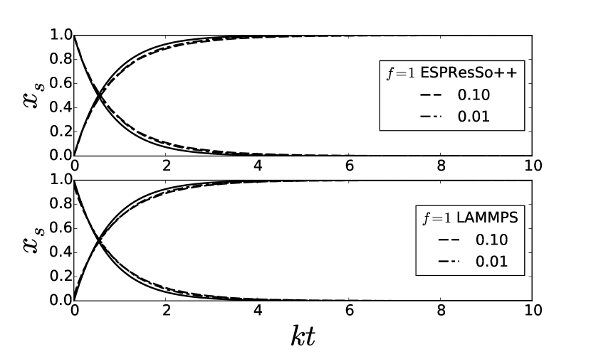
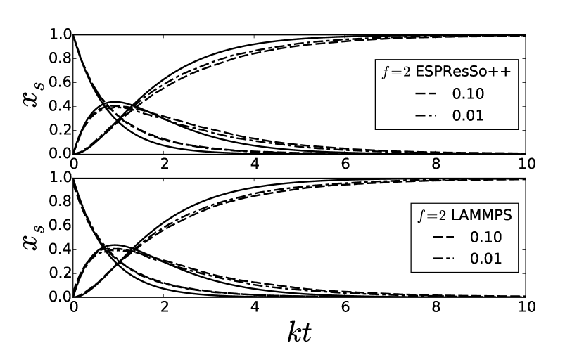
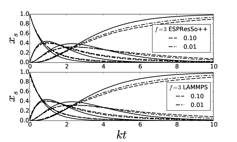
For low functionality ($f=1$ or $2$), the concentrations $[X^{s\ast}]$ given by Eqs. (14) compare well to the ones from the simulations. The simulation data shows a delay in the polymerization process, with respect to the rate equation, similarly to what has been observed for chain growth (see Sec. V). For higher functionality, the rate equation compares well to the simulation data only for the initial stages of the polymerization. Results for $kt$ up to $1.5$ are displayed to highlight the proper capture of the initial polymerization kinetics.

The discrepancy between the rate equation and the simulation data is unavoidable, as the rate equation only considers the average value for the number of reaction candidates, and highlights a motivation to develop the full simulation model.

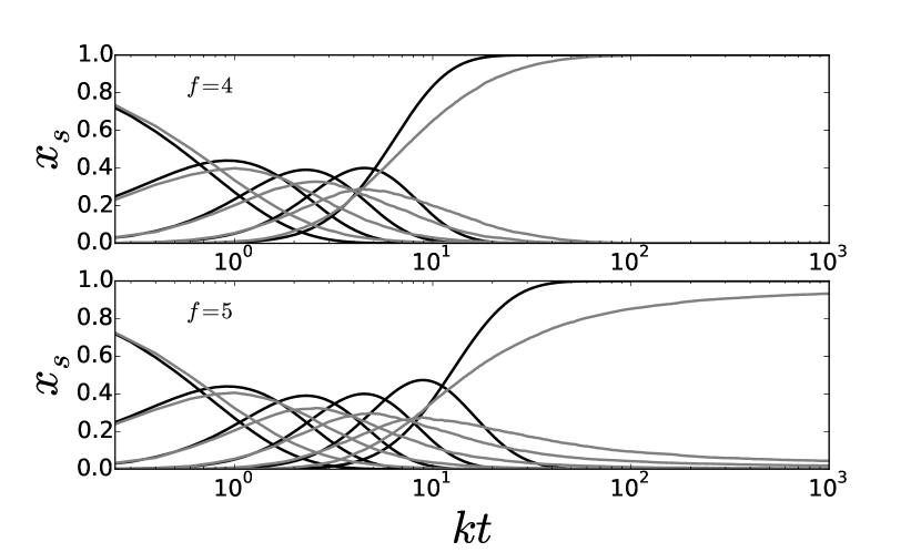
Figure 6 presents the same data as Fig. 5 with a larger time span (for $f=4$ and $f=5$ only). For $f=4$, the fraction $x_{4}$ of fully crosslinked X particles saturates at 1 (maximum value), similarly to the kinetic model. For $f=5$, besides the observed lag in the polymerization, we observe that $x_{5}$ does not reach the same saturation value. Indeed, crosslinkers having already formed four bonds (in the case $f=5$) have on average $0.01$ neighbours. This average hides the fact that many of these crosslinkers have zero neighbors of type and state E^0∗ that would allow further reaction. The polymerization is thus stopped by an effective depletion of reactant.

VII Conclusions

We have presented an adaptable algorithm for thermoneutral polymerization in parallel Molecular Dynamics (MD) simulations. The algorithm handles several polymerization mechanisms and may involve molecular compounds in which only selected sites participate in the polymerization process, as was done here for step growth. A difference in performance between ESPResSo++ and LAMMPS is observed, consistently with the observations made by the developers of ESPResSo++Halverson et al. (2013). Other criteria should guide the choice of the simulation package: the type of model simulated or the use of the Python interface, for instance.

The kinetic model of Akkermans et al Akkermans et al. (1998) was validated on the chain growth results and a kinetic model for step growth was introduced and compared favorably to the simulations. A systematic delay of the simulation process in the simulation is found for both growth mechanisms. That delay was also found in Refs. Akkermans et al., 1998; Hoy and Fredrickson, 2009 and is caused by the simplifications made in the rate equations with respect to the full molecular simulations. The polymerization algorithm has been implemented in ESPResSo++ and compared to the corresponding feature of LAMMPS. As a different kinetic evolution was found, we proceeded to implement our algorithm in LAMMPS to verify that this would bring the results in agreement, which was the case for chain growth and for step growth.

Due to the relative simplicity of coarse-grained models, with respect to atomistic descriptions, it is possible to control the polymerization process in its time evolution and to avoid typical artifacts such as energy jumps and discontinuous trajectories. On the basis of the present work, it is possible to backmap a system’s coordinates to the atomistic level after the polymerization process. Several extensions of the algorithm are feasible: introduce several concurrent chemical reactions with different intrinsic rates or further constrain the reaction acceptance to conformation properties (e.g. to avoid unrealistic angles in the newly formed molecule).

While the present work is limited to irreversible reactions, other works have already considered interaction potentials than “break” past a given cutoff Tsige and Stevens (2004). An alternative approach to the dissociation process is to consider a stochastic rate at which a bond dissapears Caby et al. (2012). This latter approach does not achieve energy conservation however. No solution that combines continuous trajectories and stochastic dissociation has been proposed yet.

Appendix A Simulation protocols in ESPResSo++ and LAMMPS

ESPResSo++ simulation protocol for chain and step growth:

1. Place particles at random in the simulation box. Chains for the step growth simulations are placed “one chain at a time” using the random-walk placement routine espresso.tools.topology.polymerRW of ESPResSo++.

2. Enable the velocity rescaling thermostat.

3. Run a warmup integration in which the interaction potential are capped at a maximum value.

4. Run a warmup integration in which the interaction potential are uncapped.

5. Disable the thermostat.

6. Run the “production” run, with the polymerization mechanism enabled.

LAMMPS simulation protocol for chain growth:

1. Place particles at random in the simulation box.

2. Enable the temp/rescale thermostat and use the nve/limit displacement limiter.

3. Run a warmup integration.

4. Disable the thermostat and displacement limiter.

5. Run the “production” run, with the polymerization mechanism enabled.

LAMMPS simulation protocol for step growth:

1. Replicate regularly a single chain in a low-density simulation box.

2. Place crosslinkers at random in the simulation box.

3. Enable the temp/rescale thermostat and use the nve/limit displacement limiter.

4. Iterate over MD runs and minimization steps.

5. Increase gradually the density to the target value with fix deform.

6. Disable the thermostat and displacement limiter.

7. Run a warmup integration with the nvt thermostat (Nosé-Hoover) at the target temperature.

8. Disable the thermostat.

9. Run the “production” run, with the polymerization mechanism enabled.

References

- Frenkel and Smit (2001) D. Frenkel and B. Smit, Understanding molecular simulation: from algorithms to applications (Academic press, 2001).
- Farah et al. (2012) K. Farah, F. Müller-Plathe, and M. C. Böhm, ChemPhysChem 13, 1127 (2012).
- Akkermans et al. (1998) R. L. C. Akkermans, S. Toxvaerd, and W. J. Briels, J. Chem. Phys. 109, 2929 (1998).
- Stevens (2001) M. J. Stevens, Macromolecules 34, 1411 (2001).
- Hoy and Fredrickson (2009) R. S. Hoy and G. H. Fredrickson, J. Chem. Phys. 131, 224902 (2009).
- Heine et al. (2004) D. R. Heine, G. S. Grest, C. D. Lorenz, M. Tsige, and M. J. Stevens, Macromolecules 37, 3857 (2004).
- Wu and Xu (2006) C. Wu and W. Xu, Polymer 47, 6004 (2006).
- Varshney et al. (2008) V. Varshney, S. S. Patnaik, A. K. Roy, and B. L. Farmer, Macromolecules 41, 6837 (2008).
- Plimpton (1995) S. Plimpton, J. Comput. Phys. 117, 1 (1995).
- Odegard et al. (2014) G. M. Odegard, B. D. Jensen, S. Gowtham, J. Wu, J. He, and Z. Zhang, Chem. Phys. Lett. 591, 175–178 (2014).
- van Duin et al. (2001) A. C. T. van Duin, S. Dasgupta, F. Lorant, and W. A. Goddard, The Journal of Physical Chemistry A 105, 9396 (2001).
- Halverson et al. (2013) J. D. Halverson, T. Brandes, O. Lenz, A. Arnold, S. Bevc, V. Starchenko, K. Kremer, T. Stuehn, and D. Reith, Comput. Phys. Commun. 184, 1129 (2013).
- de Buyl (2015a) P. de Buyl, “cg_md_polymerization,” http://dx.doi.org/10.5281/zenodo.15794 (2014-2015a).
- Mukherji and Abrams (2009) D. Mukherji and C. F. Abrams, Phys. Rev. E 79, 061802 (2009).
- Stevens (1999) M. P. Stevens, Polymer Chemistry (Oxford University Press, 1999).
- Jones et al. (01 ) E. Jones, T. Oliphant, P. Peterson, et al., “SciPy: Open source scientific tools for Python,” (2001–).
- de Buyl (2015b) P. de Buyl, https://github.com/pdebuyl/lammps/tree/fbc_random (2014-2015b).
- Kremer and Grest (1990) K. Kremer and G. S. Grest, J. Chem. Phys. 92, 5057 (1990).
- Rohlf et al. (2008) K. Rohlf, S. Fraser, and R. Kapral, Comput. Phys. Commun. 179, 132 (2008).
- Tsige and Stevens (2004) M. Tsige and M. J. Stevens, Macromolecules 37, 630 (2004).
- Panico et al. (2010) M. Panico, S. Narayanan, and L. C. Brinson, Modelling Simul. Mater. Sci. Eng. 18, 055005 (2010).
- Note (1) http://lammps.sandia.gov/history.html.
- Caby et al. (2012) M. Caby, P. Hardas, S. Ramachandran, and J.-P. Ryckaert, J. Chem. Phys. 136, 114901 (2012).