Exploiting Non-Markovianity of the Environment for Quantum Control

Abstract

When the environment of an open quantum system is non-Markovian, amplitude and phase flow not only from the system into the environment but also back. Here we show that this feature can be exploited to carry out quantum control tasks that could not be realized if the system was isolated. Inspired by recent experiments on superconducting phase circuits, we consider an anharmonic ladder with resonant amplitude control only. This restricts realizable operations to SO(N). The ladder is immersed in an environment of two-level systems. Strongly coupled two-level systems lead to non-Markovian effects, whereas the weakly coupled ones result in single-exponential decay. Presence of the environment allows for implementing diagonal unitaries that, together with SO(N), yield the full group SU(N). Using optimal control theory, we obtain errors that are solely $T_{1}$-limited.

Quantum control, employing external fields to steer the outcome of a dynamical process Rice and Zhao (2000); Brumer and Shapiro (2003), holds the promise of utilizing entanglement and matter interference as cornerstones of future technologies. Accurate and reliable control solutions may be identified by optimal control, provided the control target is reachable. This question is addressed by controllability analysis. For closed quantum systems, the answer is determined solely by symmetries in the Hamiltonian and the available resources such as power or bandwidth of the controls D’Alessandro (2007). Controllability and control strategies for non-Markovian open quantum systems remain largely uncharted territory. Non-Markovianity refers to memory effects in the environment and the built-up of non-negligible correlations between system and environment Breuer (2012). It is generic for condensed phase settings encountered e.g. in light harvesting or solid-state devices. Non-Markovianity can be measured in terms of information flowing from the environment back into the system Breuer et al. (2009), increase of correlations if the system is bi- or multipartite Rivas et al. (2010), or re-expansion of the volume of accessible states in Liouville space Lorenzo et al. (2013). Each of these measures holds a promise for improved control for non-Markovian compared to Markovian open systems: Partial recovery of coherence or growth of correlations or a larger accessible state space volume should all clearly facilitate control. Indeed, correlations between system and environment may improve fidelities of single qubit gates Rebentrost et al. (2009), cooperative effects of control and dissipation may allow for entropy export and thus cooling Schmidt et al. (2011), and harnessing non-Markovianity may enhance the efficiency of quantum information processing and communication Laine et al. (2014); Bylicka et al. (2014).

Here, we go beyond merely improving a given figure of merit and show that a non-Markovian environment may enable the implementation of quantum operations that could not be realized without presence of the environment. Our approach is based on separating the environment into potentially beneficial and potentially detrimental parts, with the latter setting the timescale for (almost) unitary operations. We employ optimal control theory (OCT) to best exploit the beneficial non-Markovian part of the environment while beating decoherence due to the detrimental Markovian part. For a four-level anharmonic ladder system with resonant amplitude control only, which by itself is SO(4)-controllable, we demonstrate that full SU(4)-controllability can be achieved due to the presence of the environment. The fidelities are only limited by the Markovian decay.

We investigate quantum control for a four-level system since analytical solutions to the problem of population inversions can be obtained by Pythagorean coupling Suchowski et al. (2011) which allow for realizing arbitrary operations in SO(4). A recent experimental demonstration employed resonant amplitude control in a flux-biased Josephson phase circuit Svetitsky et al. (2014). The simplest way to construct an arbitrary element of SU(N), provided that one is able to implement any element of SO(N), is obtained by the Cartan decomposition. It results in a decomposition of all unitaries $U\in\,$SU(N) into local operations, $k_{1},k_{2}\in\,$SO(N), and a diagonal, unitary matrix $A$ such that $U=k_{1}Ak_{2}$ D’Alessandro (2007). The task to achieve full unitary controllability on the $N$-level system therefore reduces to implementing an arbitrary diagonal unitary. This is the problem we address in the following, employing OCT.

We consider an anharmonic $N$-level system that interacts, possibly strongly, with an environment. This interaction leads to (i) pure dephasing due to long-time memory, low-frequency noise; (ii) energy relaxation due to weakly coupled near-resonant environmental nodes; and (iii) visible splittings in the systems’s energy levels due to strongly coupled near-resonant environmental nodes. The strongly coupled modes are best accounted for explicitly (”primary bath”), and we assume here that they can be modeled by two-level systems (TLS) Baer and Kosloff (1997); Koch et al. (2002); Gelman et al. (2004); Gualdi and Koch (2013). Both $N$-level system and primary bath are weakly coupled to a thermal reservoir (”secondary bath”) to account for effects (i) and (ii) . This is modelled by a Markovian master equation ($\hbar=1$) for the joint state of system (”Q”) and primary bath (”P”),

$$\frac{d\rho_{QP}}{dt}=-i[H_{QP},\rho_{QP}]+\mathcal{L}_{S}(\rho_{QP})\,,$$ (1)

with the Hamiltonian $H_{QP}$ generating the coherent evolution and the Liouvillian $\mathcal{L}_{S}$ capturing the effect of the secondary bath (”S”). The state of the system alone, $\rho_{Q}$, is obtained by integrating over the primary bath modes Baer and Kosloff (1997); Koch et al. (2002) that can give rise to non-Markovian effects. For $n_{P}$ TLS in the primary bath, $H_{QP}$ reads

$$H_{QP}=H_{Q}+\sum_{i=1}^{n_{P}}H^{(i)}_{P}+\sum_{i=1}^{n_{P}}H_{int}^{(i)}\,,$$ (2)

with $H_{Q}$ describing an anharmonic ladder, $E_{n}=n\omega_{Q}+\beta n(n+1)/2$, with base frequency $\omega_{Q}$ and anharmonicity $\beta$ plus control by an external field. The $i$th TLS is characterized by the splitting $\omega_{i}$, $H^{(i)}_{P}=\omega_{i}\sigma^{z}_{i}$, and couples transversally to the $N$-level system,

$$H_{int}^{(i)}=\frac{S^{(i)}}{2}\left(a\sigma_{i}^{+}+a^{\dagger}\sigma_{i}^{-}\right)\,,$$ (3)

with $a^{+}$ ($a$) the creation (annihilation) operator of the $N$-level system, and the coupling constant $S^{(i)}$ corresponding to the system’s energy level splitting when on resonance with the $i$th TLS. The Liouvillian models decay of system and primary bath,

$$\mathcal{L}_{S}(\rho)=\sum_{k}\left(A_{k}\rho A_{k}^{\dagger}-\frac{1}{2}\left[A_{k}^{\dagger}A_{k},\rho\right]_{+}\right)\,,$$ (4)

with $A_{n}=\sqrt{n/T_{1}}\Ket{n-1}\Bra{n}$ and $A_{i}=\sqrt{1/T_{1}^{(i)}}\sigma_{i}^{-}$. In order to limit the number of parameters, we restrict our model to a $T_{1}$-limited environment. We have verified that it effectively captures both loss and dephasing, i.e., adding pure dephasing characterized by $T_{2}^{*}$ behaves, in terms of the final fidelities, similarly to Eq. (4) with increased $T_{1}$. A good realization of this model is given by superconducting circuits where the TLS correspond to dielectric defects Martinis et al. (2005) and the thermal bath can be taken at $T=0\,$K . In particular, the TLS can be characterized experimentally in terms of their splitting, coupling to the $N$-level system, and $T_{1}$ Shalibo et al. (2010); Shalibo (2012); and the upper bound of modelling both Markovian loss and pure dephasing by an effective $T_{1}$ becomes tight since $T_{2}$ is typically close to $T_{2}^{*}$ Barends et al. (2013).

The $N$-level system is subjected to an external control $u(t)$ that shifts its energy levels. This can be achieved, for example, by low-frequency steering of the bias flux in phase qudits Shalibo (2012). For low anharmonicity, the shift is harmonic,

$$H_{c}\left[u(t)\right]=\sum_{n=0}^{N-1}u(t)\;n\omega_{Q}\Ket{n}\Bra{n}\,.$$ (5)

In case of the bias flux on the phase qudit, this corresponds to neglecting terms that oscillate strongly on the timescale of $\omega_{Q}$. It is those terms that, for $N=4$, yield SO(4) operations via the Pythagorean coupling Svetitsky et al. (2014). Consequently, the two control mechanisms, high-frequency steering on the one hand and low-frequency steering on the other, do not interfere. Moreover, our low-frequency control does not induce transitions to levels with $n>4$ since all operators in the Hamiltonian (2) conserve the occupation number of the joint state of system and primary bath.

In the absence of the primary bath, the control Hamiltonian (5) does not allow for realizing arbitrary diagonal unitaries in the four-level subspace. This is best analyzed in terms of the dynamic Lie algebra. It represents the Hilbert space directions along which the system can evolve and is formed by nested commutators of control and drift Hamiltonian. Since $H_{c}$ and $H_{Q}$ commute, evolution along only a single direction is possible. The scenario changes once the strongly coupled TLS of the primary bath come into play. In fact, a single strongly coupled TLS is sufficient to provide the remaining $N-1$ Hilbert space directions, required for realizing an arbitrary diagonal unitary. This is due to $H_{c}$ not commuting with $H_{int}^{(i)}$. In more physical terms, $H_{int}^{(i)}$ allows for the system wave function to be transferred to the TLS and back, after acquiring the desired non-local phases.

These considerations of controllability hold, however, only for unitary evolution. The secondary bath leads to irreversible loss of energy and phase of both system and primary bath TLS. The only control strategy that is available for such Markovian dynamics is to beat decoherence (unless a protected region in Hilbert space exists in which the desired dynamics can be generated). It is thus crucial to carry out all operations as fast as possible. Since OCT allows for identifying controls that operate at the speed limit Goerz et al. (2011), we use it here, employing a recent variant for unitary gates in open quantum systems Goerz et al. (2014). Our optimization target is $U_{1}=\mathrm{diag}(1,-1,1,1)$, and we quantify success in terms of the error, $1-F_{average}$ Nielsen and Chuang (2000). $U_{1}$ is a particularly difficult unitary to implement, as exemplified by an error of over 40% in the absence of any strongly coupled TLS. While we discuss in the following only $U_{1}$, we have verified that optimization towards diagonal unitaries with random phases yield very similar errors . This suggests full SU(4)-controllability, once implementation of $U_{1}$ is successful.

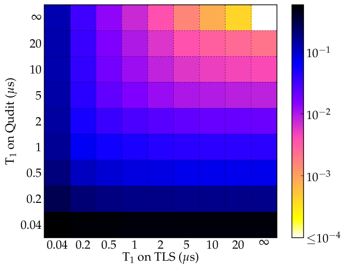
Figure 1: (color online) Error after optimization for $\mathrm{diag}(1,-1,1,1)$ as a function of $T_{1}$ times of qudit and TLS for an optimization time of $T=40\,$ns (anharmonicity $\beta=40\,$MHz, $\omega_{Q}-\omega^{(1)}=550\,$MHz, $S^{(1)}=60\,$MHz).

Figure 1 demonstrates the interplay of Markovian and non-Markovian effects by plotting the error for $U_{1}$ as a function of the $T_{1}$ times of qudit and one TLS: Errors below 1% can be reached even for $T_{1}$ times of the order of a few microseconds. Due to increasing decoherence rate with increasing excitation, short $T_{1}$ times of the qudit have a slightly more severe effect than short $T_{1}$ times of the TLS. A multitude of controls lead to the results shown in Fig. 1. Two examples of optimized controls, obtained using different constraints, are displayed in Fig. 2(a):

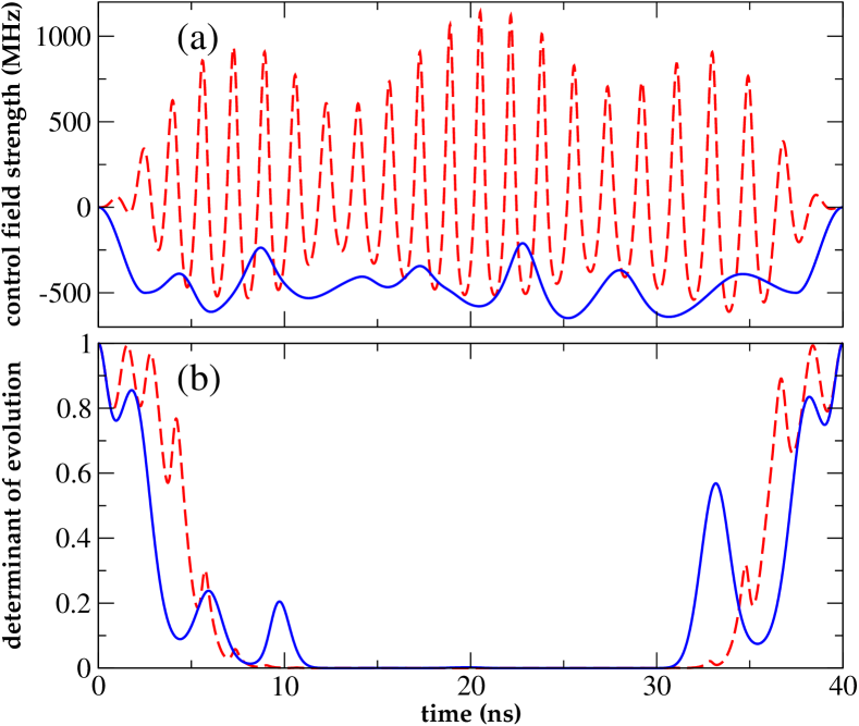
Figure 2: (color online) (a): Optimized amplitudes with the control shown in blue following a fixed ramp of $\pm 500\,$MHz over $2.5\,$ns at the beginning and end and the red dashed line obtained without imposing a ramp. (b): Liouville space determinant of the system evolution – increase of the determinant indicates non-Markovianity.

The control can be restricted to low bandwidth by ramping it into and out of resonance at the beginning and end of the optimization time interval (blue solid line in Fig. 2(a)), whereas fast oscillating controls are obtained without imposing a ramp (red dashed line in Fig. 2(a)). The different controls all share the mechanism of moving the qudit close to resonance with the TLS, picking up a non-local phase due to the enhanced interaction, and moving the qudit back off resonance. This sequence is repeated several times in order to properly align all the phases in the four-level subspace. A visualization of the dynamics is provided as supplementary material. While both controls lead to similar errors, the ramped control is easier to implement experimentally and also fulfills the low-frequency approximation used to derive the control Hamiltonian (5). All further calculations therefore employ ramped controls. Both solutions shown in Fig. 2(a) use non-Markovianity of the time evolution as core resource for control. This is seen in Fig. 2(b) which plots the determinant of the volume of reachable system states Lorenzo et al. (2013), a non-Markovianity measure that is easily evaluated numerically: Any increase in the determinant indicates non-Markovianity.

Use of the environment as a resource is further illustrated in Fig. 3 which explores the dependence of the best possible error on qudit anharmonicity and coupling strength between qudit and TLS: For very small coupling no solution can be found and the error remains of the order one.

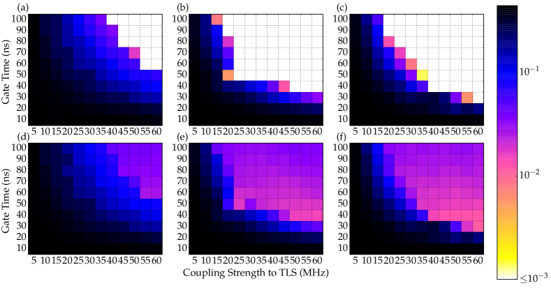
Figure 3: (color online) Error after optimization for $\mathrm{diag}(1,-1,1,1)$ for three different anharmonicities, $\beta=0\,$MHz (a,d), $40\,$MHz (b,e), $150\,$MHz (c,f) and infinite $T_{1}$ of both qudit and TLS (a-c) vs realistic $T_{1}$ (d-f, $T_{1}=5\,\mu$s (qudit), $T^{(1)}_{1}=1\,\mu$s (TLS)).

On the other hand, a single, only moderately coupled TLS in the primary bath is sufficient to yield good fidelities even for weak or zero anharmonicity. In the latter case (Fig. 3(a,d)), the desired diagonal unitaries can be realized if the operation time is sufficiently long. This can only be exploited for good $T_{1}$ times, utilizing the level-dependent coupling strengths. The control problem becomes much easier for non-zero anharmonicity, with a subtle interplay between the requirements of resolving the qudit levels and sufficient interaction with all qudit levels. The latter corresponds to small anharmonicity (Fig. 3(b,e)) and subsequently allows good results even for weak coupling, whereas energy resolution is best for larger anharmonicity (Fig. 3(c,f)), which in turn allows for very short operation times. For fixed anharmonicity, one expects larger coupling strengths and longer gate times to allow for better fidelities. A few exceptions to this rule, which are observed in Fig. 3, can be attributed to the numerical nature of our controllability analysis. The observation that for a very weakly coupled TLS there exists no anharmonicity and no gate time that lead to even moderate fidelities is clear evidence that the primary bath TLS is essential for the generation of arbitrary diagonal unitaries.

$\Delta^{(2)}$	$S^{(2)}$	$T^{(2)}_{1}$	error
50 MHz	40 MHz	2000 ns	$3.076\cdot 10^{-2}$
50 MHz	40 MHz	200 ns	$4.052\cdot 10^{-2}$
50 MHz	40 MHz	40 ns	$7.867\cdot 10^{-2}$
50 MHz	10 MHz	2000 ns	$3.196\cdot 10^{-2}$
50 MHz	10 MHz	200 ns	$3.564\cdot 10^{-2}$
50 MHz	10 MHz	40 ns	$4.241\cdot 10^{-2}$
450 MHz	40 MHz	2000 ns	$1.659\cdot 10^{-2}$
450 MHz	40 MHz	200 ns	$1.652\cdot 10^{-2}$
450 MHz	40 MHz	40 ns	$1.758\cdot 10^{-2}$
450 MHz	10 MHz	2000 ns	$1.663\cdot 10^{-2}$
450 MHz	10 MHz	200 ns	$1.674\cdot 10^{-2}$
450 MHz	10 MHz	40 ns	$1.675\cdot 10^{-2}$

Table 1: Error after optimization for $\mathrm{diag}(1,-1,1,1)$ with two primary bath TLS (parameters for qudit and first TLS as in Fig. 2, second TLS positioned $\Delta^{(2)}$ below $\omega^{(1)}$). For comparison, the error obtained for a single TLS is $1.652\cdot 10^{-2}$.

While the primary bath may provide interactions with the system that can be used as a resource for control, it can also have detrimental effects on the system, in particular when more than one TLS comes into play. This is likely to happen since number, position and coupling strength of the TLS cannot be controlled in the preparation of the actual devices. We therefore analyze the presence of an additional primary bath TLS in our optimizations, cf. Table 1. If the TLS are not too close to each other, a suitable control can suppress the effect of the additional TLS even if it is strongly coupled and very noisy. On the other hand, and not surprisingly so, the stronger a closely lying second TLS is coupled to the qudit, the more difficult it is to maintain good fidelities. This is due to the fact that the gate time needs to be sufficiently long to resolve the energy difference between the two TLS. Adding more TLS to the primary bath does not change the picture shown in Table 1: In optimizations with as many as four strongly coupled primary bath TLS, the error is increased by less than a factor of 2 compared to the error for a single TLS if none of the additional TLS is close to the favourable one and less than a factor of 4 if a moderately lossy TLS is in its vicinity.

In summary, we have shown that a non-Markovian environment can be exploited for quantum control, enabling realization of all quantum operations in SU(4) where the system alone allows only for SO(4). The enhanced controllability results from an effective control over the system-bath coupling by moving the system into and out of resonance with a selected bath mode. Fast implementations of this control scheme were obtained with OCT such that the errors are solely $T_{1}$-limited. Our model and results are directly applicable to superconducting phase and transmon circuits for which we predict, with reasonably simple controls, errors below one per cent for state of the art decoherence times.

More generally, our results provide a new perspective on open quantum systems – the environment can act as a resource for (almost) unitary quantum control which can be exploited using OCT to get the details of the dynamics right. It requires one or a few environmental modes to be sufficiently isolated and sufficiently strongly coupled to the system. These conditions are met for a variety of solid-state devices other than superconducting circuits, for example NV centers in nanodiamonds or nanomechanical oscillators. In addition, on an abstract level, our work calls for a comprehensive investigation of controllability of open quantum systems, in order to gain a rigorous understanding of when and how non-Markovianity is beneficial for quantum control.