Scaling laws for the bifurcation-escape rate in a nanomechanical resonator

Abstract

We report on experimental and theoretical studies of the fluctuation-induced escape time from a metastable state of a nanomechanical Duffing resonator in cryogenic environment. By tuning in situ the non-linear coefficient $\gamma$ we could explore a wide range of the parameter space around the bifurcation point, where the metastable state becomes unstable. We measured in a relaxation process the distribution of the escape times. We have been able to verify its exponential distribution and extract the escape rate $\Gamma$. We investigated the scaling of $\Gamma$ with respect to the distance to the bifurcation point and $\gamma$, finding an unprecedented quantitative agreement with the theoretical description of the stochastic problem. Simple power scaling laws turn out to hold in a large region of the parameter’s space, as anticipated by recent theoretical predictions. These unique findings, implemented in a model dynamical system, are relevant to all systems experiencing under-damped saddle-node bifurcation.

Transition from a metastable to a stable state is a phenomenon of ubiquitous interest in science: in thermal equilibrium it is the essence of the activation law in chemistry Arrhenius (1889); Kramers (1940), it underlies nucleation in phase transitions, magnetization reversal in molecular magnets Novak et al. (1995), biological switches in cells behavior Ozbudak et al. (2004) or RNA dynamics Dethoff et al. (2012), transitions of Josephson junctions Turlot et al. (1989) or fluctuations in SQUIDs Kurkijärvi (1972), the list being obviously non-exhaustive. More recently the study of escape statistics has been possible also for out-of-equilibrium dynamical systems like Penning traps Lapidus et al. (1999), Josephson junctions Siddiqi et al. (2004), and nano-electromechanical systems Aldridge and Cleland (2005); Stambaugh and Chan (2006); Chan and Stambaugh (2007); Chan et al. (2008); Unterreithmeier et al. (2010): the state-switching effect is extensively used in bifurcation amplifiers, with for instance state-of-the-art quantum bit readout schemes Boulant et al. (2007). In most of these cases the escape time distribution is exponential and the rate $\Gamma$ characterizes completely the phenomenon. Analytical solutions Hänggi et al. (1990) of the dynamical equations show that its value depends exponentially on a parameter $D^{-1}$, that coincides with the (inverse of the) temperature for equilibrium systems and more generally is related to the power spectrum of the relevant fluctuations. One can then write:

$$\Gamma=\Gamma_{0}\exp(-E_{a}/D),$$ (1)

where the prefactor $\Gamma_{0}$ is assumed to depend very weakly on $D$, and $E_{a}$ in analogy with a potential system can be called activation energy: it parametrizes the distance to the unstable point. For out-of-equilibrium systems a central theoretical result is the paper by Dykman and Krivoglaz Dykman and Krivoglaz (1979), that found an explicit expression for $E_{a}$ and $\Gamma_{0}$ for a generic dynamical system close to the bifurcation point, where the line of metastable states joins the line of unstable ones. It predicts universal power laws dependence of $E_{a}$ and $\Gamma_{0}$ on the distance from the bifurcation point in terms of $|\omega-\omega_{b}|$, where $\omega$ is the driving frequency of the dynamical system and $\omega_{b}$ is its bifurcation value.

Direct experimental measurement of the escape time and study of the dependence of $E_{a}$ and $\Gamma_{0}$ over a wide range of a system’s parameters is not a trivial task, since the exponential dependence of the escape time makes it either too long or too short for a reasonable observation protocol. For dynamical systems the resonating period fixes a lower bound on the time. Nano-mechanical resonators with resonance frequency in the MHz range are thus a prominent choice to investigate the bifurcation instability of Duffing oscillators: they are high frequency dynamical systems with a high quality factor for which the distance to the bifurcation point can be directly controlled.

In the analysis of switching and reaction rates, three problems can thus be distinguished: obtaining the exponent $E_{a}$, the prefactor $\Gamma_{0}$, and their respective scalings for systems away from thermal equilibrium. The exponent has been the first subject of interest, with the early work of Arrhenius Arrhenius (1889). The prefactor has then been addressed by Kramers later on Kramers (1940), while finally the scaling of both for dynamical systems has been derived by Dykman Dykman and Krivoglaz (1979). It is actually in micro and nano-mechanical systems that a measurement of the power law dependence of $E_{a}$ with respect to the distance from the bifurcation point has been performed, giving the predicted value within experimental error Aldridge and Cleland (2005); Stambaugh and Chan (2006). Nevertheless, the activation energy has been claimed to match theory at best within a factor of 2 due to injected noise calibration Aldridge and Cleland (2005). To our knowledge no attempts have been done to obtain a more quantitative verification of the predictions of Dykman and Krivoglaz Dykman and Krivoglaz (1979), in particular for the scaling law of the prefactor $\Gamma_{0}$ and the dependence to the Duffing non-linear coefficient $\gamma$ of both $\Gamma_{0}$ and $E_{a}$. Answering the three above mentioned problems together is thus the aim of our work, using a unique nano-mechanical implementation of the bifurcation phenomenon.

In this Letter we report on experimental and theoretical investigations of the dependence of $E_{a}$ and $\Gamma_{0}$ on the system parameters for a driven nano-mechanical oscillator in the non-linear regime in presence of a controlled noise force. It is well known that for a sufficiently strong non-linear term the system admits for some values of the driving frequency a metastable solution. By measuring the escape rate for a wide range of parameters we could verify the validity of the power scaling laws predicted by Dykman and Krivoglaz for both $E_{a}$ and $\Gamma_{0}$. Remarkably, we found that the scaling holds experimentally in a much larger region of the parameter space than the one for which the theory of Ref. Dykman and Krivoglaz (1979) has been derived. Concerning the $E_{a}$ dependence on detuning, the possibility of an extended region of scaling was discussed in Refs. Dykman et al. (2005); Kogan (2008). Performing the full numerical simulation of the stochastic problem adapted to our device parameters we found that experiment and theory are in excellent quantitative agreement.

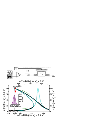
Figure 1: (Color online) Top panel: Schematic of the experimental setup with the nano-resonator structure. Bottom panel: Linear and Duffing resonances (respectively grey and black points, with top-right and bottom-left axes). The lines show the fit. The nonlinear resonance is for $V_{g}$ = 9.4 V, which shifts the resonance frequency and opens an hysteresis (thin green arrows highlight upward and downward sweeps). The relaxations occur at a detuning $\omega-\omega_{b}$ from the bifurcation frequency (red point and vertical arrow). Inset: Gaussian distribution histogram of the measured intrinsic frequency fluctuations.

The experiment is performed on a unique goalpost (depicted in top graph of Fig. 1) aluminum-coated silicon nano-electro-mechanical resonator. It consists in two cantilever feet of length 3 $\mu$m linked by a paddle of length 7 $\mu$m, all about 250 nm wide and 150 nm thick for a total mass $m=$ 1.25 $10^{-15}$ kg Collin et al. (2012). The experiment is performed at $4.2$ K in cryogenic vacuum (pressure$~{}<10^{-6}$ mbar). The motion is actuated and detected by means of the magnetomotive scheme Cleland and Roukes (1999), with a magnetic field $B<1$ T and a gate electrode is also capacitively coupled to the nanomechanical device (gap about 100 nm) Collin et al. (2012). The resonator admits large distortions (in the hundred nm range) to be attained while remaining intrinsically extremely linear Collin et al. (2011a), while a well-controlled non-linearity can be generated by means of a DC gate voltage bias $V_{g}$ Kozinsky et al. (2006). This distinctive feature enables to tune the global non-linearity of our device without changing the displacement amplitude. Using an adder we apply both a sinusoidal drive and a noise voltage from a voltage source generator. The resulting electric signal together with a 1 kOhm bias resistor is used to inject an AC current through the goalpost and generates both driving and controllable (zero average) noise forces on the resonator. More information on the calibration and experimental details can be found in Refs. Collin et al. (2011a, 2012). The resulting equation of motion for the resonator displacement $x$ reads:

$$\ddot{x}+\Delta\omega\dot{x}+\omega_{0}^{2}x+\gamma x^{3}=f_{d}\cos(\omega t)+f_{n}(t)$$ (2)

with $\omega_{0}/2\pi$=7.07 MHz the resonance frequency, $\Delta\omega/2\pi$=1.84 kHz the linewidth, and $f_{d}$ and $f_{n}$ the drive and noise forces divided by the mass of the resonator. We fix the drive force so that $mf_{d}~{}$= 65 pN, leading to a constant maximal displacement amplitude of 100 nm. As can be deduced from our characterizations Collin et al. (2012), this amplitude is small enough to guarantee that nonlinear damping mechanisms such as discussed in Refs. Zaitsev et al. (2012); Collin et al. (2011b) are small (see comment in the discussion section). The noise force signal is filtered so that the force spectrum $\int dte^{i\omega t}\langle f_{n}(t)f_{n}(0)\rangle_{\omega}=2D$ is constant over a bandwidth of 1 MHz around 7 MHz. The Duffing coefficient $\gamma$ scales as $V_{g}^{2}$ and is for us negative Collin et al. (2011a). At fixed driving force, the system admits two amplitudes of oscillation for sufficiently large $|\gamma|$ as shown in Fig. 1 (bistability). By fitting with the standard Duffing expressions Collin et al. (2010) the parameters $\Delta\omega$, $\omega_{0}$ and $\gamma$ together with the bifurcation frequency $\omega_{b}$ can be obtained with a good accuracy. The experiment is then performed by sweeping $\omega$ from the stable regime ($\omega>\omega_{0}$) down to the edge of the hysteresis at a given value of $\omega-\omega_{b}$ in the high amplitude state (see Fig. 1). The sweeping rate (a few Hz/s) is an important parameter which should both guarantee adiabaticity of the sweep and high accuracy in the measurement . Finally, the escape time from the metastable state is detected when the measured displacement amplitude falls below an appropriate threshold value. Typically $10^{3}$ escape events are recorded for each set of parameters. The experiment has been repeated for three different values of the noise forces $f_{n}$, three different detunings $\omega-\omega_{b}$ (up to 5$\%$ of the hysteresis), and five different values of $V_{g}$ (and thus of $\gamma$), for a total of 45 escape histograms. The resulting settings are summarized in Fig. 2.

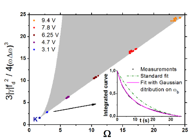
Figure 2: (Color online) Bifurcation parameter space (normalized driving force versus $\Omega=2|\omega-\omega_{0}|/\Delta\omega$). The grey area is the NEMS bistability regime where the right edge is the transition from a high amplitude oscillation to a low one (the left edge is the opposite) and K is the spinode point where hysteresis starts to open. We show within the bistability the data points at different voltages $V_{g}$. Inset: typical low $V_{g}$ relaxation curve obtained with about 1000 relaxations, and fit with and without fluctuations on $\omega_{b}$.

For each data measurement, the experimental value of $\omega_{b}$ might slightly differ from the one obtained by the initial fit. This problem is detected by sweeping relatively rapidly $\omega$ (tens of Hz/sec) through the bifurcation point and measuring the escape value $\omega_{b}$ prior to each relaxation-time acquisition. A typical histogram of the distribution of $\omega_{b}$ is shown in the inset of Fig. 1 for $V_{g}=9.4~{}$V. It has Gaussian form with a half-width $\sigma$ in the range of tens of Hz. This tiny spread ($10^{-6}$ to $10^{-5}$ of $\omega_{b}$) is due to low-frequency intrinsic fluctuations of the resonating frequency, which actual origin is still under debate Fong et al. (2012); Zhang et al. (2014); van Leeuwen et al. (2014). Even if extremely small, due to the high sensitivity of the bifurcation phenomenon the fluctuations of $\omega_{b}$ modify slightly the value of $\Gamma$ at each measurement, and we have to take this effect into account. The escape exponential distribution has thus to be averaged over these fluctuations. For $|\omega-\omega_{b}|\gg\sigma$ one can expand this dependence: $\Gamma(\omega-\omega_{b}-\epsilon)=\Gamma+\Gamma^{\prime}\epsilon+\dots$, where $\epsilon$ is the Gaussian-distributed shift of $\omega_{b}$. This gives the following distribution for the escape times:

$$P(t)=\Gamma e^{-\Gamma t}\int{d\epsilon\over\sigma\sqrt{2\pi}}e^{-\epsilon^{2}/(2\sigma^{2})-\Gamma^{\prime}\epsilon t}\,.$$ (3)

Fitting it to the data with the method of Kolmogorov-Smirnov Eadie et al. (1971), to avoid losses of information due to histogram binning, the two independent parameters of the distribution, $\Gamma$ and the product $\Gamma^{\prime}\sigma$, can be obtained. A typical curve is shown in the inset of Fig. 2. Note that this procedure does not need any hypothesis on the explicit functional dependence of $\Gamma$ on $\omega_{b}$. On the other hand the procedure breaks down for too small detunings, and we thus need to drop the data for four values of the detuning. We can then verify the validity of Eq. (1) for the system at hand by plotting $\log\Gamma$ as a function of $1/D$ (see Fig. 3). The linear fit gives $E_{a}$ and $\Gamma_{0}$. The absolute experimental definition of the noise level is difficult, and we introduce a calibration factor $C$ (close to 1) between $D$ and the nominal injected noise power. Note that it simply amounts to multiply $E_{a}$ by $C$, thus leaving the scaling dependence unmodified. The value of $\Gamma_{0}$ is not affected by this calibration either. More experimental details can be found in Ref. Defoort (2014).

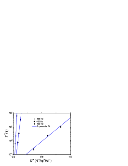
Figure 3: (Color online) Escape time as a function of $D^{-1}$ for $V_{g}=9.4~{}$V at different detunings $\omega-\omega_{b}$ from the bifurcation point.

In order to extract the scaling dependence of $E_{a}$ and $\Gamma_{0}$ on the detuning and the non-linear parameter $\gamma$ it is convenient to recall the predictions that can be obtained following Ref. Dykman and Krivoglaz (1979). Let us rescale the detuning by defining $\Omega=2|\omega-\omega_{0}|/\Delta\omega$ with $\Omega_{b}=2|\omega_{b}-\omega_{0}|/\Delta\omega$. For $\Omega_{b}\gg\sqrt{3}$ (that holds for all the data of our experiment) one obtains that $\Omega_{b}\approx 3|\gamma|f_{d}^{2}/(4\omega^{2}\Delta\omega^{2})$ with the parameters in Eq. (1) reading :

$$E_{a}=\frac{2f_{d}^{2}}{3\Delta\omega}{|\Omega-\Omega_{b}|^{3/2}\over\Omega_{b}^{5/2}},\,\Gamma_{0}=\frac{\Delta\omega}{2}\frac{|\Omega-\Omega_{b}|^{1/2}\Omega_{b}^{1/2}}{2\pi}.$$ (4)

The basic assumptions to obtain these expressions are that $E_{a}/D\gg 1$ in order to keep the escape a rare event, and to be able to reduce this two-dimensional problem (amplitude and phase) into a one-dimensional one. This second condition (much less appreciated in the literature) is only verified when the driving frequency $\omega$ is in a tiny region close to the bifurcation point $\omega_{b}$ and far from the frequency for which the amplitude is maximum. In this region, one of the eigenvalues of the linearized dynamical equations of motion vanishes, which induces a slow motion in the direction of the relative eigenvector. On the other hand when $\omega$ is such that the amplitude is maximal, the two eigenvalues coincide, inducing fully two-dimensional fluctuations. Thus beyond this point the approximation used to obtain Eq. (4) breaks down. This condition reads $4\Omega_{b}|\Omega-\Omega_{b}|\ll 1$.

(a)

(b)

Figure 4: (Color online) Scaling plots for $E_{a}$ (left) and $\Gamma_{0}$ (right) with respect to detuning. The full circles indicate the experimental points, the open (blue) triangles the prediction of the full numerical simulation, the (red) full lines the linear fit to the data, and the dashed (blue) lines the prediction of Eq. (4). Insets: scaling with the non-linear parameter $\Omega_{b}$.

In the experiment we performed this quantity ranged uniformly between 0.13 to 71, thus a part of the data where well outside the range of the expected validity of Eq. (4), enabling to investigate the behavior of $\Gamma$ in a region where no present analytical prediction exists. As explained, the expressions for $E_{a}$ and $\Gamma_{0}$ in Eq. (4) depend only on the detuning and the non linear coefficient (through $\Omega_{b}$), the other parameters being the same for all data points. To test the validity of Dykman-Krivoglaz expressions, we produce a scaling plot, where the logarithm of $E_{a}$ and $\Gamma_{0}$ are plotted as a function of $|\Omega-\Omega_{b}|/\Omega_{b}^{5/3}$ and $|\Omega-\Omega_{b}|\Omega_{b}$ (see Fig. 4). A remarkable scaling is then observed in all the experimental range, with a fitted slope as a function of the detuning of $1.53\pm 0.04$ and $0.55\pm 0.2$, for $E_{a}$ and $\Gamma_{0}$ respectively. This matches the analytic predictions by Dykman and Krivoglaz, and we use this good agreement to define the noise source calibration factor $C$: scaling $D$ by $C$ the prediction of Eq. (4) coincides with the fitted value for $E_{a}$ (dashed line in Fig. 4 left panel). The dependence on the non-linear parameter $\Omega_{b}$ could also be tested for both quantities. It is shown in the insets of Fig. 4 and gives fitted slopes of $-2.43\pm 0.05$ and $0.6\pm 0.1$, again in excellent agreement with Eq. (4).

To better understand this remarkable scaling in such a large parameter region we solved numerically the stochastic problem. This can be done by introducing the complex slow amplitude $z(t)$ defined as $x(t)=z(t)e^{i\omega t}+z(t)^{*}e^{-i\omega t}$ and then convert the Langevin Eq. (2) to a Fokker-Planck equation $\partial_{\tau}P={\cal L}P$ for the probability density $P(u,v,\tau)$ of the real and imaginary part of $z=(3|\gamma|/\Delta\omega)^{1/2}(u+iv)$ as a function of the dimensionless time $\tau=t\Delta\omega$. The escape rate from a given domain can be calculated by solving the equation ${\cal L}^{\dagger}\tau(u,v)=-1$ with zero boundary condition at the border of the domain Hänggi et al. (1990). This gives the average time needed to reach the border starting at $(u,v)$. The equation reads explicitly:

$$[{\cal D}(\partial^{2}_{u}+\partial^{2}_{v})-f_{u}\partial_{u}-f_{v}\partial_{v}]\tau=-1\,,$$ (5)

with ${\cal D}=3|\gamma|D/(8\omega^{3}\Delta\omega$), $f_{u}=u+v(u^{2}+v^{2})-\Omega$, $f_{v}=v-u(u^{2}+v^{2})-\Omega-F_{d}$, and $F_{d}=f_{d}(3|\gamma|)^{1/2}/[2(\omega\Delta\omega)^{3/2}$]. Eq. (5) can be solved numerically Pistolesi et al. (2008) to obtain the average escape time that coincides with the inverse of the sought Poissonian rate. The numerical results for $E_{a}$ and $\Gamma_{0}$ are shown in Fig. 4 in open (blue) triangles.

One can see that the exact (numerical) result has the same power law dependence as the analytical results (dashed line), even where the approximate theory is not supposed to hold. Quantitative agreement between experiment and theory on $E_{a}$ is obtained with $C\approx 1.3$, thus validating the experimental noise amplitude calibration to within 15 % which is remarkable. Note that the simulation does not contain any other free parameter, which are all experimentally known to better than 5 %. Concerning $\Gamma_{0}$, we are not aware of previous attempts to compare this quantity to the theoretical predictions. The agreement with the full theory is within a factor of about 3, which is remarkable given the logarithmic precision on this parameter. We speculate that these discrepancies could arise from the actual algorithm used to extract $\Gamma_{0}$, or from more fundamental reasons like extra (non-Duffing) nonlinearities appearing in Eq. (2) (i.e. non-linear damping, or non-cubic restoring force terms) .

In conclusion, we have investigated the escape dynamics close to the bifurcation point for a nanomechanical resonator in the Duffing non-linear regime measured at cryogenic temperatures. Using a single ideally tunable system, we have: (i) Measured the escape rate $\Gamma$ as a function of the noise amplitude $D$, the detuning to the bifurcation point $\omega-\omega_{b}$, and the nonlinear parameter $\gamma$. (ii) Extracted $E_{a}$ and $\Gamma_{0}$ as defined by Eq. (1). (iii) Verified that the universal scaling of $E_{a}$ and $\Gamma_{0}$ initially predicted for a tiny region around the bifurcation point holds actually in a region up to two orders of magnitude larger than the original one. (iv) Verified by solving numerically the exact problem, that the observation is in quantitative agreement with the behavior expected for a driven Duffing oscillator. The scaling of $E_{a}$ as a function of $|\Omega-\Omega_{b}|$ is consistent with the predictions of Refs. Dykman et al. (2005); Kogan (2008). Due to the generality of the Duffing model, these results are of interest for a wide class of systems. Even beyond the fundamental interest in the scaling laws we point out that the device acts as a very sensitive amplifier: it allows the detection of tiny variations of the resonator frequency. Understanding the frequency fluctuations in mechanical resonators is a current challenge of the field Fong et al. (2012); Zhang et al. (2014); van Leeuwen et al. (2014). Mastering of the bifurcation escape technique by having a reliable theory and experimental verification of the scaling of the rates is a crucial step towards the study of modifications induced by other phenomena.

We gratefully acknowledge discussions with M. Dykman, K. Hasselbach, E. Lhotel and A. Fefferman. We thank J. Minet and C. Guttin for help in setting up the experiment. We acknowledge support from MICROKELVIN, the EU FRP7 grant 228464 and of the French ANR grant QNM n^∘ 0404 01.

References

- Arrhenius (1889) S. Arrhenius, Z. Physik. Chem. 4, 226 (1889).
- Kramers (1940) H. A. Kramers, Physica 7, 284 (1940).
- Novak et al. (1995) M. A. Novak, R. Sessoli, A. Caneschi, and D. Gatteschi, J. of Magn. and Magn. Mater. 146, 211 (1995).
- Ozbudak et al. (2004) E. M. Ozbudak, M. Thattai, H. N. Lim, B. I. Shraiman, and A. van Oudenaarden, Nature 427, 737 (2004).
- Dethoff et al. (2012) E. A. Dethoff, J. Chugh, A. M. Mustoe, and H. M. Al-Hashimi, Nature 482, 322 (2012).
- Turlot et al. (1989) E. Turlot, D. Esteve, C. Urbina, J. M. Martinis, M. H. Devoret, S. Linkwitz, and H. Grabert, Phys. Rev. Lett. 62, 1788 (1989).
- Kurkijärvi (1972) J. Kurkijärvi, Phys. Rev. B 6, 832 (1972).
- Lapidus et al. (1999) L. J. Lapidus, D. Enzer, and G. Gabrielse, Phys. Rev. Lett. 83, 899 (1999).
- Siddiqi et al. (2004) I. Siddiqi, R. Vijay, F. Pierre, C. M. Wilson, M. Metcalfe, C. Rigetti, L. Frunzio, and M. H. Devoret, Phys. Rev. Lett. 93, 207002 (2004).
- Aldridge and Cleland (2005) J. S. Aldridge and A. N. Cleland, Phys. Rev. Lett. 94, 156403 (2005).
- Stambaugh and Chan (2006) C. Stambaugh and H. B. Chan, Phys. Rev. B 73, 172302 (2006).
- Chan and Stambaugh (2007) H. B. Chan and C. Stambaugh, Phys. Rev. Lett. 99, 060601 (2007).
- Chan et al. (2008) H. B. Chan, M. I. Dykman, and C. Stambaugh, Phys. Rev. Lett. 100, 130602 (2008).
- Unterreithmeier et al. (2010) Q. P. Unterreithmeier, T. Faust, and J. P. Kotthaus, Phys. Rev. B 81, 241405 (2010).
- Boulant et al. (2007) N. Boulant, G. Ithier, P. Meeson, F. Nguyen, D. Vion, D. Esteve, I. Siddiqi, R. Vijay, C. Rigetti, F. Pierre, and M. Devoret, Phys. Rev. B 76, 014525 (2007).
- Hänggi et al. (1990) P. Hänggi, P. Talkner, and M. Borkovec, Rev. Mod. Phys. 62, 251 (1990).
- Dykman and Krivoglaz (1979) M. I. Dykman and M. A. Krivoglaz, Sov. Phys. JETP , 60 (1979).
- Dykman et al. (2005) M. Dykman, I. Schwartz, and M. Shapiro, Phys. Rev. E 72, 021102 (2005).
- Kogan (2008) O. Kogan, arXiv:0805.0972v2 (2008).
- Collin et al. (2012) E. Collin, M. Defoort, K. Lulla, T. Moutonet, J.-S. Heron, O. Bourgeois, Y. M. Bunkov, and H. Godfrin, Review of Scientific Instruments 83, 045005 (2012).
- Cleland and Roukes (1999) A. Cleland and M. Roukes, Sensors and Actuators 72, 256 (1999).
- Collin et al. (2011a) E. Collin, T. Moutonet, J.-S. Heron, O. Bourgeois, Y. M. Bunkov, and H. Godfrin, J Low Temp Phys 162, 653 (2011a).
- Kozinsky et al. (2006) I. Kozinsky, H. W. C. Postma, I. Bargatin, and M. L. Roukes, Applied Physics Letters 88, 253101 (2006).
- Zaitsev et al. (2012) S. Zaitsev, O. Shtempluck, E. Buks, and O. Gottlieb, Nonlinear Dynamics 67, 859 (2012).
- Collin et al. (2011b) E. Collin, T. Moutonet, J.-S. Heron, O. Bourgeois, Y. M. Bunkov, and H. Godfrin, Phys. Rev. B 84, 054108 (2011b).
- Collin et al. (2010) E. Collin, Y. M. Bunkov, and H. Godfrin, Phys. Rev. B 82, 235416 (2010).
- Fong et al. (2012) K. Y. Fong, W. H. P. Pernice, and H. X. Tang, Phys. Rev. B 85, 161410(R) (2012).
- Zhang et al. (2014) Y. Zhang, J. Moser, J. Güttinger, A. Bachtold, and M. I. Dykman, Phys. Rev. Lett. 113, 255502 (2014).
- van Leeuwen et al. (2014) R. van Leeuwen, A. Castellanos-Gomez, G. Steele, H. van der Zant, and W. Venstra, Appl. Phys. Lett. 105, 041911 (2014).
- Eadie et al. (1971) W. Eadie, D. Drijard, F. James, M. Roos, and B. Sadoulet, Statistical Methods in Experimental Physics, edited by North-Holland (Amsterdam, 1971).
- Defoort (2014) M. Defoort, PhD thesis: Non-linear dynamics in nano-electromechanical systems at low temperature (CNRS et Université Grenoble Alpes, unpublished, 2014).
- Pistolesi et al. (2008) F. Pistolesi, Y. Blanter, and I. Martin, Physical Review B 78, 085127 (2008).