Tests of Lorentz and CPT Violation in the Medium Baseline Reactor Antineutrino Experiment

Abstract

Tests of Lorentz and CPT violation in the medium baseline reactor antineutrino experiment are presented in the framework of the Standard Model Extension (SME). Both the spectral distortion and sidereal variation are employed to derive the limits of Lorentz violation (LV) coefficients. We do the numerical analysis of the sensitivity of LV coefficients by taking the Jiangmen Underground Neutrino Observatory (JUNO) as an illustration, which can improve the sensitivity by more than two orders of magnitude compared with the current limits from reactor antineutrino experiments.

I Introduction

Special Relativity (SR) is a fundamental theory describing the Lorentz space-time symmetry, which is a consequence of the homogeneous and isotropic space-time and the principle of relativity among different inertial frames. Being a cornerstone of modern physics, SR has been verified with an extremely high degree of accuracy test . Although Lorentz invariance has been widely accepted, well-motivated models with Lorentz violation (LV) are anticipated from the principle of Quantum Gravity ssb . LV can be tested with the observations of high energy cosmic rays review , astrophysical neutrinos uhenu and gamma-ray bursts grb , as well as the low energy phenomena such as beta decays beta , double beta decays betabeta , atomic co-magnetometer experiments atomic and neutrino oscillations nulv .

The phenomena of neutrino oscillations have been well established from recent oscillation experiments with solar neutrinos, atmospheric neutrinos, reactor antineutrinos and accelerator neutrinos PDG . The standard picture of three active neutrino oscillations is described by three mixing angles, two independent mass-squared differences and the CP-violating phase. The next-generation neutrino oscillation experiments with higher precision are designed to probe the neutrino mass ordering and CP violation, and they also provide an opportunity to test new physics NP beyond the Standard Model (SM).

The low energy phenomena of LV can be systematically studied in the framework of the Standard Model Extension (SME) sme , which includes all possible LV terms formed by the SM fields in the Lagrangian,

$${\mathcal{L}}_{LV}\hskip 5.69046pt\simeq-(a_{L})_{\mu}\overline{\psi_{L}}\gamma^{\mu}\psi_{L}-(c_{L})_{\mu\nu}\overline{\psi_{L}}i\gamma^{\mu}\partial^{\nu}\psi_{L}.$$ (1)

Notice that $a_{L}$ violates both the Lorentz and CPT symmetries, but $c_{L}$ is CPT-even and only violates the Lorentz invariance. Although the LV coefficients are very small due to the suppression factor of the order of the electro-week scale divided by the Planck scale (i.e, $10^{-17}$), they provide an accessible test to Planck scale physics.

The SME framework predicts distinct behaviors for neutrino flavor conversions, which are very different from the standard picture of three active neutrino oscillations. The transition probability depends on the ratio of neutrino propagation distance $L$ and the neutrino energy $E$ (i.e., $L/E$) in the conventional oscillation theory, but in the SME it depends on either $L$ or $L\times E$ for the contribution induced by $a_{L}$ or $c_{L}$. On the other hand, LV also predicts the breakdown of space-time’s isotropy, which manifests as a sidereal modulation of the neutrino events for experiments with both the neutrino source and detector fixed on the earth. The sidereal time is defined on the basis of the earth’s orientation with respect to the sun-centered reference inertial frame, which will be defined in the next section. The sidereal variation of the experimental event rate will signify unambiguous evidence for LV. Previous LV searches in LSND lsnd , MINOS MINOS_near ; MINOS_far , MiniBooNE MiniBooNE and Double Chooz chooz are reported with the limit level ranging from $10^{-20}$ to $10^{-23}$, where $a_{L}$ is in the unit of GeV and $c_{L}$ is unitless.

In the present work we will study the possible tests of Lorentz and CPT violation in the medium baseline reactor antineutrino experiment. We reformulate the theoretical description of vacuum neutrino oscillations in the SME framework, and discuss the key factors that affect the sensitivity of LV. Using both the spectral distortion and sidereal variation effects, we present the sensitivity of LV coefficients for the medium baseline reactor antineutrino experiment taking the Jiangmen Underground Neutrino Observatory (JUNO) as an illustration. Our analyses are carried out in the reference frame of the sun, which is defined in Ref. frame , and has been used in the neutrino oscillation experiments lsnd ; MINOS_near ; MINOS_far ; MiniBooNE ; chooz .

The remaining part of this work is organized as follows. Section 2 is to derive the theoretical description. We present the neutrino oscillation probability in the SME framework, and define the standard and local frames to denote the direction-dependent property of LV. In section 3, we give the numerical analysis for JUNO and calculate its sensitivity to the relevant LV coefficients. Finally, we conclude in section 4.

II Theoretical Description

According to the SME, the effective Hamiltonian for Lorentz violating neutrino oscillations is written as lv

$$H_{\alpha\beta}=\displaystyle\frac{1}{E}\hskip 1.42271pt\left[\hskip 1.42271pt\displaystyle\frac{m^{2}}{2}+(a_{L})_{\mu}p^{\mu}+(c_{L})_{\mu\nu}p^{\mu}p^{\nu}\hskip 1.42271pt\right]_{\alpha\beta},$$ (2)

where $E$ and $p^{\mu}$ are the neutrino energy and 4-momentum, $\alpha$ and $\beta$ are flavor indices, and $(m^{2})_{\alpha\beta}=U{\rm diag}(m^{2}_{1},m^{2}_{2},m^{2}_{3})U^{\rm\dagger}$ is the mass-squared matrix in the flavor basis with $U$ being the Pontecorvo-Maki-Nakagawa-Sakata (PMNS) matrix PMNS . $a_{L}$ and $c_{L}$ are the LV coefficients defined in Eq. (1), and from dimensional analyses one can observe that $a_{L}$ is dimension-one while $c_{L}$ is dimensionless. Taking account of the CPT transformation property of $H$ cpt , we find that the Hamiltonian for antineutrinos has the following form

$$H_{\alpha\beta}=\displaystyle\frac{1}{E}\hskip 1.42271pt\left[\hskip 1.42271pt\displaystyle\frac{m^{2}}{2}-(a_{L})_{\mu}p^{\mu}+(c_{L})_{\mu\nu}p^{\mu}p^{\nu}\hskip 1.42271pt\right]_{\alpha\beta}^{*}\,.$$ (3)

To derive the antineutrino oscillation probabilities from the above Hamiltonian, we employ the perturbative treatment as in Ref. long to factorize the LV part from the conventional neutrino oscillation part. This approximate treatment is reasonable for the situation with significant oscillation effects (i.e., long baseline).

In the standard framework of three active antineutrino oscillations, the oscillation probability can be expressed as the square of a time evolution operator $S^{(0)}$:

$$P^{(0)}_{\alpha\rightarrow\beta}=\left|S^{(0)}_{\alpha\beta}\right|^{2}=\left|(e^{-iH_{0}t})_{\alpha\beta}\right|^{2}=\left|\sum_{i}\hskip 1.42271ptU_{\alpha i}\hskip 1.42271ptU_{\beta i}^{*}\hskip 1.42271pte^{-iE_{i}t}\right|^{2},$$ (4)

where $H_{0}=(m^{2})^{*}/(2E)$ is the mass term of the Hamiltonian in Eq. (3), and $t\simeq L$ for ultra-relativistic particles. By defining $\delta H=[-(a_{L})_{\mu}p^{\mu}+(c_{L})_{\mu\nu}p^{\mu}p^{\nu}]^{*}/E$ and taking the perturbative expansion, we derive the whole time evolution operator as

$$\begin{array}[]{ll}\vspace{0.2cm}S&=\hskip 5.69046pte^{-iHt}\hskip 5.69046pt=\hskip 5.69046pt\left(e^{-iH_{0}t-i\delta Ht}\hskip 1.42271pte^{iH_{0}t}\right)\hskip 1.42271pte^{-iH_{0}t}\\ \vspace{0.2cm}&=\hskip 5.69046pt\left(1-i\int_{0}^{t}dt_{1}\hskip 1.42271pte^{-iH_{0}t_{1}}\hskip 1.42271pt\delta H\hskip 1.42271pte^{iH_{0}t_{1}}+\cdots\right)S^{(0)}\\ &=\hskip 5.69046ptS^{(0)}+S^{(1)}+\cdots,\end{array}$$ (5)

where the higher order contributions are omitted. Consequently, the oscillation probability is expanded as

$$P_{\alpha\rightarrow\beta}\hskip 2.84544pt=\hskip 2.84544pt\left|S_{\alpha\beta}\right|^{2}\hskip 2.84544pt=\hskip 2.84544pt\left|\hskip 1.42271ptS^{(0)}_{\alpha\beta}\hskip 1.42271pt\right|^{2}+2\hskip 1.42271pt{\rm Re}\hskip 1.42271pt\left[\hskip 1.42271pt(S^{(0)}_{\alpha\beta})^{*}\hskip 1.42271ptS^{(1)}_{\alpha\beta}\hskip 1.42271pt\right]\hskip 2.84544pt=\hskip 2.84544ptP^{(0)}_{\alpha\rightarrow\beta}+P^{(1)}_{\alpha\rightarrow\beta}.$$ (6)

In particular, the explicit form of $P^{(1)}_{\alpha\rightarrow\beta}$ can be written as long

$$P^{(1)}_{\alpha\rightarrow\beta}=\displaystyle{\sum_{i,j}}\hskip 1.42271pt{\displaystyle\sum_{\rho,\sigma}}\hskip 1.42271pt2\hskip 1.42271ptL\hskip 1.42271pt{\rm Im}\hskip 1.42271pt\left[\hskip 1.42271pt(S^{(0)}_{\alpha\beta})^{*}\hskip 1.42271ptU_{\alpha i}\hskip 1.42271ptU_{\rho i}^{*}\hskip 1.42271pt\tau_{ij}\hskip 1.42271pt\delta H_{\rho\sigma}\hskip 1.42271ptU_{\sigma j}\hskip 1.42271ptU_{\beta j}^{*}\hskip 1.42271pt\right],$$ (7)

with

$$\tau_{ij}=\left\{\begin{array}[]{cc}\vspace{0.2cm}\exp{\{-iE_{i}L\}}&\hskip 8.5359pt{\rm when}\hskip 8.5359pti=j\\ \displaystyle\frac{\exp{\{-iE_{i}L\}}-\exp{\{-iE_{j}L\}}}{-i(E_{i}-E_{j})L}&\hskip 8.5359pt{\rm when}\hskip 8.5359pti\neq j\end{array}\right..$$ (8)

The hermiticity of Hamiltonian requires $\delta H_{\rho\sigma}$ to be real when $\rho=\sigma$ and $\delta H_{\rho\sigma}=\delta H_{\sigma\rho}^{*}$ when $\rho\neq\sigma$. For the former case, the LV terms can be extracted directly as

$$P^{(1)}_{\alpha\rightarrow\beta}=\displaystyle{\sum_{i,j}}\hskip 1.42271pt{\displaystyle\sum_{\rho=\sigma}}\hskip 1.42271pt2\hskip 1.42271ptL\hskip 1.42271pt{\rm Im}\hskip 1.42271pt\left[(S^{(0)}_{\alpha\beta})^{*}\hskip 1.42271ptU_{\alpha i}\hskip 1.42271ptU_{\rho i}^{*}\hskip 1.42271pt\tau_{ij}\hskip 1.42271pt\hskip 1.42271ptU_{\sigma j}\hskip 1.42271ptU_{\beta j}^{*}\right]\delta H_{\rho\sigma}.$$ (9)

As for the latter one, if we neglect the CP phase of the PMNS matrix in the following analysis, the LV terms can be expressed as

$$\begin{array}[]{ll}\vspace{0.2cm}P^{(1)}_{\alpha\rightarrow\beta}&={\displaystyle\sum_{i,j}}\hskip 1.42271pt\displaystyle{\sum_{\rho\neq\sigma}}\hskip 1.42271ptL\hskip 1.42271pt{\rm Im}\hskip 1.42271pt\left[(S^{(0)}_{\alpha\beta})^{*}\hskip 1.42271ptU_{\alpha i}\hskip 1.42271ptU_{\rho i}\hskip 1.42271pt\tau_{ij}\hskip 1.42271ptU_{\sigma j}\hskip 1.42271ptU_{\beta j}(\delta H_{\rho\sigma}+\delta H_{\sigma\rho})\right]\\ &={\displaystyle\sum_{i,j}}\hskip 1.42271pt\displaystyle{\sum_{\rho\neq\sigma}}\hskip 1.42271pt2\hskip 1.42271ptL\hskip 1.42271pt{\rm Im}\hskip 1.42271pt\left[(S^{(0)}_{\alpha\beta})^{*}\hskip 1.42271ptU_{\alpha i}\hskip 1.42271ptU_{\rho i}\hskip 1.42271pt\tau_{ij}\hskip 1.42271pt\hskip 1.42271ptU_{\sigma j}\hskip 1.42271ptU_{\beta j}\right]\hskip 1.42271pt{\rm Re}\hskip 1.42271pt\delta H_{\rho\sigma}.\end{array}$$ (10)

From the expressions in Eqs. (9) and (10), we notice that contributions from the mass term and LV terms can be factorized. Therefore, we define the quantity $I_{\alpha\beta}^{\rho\sigma}$ as an indicator of the sensitivity to $\delta H_{\rho\sigma}$ in a certain oscillation channel $P_{\alpha\to\beta}$,

$$I_{\alpha\beta}^{\rho\sigma}={\displaystyle\sum_{i,j}}\hskip 1.42271pt2\hskip 1.42271ptL\hskip 1.42271pt{\rm Im}\hskip 1.42271pt\left[(S^{(0)}_{\alpha\beta})^{*}\hskip 1.42271ptU_{\alpha i}\hskip 1.42271ptU_{\rho i}\hskip 1.42271pt\tau_{ij}\hskip 1.42271ptU_{\sigma j}\hskip 1.42271ptU_{\beta j}\right].$$ (11)

This indicator can be used to understand the distinct properties of different LV components $\delta H_{\rho\sigma}$ in the following numerical analysis.

Figure 1: The definition of the sun-centered system frame .

Figure 2: The definition of $t=0$ in the sun-centered system.

In the above expressions of the oscillation probability, the most important property of the LV coefficients is that $(a_{L})_{\mu}$ and $(c_{L})_{\mu\nu}$ are direction-dependent. Thus a reference frame should be specified when an experiment is going to report its LV results. The sun can take on this responsibility, because it can be taken as an inertial frame to a good approximation frame . In the reference frame of the sun, the choice of the sun-centered system lsnd is depicted in Fig. 2 and defined in the following way:

• Point $S$ is the center of the sun;

• The $Z$ axis has the same direction as the earth’s rotational axis, so the $X$-$Y$ plane is parallel to the earth’s equator;

• The $X$ axis is parallel to the vector pointed from the sun to the autumnal equinox, while the $Y$ axis completes the right-handed system.

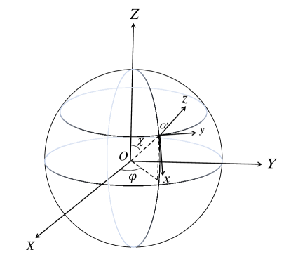
Figure 3: The definition of the earth-centered system frame .

Figure 4: The definition of the local coordinate system.

In a terrestrial experiment, the direction of neutrino propagation is described by its components along the $X,Y,Z$ axes (i.e., $\hat{N}^{X},\hat{N}^{Y}$ and $\hat{N}^{Z}$). For convenience, the origin of the sun-centered system can be defined to be located in the center of the earth $O$ due to the invariance of spatial translation, which is defined in Fig. 4. In order to express $\hat{N}^{X},\hat{N}^{Y}$ and $\hat{N}^{Z}$ in terms of local geographical information, a local coordinate system $(x,y,z)$ is also introduced:

• point $O^{\prime}$ is the site of the neutrino source, and $\chi$ (i.e., the angle between $OO^{\prime}$ and $Z$ axis) denotes its colatitude;

• the $z$ axis is defined to be upward;

• the $x$ and $y$ axes point to the south and east, respectively.

In the local coordinate system depicted in Fig. 4, the direction of neutrino propagation is parameterized by two angles, where $\theta$ is the angle between the beam direction and $z$ axis and $\phi$ is the angle between the beam direction and $x$ axis.

Because the neutrino source and detector are fixed on the earth, the rotation of the earth will induce a periodic change of the neutrino propagating directions relative to the standard reference frame, with an angular frequency $\omega=2\pi/T_{\rm s}$. Here $T_{\rm s}\simeq 23\hskip 2.84544pt{\rm h}\hskip 2.84544pt56\hskip 2.84544pt{\rm min}$ is the period of a sidereal day. For this reason, a reference time origin should be specified. Without loss of generality, we can set the local midnight when the earth arrives at the autumnal equinox to be $t=0$ (see Fig. 2). At this moment, the $x$-$z$ plane coincidences with the $X$-$Z$ plane, resulting in the coordinate transformation as

$$\begin{array}[]{lll}\hat{N}^{X}&=&\cos{\chi}\sin{\theta}\cos{\phi}+\sin{\chi}\cos{\theta},\\ \hat{N}^{Y}&=&\sin{\theta}\sin{\phi},\\ \hat{N}^{Z}&=&-\sin{\chi}\sin{\theta}\cos{\phi}+\cos{\chi}\cos{\theta}.\end{array}$$ (12)

Therefore, the direction of neutrino propagation $\widehat{p^{\mu}}=(1,\ \widehat{p^{X}},\ \widehat{p^{Y}},\ \widehat{p^{Z}})$ is a periodic function of the time $t$

$$\begin{array}[]{lll}\widehat{p^{X}}&=&\hat{N}^{X}\cos{\omega t}-\hat{N}^{Y}\sin{\omega t},\\ \widehat{p^{Y}}&=&\hat{N}^{X}\cos{\omega t}+\hat{N}^{Y}\sin{\omega t},\\ \widehat{p^{Z}}&=&\hat{N}^{Z}.\end{array}$$ (13)

Accordingly, $\delta H_{\rho\sigma}$ can be decomposed as

$$\begin{array}[]{ll}\delta H_{{\rho\sigma}}=&\mathcal{C}_{{\rho\sigma}}+(\mathcal{A}_{s})_{\rho\sigma}\sin{\omega t}+(\mathcal{A}_{c})_{\rho\sigma}\cos{\omega t}\\ &+(\mathcal{B}_{s})_{\rho\sigma}\sin{2\omega t}+(\mathcal{B}_{c})_{\rho\sigma}\cos{2\omega t}.\end{array}$$ (14)

Note that the above coefficients (i.e., $\mathcal{C}$, $\mathcal{A}_{s}$, $\mathcal{A}_{c}$, $\mathcal{B}_{s}$ and $\mathcal{B}_{c}$) are linear combinations of the LV coefficients $(a_{L})_{\mu}$ and $(c_{L})_{\mu\nu}$. Among them, terms of $\mathcal{A}_{s}$, $\mathcal{A}_{c}$, $\mathcal{B}_{s}$ and $\mathcal{B}_{c}$ (written as $\mathcal{A/B}$ for short) are time-dependent and can induce periodic variations for the oscillation probability. On the other hand, $\mathcal{C}$ term can modify the absolute value of the oscillation probability with unconventional energy and baseline dependence, while the contributions of $\mathcal{A/B}$ cancel out in a full sidereal period.

III Numerical analysis

In this section, we discuss two distinct LV effects in the medium baseline reactor antineutrino experiment. The first one is the spectral distortion in the reactor antineutrino oscillation probability $P_{ee}$, and the second one is the sidereal modulation of the antineutrino event rate. Previous experimental LV searches mainly focus on the signature of sidereal modulation as it can give definite evidence for LV and is independent of the uncertainties of oscillation probabilities. However, as all the three mixing angles and two mass-squared differences are measured with high precision, it is desirable to place compatible constraints on LV coefficients using the spectral distortion information. Therefore, we employ both the phenomena to constrain LV coefficients.

In our numerical analysis, we take the JUNO experiment DYB2 ; JUNO as a working example. We simplify the reactor complexes in Yangjiang (labeled with “1”) and Taishan (labeled with “2”) as two virtual reactors with equal baselines (i.e., 53 km). Meanwhile, a 20 kton liquid scintillator detector is located in Jiangmen. The antineutrinos coming from the two reactors can be written as

$$\phi_{1}(E)=N_{1}\hskip 1.42271ptp_{1}(E)\ ,\hskip 28.45274pt\phi_{2}(E)=N_{2}\hskip 1.42271ptp_{2}(E)\ ,$$ (15)

where $N_{1}$ and $N_{2}$ are the total antineutrino events during the experimental period, while $p_{1}(E)$ and $p_{2}(E)$ are their spectrum distributions. For simplicity, we assume $p_{1}(E)=p_{2}(E)=p(E)$ and take the fuel composition as $53.8\%$ ${}^{235}{\rm U}$, $7.8\%$ ${}^{238}{\rm U}$, $32.8\%$ ${}^{239}{\rm Pu}$ and $5.6\%$ ${}^{239}{\rm Pu}$. The reactor antineutrino spectra are described by the following phenomenological expressions distribution ,

$$\begin{array}[]{lll}\vspace{0.3cm}p_{235}(E)&=&\displaystyle\frac{1}{1.96}\hskip 1.42271pt\exp\hskip 1.42271pt[\hskip 1.42271pt3.2-3.1E+1.4E^{2}-0.37E^{3}+0.045E^{4}-0.0021E^{5}\hskip 1.42271pt]\ ,\\ \vspace{0.3cm}p_{238}(E)&=&\displaystyle\frac{1}{2.53}\hskip 1.42271pt\exp\hskip 1.42271pt[\hskip 1.42271pt0.48+0.19E-0.13E^{2}-0.0068E^{3}+0.0022E^{4}-0.00015E^{5}\hskip 1.42271pt]\ ,\\ \vspace{0.3cm}p_{239}(E)&=&\displaystyle\frac{1}{1.52}\hskip 1.42271pt\exp\hskip 1.42271pt[\hskip 1.42271pt6.4-7.4E+3.5E^{2}-0.88E^{3}+0.10E^{4}-0.0046E^{5}\hskip 1.42271pt]\ ,\\ p_{241}(E)&=&\displaystyle\frac{1}{1.88}\hskip 1.42271pt\exp\hskip 1.42271pt[\hskip 1.42271pt3.3-3.2E+1.4E^{2}-0.37E^{3}+0.043E^{4}-0.0019E^{5}\hskip 1.42271pt]\ .\end{array}$$ (16)

As a consequence, $p(E)$ is a weighted average as

$$p(E)=0.538\hskip 1.42271ptp_{235}(E)+0.078\hskip 1.42271ptp_{238}(E)+0.328\hskip 1.42271ptp_{239}(E)+0.056\hskip 1.42271ptp_{241}(E)\ .$$ (17)

Finally, the event number distribution can be obtained as a function of $E_{\rm o}$,

$$n^{(0)}(E_{\rm o})=\int_{E_{\rm th}}^{\infty}\mathcal{N}\hskip 1.42271pt[N_{1}+N_{2}]\hskip 1.42271ptp(E)\hskip 1.42271ptP_{ee}^{(0)}\hskip 1.42271pt\sigma(E)\hskip 1.42271ptG(E_{\rm o},E)\hskip 1.42271ptdE\ .$$ (18)

Here $E_{\rm o}\simeq E_{e}+1.3\,({\rm MeV})$, with $E_{e}$ being the energy of the outgoing positron in the inverse beta decay (IBD) process. $G(E_{\rm o},E)$ is a Gaussian distribution for the energy resolution, with the standard deviation defined as

$$\rho\simeq 0.03\sqrt{E_{\rm o}-0.8}\ .$$ (19)

$\mathcal{N}$ is a normalization factor including the effects of reactor power, detection efficiency and the detector size. With the approximation of equal baselines, the survival probability for $\bar{\nu}_{e}$ from the two different sources can be taken as the same one

$$P_{ee}^{(0)}=1-4s_{12}^{2}c_{12}^{2}c_{13}^{4}\sin^{2}{\frac{\Delta m_{21}^{2}L}{4E}}-4s_{13}^{2}c_{13}^{2}c_{12}^{2}\sin^{2}{\frac{\Delta m_{31}^{2}L}{4E}}-4s_{13}^{2}c_{13}^{2}s_{12}^{2}\sin^{2}{\frac{\Delta m_{32}^{2}L}{4E}}\ ,$$ (20)

where $s_{ij}=\sin\theta_{ij}$, $c_{ij}=\cos\theta_{ij}$ and $\Delta m_{ij}^{2}=m^{2}_{i}-m^{2}_{j}$ are the neutrino mixing angles defined in the standard parameterization PDG and mass squared differences, respectively. $\sigma(E)$ is the leading-order IBD cross section cross

$$\sigma(E)\simeq 0.0952(E-1.3)\sqrt{(E-1.3)^{2}-0.5^{2}}\times 10^{-42}\ {\rm cm}^{2}.$$ (21)

As discussed in Ref. JUNO , about one hundred thousand IBD events are expected after a nominal running of six years. Therefore, we normalize the total events in Eq. (18) to be one hundred thousand.

When LV effects are included, the energy distribution of the IBD events receives an extra contribution,

$$n^{(1)}(E_{\rm o})=\int_{E_{\rm th}}^{\infty}\mathcal{N}\hskip 1.42271ptp(E)\hskip 1.42271pt\left[\hskip 1.42271ptN_{1}\hskip 1.42271pt(P_{ee}^{(1)})_{1}+N_{2}\hskip 1.42271pt(P_{ee}^{(1)})_{2}\hskip 1.42271pt\right]\hskip 1.42271pt\sigma(E)\hskip 1.42271ptG(E_{\rm o},E)\hskip 1.42271ptdE\ .$$ (22)

For simplicity, we define an effective LV-induced oscillation probability as

$$\begin{array}[]{ll}\vspace{0.3cm}P_{ee}^{(1){\rm eff}}&=\displaystyle\frac{1}{N_{1}+N_{2}}\hskip 1.42271pt\left[\hskip 1.42271ptN_{1}\hskip 1.42271pt(P_{ee}^{(1)})_{1}+N_{2}\hskip 1.42271pt(P_{ee}^{(1)})_{2}\hskip 1.42271pt\right]\\ &={\displaystyle\sum_{i,j}}\hskip 1.42271pt{\displaystyle\sum_{\rho,\sigma}}\hskip 1.42271pt2\hskip 1.42271ptL\hskip 1.42271pt{\rm Im}\hskip 1.42271pt\left[\hskip 1.42271pt(S^{(0)}_{ee})^{*}\hskip 1.42271ptU_{ei}\hskip 1.42271ptU_{\rho i}^{*}\hskip 1.42271pt\tau_{ij}\hskip 1.42271pt\delta H_{\rho\sigma}^{\rm eff}\hskip 1.42271ptU_{\sigma j}\hskip 1.42271ptU_{ej}^{*}\hskip 1.42271pt\right]\ ,\end{array}$$ (23)

where

$$\delta H_{\rho\sigma}^{\rm eff}=\displaystyle\frac{1}{N_{1}+N_{2}}\hskip 1.42271pt\left[\hskip 1.42271ptN_{1}\hskip 1.42271pt(\delta H_{\rho\sigma})_{1}+N_{2}\hskip 1.42271pt(\delta H_{\rho\sigma})_{2}\hskip 1.42271pt\right]\ .$$ (24)

Antineutrinos from two reactor sources have different propagation directions, so $(\delta H_{\rho\sigma})_{1}$ and $(\delta H_{\rho\sigma})_{2}$ can be expanded in the same way as Eq. (14), with the information of the detector and reactor position pos . For LV coefficients $a_{L}^{\mu}$ and $c_{L}^{\mu\nu}$ with arbitrary directions, the expansion coefficients for antineutrinos coming from Yangjiang are given as

$$\begin{array}[]{lll}\vspace{0.2cm}(\mathcal{C}_{\rho\sigma}^{*})_{1}&=&-a^{T}_{\rho\sigma}+0.81\ a^{Z}_{\rho\sigma}+[\ 0.42\ c^{TT}_{\rho\sigma}-0.48\ c^{ZZ}_{\rho\sigma}\ ]\ E,\\ \vspace{0.2cm}((\mathcal{A}_{s})_{\rho\sigma}^{*})_{1}&=&-0.49\ a^{X}_{\rho\sigma}-0.33\ a^{Y}_{\rho\sigma}-[\ 0.98\ c^{TX}_{\rho\sigma}+0.65\ c^{TY}_{\rho\sigma}-0.79\ c^{XZ}_{\rho\sigma}-0.52\ c^{YZ}_{\rho\sigma}\ ]\ E,\\ \vspace{0.2cm}((\mathcal{A}_{c})_{\rho\sigma}^{*})_{1}&=&-0.33\ a^{X}_{\rho\sigma}+0.49\ a^{Y}_{\rho\sigma}-[\ 0.65\ c^{TX}_{\rho\sigma}-0.98\ c^{TY}_{\rho\sigma}-0.52\ c^{XZ}_{\rho\sigma}+0.79\ c^{YZ}_{\rho\sigma}\ ]\ E,\\ \vspace{0.2cm}((\mathcal{B}_{s})_{\rho\sigma}^{*})_{1}&=&-0.16\ c_{\rho\sigma}^{XX}+0.16\ c_{\rho\sigma}^{YY}+0.13\ c_{\rho\sigma}^{XY},\\ \vspace{0.2cm}((\mathcal{B}_{c})_{\rho\sigma}^{*})_{1}&=&-0.067\ c_{\rho\sigma}^{XX}+0.067\ c_{\rho\sigma}^{YY}+0.32\ c_{\rho\sigma}^{XY}.\end{array}$$ (25)

while the expansion coefficients for antineutrinos coming from Taishan are given as

$$\begin{array}[]{lll}\vspace{0.2cm}(\mathcal{C}_{\rho\sigma}^{*})_{2}&=&-a^{T}_{\rho\sigma}+0.41\ a^{Z}_{\rho\sigma}-[\ 0.59\ c^{TT}_{\rho\sigma}-0.25\ c^{ZZ}_{\rho\sigma}\ ]\ E,\\ \vspace{0.2cm}((\mathcal{A}_{s})_{\rho\sigma}^{*})_{2}&=&0.90\ a^{X}_{\rho\sigma}-0.17\ a^{Y}_{\rho\sigma}+[\ 1.8\ c^{TX}_{\rho\sigma}-0.34\ c^{TY}_{\rho\sigma}-0.73\ c^{XZ}_{\rho\sigma}+0.14\ c^{YZ}_{\rho\sigma}\ ]\ E,\\ \vspace{0.2cm}((\mathcal{A}_{c})_{\rho\sigma}^{*})_{2}&=&-0.17\ a^{X}_{\rho\sigma}-0.90\ a^{Y}_{\rho\sigma}-[\ 0.34\ c^{TX}_{\rho\sigma}+1.8\ c^{TY}_{\rho\sigma}-0.14\ c^{XZ}_{\rho\sigma}-0.73\ c^{YZ}_{\rho\sigma}\ ]\ E,\\ \vspace{0.2cm}((\mathcal{B}_{s})_{\rho\sigma}^{*})_{2}&=&0.15\ c_{\rho\sigma}^{XX}-0.15\ c_{\rho\sigma}^{YY}+0.77\ c_{\rho\sigma}^{XY},\\ \vspace{0.2cm}((\mathcal{B}_{c})_{\rho\sigma}^{*})_{2}&=&-0.39\ c_{\rho\sigma}^{XX}+0.39\ c_{\rho\sigma}^{YY}-0.30\ c_{\rho\sigma}^{XY}.\end{array}$$ (26)

Here the subscript “_L” for $a_{L}$ and $c_{L}$ is omitted for simplicity.

The energy range from 1.8 to 8 $\hskip 2.84544pt{\rm MeV}$ is divided into 200 equal-size bins. For each bin with the label $i$, the expected event number can be calculated as

$$n_{i}^{(0)}=\int_{E_{i}-\Delta E}^{E_{i}+\Delta E}n^{(0)}(E_{\rm o})\hskip 2.84544ptdE_{\rm o}\ ,$$ (27)

where $\Delta E\simeq 0.031\hskip 2.84544pt{\rm MeV}$ and $E_{i}=[\hskip 1.42271pt1.8+(i-0.5)\hskip 1.42271pt\Delta E\hskip 1.42271pt]\hskip 2.84544pt{\rm MeV}$. In this calculation, the oscillation parameters are taken as the central values of the recent global-fit analysis fit ,

$$\begin{array}[]{ll}\sin^{2}{\theta_{12}}=0.323\ ,&\hskip 28.45274pt\sin^{2}{\theta_{13}}=0.0234\ ;\\ \Delta m_{21}^{2}=7.60\times 10^{-5}\ \rm{eV^{2}}\ ,&\hskip 28.45274pt\Delta m_{31}^{2}=2.48\times 10^{-3}\ \rm{eV^{2}}\ .\end{array}$$ (28)

Furthermore, the event numbers from the LV terms are calculated as

$$n_{i}^{(1)}=\int_{E_{i}-\Delta E}^{E_{i}+\Delta E}n^{(1)}(E_{\rm o})\hskip 2.84544ptdE_{\rm o}\ .$$ (29)

Because $\delta H_{\rho\sigma}^{\rm eff}$ has an identical form as Eq. (14), we can define the effective coefficients $\mathcal{C}_{\rho\sigma}^{\rm eff}$ and $\mathcal{A/B}_{\rho\sigma}^{\rm eff}$ as the weighted averages of $(\mathcal{C}_{\rho\sigma})_{1/2}$ and $(\mathcal{A/B}_{\rho\sigma})_{1/2}$.

$\mathcal{C}_{\rho\sigma}^{\rm eff}$ can modify the energy dependence of the oscillation probability.

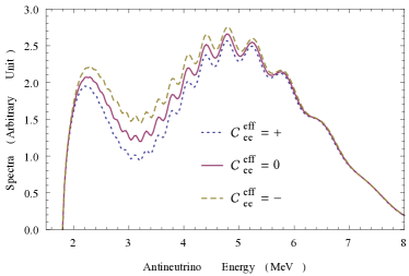
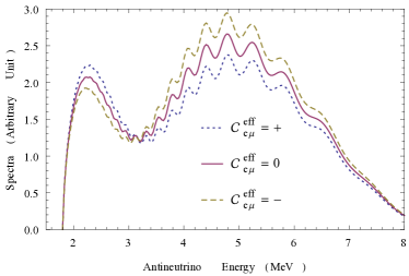
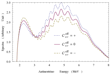
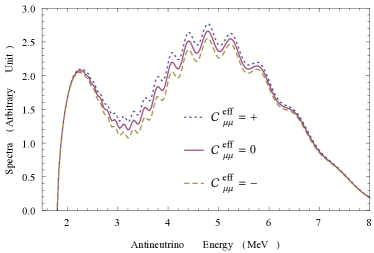
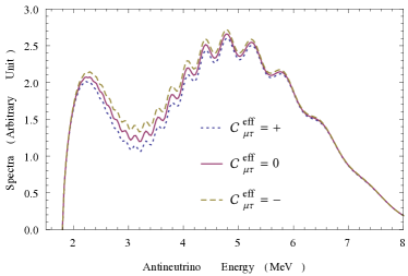
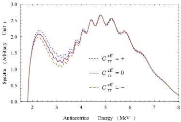
Figure 5: Spectral distortion effects for the six effective LV coefficients. Their magnitudes are taken as $(\pm 5.0\times 10^{-22})\,{\rm GeV}$ and zero for comparison.

Fig. (5) shows the spectral distortion effects for the six effective LV coefficients $\mathcal{C}_{\rho\sigma}^{\rm eff}$. Their magnitudes are taken as $(\pm 5.0\times 10^{-22})\,{\rm GeV}$ for comparison. The standard case without LV is also illustrated. Therefore, we can constrain the magnitude of $\mathcal{C}_{\rho\sigma}^{\rm eff}$ by comparing the observed spectrum with the expected one. There are many $\mathcal{C}_{\rho\sigma}^{\rm eff}$ components and they may be cancelled with each other when combined together. For definiteness, we shall take only one non-zero coefficient at one time in the analysis.

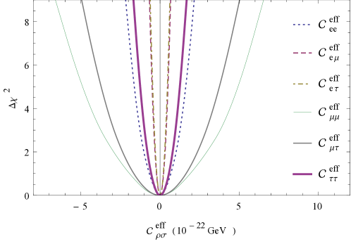
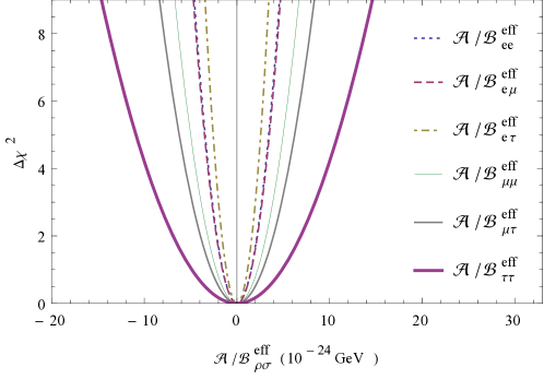
Figure 6: The JUNO sensitivity for the effective LV coefficients from the spectral distortion (upper panel) and sidereal variation (lower panel) effects.

To quantify the significance of LV effects in the spectral distortion, a $\chi^{2}$ function is defined as follows:

$$\chi^{2}=\sum_{i}\frac{\left[n_{i}^{(0)}(s^{2}_{12})-\left(n_{i}^{(0)\prime}(s_{12}^{\prime 2})+n_{i}^{(1)}\right)(1+\epsilon)\right]^{2}}{n_{i}^{(0)}(s^{2}_{12})+\left(0.01n_{i}^{(0)}(s^{2}_{12})\right)^{2}}+\frac{\epsilon^{2}}{0.05^{2}}+\frac{(s_{12}^{\prime 2}-s_{12}^{2})^{2}}{0.016^{2}}\,,$$ (30)

where two pull-parameters are included. $\epsilon$ is a normalization factor with an uncertainty of 0.05, $s_{12}^{\prime 2}$ is the oscillation parameter that affects the analysis most. The uncertainty of $s_{12}^{2}$ is also taken from Ref. fit . We also take a spectral uncertainty of the $1\%$ level, which is assumed uncorrelated among different energy bins. For each $\mathcal{C}_{\rho\sigma}^{\rm eff}$, we can obtain a one-dimensional $\Delta\chi^{2}$ function after marginalizing the pull-parameters $\epsilon$ and $s_{12}^{\prime 2}$. The distributions of $\Delta\chi^{2}$ as functions of the six effective LV coefficients $\mathcal{C}_{\rho\sigma}^{\rm eff}$ are shown in the upper panel of Fig. (6). The upper limits at the $95\%$ confidence level for these LV coefficients are listed in the first row of Table 1. The relative differences in the power of constraining these six coefficients can be understood by the quantity defined in Eq. (11), which indicates that the flavor indices with larger $I_{\alpha\beta}$ will get more severe constraints.

	$\mathcal{C}_{ee}^{{\rm eff}}$	$\hskip 2.84544pt\mathcal{C}_{e\mu}^{{\rm eff}}$	$\hskip 2.84544pt\mathcal{C}_{e\tau}^{{\rm eff}}$	$\mathcal{C}_{\mu\mu}^{{\rm eff}}$	$\hskip 2.84544pt\mathcal{C}_{\mu\tau}^{{\rm eff}}$	$\mathcal{C}_{\tau\tau}^{{\rm eff}}$
$10^{-22}\ {\rm GeV}$	1.5	0.5	0.4	4.4	3.4	1.1
	$\mathcal{A/B}_{ee}^{{\rm eff}}$	$\hskip 2.84544pt\mathcal{A/B}_{e\mu}^{{\rm eff}}$	$\hskip 2.84544pt\mathcal{A/B}_{e\tau}^{{\rm eff}}$	$\mathcal{A/B}_{\mu\mu}^{{\rm eff}}$	$\hskip 2.84544pt\mathcal{A/B}_{\mu\tau}^{{\rm eff}}$	$\mathcal{A/B}_{\tau\tau}^{{\rm eff}}$
$10^{-24}\ {\rm GeV}$	3.7	3.7	2.7	5.4	6.6	11.6

Table 1: The JUNO sensitivity at the $95\%$ confidence level for the effective LV coefficients $\mathcal{C}$, $\mathcal{A/B}$ in $\delta H_{\rho\sigma}^{{\rm eff}}$.

Next we shall discuss the constraints on the effective coefficients $\mathcal{A/B}_{\rho\sigma}^{\rm eff}$ from the sidereal variation of IBD event rates. For this purpose, a sidereal day is divided into 24 bins. Each bin $j$ is expected to have $n_{j}^{(0)}\simeq 100000/24\simeq 4167$ IBD events in the whole energy range from 1.8 to 8 $\rm{MeV}$. Similar to Eq. (30), another $\chi^{2}$ is defined as

$$\chi^{2}=\sum_{j}\frac{n_{j}^{(1)2}}{n_{j}^{(0)}+\left(0.01n_{j}^{(0)}\right)^{2}}\ .$$ (31)

Here $n_{j}^{(1)}$ is calculated through the following expression,

$$n_{j}^{(1)}=\int_{T_{j-1}}^{T_{j}}\left[\int_{E_{\rm th}}^{\infty}n^{(1)}(E_{\rm o})\hskip 1.42271ptdE_{\rm o}\right]dT,$$ (32)

with $T_{j}=j\hskip 2.84544pt{\rm h}$. Notice that a normalization factor like $\epsilon$ in Eq. (30) has a negligible effect in the analysis. Thus we only consider the statistical uncertainty of $n_{j}^{(0)}$ and the time-dependent uncorrelated uncertainty of the $1\%$ level. The $\Delta\chi^{2}$ as functions of the effective LV coefficients $\mathcal{A/B}_{\rho\sigma}^{\rm eff}$ are shown in the lower panel of Fig. (6). The $95\%$ upper limits for these LV coefficients are listed in the second row of Table 1, where the $\tau\tau$ component gets the worst sensitivity, but the $e\tau$ coefficient turns out to be the most severely constrained parameters. The order of magnitude for these coefficients is $10^{-24}$ GeV, much smaller than that for $\mathcal{C}_{\rho\sigma}^{\rm eff}$ (i.e., $10^{-22}$ GeV). This is because the uncertainties of the spectrum and neutrino oscillation parameters do not enter the sidereal variation of IBD events.

It is straightforward to transfer the limits for $\mathcal{C}_{\rho\sigma}^{\rm eff}$ and $\mathcal{A/B}_{\rho\sigma}^{\rm eff}$ to that for each space component of the physical parameters $a_{L}^{\mu}$ and $c_{L}^{\mu\nu}$, with the help of the relations given by Eqs. (25) and (26). However, the degrees of freedom in $a_{L}^{\mu}$ and $c_{L}^{\mu\nu}$ are much larger than those in the effective LV coefficients. In order to obtain the independent constraints, it is more reasonable to use the effective coefficients. On the other hand, one should derive the limits for $a_{L}^{\mu}$ and $c_{L}^{\mu\nu}$ when comparing and combining the limits from different oscillation experiments.

IV Conclusion

In this work, we have presented the sensitivity study for the Lorentz and CPT violation in the medium baseline reactor antineutrino experiment. Taking the JUNO experiment as an illustration, we calculate the sensitivity for constraining the LV coefficients using both the spectral distortion and sidereal variation effects. The time-independent spectral distortion can constrain the effective LV coefficients $\mathcal{C}_{\rho\sigma}^{\rm eff}$ to the level of $10^{-22}$ GeV, and using the sidereal variation effect one can test LV with a precision of $10^{-24}$ GeV. Considering the flavor indices of the LV coefficients, we have the best constraints for the $e\tau$ components, but the worst ones for the $\mu\mu$ or $\tau\tau$ components. The JUNO sensitivity is at least two orders of magnitude better than the achieved limits in the reactor antineutrino experiment chooz due to the longer baseline and much better energy resolution.

Although suppressed by the factor of the order of the electro-week scale divided by the Planck scale (i.e, $10^{-17}$), the low-energy neutrino oscillation phenomena provide us an accessible tool to test Planck scale physics. Comparing and combining with other probes of Lorentz and CPT violation, including the high energy tests with cosmic rays and astrophysical neutrinos, we may be able to reveal the hidden information behind the Planck scale and obtain the possible clue of Quantum Gravity ssb .

References

(1)
S. Liberati, Class. Quant. Grav. 30, 133001 (2013).
(2)
V. A. Kostelecky and S. Samuel, Phys. Rev. D 39, 683 (1989).
(3)
A. Kostelecky and N. Russell, Rev. Mod. Phys. 83, 11 (2011).
(4)
J. S. Diaz, A. Kostelecky, M. Mewes, Phys. Rev. D 89, 043005 (2014).
(5)
S. Zhang and B. Q. Ma, Astropart. Phys. 61, 108 (2015).
(6)
J. S. Diaz, Adv. High Energy Phys. 2014, 305298 (2014).
(7)
J. S. Diaz, Phys. Rev. D 89, 036002 (2014).
(8)
B. M. Roberts, Y. V. Stadnik, V. A. Dzuba, V. V. Flambaum, N. Leefer and D. Budker, Phys. Rev. Lett. 113, 081601 (2014);
Y. V. Stadnik and V. V. Flambaum, arXiv:1408.2184 [hep-ph].
(9)
J. S. Diaz, T. Katori, J. Spitz and J. M. Conrad, Phys. Lett. B 727, 412 (2013);
B. Rebel and S. Mufson, Astropart. Phys. 48, 78 (2013);
J. S. Diaz, Adv. High Energy Phys. 2014, 962410 (2014).
(10)
Particle Data Group, (K. A. Olive et al.), Chin. Phys. C 38(9), 090001 (2014).
(11)
P. Bakhti and Y. Farzan, JHEP 1310, 200 (2013);
I. Girardi, D. Meloni, T. Ohlsson, H. Zhang and S. Zhou, JHEP 1408, 057 (2014);
A. N. Khan, D. W. McKay and F. Tahir, Phys. Rev. D 88, 113006 (2013);
T. Ohlsson, H. Zhang and S. Zhou Phys. Lett. B 728, 148 (2014);
Y. F. Li, Y. L. Zhou, Nucl. Phys. B 888, 137 (2014);
(12)
D. Colladay and V. A. Kostelecky, Phys. Rev. D 55, 6760 (1997);
D. Colladay and V. A. Kostelecky, Phys. Rev. D 58, 116002 (1998).
(13)
V. A. Kostelecky and M. Mewes, Phys. Rev. D 69, 016005 (2004).
(14)
O. W. Greenberg, Found. Phys. 36, 1535 (2006).
(15)
L. B. Auerbach et al., Phys. Rev. D 72, 076004 (2005).
(16)
P. Adamson et al., Phys. Rev. Lett. 101, 151601 (2008);
P. Adamson et al., Phys. Rev. D 85, 031101 (2012).
(17)
P. Adamson et al., Phys. Rev. Lett. 105, 151601 (2010).
(18)
A. A. Aguilar-Arevalo et al., Phys. Lett. B 718, 1303 (2013).
(19)
Y. Abe et al., Phys. Rev. D 86, 112009 (2012).
(20)
Z. Maki, M. Nakagawa, and S. Sakata, Prog. Theor. Phys. 28, 870 (1962);
B. Pontecorvo, Sov. Phys. JETP 26, 984 (1968).
(21)
J. S. Diaz, V. A. Kostelecky and M. Mewes, Phys. Rev. D 80, 076007 (2009).
(22)
V. A. Kostelecky and M. Mewes, Phys. Rev. Lett. 87, 251304 (2001);
V. A. Kostelecky and M. Mewes, Phys. Rev. D 66, 056005 (2002).
(23)
Th. A. Mueller, D. Lhuillier, M. Fallot, A. Letourneau, et al., Phys. Rev.C 83, 054615 (2011).
(24)
P. Vogel, J. F. Beacom, Phys. Rev. D 60, 053003 (1999).
(25)
L. Zhan, Y. Wang, J. Cao and L. Wen, Phys. Rev. D 78, 111103
(2008); Phys. Rev. D 79, 073007 (2009).
(26)
Y. F. Li, J. Cao, Y. Wang and L. Zhan,
Phys. Rev. D 88, 013008 (2013);
Y. F. Li, Int. J. Mod. Phys. Conf. Ser. 31 1460300 (2014), arXiv:1402.6143.
(27)
The information of the detector and reactor position is from Drs. Jun Cao and Liang Zhan.
(28)
D. V. Forero, M. Tortola, J. W. F. Valle, arXiv:1405.7540 [hep-ph].