Exact Mode Volume and Purcell Factor of Open Optical Systems

Abstract

The Purcell factor quantifies the change of the radiative decay of a dipole in an electromagnetic environment relative to free space. Designing this factor is at the heart of photonics technology, striving to develop ever smaller or less lossy optical resonators. The Purcell factor can be expressed using the electromagnetic eigenmodes of the resonators, introducing the notion of a mode volume for each mode. This approach allows to use an analytic treatment, consisting only of sums over eigenmode resonances, a so-called spectral representation. We show in the present work that the expressions for the mode volumes known and used in literature are only approximately valid for modes of high quality factor, while in general they are incorrect. We rectify this issue, introducing the exact normalization of modes. We present an analytic theory of the Purcell effect based on the exact mode normalization and resulting effective mode volume. We use a homogeneous dielectric sphere in vacuum, which is analytically solvable, to exemplify these findings.

In his short communication PurcellPR46 published in 1946, E. M. Purcell introduced a factor of enhancement of the spontaneous emission rate of a dipole of frequency $\omega$ resonantly coupled to a mode in an optical resonator, which is now known as the Purcell factor (PF). He estimated this factor as

$$F=\frac{6\pi c^{3}Q_{n}}{\omega^{3}V_{n}},$$ (1)

with the speed of light $c$, the quality factor $Q_{n}$ of the optical mode $n$, and its effective volume $V_{n}$, the latter being evaluated as simply the volume of the resonator. This rough estimate of $V_{n}$ has subsequently been refined CoccioliIEE98 ; foot1 to

$$\frac{1}{V_{n}}=[{\bf e}\cdot\mathbf{E}_{n}(\mathbf{r}_{d})]^{2}\,,$$ (2)

where $\mathbf{r}_{d}$ is the position of the dipole and ${\bf e}$ the unit vector of its polarization. In this expression, the electric field of the mode ${\bf E}_{n}(\mathbf{r})$ is normalized CoccioliIEE98 as

$$1=\int_{\cal V}\varepsilon(\mathbf{r}){\bf E}_{n}^{2}(\mathbf{r})d{\bf r}\,,$$ (3)

where $\varepsilon(\mathbf{r})$ is the permittivity of the resonator. The integration is performed over the “quantization volume” ${\cal V}$. However, for an open system this volume is not defined, and simply extending ${\cal V}$ over the entire space leads to a diverging normalization integral since eigenmodes of an open system grow exponentially outside of the system due to their leakage. This issue was mostly ignored in the literature and patched by phenomenologically choosing a finite integration volume. Such an approach can result in relatively small errors when dealing with modes of high $Q_{n}$, as we will see later. However, the fundamental problem of calculating the exact mode normalization and thus of the mode volume remained.

Recently, a solution to this problem has been suggested. Kristensen et al. KristensenOL12 ; KristensenACS14 have used the normalization which was introduced by Leung et al. LeungPRA94 for one-dimensional (1D) optical systems and later applied LeungJOSAB96 to three dimensions. In this approach, the volume integral in Eq. (3) is complemented by a surface term and the limit of infinite volume ${\cal V}$ is taken:

$$1=\lim_{{\cal V}\to\infty}\int_{{\cal V}}\varepsilon(\mathbf{r}){\bf E}_{n}^{2}(\mathbf{r})d{\bf r}+\frac{ic}{2\omega_{n}}\oint_{S_{\cal V}}{\bf E}_{n}^{2}(\mathbf{r})dS\,,$$ (4)

where $\omega_{n}$ is the mode eigenfrequency and $S_{\cal V}$ is the boundary of ${\cal V}$. It was numerically found KristensenOL12 that the surface term was leading to a stable value of the integral for the rather small volumes available in two-dimensional (2D) finite difference in time domain (FDTD) calculations. However, it was noted that this was not the case for low-Q modes. We show later that Eq. (4), which we call in the following the Leung-Kristensen (LK) normalization, is actually diverging in the limit ${\cal V}\to\infty$, and therefore the generalization in LeungJOSAB96 and the LK normalization are incorrect. Therefore, while being a cornerstone of the theory of open systems and, in particular, of the electromagnetic theory, a correct normalization of modes for determining the mode volume in Eq. (2) and thus the PF was not available in the literature.

The normalization of eigenstates is at the heart of any perturbation theory, and its absence for open systems explains also the historical fact that an exact perturbation theory was unavailable in electromagnetics until recently. Only in 2010 such a theory, the resonant-state expansion (RSE), was formulated MuljarovEPL10 and subsequently applied to 1D, 2D and 3D systems MuljarovEPL10 ; DoostPRA12 ; DoostPRA13 ; ArmitagePRA14 ; DoostPRA14 , demonstrating its ability to accurately and efficiently calculate resonant states (RSs) – the eigenmodes – of a perturbed open optical system using the spectrum of RSs of a simpler, unperturbed one. The normalization of RSs introduced in MuljarovEPL10 is a key element of the RSE, and paves the way for an exact calculation of mode volume and PF in optical resonators.

Here, we present a rigorous theory of the Purcell effect, based on a general exact formula for the mode volume in arbitrary optical systems, and illustrate it on the exactly solvable model of a dielectric spherical resonator.

In the weak coupling regime, the spontaneous emission rate of a quantum dipole, which is determining the local density of states and the spectral function of the resonator, has the following form GlauberPRA91 ; DungPRA00 ; DungPRA01 , as detailed in the Supplemental Material SM :

$$\gamma(\omega)=-\frac{\omega^{2}}{\varepsilon_{0}\hbar c^{2}}\mbox{\boldmath${\mu}$}\cdot{\rm Im}\,\hat{\mathbf{G}}(\mathbf{r}_{d},\mathbf{r}_{d};\omega)\mbox{\boldmath${\mu}$}\,,$$ (5)

where $\mbox{\boldmath${\mu}$}=\mu{\bf e}$ is the electric dipole moment and $\varepsilon_{0}$ is the vacuum permittivity. The dyadic Green’s function (GF) $\hat{\mathbf{G}}$ which contributes to Eq. (5) respects the outgoing wave boundary conditions and satisfies Maxwell’s wave equation with a delta function source term,

$$\left(\frac{\omega^{2}}{c^{2}}\hat{\boldsymbol{\epsilon}}(\mathbf{r})-\nabla\times\nabla\times\right)\hat{\mathbf{G}}(\mathbf{r},\mathbf{r}^{\prime};\omega)=\hat{\mathbf{1}}\delta(\mathbf{r}-\mathbf{r}^{\prime})\,,$$ (6)

where $\hat{\boldsymbol{\epsilon}}(\mathbf{r})$ is the dielectric tensor of the open optical system and $\hat{\mathbf{1}}$ is the unit tensor. The permeability is assumed to be $\hat{\boldsymbol{\mu}}(\mathbf{r})=\hat{\mathbf{1}}$ throughout this paper. With modern electromagnetic software, Eq. (6) can be solved numerically by replacing the $\delta$-like source term with a finite-size dipole. The mode volume can then be evaluated by calculating numerically the residues of the GF at its poles, as has been recently shown BaiOE13 . Such a fully numerical approach circumvents the definition of the mode volume in terms of the mode field. In an alternative method introduced by C. Sauvan et al. SauvanPRL13 ; AgioNPho13 the mode volume is determined from the mode field calculated numerically including an artificial perfectly matched layer (PML), which is widely used in electromagnetic software packages. A PML is an absorbing layer which allows to efficiently simulate outgoing boundary conditions within a finite simulation volume. The divergence of the normalization Eq. (3) is avoided by converting the radiative losses to the outside region into absorptive losses within the simulation volume. For the example provided in Ref. SauvanPRL13 of a mode in a 100 nm diameter gold sphere we found good agreement of the numerical value of the mode volume with one obtained by the exact normalization method introduced in the present work, as detailed in Table S1 in Ref. SM .

The purpose of this Letter is to rectify and complete the Purcell theory by providing the exact general formulas for the mode normalization, mode volume, and resulting PF. The normalization deals with only the mode field in a finite volume and its frequency, so that modes calculated by any available means can be used.

Inside the optical system, i.e. within the volume of inhomogeneity of $\hat{\boldsymbol{\epsilon}}(\mathbf{r})$, the GF has the following spectral representation MuljarovEPL10 ; DoostPRA13 ; DoostPRA14

$$\hat{\mathbf{G}}(\mathbf{r},\mathbf{r}^{\prime};\omega)=c^{2}\sum_{n}\frac{\mathbf{E}_{n}(\mathbf{r})\otimes\mathbf{E}_{n}(\mathbf{r}^{\prime})}{2\omega_{n}(\omega-\omega_{n})}\,,$$ (7)

in which the sum is taken over all RSs. These are the optical modes of the system, the eigen-solutions of Maxwell’s wave equation satisfying the outgoing wave boundary conditions. The eigenfrequency $\omega_{n}=\Omega_{n}-i\Gamma_{n}$ of the RS is generally complex and contains the position $\Omega_{n}$ of the resonance and its half width at half maximum $\Gamma_{n}$. The quality factor of each RS is given by $\displaystyle Q_{n}=\Omega_{n}/2\Gamma_{n}$. The spectral representation Eq. (7) requires that the RSs (with $\omega_{n}\neq 0$) are normalized according to

$$1=\int_{{\cal V}}\mathbf{E}_{n}(\mathbf{r})\cdot\hat{\boldsymbol{\epsilon}}(\mathbf{r})\mathbf{E}_{n}(\mathbf{r})\,d{\bf r}$$ (8)

$$+\frac{c^{2}}{2\omega^{2}_{n}}\oint_{S_{\cal V}}\left[\mathbf{E}_{n}\cdot\frac{\partial}{\partial s}(\mathbf{r}\cdot\nabla)\mathbf{E}_{n}-\frac{\partial\mathbf{E}_{n}}{\partial s}\cdot(\mathbf{r}\cdot\nabla)\mathbf{E}_{n}\right]dS$$

where the first integral is taken over an arbitrary simply connected volume ${\cal V}$ enclosing the inhomogeneity of the system, while the second integral is taken over a closed surface $S_{\cal V}$, the boundary of ${\cal V}$, with the normal derivative $\partial/\partial s=\hat{\bf n}\cdot\nabla$ using the surface normal $\hat{\bf n}$. Equation (8) is the correct mode normalization, compatible with the spectral representation Eq. (7) of the GF. The volume ${\cal V}$ can be arbitrarily big – both integrals in Eq. (8) grow exponentially with ${\cal V}$ but exactly compensate each other, making the result independent of ${\cal V}$. We emphasize that the normalization Eq. (8) is valid for any surface $S_{\cal V}$ of integration outside the system, and does not require taking the limit ${\cal V}\to\infty$, in contrast to the LK normalization.

The expression in the surface term of Eq. (8) can be simplified in spherical coordinates to radial derivatives, using $\mathbf{r}\cdot\nabla=r\partial/\partial r$. Furthermore, choosing ${\cal V}$ in the form of a finite sphere in 3D or a finite cylinder in 2D yields $\partial/\partial s=\partial/\partial r$ and a simpler form of the normalization of RSs MuljarovEPL10 ; DoostPRA13 ; DoostPRA14 . A proof of the normalization Eq. (8) using a spherical volume ${\cal V}$ is given in Ref. DoostPRA14 . Since a convenient normalization volume ${\cal V}$ can be different from a sphere, we have generalized here the normalization to an arbitrarily shaped simply connected volume and have presented it in the form independent of the coordinate system used. The related proof of Eq. (8) is provided in Ref. SM . In the presence of a frequency dispersion of the permittivity, which is important e.g. in metallic resonators, the dielectric constant $\hat{\boldsymbol{\epsilon}}(\mathbf{r})$ in Eq. (8) is replaced by $\displaystyle\partial\left(\omega^{2}\hat{\boldsymbol{\epsilon}}(\mathbf{r},\omega)\right)/\partial\left(\omega^{2}\right)$, as shown in Ref. SM , and in case of the dispersion also of the background material (replacing vacuum treated above), the surface term in Eq. (8) acquires an additional factor $\displaystyle\varepsilon^{-1}(\omega)\partial\left(\omega^{2}\varepsilon(\omega)\right)/\partial\left(\omega^{2}\right)$.

Comparing the LK and the exact normalization, we note that Eq. (4) has an additional prefactor $\omega_{n}/c$, the wavevector, while Eq. (8) calculates explicitly the normal derivatives of the fields, which results in the factor $\omega_{n}/c$ only for fields propagating normal to the surface of integration. This observation clarifies the qualitative difference between the two normalizations – the LK normalization assumes normal propagation, while the exact normalization takes into account the actual propagation direction. The exact normalization in the form of Eq. (8) depends on both 1st and 2nd spatial derivatives of the fields. However, as shown in Ref. SM , one can use Maxwell’s equations to convert Eq. (8) into a form containing only first derivatives. This can be advantageous for application to RSs calculated using numerical solvers such as the finite element method (FEM), as demonstrated in Ref. SM . We find that Eq. (8) is robust against the choice of grids and PML thickness of the FEM. Furthermore, since it can be evaluated close to the system, the surface area can be minimized, reducing the numerical error and the required simulation domain. The LK normalization instead not only diverges for large $R$, as shown before, but also has significant errors for small $R$ of the order of the system size, where the non-normal field propagation results in an error scaling as $R^{-2}$. Therefore, even for RSs of high Q for which the divergence with $R$ is slow, the LK normalization requires to use a simulation domain orders of magnitude larger than the system size, which is computationally costly.

The spectral representation Eq. (7) determines the exact PF, taking into account the contribution of all significant modes. Indeed, using Eqs. (5) and (7), the PF in the weak coupling regime is obtained as

$$F(\omega)=\frac{\gamma(\omega)}{\gamma_{0}(\omega)}=\frac{3\pi c^{3}}{\omega}\sum_{n}{\rm Im}\,\frac{1}{V_{n}\omega_{n}(\omega_{n}-\omega)}\,,$$ (9)

which requires using the exact mode volume $V_{n}$ given by Eq. (2) with the electric field $\mathbf{E}_{n}(\mathbf{r})$ of the RS respecting the correct normalization Eq. (8).

Here $\gamma_{0}=\omega^{3}\mu^{2}/(6\pi\varepsilon_{0}\hbar c^{3})$ is the radiative decay rate of the dipole in free space PurcellPR46 , which can be deduced from Eq. (5) using the GF of empty space LevineCPAM50 , as demonstrated in Ref. SM . If a single mode $n$ dominates in Eq. (9), the PF on resonance ($\omega={\rm Re}\,\omega_{n}$) can be approximated as $F(\omega)\approx 6\pi c^{3}Q_{n}/[\omega^{2}{\rm Re}(\omega_{n}V_{n})]$. For a high-Q mode, the eigenfrequency and mode volume are approximately real, and the latter formula reproduces Purcell’s result Eq. (1) when using the correct mode volume $V_{n}$.

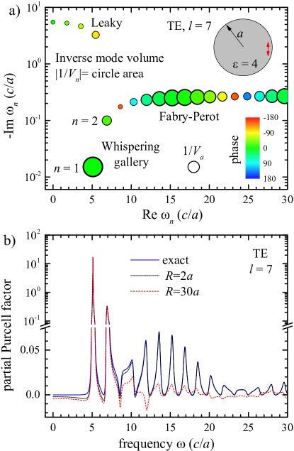
Figure 1: (color online) a) Mode volumes for a dielectric sphere in vacuum, with permittivity $\varepsilon=4$ and radius $a$, for $l=7$ TE modes and a point dipole placed at $|\mathbf{r}_{d}|=0.9a$ with direction ${\bf e}=(0,0,1)$ in spherical coordinates (see sketch). The mode volume is presented as the sum of the inverse mode volume over all degenerate states $m=-l,\dots,l$. Its amplitude is shown by the circle area and its phase by the color. The volume of the sphere $V_{a}=4\pi a^{3}/3$ is shown for comparison. The position of the circles in the complex frequency plane is given by the mode eigenfrequency $\omega_{n}$. b) Partial Purcell factor calculated via Eq. (9) for $l=7$ and TE polarization, for the geometry of a), using the exact mode normalization (blue line) and the LK normalization evaluated for integration volumes given by a sphere of radius $R=2a$ and $R=30a$, as labeled.

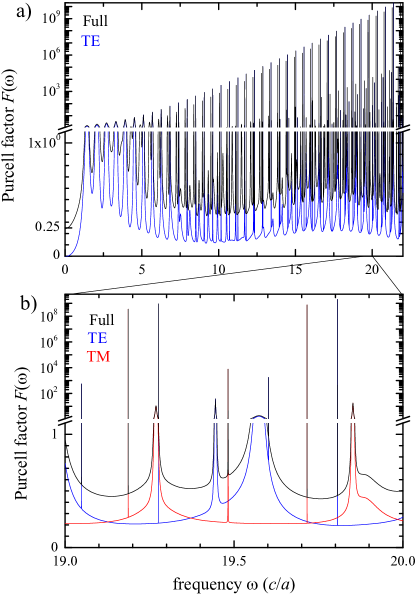
Figure 2: (color online) Purcell factor versus transition frequency $\omega$ calculated by Eq. (9) using modes with $l<38$ and $|\omega_{n}|<40c/a$. The dipole is placed at $|\mathbf{r}_{d}|=0.9a$ as in Fig. 1, and the PF is averaged over the polarization directions. a) Full PF (black line) and partial PF for TE modes only (blue line). b) zoom of a), showing additionally the partial PF for TM modes (red line).

For illustration, we have calculated the mode volume and PF of a dielectric spherical resonator with homogeneous permittivity ($\varepsilon=4$) surrounded by vacuum, for a point dipole placed at $|\mathbf{r}_{d}|=0.9a$ with direction ${\bf e}=(0,0,1)$ in spherical coordinates (see sketch in Fig. 1a). The inverse mode volume of several eigenmodes with the angular momentum $l=7$ and transverse electric (TE) polarization, summed over the degenerate states with azimuthal number $m=-l,\dots,l$, is shown in Fig. 1a. The modes can be classified as leaky modes, whispering gallery modes (WGMs), and Fabry-Pérot (FP) modes, as indicated. The chosen dipole position is close to the field maximum of the fundamental WGM, therefore its mode volume is small and essentially real. With increasing mode order going into the FP modes, the mode volume oscillates as the field maxima and minima move across the dipole position. Interestingly, the phase of the mode volume rotates accordingly, yielding negative mode volumes at the positions of the field minima, at which the mode field is imaginary. This also elucidates that the radiative decay into the modes is not a simple superposition of Lorentzian lines describing independent channels, but shows interference. This can actually be expected, as modes of equal $l$, $m$, and polarization couple into the same outgoing loss channel.

The resulting partial PF for $l=7$ TE modes (see Fig. 1b) is dominated by the $n=1$ WGM providing on resonance a PF of about 20. The complex mode volume leads to non-Lorentzian features in the spectrum, due to the mode interference. The total contribution to the PF of all modes for each loss channel (for spherical symmetry all modes with equal $m$, $l$, and polarization) is strictly positive, as expected. To exemplify the issues with the LK normalization, we show the resulting PF for two finite integration volumes given by spheres of radius $R=2a$ and $R=30a$. The observed deviation, which is increasing with $R$, is showing an underestimation of the contribution of leaky and FP modes. The PF also shows negative values which are unphysical. Taking the limit $R\to\infty$, the mode volume diverges exponentially, according to Eq. (4), see Fig. S1 of Ref. SM , – this is also true for high-Q modes but commences at larger $R$ – so that the PF vanishes. In metallic resonators the modes have generally low Q-factors, yielding a fast exponential growth (see Fig. S2) and large errors of Eq. (4) for any $\cal V$.

To explicitly show the validity of the spectral representation and the resulting PF based on the exact normalization, we compare it with the PF calculated using the analytic GF of a sphere. We take into account both TE and transverse magnetic (TM) polarizations and sum over all significant values of $l$ and $m$. Examples of mode volumes and partial PFs for the TM modes are shown in Figs. S3 and S4 of Ref. SM for two different directions of the dipole. The resulting PF for a dipole at a distance $0.9a$ from the center of the sphere averaged over its polarization directions is shown in Fig. 2, with partial PFs shown separately for TE modes in Figs. 2(a) and 2(b) and for TM modes in Fig. 2(b). In the low-frequency limit the well known static value of the field reduction by a factor of $3/(2+\varepsilon)$ inside a dielectric sphere in vacuum is reproduced, so that $F(0)=0.25$. Comparing these results with the ones obtained using the analytic GF of a sphere shows excellent agreement, as detailed in Sec. VI of Ref. SM . The spectral zoom in Fig. 2(b) allows to see the extremely sharp WGM lines on top of much wider resonances and their separation into TE and TM modes. Purcell factors up to $10^{10}$ are found in resonance to WGM of similarly high Q-factors.

In conclusion, we have provided a general exact analytic form of the normalization of eigenmodes in an arbitrary open optical resonator, which rectifies a normalization expression previously believed to be valid. We have shown that the normalization can be used with high accuracy also for RSs determined by numerical solvers, while at the same time the flexible normalization volume does not constrain the size of the computational domain. The correct normalization is of key importance for the electromagnetic theory, as it determines the spectral representation of the dyadic Green’s function of Maxwell’s wave equation, which can be used for calculation of any observable, such as scattering and extinction cross-sections and local density of states. We focussed in the present work on the consequences for the determination of the mode volume and the Purcell factor, which is a cornerstone for cavity quantum electrodynamics and nanoplasmonics. Further fundamental developments enabled by this exact normalization are to be expected, as exemplified by the rigorous perturbation theory in electrodynamics called the resonant-state expansion  MuljarovEPL10 ; DoostPRA12 ; DoostPRA13 ; ArmitagePRA14 ; DoostPRA14 .

- (1) E. M. Purcell, Phys. Rev. 69, 681 (1946).
- (2) R. Coccioli et al., IEE Proc.-Optoelectron. 145, 391 (1998).
- (3) For consistency with results of the present paper, we have removed from the original formula the factor of and added the dipole polarization vector .
- (4) P. Kristensen, C. van Vlack, and S. Hughes, Opt. Lett. 37, 1649 (2012).
- (5) P. T. Kristensen and S. Hughes, ACS Photonics 1, 2 (2014).
- (6) P. T. Leung, S. Y. Liu, and K. Young, Phys. Rev. A 49, 3982 (1994).
- (7) P. T. Leung and K. M. Pang, J. Opt. Soc. Am. B 13, 805 (1996).
- (8) E. A. Muljarov, W. Langbein, and R. Zimmermann, Europhys. Lett. 92, 50010 (2010).
- (9) M. B. Doost, W. Langbein, and E. A. Muljarov, Phys. Rev. A 85, 023835 (2012).
- (10) M. B. Doost, W. Langbein, and E. A. Muljarov, Phys. Rev. A 87, 043827 (2013).
- (11) L. J. Armitage, M. B. Doost, W. Langbein, and E. A. Muljarov, Phys. Rev. A 89, 053832 (2014).
- (12) M. B. Doost, W. Langbein, and E. A. Muljarov, Phys. Rev. A 90, 013834 (2014).
- (13) R. J. Glauber and M. Lewenstein, Phys. Rev. A 43, 467 (1991).
- (14) H. T. Dung, L. Knöll, and D.-G. Welsch, Phys. Rev. A 62, 053804 (2000).
- (15) H. T. Dung, L. Knöll, and D.-G. Welsch, Phys. Rev. A 64, 013804 (2001).
- (16) Q. Bai et al., Opt. Express 21, 27371 (2013).
- (17) C. Sauvan, J. P. Hugonin, I. S. Maksymov, and P. Lalanne, Phys. Rev. Lett. 110, 237401 (2013).
- (18) M. Agio and D. M. Cano, Nat. Photon. 7, 674 (2013).
- (19) Supplemental Material.
- (20) H. Levine and J. Schwinger, Commun. Pure Appl. Math 3, 355 (1950).