Imperial/TP/2014/JG/04

The thermoelectric properties of
inhomogeneous holographic lattices

Aristomenis Donos¹ and Jerome P. Gauntlett²

¹DAMTP, University of Cambridge
Cambridge, CB3 0WA, U.K.

²Blackett Laboratory, Imperial College
London, SW7 2AZ, U.K.

Abstract

We consider inhomogeneous, periodic, holographic lattices of $D=4$ Einstein-Maxwell theory. We show that the DC thermoelectric conductivity matrix can be expressed analytically in terms of the horizon data of the corresponding black hole solution. We numerically construct such black hole solutions for lattices consisting of one, two and ten wave-numbers. We numerically determine the AC electric conductivity which reveals Drude physics as well as resonances associated with sound modes. No evidence for an intermediate frequency scaling regime is found. All of the monochromatic lattice black holes that we have constructed exhibit scaling behaviour at low temperatures which is consistent with the appearance of $AdS_{2}\times\mathbb{R}^{2}$ in the far IR at $T=0$.

1 Introduction

In considering possible applications of holography to real world systems, the electrical conductivity is an interesting observable to focus on. Indeed many exotic materials, which are known to be strongly coupled, exhibit striking and poorly understood phenomena. For example, the strange metallic phase, arising in the cuprates and heavy fermion systems, has a DC resistivity which scales linearly in temperature, in contrast to ordinary Fermi liquids were it scales quadratically.

For systems at finite charge density, the electric and heat currents mix and so one should consider the thermoelectric conductivity matrix. The electrically charged AdS-RN black holes of Einstein-Maxwell theory provide a natural starting point to investigate thermoelectric conductivities using holography. These black holes describe CFTs at finite charge density with unbroken translation invariance. However, the latter implies that momentum is conserved and hence the application of an external electric field gives rise to infinite thermoelectric DC conductivities. More precisely, the real part of the AC conductivity has a delta function for all temperatures [1, 2, 3]. In order to alleviate this feature one needs a mechanism to dissipate momentum. This can be achieved by considering “holographic lattice” black holes where one explicitly breaks the translation invariance using UV deformations[4, 5, 6, 7, 8, 9, 10, 11, 12, 13].

Recently it has been shown how to obtain the thermoelectric DC conductivity in terms of black hole horizon data for a general class of homogeneous Q-lattices [12, 14]. Recall that Q-lattices exploit a global symmetry in the bulk space-time in order to break translation invariance while maintaining a homogeneous metric [10]. At a technical level this is significant because the holographic black holes can be constructed by solving ODEs rather than PDEs, and this simplification helped in obtaining the results in [12, 14]. The basic strategy of [12, 14] is to consider linearised perturbations about the black holes with sources for the electric and heat currents that are linear in time. By then manipulating the equations of motion to obtain expressions for the electric and heat currents in terms of horizon data, and also demanding regularity of the perturbation at the black hole horizon, leads to the final result.

In the first part of this paper we show that the techniques of [12, 14] can also be applied in the context of inhomogeneous holographic latices. More specifically we obtain an analytic result for the thermoelectric DC conductivity for holographic lattices associated with an arbitrary periodic chemical potential depending on one of the spatial coordinates, in the context of $D=4$ Einstein-Maxwell theory. Our final results, which are summarised in section (3.3), are remarkably similar to those obtained in [12, 14]. In particular, the electric DC conductivity is naturally written as a sum of two terms, one of which is precisely the electric conductivity with vanishing heat current and hence can be thought of, loosely, as being associated with the evolution of charged particle-hole pairs (possibly pair produced). The other term can be thought of as arising from momentum dissipation processes. We also find a result for the “figure of merit” $ZT$, which provides a measure of the efficiency of a thermoelectric engine (e.g. see [26]), and show that it can become arbitrarily large at low temperatures (the maximum known value for real materials is less than three.)

We also find in the high temperature limit that the electrical DC conductivity saturates to a constant value, set by the details of the UV deformation, generically with $\sigma>1$. This saturation of the DC conductivity is reminiscent of the Mott-Ioffe-Regel bound [27, 28] of real metals, but here it is arising in a strongly coupled setting. Note, by contrast, that the $T\to\infty$ limit of the electrical conductivity for the Q-lattices diverges, except in the special case that the UV deformation is a marginal operator as in [11], for example.

In the second part of this paper we construct fully back reacted black hole solutions of $D=4$ Einstein-Maxwell theory corresponding to various holographic lattices by numerically solving PDEs. We will consider monochromatic lattices with a single wave-number $k$ as well as dichromatic lattices with wave-numbers $k$ and $2k$ with the same phase. We also consider an example of a “dirty lattice” built from many wave-numbers (ten) and random phases. In the monochromatic case, such black holes were first constructed in [5], building on the pioneering work [4] and while we recover many of the results of that paper, we also find some important differences. We will calculate the optical conductivity and observe the appearance of Drude-type peaks that are broadly similar to what was seen in [5]. We use our AC results to obtain the limiting DC conductivity and we find excellent agreement (better than $10^{-4}\%$) when we compare with the results using our new analytic formula. This provides an excellent test of our numerics and the fit to Drude physics.

A striking claim of [4, 5] was the existence of an intermediate frequency scaling regime for the optical conductivity for various holographic lattices, including the lattices we will construct here. More precisely, for the monochromatic case, the optical conductivity was reported to have the form $|\sigma(\omega)|\sim B\omega^{-2/3}+C$, where $B,C$ are frequency independent constants within the range $2<\omega\tau<8$, where $\tau$ is the characteristic time scale obtained from the Drude peak. Since similar behaviour is seen for the high $T_{c}$ cuprate superconductors, albeit with $C=0$ and a frequency independent phase (e.g. [29, 30]), it is important to further investigate this issue. The experimental data is plotted on a log-log diagram and, similar looking plots were presented in [4, 5], based on their results for the AC conductivity. While we find some discrepancy with the AC conductivity plots in [5] a more important point is that if such an intermediate power-law is present it should be manifest using more refined measures. In [10], it was suggested that a sharp diagnostic for such intermediate scaling is to plot the quantity $1+(\omega/\mu)|\sigma|^{\prime\prime}/|\sigma|^{\prime}$ and look for a range of $\omega/\mu$ in which this quantity is constant. Doing this we will find no evidence for such an intermediate scaling regime for the black holes that we construct here. Indeed, the intermediate behaviour for the optical conductivity is broadly similar to what was seen for the homogeneous Q-lattices constructed in [10].

At very low temperatures, all of the black holes associated with monochromatic lattices that we have constructed appear to approach $AdS_{2}\times\mathbb{R}^{2}$ in the far IR. More precisely, as $T\to 0$ the DC conductivity of the black holes exhibit a scaling behaviour consistent with the $T=0$ black holes being domain walls interpolating between an irrelevant deformation of $AdS_{2}\times\mathbb{R}^{2}$ in the far IR and $AdS_{4}$ in the UV, as first envisaged by [31]. We find no evidence for the new “floppy” ground states that were discussed in [32]; it is logically possible that they appear at even lower temperatures than what we have considered, but the robustness of the scaling behaviour makes this seem unlikely to us. It is an open possibility whether stronger lattice deformations than we have constructed and/or different types of lattice deformations will lead to a transition to new IR behaviour, as in the metal-insulator transitions of [7, 10, 12] or the metal-metal transitions of [12].

The plan of the rest of the paper is as follows. In section 2 we describe the inhomogeneous lattice black holes of Einstein-Maxwell theory that we will be considering. The derivation of the thermoelectric DC conductivity is presented in section 3. For readers who are just interested in the final analytic results, we point them to sections 3.3 and the subsequent discussion in section 3.4. In section 4, following the approach of [33], we describe the numerical methodology that we employ to solve the PDEs which leads to the holographic lattice black holes. We also explain how we obtain the AC conductivity. The main results of our numerical constructions are presented in section 4.3. We show that the electrical conductivity satisfies a standard type of sum rule, following [34], and a second sum rule which is associated with the electromagnetic duality of the $D=4$ Einstein-Maxwell theory [35]. We briefly conclude in section 5. We have three appendices. In appendix A we discuss the derivation of the stress tensor and heat current, while appendix B describes some aspects of the implementation of our numerics as well as some of the convergence checks that we used. In appendix C we make some additional comments on the relation of our work to that of [32].

2 Inhomogeneous lattices

We will focus on Einstein-Maxwell theory in four bulk dimensions, which is a minimal and rather universal setting to study holographic lattices. In particular, it can be obtained as a consistent Kaluza-Klein truncation associated with an arbitrary $AdS_{4}\times M$ solution of string/M-theory, where $M$ is a compact manifold with an isometry. An interesting class of examples is provided by the infinite class of $AdS_{4}\times SE_{7}$ solutions, where $SE_{7}$ is a seven-dimensional Sasaki-Einstein space, dual to CFTs with $N=2$ supersymmetry in $d=3$ space-time dimensions [36].

The action is given by

$$S=\int d^{4}x\sqrt{-g}\,\left(R+6-\frac{1}{4}\,F^{2}\right)\,,$$ (2.1)

with $F=dA$ being the field strength of the gauge field $A$ and $F^{2}=F_{\mu\nu}F^{\mu\nu}$. The equations of motion can be written in the form

$$E_{\mu\nu}\equiv R_{\mu\nu}+{3}g_{\mu\nu}-\frac{1}{2}\left(F_{\mu\rho}F_{\nu}{}^{\rho}-\frac{1}{4}g_{\mu\nu}\,F^{2}\right) =0\,,$$

$$\nabla_{\mu}F^{\mu\nu} =0\,.$$ (2.2)

Note that we have chosen the cosmological constant so that a unit radius $AdS_{4}$ solves the equations of motion. We have also set $16\pi G=1$ in order not to clutter up various equations.

The electrically charged AdS Reissner-Nordström (AdS-RN) black brane solution solves the equations of motion and is the bulk dual of a CFT held at temperature $T$ and deformed by a constant chemical potential $\mu$. Recall that at $T=0$ the solution interpolates between $AdS_{4}$ in the UV and the electrically charged $AdS_{2}\times\mathbb{R}^{2}$ solution in the IR. The AdS-RN black hole preserves translation invariance and hence there is no mechanism for momentum to dissipate upon adding an external electric field. This gives rise to infinite DC conductivity, or more precisely a delta function in the optical conductivity at zero frequency. This feature can be eliminated by studying more general black holes in which the chemical potential has a periodic dependence on one of the spatial dimensions, $x$, with period $L$. We can write

$$\mu\left(x\right)=\mu_{0}+\bar{\mu}\left(x\right)\,,$$ (2.3)

with $\mu_{0}$ a constant, and $\bar{\mu}\left(x\right)=\bar{\mu}\left(x+L\right)$ is a periodic function which averages to zero over a period. Note that when $\mu_{0}\neq 0$, a simple scaling argument reveals that true UV parameters are $T/\mu_{0}$ combined with the function $\bar{\mu}\left(x/\mu_{0}\right)/\mu_{0}$ with period $L\,\mu_{0}$. We also note that in the figures that appear later in the paper we have dropped the subscript from $\mu_{0}$ for clarity.

Some special examples of these holographic lattice black holes have been studied previously, for the special case of monochromatic sources. Specifically, black holes associated with deformations of the form $\mu=\mu_{0}+V\cos(kx)$ were constructed for $\mu_{0}\neq 0$ in [5] (and will be reconstructed here in section 4.1) and for $\mu_{0}=0$ in [9]. In the $T=0$ limit the black holes with $\mu_{0}\neq 0$ in [5] approach $AdS_{2}\times\mathbb{R}^{2}$ in the far IR, perturbed by irrelevant deformations, and we will find the same feature here (in contrast to the more recent claims of [32]), while those with $\mu_{0}=0$ that were constructed in [9] approach $AdS_{4}$.

Our new analytic results for the DC thermoelectric conductivity, described in the next subsections, will be valid for an arbitrary periodic chemical potential deformation of the form (2.3). An ansatz that is general enough to cover the relevant black hole solutions of interest is given by

$$ds^{2} =-U\,H_{tt}\,dt^{2}+\frac{H_{rr}}{U}\,dr^{2}+\Sigma\,\left[e^{B}dx^{2}+e^{-B}\,dy^{2}\right]\,,$$

$$A =a_{t}\,dt\,,$$ (2.4)

where $U=U(r)$, while $H_{tt},H_{rr},\Sigma,e^{B}$ and $a_{t}$ are all functions of both $r$ and $x$.

The boundary conditions at the asymptotic $AdS_{4}$ boundary, which we take to be located at $r\to\infty$, are given by $U,\Sigma\to r^{2}$, $H_{tt},H_{rr},e^{B}\to 1$ and $a_{t}\to\mu\left(x\right)$ as in (2.3). The black hole horizon is taken to be located at $r=0$ and regularity of the solution implies that we can expand the functions in powers of $r$ as

$$U\left(r\right) =4\pi\,T\,r+U^{(2)}\left(x\right)r^{2}+\dots\,,$$

$$a_{t}(r,x) =r\left(a^{(0)}_{t}\left(x\right)+a^{(1)}_{t}\left(x\right)r+\dots\right)\,,$$

$$H_{tt}(r,x) =H^{(0)}_{tt}\left(x\right)+H_{tt}^{(1)}\left(x\right)r+\dots\,,$$

$$H_{rr}(r,x) =H^{(0)}_{tt}\left(x\right)+H_{rr}^{(1)}\left(x\right)r+\dots\,,$$

$$\Sigma(r,x) =\Sigma^{(0)}\left(x\right)+\Sigma^{(1)}\left(x\right)r+\dots\,,$$

$$B(r,x) =B^{(0)}\left(x\right)+B^{(1)}\left(x\right)r+\dots\,,$$ (2.5)

where $a^{(0)}_{t},H^{(0)}_{tt},\Sigma^{(0)}$ and $B^{(0)}$ are all periodic functions of $x$, as are the higher order terms in the expansion in $r$. Indeed, regularity of the solutions as $r\to 0$ is easily seen by replacing the $t$ coordinate with the in-going Eddington-Finklestein coordinate $v$ defined by

$$v=t+(4\pi T)^{-1}\ln r+\mathcal{O}(r)\,.$$ (2.6)

The current density $J^{a}\equiv\{J^{t},J^{x},J^{y}\}$ in the dual field theory takes the form

$$J^{a}=\sqrt{-g}F^{ar}\,,$$ (2.7)

where the right hand-side is evaluated at the boundary $r\to\infty$. With this definition $J^{a}$ has a finite limit as $r\to\infty$ (see the discussion in appendix A). The total constant charge, $q$, of the background black holes is given by $q\equiv\int J^{t}$, where we have introduced the notation

$$\int\qquad\leftrightarrow\qquad L^{-1}\,\int_{0}^{L}dx\,,$$ (2.8)

with $L$ the period of $x$. We can obtain an expression for $q$ in terms of horizon data by using the gauge-equations of motion. Indeed the only non-zero component of the gauge-field equation of motion is the $t$ component which we can write as $\sqrt{-g}\nabla_{\mu}F^{\mu t}=\partial_{r}(\sqrt{-g}F^{rt})+\partial_{x}(\sqrt{-g}F^{xt})=0$. Since $\sqrt{-g}F^{xt}$ depends on $\partial_{x}a_{t}$, after integrating over a period of $x$ the second-term vanishes and we deduce that

$$q =\int\frac{\Sigma\partial_{r}a_{t}}{(H_{rr}H_{tt})^{1/2}}\,,$$

$$=\int\frac{\Sigma^{(0)}a^{(0)}_{t}}{H_{tt}^{(0)}}\,,$$ (2.9)

where the second line follows by evaluating the constant at the horizon.

3 The thermoelectric DC conductivity

3.1 Calculating $\sigma$ and $\bar{\alpha}$

In this subsection we calculate the DC conductivities associated with switching on a constant electric field on the boundary theory in the $x$ direction, the direction in which the background lattice breaks translational invariance. Recall, by definition, that the linear response is given by

$$J=\sigma E,\qquad Q=\bar{\alpha}TE\,,$$ (3.1)

where $J\equiv J^{x}$ is the electric current and $Q\equiv T^{tx}-\mu J$ is the heat current, both in the $x$ direction, and $\sigma$, $\bar{\alpha}$ are the electric and thermoelectric DC conductivities. We will show how $\sigma$, $\bar{\alpha}$ can be expressed in terms of horizon data of the unperturbed black hole.

We first introduce gauge field perturbations of the form

$$\delta A=\delta a_{\mu}(r,x)dx^{\mu}-E\,t\,dx\,,$$ (3.2)

where $E$ is the constant magnitude of the linearised electric field in the $x$ direction and $\delta a_{\mu}$, whose non-vanishing components lie in the set $\left\{\delta a_{t},\delta a_{r},\delta a_{x}\right\}$, are functions of $r,x$ and are periodic in $x$. This is supplemented with metric perturbations $\delta g_{\mu\nu}$, with non-vanishing components lying in the set $\left\{\delta g_{tt},\delta g_{tr},\delta g_{rr},\delta g_{rx},\delta g_{xx},\delta g_{tx},\delta g_{yy}\right\}$, which are again functions of $r,x$ and again are periodic in $x$. It will be convenient to not fully fix our gauge and coordinate dependence apart from requiring that some components fade sufficiently fast close to the $AdS_{4}$ boundary.

The next step is to use the equation of motion for the gauge-field to show that $J$ is constant and moreover to obtain an expression in terms of horizon data. Specifically, the $r$ and the $x$ components of the gauge field equation of motion imply that $\partial_{x}(\sqrt{-g}F^{xr})=0$ and $\partial_{r}(\sqrt{-g}F^{rx})=0$, respectively, and hence $J=\sqrt{-g}F^{xr}$ is a constant. Thus, we can write

$$J=\frac{e^{-B}}{\sqrt{H_{rr}H_{tt}}}\,\left[\partial_{x}a_{t}\delta g_{tr}-\partial_{r}a_{t}\delta g_{tx}+H_{tt}U\left(\partial_{x}\delta a_{r}-\partial_{r}\delta a_{x}\right)\right]\,,$$ (3.3)

where the right hand side can be evaluated at any value of $r$, including at the black hole horizon.

The next key step is to obtain a similar result for the heat current in the $x$ direction, $Q$, induced by $E$. Following [14] we first observe that if $k$ is any Killing vector satisfying $L_{k}F=0$, then we can define a two-form $G$ by

$$G^{\mu\nu}=\nabla^{\mu}k^{\nu}+\frac{1}{2}k^{[\mu}F^{\nu]\sigma}A_{\sigma}+\frac{1}{4}({\psi}-2\theta)F^{\mu\nu}\,,$$ (3.4)

where $\psi$ and $\theta$ are defined by $L_{k}A=d\psi$ and $i_{k}F=d\theta$. The two-form $G$ has the important property that

$$\nabla_{\mu}G^{\mu\nu}={3}k^{\nu}\,,$$ (3.5)

when the equations of motion (2) are satisfied (see appendix B of [14]). Focussing on the Killing vector $k=\partial_{t}$, if we consider the $r$ and $x$ components of (3.5) we deduce that $\partial_{x}(\sqrt{-g}G^{xr})=\partial_{r}(\sqrt{-g}G^{rx})=0$ and hence that $\sqrt{-g}G^{rx}$ is a constant. Choosing $\theta=-EX-a_{t}-\delta a_{t}$ and $\psi=-Ex$, we conclude that at linearised order we can write

$$Q \equiv 2\sqrt{-g}G^{rx}\,,$$

$$=2\sqrt{-g}\nabla^{r}k^{x}+a_{t}\sqrt{-g}F^{rx}\,,$$

$$=\frac{e^{-B}U^{2}H_{tt}^{3/2}}{\sqrt{H_{rr}}}\,\Bigg{[}\partial_{r}\left(\frac{\delta g_{tx}}{UH_{tt}}\right)-\partial_{x}\left(\frac{\delta g_{tr}}{UH_{tt}}\right)\Bigg{]}-a_{t}J\,,$$ (3.6)

and we can evaluate the right hand side at any value of $r$. In particular, if we evaluate at the boundary $r\to\infty$ we find, as we explain in appendix A,

$$Q=(T^{tx}-\mu J)\,.$$ (3.7)

To proceed we now need to ensure that the perturbation is regular at the horizon, after switching to the Eddington-Finklestein coordinate $v$ given in (2.6). Near $r=0$ we demand that we can expand

$$\delta g_{tt} =U\left(r\right)\,\left(\delta g^{(0)}_{tt}\left(x\right)+{\cal O}(r)\right),\quad\delta g_{rr}=\frac{1}{U}\,\left(\delta g_{rr}^{(0)}\left(x\right)+{\cal O}(r)\right),$$

$$\delta g_{tr} =\delta g_{tr}^{(0)}\left(x\right)+{\cal O}(r),\quad\delta g_{xx}=\delta g_{xx}^{(0)}\left(x\right)+{\cal O}(r),\quad\delta g_{yy}=\delta g_{yy}^{(0)}\left(x\right)+{\cal O}(r)\,,$$

$$\delta g_{tx} =e^{B^{(0)}}\,\left(\delta g_{tx}^{(0)}\left(x\right)+{\cal O}(r)\right),\quad\delta g_{rx}=\frac{e^{B^{(0)}\left(x\right)}}{U}\,\left(\delta g_{rx}^{(0)}\left(x\right)+{\cal O}(r)\right)\,,$$

$$\delta a_{t} =\delta a_{t}^{(0)}\left(x\right)+{\cal O}(r),\quad\delta a_{r}=\frac{1}{U}\,\left(\delta a_{r}^{(0)}\left(x\right)+{\cal O}(r)\right)\,,$$

$$\delta a_{x} =\ln{U}\,\delta a_{x}^{(0)}\left(x\right)+{\cal O}(r)\,,$$ (3.8)

with the following constraints on the leading functions of $x$:

$$\delta g_{tt}^{(0)}+\delta g_{rr}^{(0)}-2\,\delta g_{rt}^{(0)}=0,\qquad\delta g^{(0)}_{rx}=\delta g^{(0)}_{tx}\,,$$

$$\delta a_{r}^{(0)}=\delta a_{t}^{(0)},\qquad\delta a_{x}^{(0)}=-\frac{E}{4\pi\,T}\,.$$ (3.9)

Observe, in particular, that the expression for $\delta a_{x}^{(0)}$ involving the UV data $E$ arises as a direct consequence of the way in which we switched on the background electric field in (3.2).

Expanding out the right hand side of (3.3) at the black hole horizon we find that at leading order in $r$ we must have

$$J=e^{-B^{(0)}}\left(E+\partial_{x}\delta a^{(0)}_{t}\right)-\frac{\,a^{(0)}_{t}}{H^{(0)}_{tt}}\delta g^{(0)}_{tx}\,,$$ (3.10)

where the right hand side must be a constant. We can also evaluate the right hand side of the expression for $Q$ in (3.1) at the horizon. At leading order in $r$ we deduce that

$$Q=-4\pi T\delta g_{tx}^{(0)}\,,$$ (3.11)

and hence we obtain the important condition

$$\delta g_{tx}^{(0)}=constant\,.$$ (3.12)

By expanding to next order in $r$, at fixed temperature, we obtain another constraint on the horizon boundary data:

$$\partial_{x}\,\left(4\pi T\,\frac{\delta g_{tr}^{(0)}}{H_{tt}^{(0)}}\right)+\frac{a_{t}^{(0)}}{H_{tt}^{(0)}}\,\left(E+\partial_{x}\delta a^{(0)}_{t}\right)$$

$$+\frac{\delta g_{tx}^{(0)}}{(H_{tt}^{(0)})^{2}}\left((a_{t}^{(0)})^{2}+2\pi T\left(H_{rr}^{(1)}+2H_{tt}^{(0)}B^{(1)}-3H_{tt}^{(1)}\right)-2H_{tt}^{(0)}U^{(2)}\right)=0\,.$$ (3.13)

Remarkably, using the background equations of motion we can rewrite this in the following useful form

$$\partial_{x}\,\left(4\pi T\,\frac{\delta g_{tr}^{(0)}}{H_{tt}^{(0)}}-\frac{1}{\Sigma^{(0)}}\partial_{x}\left[B^{(0)}-\ln(H_{tt}^{(0)}\Sigma^{(0)})\right]\delta g_{tx}^{(0)}\right)$$

$$\qquad\qquad+\frac{a_{t}^{(0)}}{H_{tt}^{(0)}}\,\left(E+\partial_{x}\delta a^{(0)}_{t}\right)+\frac{1}{\Sigma^{(0)}}\,\left[\partial_{x}\ln{\frac{e^{B^{(0)}}}{\Sigma^{(0)}}}\right]^{2}\delta g_{tx}^{(0)}\,=0\,.$$ (3.14)

The constraints (3.1), (3.10), (3.12) and (3.1) are sufficient to get a consistent set of ODEs for the expansion parameters in the falloff (3.1). In particular, by expanding the right hand side of (3.3) and (3.1) in higher powers of $r$ at the black hole horizon do not lead to additional constraints.

We have now assembled the ingredients to obtain the DC conductivities $\sigma$ and $\bar{\alpha}$. We multiply equation (3.10) by $e^{B^{(0)}}$ and then integrate over a period of $x$ to obtain an equation involving $E$, $J$ and $\delta g_{tx}^{(0)}$. Equation (3.10) can also be used in (3.1) which we then integrate to give a relation between $J$ and $\delta g_{tx}^{(0)}$. We can solve for $J$ in terms of $E$, and hence obtain an expression for $\sigma=J/E$. We find

$$\sigma =\frac{\int\left(e^{B^{(0)}}\left(\frac{a_{t}^{(0)}}{H_{tt}^{(0)}}\right)^{2}+\frac{1}{\Sigma^{(0)}}\left[\partial_{x}\ln{\frac{e^{B^{(0)}}}{\Sigma^{(0)}}}\right]^{2}\right)}{\int e^{B^{(0)}}\int\left(e^{B^{(0)}}\left(\frac{a_{t}^{(0)}}{H_{tt}^{(0)}}\right)^{2}+\frac{1}{\Sigma^{(0)}}\left[\partial_{x}\ln{\frac{e^{B^{(0)}}}{\Sigma^{(0)}}}\right]^{2}\right)-\left(\int e^{B^{(0)}}\frac{a_{t}^{(0)}}{H_{tt}^{(0)}}\right)^{2}}\,,$$ (3.15)

where we remind the reader that the notation $\int$ means $L^{-1}\,\int_{0}^{L}dx$, with $L$ the period of $x$. As advertised this formula for $\sigma$ only depends on the near horizon data of the unperturbed black hole. The Schwarz inequality implies that

$$\left(\int e^{B^{(0)}}\frac{a_{t}^{(0)}}{H_{tt}^{(0)}}\right)^{2}\leq\int e^{B^{(0)}}\,\int e^{B^{(0)}}\,\left(\frac{a_{t}^{(0)}}{H_{tt}^{(0)}}\right)^{2}\,,$$ (3.16)

and hence we deduce that $\sigma>0$.

We also find an expression relating $Q=-4\pi T\delta g_{tx}^{(0)}$ and $E$ and we deduce that $\bar{\alpha}\equiv\frac{Q}{TE}$ can be written as

$$\bar{\alpha}=\frac{4\pi\int e^{B^{(0)}}\frac{a_{t}^{(0)}}{H_{tt}^{(0)}}}{\int e^{B^{(0)}}\int\left(e^{B^{(0)}}\left(\frac{a_{t}^{(0)}}{H_{tt}^{(0)}}\right)^{2}+\frac{1}{\Sigma^{(0)}}\left[\partial_{x}\ln{\frac{e^{B^{(0)}}}{\Sigma^{(0)}}}\right]^{2}\right)-\left(\int e^{B^{(0)}}\frac{a_{t}^{(0)}}{H_{tt}^{(0)}}\right)^{2}}\,.$$ (3.17)

3.2 Calculating $\bar{\kappa}$ and $\alpha$

In this section we will introduce a source for the heat current. Following [14] we consider the following time dependent perturbation around the background (2):

$$\delta ds^{2} =\delta g_{\mu\nu}\,dx^{\mu}\,dx^{\nu}-2t(UH_{tt}\zeta)\,dt\,dx\,,$$

$$\delta A =\delta a_{\mu}\,dx^{\mu}+t(a_{t}\,\zeta)dx\,.$$ (3.18)

The non-zero static perturbations are in the sets $\left\{\delta g_{tt},\delta g_{tr},\delta g_{rr},\delta g_{rx},\delta g_{xx},\delta g_{tx},\delta g_{yy}\right\}$ and $\left\{\delta a_{t},\delta a_{r},\delta a_{x}\right\}$ and they depend on $r$ and periodically on $x$. It is important to emphasise that the terms that are linear in $t$, parametrised by $\zeta$, have been chosen so that all time dependence drops out after we substitute into the equations of motion. As discussed in [14] they provide a source for the heat current.

The near horizon expansion for the perturbation is very similar to (3.1)

$$\delta g_{tt} =U\left(r\right)\,\left(\delta g^{(0)}_{tt}\left(x\right)+{\cal O}(r)\right),\quad\delta g_{rr}=\frac{1}{U}\,\left(\delta g_{rr}^{(0)}\left(x\right)+{\cal O}(r)\right),$$

$$\delta g_{tr} =\delta g_{tr}^{(0)}\left(x\right)+{\cal O}(r),\quad\delta g_{xx}=\delta g_{xx}^{(0)}\left(x\right)+{\cal O}(r),\quad\delta g_{yy}=\delta g_{yy}^{(0)}\left(x\right)+{\cal O}(r)\,,$$

$$\delta g_{tx} =e^{B^{(0)}}\,\left(\delta g_{tx}^{(0)}\left(x\right)+\delta g_{tx}^{(l)}\left(x\right)\,U\,\ln U+{\cal O}(r)\right),\quad\delta g_{rx}=\frac{e^{B^{(0)}\left(x\right)}}{U}\,\left(\delta g_{rx}^{(0)}\left(x\right)+{\cal O}(r)\right)\,,$$

$$\delta a_{t} =\delta a_{t}^{(0)}\left(x\right)+{\cal O}(r),\quad\delta a_{r}=\frac{1}{U}\,\left(\delta a_{r}^{(0)}\left(x\right)+{\cal O}(r)\right)\,,$$

$$\delta a_{x} =\delta a_{x}^{(0)}\left(x\right)+{\cal O}(r)\,,$$ (3.19)

where once again regular in-falling boundary conditions require

$$\delta g_{tt}^{(0)}+\delta g_{rr}^{(0)}-2\,\delta g_{rt}^{(0)}=0,\qquad\delta g^{(0)}_{rx}=\delta g^{(0)}_{tx},\qquad\delta a_{r}^{(0)}=\delta a_{t}^{(0)}\,.$$ (3.20)

The extra logarithmic term appearing in the expansion of $\delta g_{tx}$ in (3.2), when compared to (3.1), is fixed by expanding the equations of motion of the fluctuations near the horizon at $r=0$. More specifically we find

$$\delta g_{tx}^{(l)}=-\frac{e^{-B^{(0)}}}{4\pi\,T}\,H_{tt}^{(0)}\,\zeta\,.$$ (3.21)

This is precisely of the form needed to make the perturbation regular after combining with the time dependent term in (3.2).

Once again we find that $J$, given by (3.3), is a constant. Furthermore, expanding the equations of motion close to the horizon we find once more that

$$\delta g_{tx}^{(0)}=constant\,,$$ (3.22)

$$J=e^{-B^{(0)}}\partial_{x}\delta a^{(0)}_{t}-\frac{\,a^{(0)}_{t}}{H^{(0)}_{tt}}\delta g^{(0)}_{tx}\,,$$ (3.23)

and

$$\partial_{x}\,\left(4\pi T\,\frac{\delta g_{tr}^{(0)}}{H_{tt}^{(0)}}-\frac{1}{\Sigma^{(0)}}\partial_{x}\left[B^{(0)}-\ln(H_{tt}^{(0)}\Sigma^{(0)})\right]\delta g_{tx}^{(0)}\right)$$

$$\qquad\qquad+\frac{a_{t}^{(0)}}{H_{tt}^{(0)}}\,\partial_{x}\delta a^{(0)}_{t}+\frac{1}{\Sigma^{(0)}}\,\left[\partial_{x}\ln{\frac{e^{B^{(0)}}}{\Sigma^{(0)}}}\right]^{2}\delta g_{tx}^{(0)}+4\pi T\,\zeta=0\,.$$ (3.24)

The expression for $Q$ given in (3.1) is again a constant and expanding near the horizon we have, as before,

$$Q=-4\pi T\delta g_{tx}^{(0)}\,.$$ (3.25)

As in [14] we find that the heat current has a time-independent piece, given by $Q$, and a time-dependent piece:

$$T^{tx}-\mu J^{x}=Q-\zeta tT^{xx}\,,$$ (3.26)

as we discuss in appendix A. As explained in appendix C of [14], the time-dependent piece is associated with a static susceptibility for the $Q$$Q$ correlator, given by $T^{xx}$ of the background. On the other hand the time independent piece is associated with the DC conductivity.

Using almost identical manipulations of the previous section we deduce the DC conductivities:

$$\alpha\equiv\frac{J}{T\zeta}=\frac{4\pi\int e^{B^{(0)}}\frac{a_{t}^{(0)}}{H_{tt}^{(0)}}}{\int e^{B^{(0)}}\int\left(e^{B^{(0)}}\left(\frac{a_{t}^{(0)}}{H_{tt}^{(0)}}\right)^{2}+\frac{1}{\Sigma^{(0)}}\left[\partial_{x}\ln{\frac{e^{B^{(0)}}}{\Sigma^{(0)}}}\right]^{2}\right)-\left(\int e^{B^{(0)}}\frac{a_{t}^{(0)}}{H_{tt}^{(0)}}\right)^{2}}\,,$$ (3.27)

and

$$\bar{\kappa}\equiv\,\frac{Q}{T\zeta}=\frac{(4\pi)^{2}T\int e^{B^{(0)}}}{\int e^{B^{(0)}}\int\left(e^{B^{(0)}}\left(\frac{a_{t}^{(0)}}{H_{tt}^{(0)}}\right)^{2}+\frac{1}{\Sigma^{(0)}}\left[\partial_{x}\ln{\frac{e^{B^{(0)}}}{\Sigma^{(0)}}}\right]^{2}\right)-\left(\int e^{B^{(0)}}\frac{a_{t}^{(0)}}{H_{tt}^{(0)}}\right)^{2}}\,.$$ (3.28)

Comparing with (3.17), it is satisfying that we have $\alpha=\bar{\alpha}$. Indeed this is expected since the lattice deformation does not break time-reversal invariance.

3.3 Summary of DC conductivity

We now summarise the results of the previous two subsections. To do so it is helpful to define the following quantity, constructed from the horizon data of the background black holes given in (2):

$$X=\int e^{B^{(0)}}\int\left(e^{B^{(0)}}\left(\frac{a_{t}^{(0)}}{H_{tt}^{(0)}}\right)^{2}+\frac{1}{\Sigma^{(0)}}\left[\partial_{x}\ln{\frac{e^{B^{(0)}}}{\Sigma^{(0)}}}\right]^{2}\right)-\left(\int e^{B^{(0)}}\frac{a_{t}^{(0)}}{H_{tt}^{(0)}}\right)^{2}\,,$$ (3.29)

where $\int$ is defined in (2.8). Using the Schwarz inequality (3.16) we have $X\geq 0$. The DC thermoelectric conductivities can then be written in the form:

$$\sigma =\frac{1}{\int e^{B^{(0)}}}+\frac{\left(\int e^{B^{(0)}}\frac{a_{t}^{(0)}}{H_{tt}^{(0)}}\right)^{2}}{X\int e^{B^{(0)}}}\,,$$

$$\bar{\alpha}=\alpha =4\pi\frac{\int e^{B^{(0)}}\frac{a_{t}^{(0)}}{H_{tt}^{(0)}}}{X}\,,$$

$$\bar{\kappa} =\frac{(4\pi)^{2}T\int e^{B^{(0)}}}{X}\,.$$ (3.30)

We have shown that these results are valid for all black hole solutions within the ansatz (2), with near horizon behaviour given by (2) and approaching $AdS_{4}$ in the UV with chemical potential $\mu(x)$. In fact we can show that they are also valid for more general black hole solutions provided that they have the same near horizon and asymptotic limits. For example, we have explicitly carried out the derivation for the black holes that we construct numerically in section 4 which have $g_{rx_{1}}\neq 0$.

We first observe that $\sigma$ and $\bar{\kappa}$ are both positive, as expected. We next note the similarity of these expressions with those obtained for the homogeneous lattices of [14]. In particular, the electric conductivity appears as the sum of two positive terms. The first term has a precise interpretation as the conductivity with zero heat current. Recalling the definition

$$\sigma_{Q=0}\equiv\left(\frac{J}{E}\right)_{Q=0}=\sigma-\frac{\alpha^{2}T}{\bar{\kappa}}\,,$$ (3.31)

which is guaranteed to be positive because it is proportional to the determinant of the positive definite thermo-electric matrix, we find

$$\sigma_{Q=0}=\frac{1}{\int e^{B^{(0)}}}\,.$$ (3.32)

Thus, very roughly, we can interpret the first term in $\sigma$ as being associated with the evolution of charged particle-hole pairs. The second term in $\sigma$ is then $\alpha^{2}T/\kappa$ which is obviously positive. For the special case of the neutral AdS Schwarzschild black hole the second term in $\sigma$ vanishes and the first term gives unity, and so we recover the result of [15]. For the AdS Schwarzschild black hole we will also have $\alpha=0$, but a divergent $\bar{\kappa}$ or, more precisely, a delta function in the AC thermal conductivity, since there is no momentum dissipation.

Observe that in general we have

$$\frac{\bar{\kappa}}{\alpha}=\frac{4\pi T\int e^{B^{(0)}}}{\int e^{B^{(0)}}\frac{a_{t}^{(0)}}{H_{tt}^{(0)}}}\,,$$ (3.33)

which is similar to an expression for the homogeneous lattices in [14], but unlike [14] the right-hand side is not simply given by $Ts/q$.

We next introduce $\kappa$, the thermal conductivity at zero electric current. We find

$$\kappa\equiv\bar{\kappa}-\frac{\alpha^{2}T}{\sigma} =\frac{(4\pi)^{2}T\int e^{B^{(0)}}}{X+\left(\int e^{B^{(0)}}\frac{a_{t}^{(0)}}{H_{tt}^{(0)}}\right)^{2}}\,.$$ (3.34)

We also obtain the following expressions for the Lorenz factors:

$$\bar{L} \equiv\frac{\bar{\kappa}}{\sigma T}=\frac{(4\pi)^{2}\left(\int e^{B^{(0)}}\right)^{2}}{X+\left(\int e^{B^{(0)}}\frac{a_{t}^{(0)}}{H_{tt}^{(0)}}\right)^{2}}\,,$$

$$L \equiv\frac{\kappa}{\sigma T}=\frac{(4\pi)^{2}\left(\int e^{B^{(0)}}\right)^{2}X}{\left[X+\left(\int e^{B^{(0)}}\frac{a_{t}^{(0)}}{H_{tt}^{(0)}}\right)^{2}\right]^{2}}\,.$$ (3.35)

Generically $L$, $\bar{L}$ are neither equal nor constant and the Wiedemann-Franz law is violated.

Finally we recall the definition of the dimensionless “figure of merit”, $ZT$,

$$ZT\equiv\frac{\alpha^{2}T}{\kappa\sigma}\equiv\frac{\alpha^{2}T}{\bar{\kappa}\sigma_{Q=0}}\,.$$ (3.36)

The figure of merit provides a measure of the efficiency of thermoelectric engines. There is no upper bound on $ZT$ and when $ZT$ approaches infinity the efficiency approaches the Carnot limit. The maximum value of $ZT$ for any known material is less than three. For our holographic lattice we find that

$$ZT=\frac{\left(\int e^{B^{(0)}}\frac{a_{t}^{(0)}}{H_{tt}^{(0)}}\right)^{2}}{X}\,.$$ (3.37)

We will see in the next subsection that holographic lattices can have arbitrarily high figures of merit at low temperatures.

3.4 High and low temperature behaviour

It is interesting to examine the high temperature behaviour of the DC conductivity. More precisely we are interested in the limit $T$ much greater than $\mu_{0}$ and $1/L$ where $\mu_{0}$ is the constant term in the modulated chemical potential (2.3) and $L$ is the period of the lattice. In this limit, the black hole background is approximated by the AdS-Schwarzschild black hole metric:

$$ds^{2}=-Udt^{2}+U^{-1}dr^{2}+r^{2}(dx^{2}+dy^{2})$$ (3.38)

with $U=r^{2}-r_{+}^{3}/r^{2}$ and $r_{+}=4\pi T/3$. Note that here the horizon is located at $r=r_{+}$ (and not at $r=0$ as above). Furthermore, in the high temperature limit the leading term in the solution for the gauge-field equations of motion is given by $a_{t}=(1-\frac{r_{+}}{r})\mu(x)$ for arbitrary periodic $\mu(x)$. Using (3.3) we obtain, as $T\to\infty$,

$$\sigma =1+\frac{(\int\mu)^{2}}{\int\mu^{2}-(\int\mu)^{2}}\,,\qquad\alpha=\frac{(4\pi)^{2}T}{3}\frac{\int\mu}{\int\mu^{2}-(\int\mu)^{2}}\,,$$

$$\bar{\kappa} =\frac{(4\pi)^{4}T^{3}}{9}\frac{1}{\int\mu^{2}-(\int\mu)^{2}}\,,\qquad\kappa=\frac{(4\pi)^{4}T^{3}}{9}\frac{1}{\int\mu^{2}}\,.$$ (3.39)

It is interesting that as $T\to\infty$ we have $\sigma$ approaching a constant value, with $\sigma\geq 1$ (recall that for the optical conductivity we have $\lim_{\omega\to\infty}\sigma(\omega)=1$). This is reminiscent of the Mott-Ioffe-Regel bound [27, 28] of metals (see figure 2), though here, of course, there are no quasi-particles.

We can also consider the low-temperature behaviour of the DC conductivity. This will obviously depend on the precise nature of the zero temperature ground states. As we will discuss in the next section, all of the black holes that we have constructed which are associated with monochromatic lattices with $\mu=\mu_{0}+V\cos(kx)$ and $\mu_{0}\neq 0$, seem to approach $AdS_{2}\times\mathbb{R}^{2}$ in the far IR at $T=0$, perturbed by an irrelevant deformation. For these black holes we can obtain the low-temperature behaviour as follows. We have $U\to 6r^{2}$, $H_{tt},H_{rr}\to 1$, $a^{(0)}_{t}\to 2\sqrt{3}$ and $e^{B_{0}},\Sigma$ approach constants that depend on the UV lattice data. We immediately conclude from (3.29) that $X\to 0$ and hence the second term in the DC electric conductivity in (3.3) dominates the first. More precisely, using the analysis of [31, 37] as $T\to 0$ we find that the DC conductivity scales as

$$\sigma\sim T^{2-2\Delta(\bar{k})},\quad\alpha\sim T^{2-2\Delta(\bar{k})},\quad\bar{\kappa}\sim T^{3-2\Delta(\bar{k})}\,,$$ (3.40)

where

$$\Delta(\bar{k})=\frac{1}{2}+\frac{1}{2}\left[5+4\bar{k}^{2}-4\sqrt{1+2\bar{k}^{2}}\right]^{1/2}\,,$$ (3.41)

and $\bar{k}$ is the renormalised wave-number, $\bar{k}\equiv k/(6\Sigma^{(0)}e^{B^{(0)}})^{1/2}$, which depends on the UV wave-number $k$ and the zero temperature domain wall solution. It is worth emphasising that for the $T=0$ AdS-RN black brane we have $\Sigma^{(0)}e^{B^{(0)}}=\mu^{2}/12$. Therefore we can define a length renormalisation factor, $\bar{\lambda}$, via

$$\bar{k}=\frac{k\sqrt{2}}{\mu\bar{\lambda}}$$ (3.42)

with, in general, $\bar{\lambda}\neq 1$ for the lattice black holes. As $T\to 0$ we note that the DC conductivity $\sigma$ diverges and this is associated with the Drude peak in the optical conductivity turning into a delta function at $T=0$. The scaling of $\sigma$, omitting the issue of $\bar{\lambda}$, was pointed out in [31], who obtained it in the limit of small lattice strengths by using the memory matrix formalism and also by taking a limit of the optical conductivity obtained from a matching argument. The issue of length renormalisation was discussed in [7, 10].

It is also interesting that we have the scaling $\kappa\sim T$. In particular, while $\kappa$ is going to zero, $\bar{\kappa}$ diverges if $\bar{k}^{2}>3/4+\sqrt{3}/2$, goes to a constant if $\bar{k}^{2}=3/4+\sqrt{3}/2$ and vanishes if $0\leq\bar{k}^{2}<3/4+\sqrt{3}/2$. We also note that as $T\to 0$ we have $\bar{L}\to\frac{4\pi^{2}}{3}=\frac{s^{2}}{q^{2}}$ and $\bar{\kappa}/\alpha\to Ts/q$, in this limit, independent of the lattice deformation. Finally, we note that the figure of merit is diverging as $T\to 0$ with $ZT\sim T^{2-2\Delta(\bar{k})}$.

Although we will not be discussing them further in this paper, we pause to comment upon the DC results for the lattices $\mu=\mu_{0}+V\cos(kx)$ with $\mu_{0}=0$ that were studied in [9]. In the $T=0$ limit these black holes approach $AdS_{4}$ in the far IR. It is straightforward to see that in the black hole solutions the $x$ dependence of the gauge field can be expanded in terms of Fourier modes that are odd multiples of $k$ whereas for the metric functions they will be even multiples. Hence, we can deduce that for these black holes we have, for all temperatures,

$$\sigma=\frac{1}{\int e^{B^{(0)}}}\,,\qquad\bar{\alpha}=\alpha=0\,,\qquad\bar{\kappa}=\frac{(4\pi)^{2}T}{\int\Big{(}e^{B^{(0)}}\left(\frac{a_{t}^{(0)}}{H_{tt}^{(0)}}\right)^{2}+\frac{1}{\Sigma^{(0)}}\left[\partial_{x}\ln{\frac{e^{B^{(0)}}}{\Sigma^{(0)}}}\right]^{2}\Big{)}}\,.$$ (3.43)

4 Numerical construction of inhomogeneous lattices and the AC conductivity

In this section we will numerically construct black holes corresponding to inhomogeneous lattices. We can then immediately obtain the DC conductivity using the results of the last section. We will also numerically determine the AC conductivity. We will see the appearance of a coherent Drude-type peak in the AC conductivity, as in [5], but we will not see any evidence for an intermediate scaling regime that was reported in [5]. On the other hand we observe see an interesting resonance phenomenon, also seen in [5], which we associate with sound modes. We also carry out a detailed check of a sum-rule satisfied by the optical conductivity and also a sum-rule associated with electromagnetic duality [35]. Finally, we show that the low temperature black holes exhibit scaling behaviour consistent with them approaching $AdS_{2}\times\mathbb{R}^{2}$ in the IR, in contrast to [32].

In section 4.1 and 4.2 we will describe the numerical construction and in section 4.3 we will present the main results.

4.1 The backgrounds

To construct the black hole geometries that we are interested in, we will make the following ansatz:

$$ds^{2} =\frac{1}{z^{2}}\left[-f\,Q_{tt}\,dt^{2}+\frac{Q_{zz}}{f}\,dz^{2}+Q_{xx}\,\left(dx+Q_{zx}\,dz\right)^{2}+Q_{yy}\,\,dy^{2}\right]\,,$$

$$A =\left(1-z\right)\,a_{t}\,dt\,,$$ (4.1)

where

$$f =\left(1-z\right)\,\left(1+z+z^{2}-\frac{\mu^{3}z^{3}}{4}\right)\,,$$ (4.2)

and $\mathcal{F}=\left\{Q_{tt},Q_{rr},Q_{xx},Q_{zx},Q_{yy},a_{t}\right\}$ are all functions of the radial coordinate $z$ and $x$. In this section, the $AdS_{4}$ boundary will be located at $z=0$ and the black hole horizon at $z=1$. Notice that the function $f$, with $Q_{tt}=Q_{rr}=Q_{xx}=Q_{yy}=1$, $Q_{zx}=0$ and $a_{t}=\mu$ gives the standard electrically charged AdS-RN black hole. We also notice that we have not fixed the diffeomorphism invariance in the $\left(z,x\right)$ coordinates, for reasons we now explain.

Substituting the ansatz (4.1) into the equations of motion (2) one finds a consistent set of PDEs for the functions $\mathcal{F}$ but, due to diffeomorphism invariance of Einstein’s equations, the boundary value problem is underdetermined [33]. Similar problems can arise due to the gauge invariance of the Maxwell field, but the specific electric ansatz (4.1) leads to just a second-order equation for the function $a_{t}$ without any constraints on it.

In order to deal with the diffeomorphism invariance of Einstein’s equations we will follow the approach of Headrick, Kitchen and Wiseman [33] (see also [38, 39]). The key step is to modify Einstein’s equation from $E_{\mu\nu}=0$ in (2) to $E_{\mu\nu}=\nabla_{\left(\mu\right.}\,\xi_{\left.\nu\right)}$ where the “DeTurck term” on the right-hand side is defined by the vector $\xi^{\mu}=g^{\nu\lambda}\,\left(\Gamma_{\nu\lambda}^{\mu}\left(g\right)-\bar{\Gamma}_{\nu\lambda}^{\mu}\left(\bar{g}\right)\right)$ and $\bar{g}$ is a fixed reference metric. The addition of this term transforms Einstein’s equations into an elliptic set of equations for the metric functions, for arbitrary reference metric $\bar{g}$. Indeed it is the first order term $g^{\nu\lambda}\Gamma_{\nu\lambda}^{\mu}\left(g\right)$ in $\xi^{\mu}$ that modifies the character of Einstein’s equations.

The role of the second term in $\xi$, involving the reference metric, is as follows. We want solutions of $E_{\mu\nu}=\nabla_{\left(\mu\right.}\,\xi_{\left.\nu\right)}$ to be solutions satisfying $E_{\mu\nu}=\xi^{\mu}=0$, a point which we will return to below. That this might be possible relies on interpreting $\xi^{\mu}=0$ as a gauge-fixing condition, and this is where the reference metric is important. For the special case of the ansatz (4.1) we still have diffeomorphisms in $z$ and $x$ leaving us with two gauge conditions to be imposed. Assuming that the reference metric lies within the ansatz (4.1), it is easy to check that only non-trivial components of the vector $\xi^{\mu}$ are the $z$ and the $x$ components. Thus, at the level of counting constraints, the condition $\xi^{\mu}=0$ matches the number of gauge conditions left to be imposed in order to obtain a gauge-fixed black hole solution.

For the case of Einstein’s equations with a negative cosmological constant, it has been shown that there are no solutions of $E_{\mu\nu}=\nabla_{\left(\mu\right.}\,\xi_{\left.\nu\right)}$ with a non-trivial $\xi$, provided that $\xi=0$ on the boundary of the given problem [40]. A similar general statement for Einstein-Maxwell theory with a negative cosmological constant is still lacking. Our approach here, therefore, will be to check that in the continuum limit our solutions are converging towards $\xi^{\mu}=0$, or equivalently, since $\xi$ is a space-like vector, $\xi^{2}=0$. In fact, we have been able to achieve a resolution of at least $\xi^{2}<10^{-19}$ for all of the background geometries that we consider in this paper. We further discuss the implementation of our numerics and convergence tests in appendix B. Our results, and also those in [5], constitute some evidence that the theorem of [40] can be extended to the case of Einstein-Maxwell theory with a cosmological constant.

It is clear from the above discussion that the choice of reference metric is important since it is ultimately part of the gauge fixing procedure. The holographic lattice black holes that we are interested in can be viewed as deformations of the AdS-Reissner-Nordström black hole mentioned above. Guided by this, we will take the reference metric $\bar{g}$ to simply be that of the AdS-RN black hole.

In order for the two dimensional elliptic problem at hand to have a unique solution, we need to impose appropriate boundary conditions. We will choose the coordinate $x$ to be periodic and we are therefore left with the boundary conditions that need to be imposed on the black hole horizon and on the $AdS_{4}$ boundary, both of which are singular points of the PDEs.

On the horizon at $z=1$, we will impose that the functions $\mathcal{F}$ are analytic, with an expansion of the form

$$\mathcal{F}\,\left(r,x\right)=\mathcal{F}\left(1,x\right)-\partial_{z}\mathcal{F}\left(1,x\right)\,\left(1-z\right)+\mathcal{O}\left(\left(1-z\right)^{2}\right)\,.$$ (4.3)

After substituting into the equations we obtain a total of six sets of constraints on the values of $\mathcal{F}\left(1,x\right)$, and the normal derivatives, $\partial_{z}\mathcal{F}\left(1,x\right)$. The simplest amongst these is that surface gravity should be constant, which simply reads

$$Q_{tt}\left(1,x\right)=Q_{zz}\left(1,x\right)\,.$$ (4.4)

It is precisely these six constraints that we will be imposing as boundary conditions at the $z=1$ surface.

We now turn to the $AdS_{4}$ boundary at $z=0$. Demanding that the only deformations of the CFT are temperature and the inhomogeneous chemical potential $\mu\left(x\right)$ we are led to the asymptotic expansion

$$a_{t}\left(z,x\right) =\mu\left(x\right)+q_{t}\left(x\right)\,z+\mathcal{O}\left(z^{2}\right)\,,$$

$$Q_{tt}\left(z,x\right) =1+q_{tt}\left(x\right)\,z^{3}+\frac{1}{4}\,\left(-\mu^{2}+\left(q_{t}\left(x\right)-\mu\left(x\right)\right)^{2}\right)\,z^{4}+g_{1}\left(x\right)\,z^{\left(3+\sqrt{33}\right)/2}+\mathcal{O}\left(z^{5}\,\ln z\right))\,,$$

$$Q_{zz}\left(z,x\right) =1+\frac{1}{4}\,\left(\mu^{2}-\left(q_{t}\left(x\right)-\mu\left(x\right)\right)^{2}+\mu^{\prime}\left(x\right){}^{2}\right)\,z^{4}+g_{2}\left(x\right)\,z^{\left(3+\sqrt{33}\right)/2}+\mathcal{O}\left(z^{5}\,\ln z\right))\,,$$

$$Q_{xx}\left(z,x\right) =1+q_{xx}\left(x\right)\,z^{3}+g_{1}\left(x\right)\,z^{\left(3+\sqrt{33}\right)/2}+\mathcal{O}\left(z^{5}\,\ln z\right))\,,$$

$$Q_{zx}\left(z,x\right) =q_{zx}\left(x\right)\,z^{4}+\frac{1}{5}\,\left[\left(q_{t}\left(x\right)-\mu\left(x\right)\right)\,\mu^{\prime}\left(x\right)-2\,q_{xx}^{\prime}\left(x\right)\right]\,z^{4}\,\ln z+\mathcal{O}\left(z^{5}\,\ln z\right))\,,$$

$$Q_{yy}\left(z,x\right) =1+q_{yy}\left(x\right)\,z^{3}-\frac{1}{4}\mu\left(x\right)^{\prime\,2}\,z^{4}+g_{1}\left(x\right)\,z^{\left(3+\sqrt{33}\right)/2}+\mathcal{O}\left(z^{5}\,\ln z\right))\,,$$ (4.5)

with

$$q_{tt}\left(x\right)+q_{xx}\left(x\right)+q_{yy}\left(x\right)=0\,.$$ (4.6)

The functions $\left\{q_{t},\,q_{tt},\,q_{xx},q_{zx},\,g_{1},\,g_{2}\right\}$ are arbitrary functions which will be fixed by solving the PDEs with a regular horizon at $z=1$.

It is worth highlighting the terms parametrised by $g_{1}$ and $g_{2}$ that arise from solving the modified Einstein equations. The condition $\xi^{\mu}=0$ implies $g_{2}=-\frac{1}{2}\,(3+\sqrt{33})g_{1}$. If one considers $g_{i}$ as parametrising a linearised perturbation about the $\mu(x)$ deformed $AdS_{4}$ space, one can see that these conditions imply that the $g_{i}$ can be absorbed into a redefinition of the $z$ coordinate via $z(1-g_{1}z^{\Delta}/2)=\bar{z}$, and hence are pure gauge. It is also worth mentioning here that the appearance of the non-analytic terms, which are appearing at order higher than $z^{4}$, will affect the convergence rates of the numerical scheme, locally in $z$, as we discuss further in appendix B.

It is clear from the asymptotic expansion (4.1) that a suitable set of boundary conditions on the $AdS_{4}$ boundary are

$$Q_{tt}\left(0,x\right)=Q_{zz}\left(0,x\right)=Q_{{x}{x}}\left(0,x\right)=Q_{{y}{y}}\left(0,x\right)=1\,,$$

$$Q_{zx}\left(0,x\right)=0,\quad a_{t}\left(0,x\right)=\mu\left(x\right)\,.$$ (4.7)

We will be choosing

$$\mu\left(x\right)=\mu_{0}+\bar{\mu}\left(x\right)$$ (4.8)

with $\bar{\mu}\left(x\right)$ averaging to zero over a period in $x$.

Observe that $\partial_{y}$ is a Killing vector for our geometry (4.1) which also preserves the gauge-field. Since it has no fixed points in the bulk, following the general arguments of [41], we can conclude that our solutions should satisfy the Smarr-type relation:

$$\int\,\left[T^{tt}\left(x\right)+T^{yy}\left(x\right)-\mu\left(x\right)J^{t}\left(x\right)\right]=T\,S\,,$$ (4.9)

where the charge density, $J^{t}$, and the entropy, $S$, are given by

$$J^{t}\left(x\right)=-q_{t}\left(x\right)+\mu\left(x\right),\quad S=4\pi\,\int Q^{1/2}_{xx}\left(1,x\right)\,Q^{1/2}_{yy}\left(1,x\right)\,,$$ (4.10)

and the components of the stress tensor (following from a similar analysis to appendix A) are given by

$$T^{tt}\left(x\right) =2+\frac{\mu^{2}}{2}-3\,q_{tt}\left(x\right),$$

$$T^{xx}\left(x\right) =1+\frac{\mu^{2}}{4}+3\,q_{xx}\left(x\right),$$

$$T^{yy}\left(x\right) =1+\frac{\mu^{2}}{4}+3\,q_{yy}\left(x\right)\,.$$ (4.11)

The Smarr-relation (4.9) provides a check for the numerical error of our solutions. Observe, from (4.6), that the stress tensor is traceless. Also, on-shell, with vanishing deTurck vector, we obtain the Ward identity $\nabla_{\mu}T^{\mu\nu}+J^{\mu}F_{\mu}{}^{\nu}=0$, which we have also verified in our numerical solutions (at the order of $10^{-3}\%$ error).

In order to numerically integrate the system of PDEs in the bulk, subject to the boundary conditions we have just described, we discretise the problem in the $z$ and $x$ directions. This leads to a non-linear algebraic system of equations which we solve using Newton’s method.

Since the $x$ direction is periodic and we expect all of the functions to be smooth away from the two boundaries, we find it appropriate to use spectral methods for that direction. More specifically we will use a Fourier decomposition in order to approximate the partial derivatives along the $x$ direction and an equi-spaced grid is appropriate. We will denote the number of grid points in the $x$ direction by $N_{x}$. For the monochromatic and dichromatic lattices, described at the beginning of section 4.3, we have taken $N_{x}=45$ and $N_{x}=90$, respectively. For the dirty lattices, described in section 4.3.7, for which the memory requirement of our numerical computation is significantly higher, we take $N_{x}=150$.

A little more care is required for the discretisation of the radial direction $z$. As we can see from equation (4.1), the asymptotic expansion at the $z=0$ boundary reveals that our functions will not be infinitely differentiable there. This point immediately excludes the use of spectral methods uniformly in the radial direction. We have checked that a Chebyshev decomposition would still work with a convergence that would only be power law. The same type of convergence is also achieved using finite difference methods. We will use the latter approach since it is more memory efficient since the linear systems that we have to solve at the iterative steps of Newton’s method are much sparser. More specifically, the results in the paper are obtained using sixth-order finite differences, but we note that we also made some cross-checks using fourth-order finite differences.

At temperatures which are not too low, we have found that a simple finite difference patch is enough to accurately describe the solutions we are interested in. As we lower the temperature we find that we need to increase the resolution in the radial direction. In fact we find that as $T\to 0$ the near horizon limit of our black holes approach $AdS_{2}\times\mathbb{R}^{2}$ and this is changing the analytic behaviour near the horizon. Therefore, instead of increasing the number of points uniformly in our computational domain we can divide it into different regions and consider higher resolution or higher order finite differences for the ones closer to the horizon. Some care is required at the interface between two such regions, as one needs to ensure that the solution will have a continuous first derivative. In more detail, consider two such sets of uniformly distributed points $z_{i_{1}}$ and $z_{i_{2}}$ with $i_{1}=1,\ldots,N_{1}$, $i_{2}=N_{1}+1,\ldots,N_{2}+N_{1}$ and with $z_{N_{1}}=z_{N_{1}+1}$. The simplest way to patch these two grids together is to require that

$$\mathcal{F}\left(z_{N_{1}},x\right)=\mathcal{F}\left(z_{N_{1}+1},x\right),\quad\mathcal{F}^{\prime}\left(z_{N_{1}},x\right)=\mathcal{F}^{\prime}\left(z_{N_{1}+1},x\right)\,,$$ (4.12)

and then check that the equations of motion, which are second order in $z$, are satisfied at $z=z_{N_{1}}$ in the continuum limit.

We take the total number of lattice points in the $z$ direction, $N$, to be sufficiently high to ensure that we achieve a resolution of at least $\xi^{2}<10^{-19}$ for all of the background geometries. For most lattices and temperatures that we have considered this is achieved for $N\sim 350$. In appendix B we discuss in more detail our convergence tests, where we also achieve resolutions of $\xi^{2}\sim 10^{-24}$ for larger values of $N$. We also note that for our high precision numerics at very low temperatures we used $N\sim 5000$ distributed non-uniformly in three patches, in order to achieve $\xi^{2}<10^{-19}$ resolution, as described in appendix C.

4.2 AC conductivity

In this sub-section we describe the numerical strategy we use to extract the AC electric conductivity in the $x$ direction, $\sigma(\omega)$, for the class of black holes described in 4.1. As usual we need to perturb the background geometry by an oscillating electric field in the $x$ direction of the form $e^{-i\omega t}E$. A consistent ansatz for the perturbation that describes the response of the bulk geometry to such an oscillating electric field is given by

$$\delta ds^{2} =\frac{1}{z^{2}}\,\Big{[}-f\,Q_{tt}\,\hat{h}_{tt}\,dt^{2}+Q_{xx}\,\hat{h}_{xx}\,\left(dx+Q_{zx}\,dz\right)^{2}+Q_{yy}\,\hat{h}_{yy}\,dy^{2}+$$

$$\qquad\qquad\qquad\qquad\qquad\qquad\qquad\qquad\qquad 2f\,Q_{tt}\,\hat{h}_{tx}\,dt\,\left(dx+Q_{zx}\,dz\right)\Big{]}\,,$$

$$\delta A =\left(1-z\right)\,\hat{a}_{t}\,dt+\hat{a}_{x}\,\left(dx+Q_{zx}\,dz\right)\,,$$ (4.13)

where $\hat{\mathcal{W}}\equiv\left\{\hat{h}_{tt},\,\hat{h}_{tx},\,\hat{h}_{xx},\,\hat{h}_{yy},\,\hat{a}_{t},\,\hat{a}_{x}\right\}$ are six functions of $\left\{t,\,z,\,x\right\}$. We note that here we have chosen a gauge with

$$\delta g^{\mu z}=\delta A^{z}=0\,.$$ (4.14)

It is convenient to also define

$$\hat{h}_{xx} =\left(1-z\right)\,\hat{h}_{+}+\hat{h}_{-},\qquad\hat{h}_{yy}=\left(1-z\right)\,\hat{h}_{+}-\hat{h}_{-}\,.$$ (4.15)

Note that we have pulled out some factors of $\left(1-z\right)$ for convenience arising from regularity considerations and using the equations of motion. As we will elaborate upon below, we note that regularity implies that $\hat{h}_{tt}\sim\mathcal{O}\left(1-z\right)$ close to the horizon or, more precisely, that the $tt$ component of the metric perturbation should vanish as $\mathcal{O}\left(\left(1-z\right)^{2}\right)$ in this gauge. Thus, the perturbation is not changing the behaviour of the black hole horizon. We also need to impose in-falling boundary conditions on the Killing horizon of the black hole at $z=1$. By introducing

$$\hat{\mathcal{W}}=e^{-i\omega t}\,\left(1-z^{3}\right)^{\frac{i\omega}{4\pi T}}\,\tilde{\mathcal{W}}\,,$$ (4.16)

the in-falling boundary conditions translate into analyticity conditions for the time independent functions $\tilde{\mathcal{W}}$.

The equations of motion consist of six second order equations in $z$ as well as four constraint equations which are first order in $z$. The six second-order equations of motion arise from the $\left\{tt,\,tx,\,xx,\,yy\right\}$ components of Einstein’s equations and the $\left\{t,\,x\right\}$ components of Maxwell equations. These six equations are all second order with respect to the coordinate $z$ in the domain of the coordinates $z$ and $x$. These constraint equations can be characterised by considering the foliation of the spacetime by surfaces with constant $z$. The unit normal one form to these surfaces, $n\propto dz$, has a dual vector field $n^{\mu}$ with non-vanishing components $n^{z}$ and $n^{x_{1}}$. The constraint equations are then obtained by contracting this vector field with Einstein equations, written in conventional form, and with the Maxwell equations: $C_{\mu}\equiv n^{\nu}\left(E_{\mu\nu}-\frac{1}{2}g_{\mu\nu}E^{\rho}{}_{\rho}\right)=0$ and $D\equiv n^{\nu}\nabla_{\mu}F^{\mu}{}_{\nu}=0$. This provides a total of four constraints since $C_{y}=0$ trivially for our background and perturbation ansatz (4.2).

Following the standard ADM type analysis, one can show that the six second-order equations of motion imply that if $C_{\mu}=D=0$ on any constant $z$ slice then we also have $\partial_{z}C_{\mu}=\partial_{z}D=0$ on that slice. In other words, we only need to impose the constraints on any constant $z$ surface and we will choose to impose them on the expansion near the horizon at $z=1$. Note that if we had chosen this surface to be the $AdS_{4}$ boundary at $z=0$ it would involve imposing boundary conditions on third order derivatives of fields and this is less accurate.

It is worth emphasising that in contrast to the background black holes, for the perturbations we are solving Einstein’s equations rather than the equations modified by the DeTurck term. This is because the perturbations involve time-dependence and the DeTurck term does not turn the problem into an elliptic one. However, checking that the constraints are satisfied in the continuum limit is one of the convergence checks that we perform, as discussed in appendix B.

We will now turn to the question of boundary conditions that we impose on the functions $\tilde{\mathcal{W}}$ defined in (4.16). Expanding the six second-order equations in $z$ along with the four constraint equations we find that a total of ten boundary conditions must be imposed on the horizon at $z=1$. Amongst these we find that we must impose $\tilde{h}_{tt}=0$, as we mentioned earlier.

We are now left with two more conditions that need to be imposed in order to obtain a unique solution to the six second-order equations. As we will now show, these come from boundary conditions imposed at the $AdS_{4}$ boundary at $z=0$. We first note that the second-order system of equations implies that we can develop an expansion of the six fields in $\tilde{\mathcal{W}}$ in terms of non-normalisable and normalisable data of the form

$$\tilde{h}_{\mu\nu}\left(z,x\right) =\tilde{h}_{\mu\nu}^{(0)}\left(x\right)+\cdots+\tilde{h}_{\mu\nu}^{(3)}\left(x\right)\,z^{3}+\cdots\,,$$

$$\tilde{a}_{\mu}\left(z,x\right) =\tilde{a}_{\mu}^{(0)}\left(x\right)+\tilde{a}_{\mu}^{(1)}\left(x\right)\,z+\cdots\,.$$ (4.17)

Now the four first-order constraints can be used to express four of these functions in terms of the remaining ones as well as the background fields, but, as mentioned above, this will automatically be taken into account by the ten boundary conditions that we imposed at the horizon. These conditions correspond to the two non-trivial components of stress-energy conservation, current conservation, and the tracelessness of the stress-energy tensor.

Proceeding, we now find ourselves in a situation very similar to the one discussed in [10] regarding the UV boundary conditions of the perturbation. We have a total of six non-normalisable fall-offs in (4.2) but only two boundary conditions left to impose and furthermore we only want to source a single field on the boundary - a time oscillating electric field in the $x$ direction. At first sight this seems to lead to an over-defined boundary value problem.

The simple resolution to this puzzle is that the requirement of sourcing only one of the perturbation fields is actually weaker than setting the remaining non-normalisable pieces all equal to zero. This can be seen in detail as follows. Suppose that we allow all of the non-normalisable pieces in (4.2) to be switched on in such a way that there exists a combination of boundary reparametrisations, $x^{\mu}\to x^{\mu}+\xi^{\mu}$, and gauge transformations, $A_{\mu}\to A_{\mu}+\partial_{\mu}\Lambda$, where

$$\xi =e^{-i\omega t}\,\left(\xi^{t}\left(x\right)\partial_{t}+\xi^{z}\left(x\right)\,z\,\partial_{z}+\xi^{x}\left(x\right)\,\partial_{x}\right)+\cdots\,,$$

$$\Lambda =e^{-i\omega t}\,\lambda\left(x\right)+\cdots\,,$$ (4.18)

such that close to the $AdS_{4}$ boundary we have

$$z^{2}\,\left[\delta g_{\mu\nu}+\mathcal{L}_{\xi}g_{\mu\nu}\right] \to 0\,,$$

$$\delta A+\mathcal{L}_{\xi}A+d\Lambda \to e^{-i\omega t}\,\mu_{J}\,dx\,.$$ (4.19)

This would imply that we are actually only sourcing our boundary theory by an oscillating electric field and all of the other non-normalisable fall-offs of the functions are just gauge artefacts.

Conversely, if we demand that the asymptotic behaviour in (4.2) is such that there is a combination of coordinate and gauge transformations satisfying (4.2) we deduce that we must have

$$\xi^{x}=-\frac{i}{\omega}\,\left(\tilde{h}^{(0)}_{tx}-\xi^{t}{}^{\prime}\right),\qquad\xi^{t}=\frac{i}{2\omega}\,\left(-\tilde{h}^{(0)}_{-}+\tilde{h}^{(0)}_{+}+\tilde{h}^{(0)}_{tt}\right)\,,$$

$$\xi^{x}{}^{\prime}=-\tilde{h}^{(0)}_{-},\qquad\xi^{z}=\frac{1}{2}\,\left(-\tilde{h}^{(0)}_{-}+\tilde{h}^{(0)}_{+}\right)\,,$$

$$\omega\,\lambda=-\omega\,\mu(x)\,\xi^{t}-i\,\left(\tilde{a}^{(0)}_{t}+\xi^{x}\,\mu(x)^{\prime}\right),\qquad\tilde{a}^{(0)}_{x}=\mu_{J}-\mu(x)\,\xi^{t}{}^{\prime}-\lambda^{\prime}\,,$$ (4.20)

where we notice the appearance of the background function $\mu(x)$ of the holographic lattice. This gives a total of six equations that should be satisfied. However, the general reparametrisation and gauge transformation is parametrised by only four functions $\left\{\xi^{t},\xi^{r},\,\xi^{x},\,\lambda\right\}$. Examining the integrability conditions of the six equations (4.2) we are lead to two constraints that our non-normalisationle fall-offs should satisfy:

$$2\,\omega^{2}\,\tilde{h}_{-}^{(0)}+\tilde{h}_{-}^{(0)}{}^{\prime\prime}-2i\,\omega\,\tilde{h}_{tx}^{(0)}{}^{\prime}-\tilde{h}_{+}^{(0)}{}^{\prime\prime}-\tilde{h}_{tt}^{(0)}{}^{\prime\prime} =0\,,$$

$$\omega^{3}\,\left(\tilde{a}_{x}^{(0)}-\mu_{J}\right)+\frac{i\,\omega^{2}}{2}\,\left(\left(3\,\tilde{h}^{(0)}_{-}-\tilde{h}_{+}^{(0)}-\tilde{h}_{tt}^{(0)}\right)\mu(x){}^{\prime}-2\,\tilde{a}_{t}^{(0)}{}^{\prime}\right)$$

$$\qquad\qquad\qquad\quad+\frac{1}{2}\mu(x)^{\prime\prime}\,\left(-2\omega\,\tilde{h}_{tx}^{(0)}-i\,\left(\tilde{h}_{-}^{(0)}{}^{\prime}-\tilde{h}_{+}^{(0)}{}^{\prime}-\tilde{h}_{tt}^{(0)}{}^{\prime}\right)\right) =0\,.$$ (4.21)

These two conditions are precisely the remaining two boundary conditions that we need to impose on the $AdS_{4}$ boundary in order that we are only sourcing an oscillating electric field on the boundary. Moreover, the current can be read off after performing the above transformation and then using (2.7) or, equivalently, from the sub-leading fall-off of the gauge field perturbation, and we find

$$\mathcal{J}=\tilde{a}_{x}^{(1)}+\frac{i}{2\,\omega}\,\left(\mu(x)-q_{t}\right)\,\left(\tilde{h}_{-}^{(0)}-\tilde{h}_{+}^{(0)}-\tilde{h}_{tt}^{(0)}\right)^{\prime}\,.$$ (4.22)

The uniform mode of the current is now given by a simple integration over a period:

$$J=\frac{1}{L}\,\int_{0}^{L}\,\mathcal{J}\,dx\,,$$ (4.23)

and the AC electric conductivity in the $x$ direction is given by the Kubo formula:

$$\sigma(\omega)=\frac{J}{i\,\omega\,\mu_{J}}.$$ (4.24)

Finally, we comment that for numerically obtaining the optical conductivity we used the same computational grid that we used for the background lattice black holes.

4.3 Numerical results

In this section we will present the results that we extracted from the numerical setup we outlined in the previous sub-sections. Our implementation can handle a very general class of periodic lattices. The class that we have analysed in greatest detail are monochromatic lattices of the form

$$\mu(x)=\mu+A\mu\cos\left(k\,x\right)\,,$$ (4.25)

where $\mu\neq 0$ is a constant (note that for clarity, we have dropped the subscript in (2.3) here and in the remainder of this section), as is $A$ and $k$. Such lattices were first constructed in [5] and, as we shall discuss, while we find some agreement with their results we find some important differences too. We have also looked in some detail at second class of lattices are dichromatic lattices of the form

$$\mu(x)=\mu+A\mu\cos\left(k\,x\right)+B\mu\cos\left(2k\,x\right)\,,$$ (4.26)

which have similar properties but also exhibit some new features. Finally, we have briefly considered a single example of a dirty lattice that is constructed from a larger number of modes, specifically ten, and random phases in section 4.3.7

4.3.1 Drude peaks and DC conductivity

In figure 1 we show the real and imaginary parts of the optical conductivity for a monochromatic lattice with $A=1/2$, $k/\mu=1/\sqrt{2}$ and for various temperatures. We have only plotted low temperatures and small values of frequency in order to highlight some important features. In particular, we see a Drude-type peak emerging at low-temperatures, as also seen in [5]. Indeed, for low frequency we find an excellent two-parameter fit of the form

$$\sigma\sim\frac{K\tau}{1-i\omega\tau}\,.$$ (4.27)

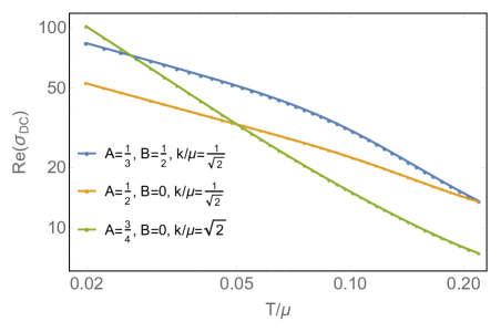
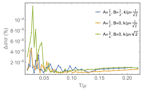
Figure 6: Comparison of the two numerical results for the DC conductivity for three different lattices of the form $\mu(x)/\mu=1+A\,\cos\left(k\,x\right)+B\,\cos\left(2k\,x\right)$. The first is obtained from using the analytic formulae involving black hole horizon data in equation (3.15). The second is obtained from the $\omega\rightarrow 0$ limit of the AC conductivity after fitting to a Drude-peak form. The data is superimposed in the figure on the left and the difference is undetectable to the naked eye. The relative difference is shown in the figure on the right hand and we see agreement at a level better than $10^{-4}\%$.

This fit is carried out for $\omega<<T$; in practise in the region $10^{-4}\lesssim\omega/\mu\lesssim 10^{-2}$ and only for values of $\omega/\mu$ significantly smaller than the maximum in Im$(\sigma)$ (see figure 1). This leads to the results, including a numerical result for the DC conductivity given by $K\tau$, which we summarise in table 1. Comparing this quantity with the result that is obtained from our formulae (3.3) in the last section, we find excellent agreement for both monochromatic and dichromatic lattices; see figure 6. We also note for comparison that the value of $K/\mu$ for the AdS-RN black hole (i.e. with no lattice deformation) is given by $(K/\mu)_{RN}=q^{2}/(\mu(T^{tt}+T^{xx}))$ [1] and hence

$$(K/\mu)_{RN}=\frac{1}{2\sqrt{3+(4\pi T/\mu)^{2}}-4\pi T/\mu}$$ (4.28)

which differs a little from the lattice results.

$T/\mu$	$\tau\mu$	$K/\mu$	$K\tau$	$2<\omega\tau<8$
0.14	53.31	0.33	17.86	$0.036<\omega/\mu<0.15$
0.080	75.99	0.34	25.84	$0.026<\omega/\mu<0.11$
0.039	117.05	0.32	37.53	$0.017<\omega/\mu<0.068$
0.020	175.58	0.30	52.98	$0.011<\omega/\mu<0.046$
0.015	204.66	0.30	60.52	$0.0098<\omega/\mu<0.039$

Table 1: Parameters after fitting to the Drude behaviour (4.27) for small $\omega$, for the monochromatic lattices displayed in figure 1.Note that $K\tau$ gives a numerical estimate for the DC conductivity which can be compared with the analytic result; see figure 6.

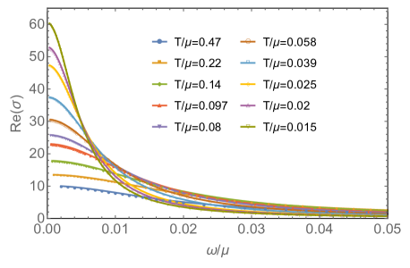
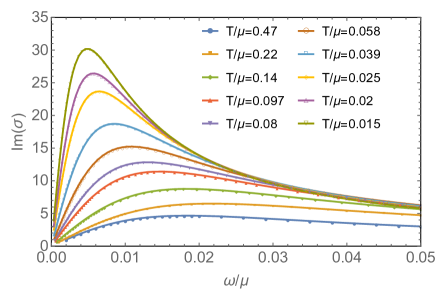
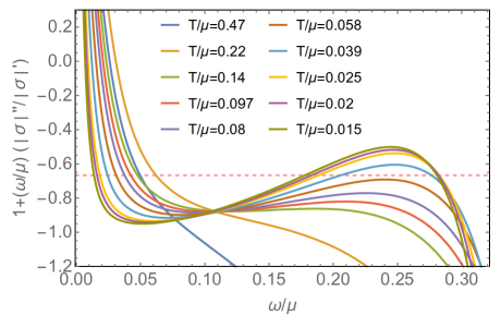
Figure 1: The real (top left) and the imaginary (top right) parts of the optical conductivity $\sigma$ as a function of $\omega/\mu$ for a monochromatic lattice $\mu(x)/\mu=1+A\cos\left(k\,x\right)$, with $A=1/2$, $k/\mu=1/\sqrt{2}$, and various $T/\mu$ close to the origin. The conductivity clearly shows a Drude-like peak developing at low temperatures. The bottom figure shows the corresponding behaviour of $1+(\omega/\mu)\,\left|\sigma\right|^{\prime\prime}/\left|\sigma\right|^{\prime}$ and there is no evidence of a mid-frequency intermediate scaling with exponent $-2/3$. Note the different horizontal scale in the top and bottom figures.

We now make some specific comparisons with the results of [5]. To do so, we need to take into account a relative scaling of the chemical potential: $\mu=\sqrt{2}\mu^{there}$. Then the monochromatic lattices that we have been considering for the specific temperature $T/\mu=0.039$ correspond to those in figures 6-9 of [5]. We find very good agreement with figure 6 which shows the charge density of the background black holes. We find less good agreement (of the order of a couple of percent) with the plot of the AC conductivity in figure 8 of [5]. Furthermore, in figure 9 of [5] distinct kinks are found in the AC conductivity which we do not see for these or in fact any of our lattices. We discuss the issue of intermediate scaling claimed in [5] in the next subsection.

4.3.2 Absence of intermediate scaling

The next feature that we would like to report on is the possibility of an intermediate frequency scaling behaviour of the form

$$|\sigma(\omega)|\sim B\omega^{-2/3}+C\,,$$ (4.29)

where $B,C$ are frequency independent constants. Such a scaling was reported in [4, 5], based on log-log plots, for the approximate range $2<\omega\tau<8$, where $\tau$ is obtained from the fit to the Drude peak. If this scaling is present then a sharp diagnostic is that $1+(\omega/\mu)|\sigma|^{\prime\prime}/|\sigma|^{\prime}\sim-2/3$. As illustrated in figure 1, we find no evidence for such scaling (the relevant range of $\omega/\mu$ is given in table 1). Moreover, we find similar behaviour to what we saw for a homogeneous Q-lattice in [10]. Finally, we highlight that at very low temperatures, where the Drude peak becomes sharper, the function $1+(\omega/\mu)|\sigma|^{\prime\prime}/|\sigma|^{\prime}$ approaches 2 as $\omega\to 0$ and, in addition, there is a scaling region with exponent $-1$, visible in figure 1; both of these features arise from (4.27).

We make a final comparison with [5] for the specific case of $T/\mu=0.039$. In figure 9 of [5] a log-log plot suggested a scaling with exponent $-2/3$ for the approximate range $0.02\lesssim\omega/\mu\lesssim 0.07$. However, there is no evidence for this scaling in the bottom panel in figure 1. In fact, for this range of $\omega/\mu$ we can see from the top panels in figure 1 that we are not too far from the Drude peak. Indeed, we have checked that our fit to the Drude behaviour is in fact rather reasonable over this entire range of $\omega/\mu$.

4.3.3 Scaling behaviour and $AdS_{2}\times\mathbb{R}^{2}$ in the IR as $T\to 0$

We next discuss how the black holes behave as $T\to 0$. When the constant part of $\mu(x)$ is non-vanishing, i.e. $\mu\neq 0$, for the monochromatic lattices we find that in the far IR the solutions all seem to approach $AdS_{2}\times\mathbb{R}^{2}$. More precisely, as we discuss in the next paragraph, we find that the black hole solutions exhibit a low temperature scaling behaviour that are consistent with the $T=0$ solutions interpolating between $AdS_{4}$ in the UV and $AdS_{2}\times\mathbb{R}^{2}$ perturbed by an irrelevant operator in the locally quantum critical theory in the IR. In particular, for the values of $k$ that we have looked at and for the temperatures we have looked at, we find no evidence for the “floppy” ground states discussed in [32]. Some additional comparisons with this work are made in appendix C.

In figure 2 we show the behaviour of the DC conductivities $\sigma$ and $\bar{\kappa}$, obtained from (3.3), as well as their log-derivatives, as a function of temperature for four different monochromatic lattices. At low temperatures we see that the conductivities approach the scaling behaviour given in (3.40) and (3.41) as depicted by the dashed red lines. Note that the low-temperature scaling is obtained by taking the lowest temperature black hole to deduce the approximate value of the renormalised wave-number $\bar{k}$ given in (3.41). The renormalisation factor $\bar{\lambda}$, defined in (3.42) is actually very small: for example it is $\bar{\lambda}=1.027$, for the case $A=1/2$, $k/\mu=1/\sqrt{2}$ (red) and for other cases it is given in table 2. Note the former case has $\bar{\kappa}\to 0$ while for the latter case $\bar{\kappa}\to\infty$ as $T\to 0$. At high temperatures we see that $\sigma\to 1+2/A^{2}=9$ in agreement with (3.4).

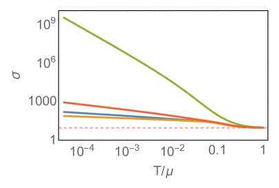
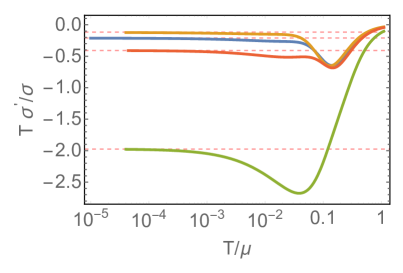
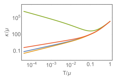
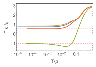
Figure 2: Plots of the DC conductivity for $\sigma$ (top left) and $\bar{\kappa}$ (bottom left), obtained from (3.3), against temperature for four monochromatic lattices of the form $\mu(x)/\mu=1+A\,\cos\left(k\,x\right)$, all with $A=1/2$ and $k/\mu=\sqrt{2}/3$ (orange), $2\sqrt{2}/5$ (blue), $1/\sqrt{2}$ (red) and $\sqrt{2}$ (green). The red dashed lines on the right hand plots indicate the low-temperature scaling behaviour, given in (3.40) expected for black holes approaching $AdS_{2}\times\mathbb{R}^{2}$ in the far IR. The $k/\mu=\sqrt{2}$ case provides an example where $\bar{\kappa}$ diverges as $T\to 0$, while the other cases are examples where $\bar{\kappa}$ vanishes as $T\to 0$. In all cases $\kappa$ vanishes linearly with $T$. As $T\to\infty$ we see that $\sigma\to 1+2/A^{2}=9$, marked with a red dashed line in the top left figure, in agreement with (3.4).

4.3.4 Sum rules on conductivity

It is illuminating to check sum-rules associated with the AC electrical conductivity. As $\omega\to\infty$ we have $\sigma(\omega)\to 1$ and hence after defining the integrated spectral weight as:

$$S(\omega/\mu)\equiv\int_{0}^{\omega/\mu}(Re[\sigma(\omega^{\prime})]-1)d\omega^{\prime}\,,$$ (4.30)

following [34] we might expect that $\lim_{\omega\to\infty}S(\omega)\to 0$. We briefly discuss the proof highlighting the underlying assumptions. In the absence of instabilities the retarded Greens function $G_{J^{x}J^{x}}(\omega)$ is analytic in the upper half plane and we assume this includes the real axis. We also need to assume that for $Im(\omega)>0$ that the function $G_{J^{x}J^{x}}(\omega)-i\omega$ vanishes faster than $1/|\omega|$ as $|\omega|\to\infty$. The Kramers-Krönig relations then imply that $\lim_{\omega\to\infty}S(\omega)=\lim_{\omega\to 0^{+}}\pi/2\text{Re}[G_{J^{x}J^{x}}(\omega)-i\omega]=0$, provided that $\text{Re}[G_{J^{x}J^{x}}(0)]=0$ which is satisfied in our case (see figure 1). This sum rule is manifest in figure 3 for monochromatic lattices.

We also note from figure 3 that as $T\to 0$, the function $S(\omega)$ is developing a step like behaviour near $\omega\to 0$, corresponding to the Drude-peak becoming a delta function exactly at $T=0$. It would appear that the weight of the delta function is slightly smaller than that of the AdS-RN black hole. To see this, and to make an additional comparison, we note that the electrical conductivity of the AdS-RN black hole has a delta function for all temperatures with $\sigma^{RN}(\omega)=1+\sigma_{0}(\omega)+K_{RN}\left(\frac{i}{\omega}+\pi\delta(\omega)\right)$ where $\sigma_{0}(\omega)$ is an analytic function that falls off faster than $1/|\omega|$ at infinity and $K_{RN}$ is given in (4.28). Thus for AdS-RN black holes, as $\omega/\mu\to 0$ we should have $S(\omega/\mu)\to(\pi/2)K_{RN}/\mu$. At $T=0$ we have $K_{RN}/\mu=q/\mu^{2}=1/(2\sqrt{3})$ and hence $S(\omega/\mu)\sim 0.45$ as $\omega/\mu\to 0$, which is slightly bigger than the weight of the delta function appearing at $T=0$ for the lattice black holes. We can also consider lattice black holes at finite temperature with fixed $k/\mu$ and then take the lattice strength $A\to 0$. In this limit we should find that as $\omega\to 0$, $S(\omega/\mu)$ should approach the AdS-RN result at the same temperature; this is also confirmed in figure 3 for the case of $T/\mu=0.12$ for which $(\pi/2)K_{RN}/\mu\sim 0.51$.

We can also consider a different sum rule first discussed in [35]. Defining

$$S_{d}(\omega/\mu)\equiv\int_{0}^{\omega/\mu}(Re[\frac{1}{\sigma(\omega^{\prime})}]-1)d\omega^{\prime}\,,$$ (4.31)

the sum rule is $\lim_{\omega\to\infty}\tilde{S}_{d}(\omega)\to 0$. This arises from the electromagnetic duality of the $D=4$ Einstein-Maxwell theory, with the dual gauge-field being associated with a second CFT arising from an alternative quantisation scheme [42] (for related discussion see also [43, 44, 45, 46].) In our setup the lattice deformation with chemical potential $\mu(x)$ gets mapped to a magnetic field that is spatially modulated in the $x$ direction. We have verified this sum rule as shown in figure 3.

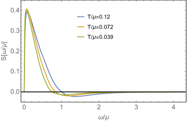
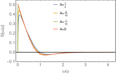
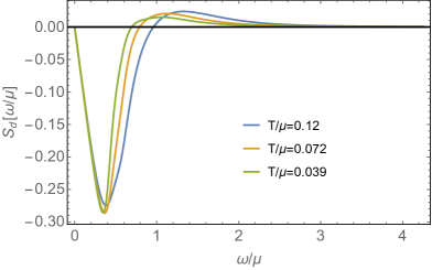
Figure 3: Sum rules for monochromatic lattices. The top left panel plots the integrated spectral weight $S(\omega/\mu)$, defined in (4.30), for a monochromatic lattice $\mu(x)/\mu=1+A\cos\left(k\,x\right)$, with $A=1/2$, $k/\mu=1/\sqrt{2}$ (as in figure 1) for three different temperatures, and we see it vanishes when $\omega/\mu\to\infty$ as expected from the first sum rule. As $T/\mu\to 0$ we see that $S(\omega/\mu)$ is developing a step-like behaviour corresponding to the appearance of a delta function with weight smaller than the $T=0$ AdS-RN black hole (which has the value $\sim 0.45$). The top right panel considers monochromatic lattices with $k/\mu=1/\sqrt{2}$ and fixed $T/\mu=0.12$ and various $A$. As $A\to 0$ we see that the $S(\omega/\mu)$ is developing a step-like behaviour corresponding to the appearance of a delta function with the same weight as the AdS-RN black hole at the same temperature (which for this case has the value $\sim 0.51$). The bottom panel plots $S_{d}(\omega/\mu)$, defined in (4.31), for the same monochromatic lattices as in the top left panel and we see that the second sum rule is also satisfied.

4.3.5 Intermediate resonances

Next, we highlight some interesting features of the optical conductivity that appear at intermediate frequencies, as illustrated in figure 4. In particular for the monochromatic lattices with $k/\mu=1/(3\sqrt{2})$ and various lattice strengths $A$, we find that there is a bump in the optical conductivity just outside the Drude-peak. Now the Drude peak arises because there is a pole near $\omega=0$ in the $T^{tx}T^{tx}$ correlator. One might expect that there could be additional features due to contributions from the sound modes. From the analysis of [37] at $T=0$ we have $v_{s}=1/\sqrt{2}$ and furthermore it was shown that $v_{s}$ has only a weak dependence on temperature in [47]. Thus we might expect to see a resonance appear near $\omega/\mu\sim v_{s}(k/\mu)\sim 1/6$, and this is what is seen in figure 4.

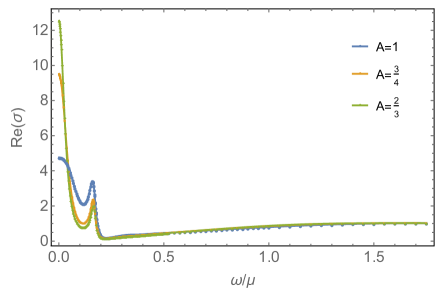
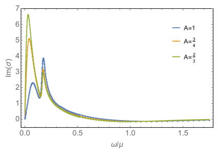
Figure 4: The real (left) and the imaginary (right) parts of the optical conductivity as a function of $\omega$ for various monochromatic lattices $\mu(x)/\mu=1+A\,\cos\left(k\,x\right)$. The three different cases have fixed temperature $T/\mu\approx 0.0795$ and period $k/\mu=\left(3\,\sqrt{2}\right)^{-1}$ but varying lattice strength $A$. We clearly see the appearance of a resonance associated with the sound mode frequency $\omega/\mu\sim v_{s}k/\mu\sim 1/6$.

Note that such resonances are also seen for the lattices with $A=1/2$, $k/\mu=1/\sqrt{2}$ at $\omega/\mu\sim v_{s}k/\mu\sim 1/2$, but these lie outside the range plotted in figure 1.

Similarly, for the dichromatic lattices (4.26), containing wave-numbers $k$ and $2k$, we might expect to see structure in the optical conductivity at frequencies $\omega/\mu\sim v_{s}(k/\mu)$ and also twice this frequency. Such behaviour is illustrated in figure 5.

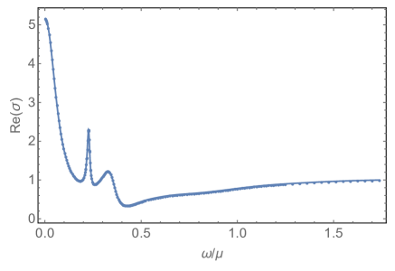
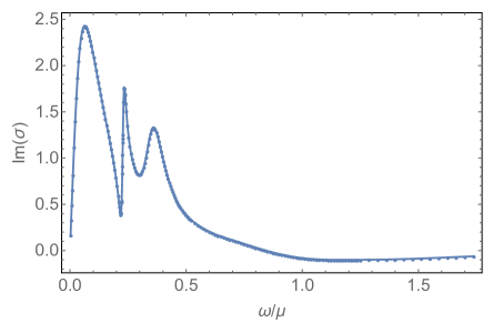
Figure 5: The real (left) and the imaginary (right) parts of the optical conductivity as a function of $\omega/\mu$ for the dichromatic lattice $\mu(x)/\mu=1+A\cos\left(k\,x\right)+B\cos\left(2k\,x\right)$, with $A=1/2$, $B=1$, $k/\mu=1/\left(3\sqrt{2}\right)$ and $T/\mu\approx 0.0796$. In this case we see two resonances associated with sound modes at $\omega/\mu\sim v_{s}k/\mu\sim 1/6$ and also $\omega/\mu\sim v_{s}(2k)/\mu\sim 1/3$.

4.3.6 Conductivities for higher Fourier modes

Until this point we have focussed on the zero-mode of the current $\mathcal{J}$ appearing in (4.22) in order to extract the optical conductivity as in (4.24). We can also extract the higher Fourier modes of $\mathcal{J}$ and construct the corresponding Greens function. If we write the $n$th Fourier mode as $\mathcal{J}_{n}$, then we can define

$$G_{n}=\frac{\mathcal{J}_{n}}{\mu_{J}}\,,$$ (4.32)

which defines the current two point correlator $G_{J_{x}J_{x}}\left(k_{1}=n\,k_{L},k_{2}=0,\omega\right)$. It is worth emphasising that these correlators with $k_{2}\neq k_{1}$ are non-vanishing as a consequence of the broken translation invariance of the backgrounds. For the monochromatic lattice of figure 1, with $A=1/2$, $k=1/\sqrt{2}$ and $T/\mu=0.08$, in figure 7 we have plotted the real and imaginary parts of $G_{n}/\omega$ for $n=1,2$ and $3$. Notice that the conservation of the current $\partial_{a}\mathcal{J}^{a}=0$ implies that at $\omega=0$ we have $\mathcal{J}_{n}=0$ if $n\neq 0$, as we see in the plot. Observe that there is a peak in the imaginary part at $\omega/\mu\sim 0.5$, which is associated with the sound mode at $\omega/\mu\sim v_{s}k/\mu\sim 1/2$.

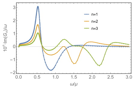
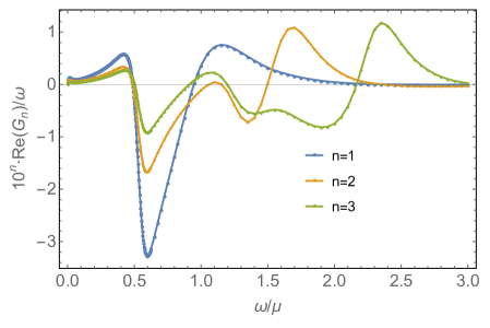
Figure 7: A plot of the imaginary (left) and real (right) parts of $G_{n}/\omega$, where $G_{n}$ is the Green’s function for the $n$th Fourier modes of the current as in (4.32). The plots are for the monochromatic lattice in figure 1 with $T/\mu=0.08$ and for Fourier modes $n=1,2$ and $3$. Notice that different vertical scales are used for each $n$. Observe they all vanish at $\omega=0$, as expected from current conservation, and the feature at $\omega/\mu\sim v_{s}k/\mu\sim 1/2$, associated with the sound mode.

4.3.7 A dirty lattice

We have also constructed black holes for “dirty lattices”, comprising of many wave-numbers and random phases, with a view to modelling disorder (see e.g. [48, 49, 50, 51, 52, 53, 54].) Specifically, we consider a truncated version of Gaussian white noise given by

$$\mu(x)=1+\frac{A}{\sqrt{n_{m}}}\,\sum_{n=1}^{n_{m}}\,\cos(n\,k\,x+\theta_{n})\,,$$ (4.33)

for a random collection of phases $\theta_{n}$ sampled over a uniform distribution. The maximum wavenumber, $n_{m}\,k$, represents a UV cutoff while the overall period, $2\pi/k$, is the IR cutoff. A specific example that we analysed has $A=1/2$, $k/\mu=1/(4/\sqrt{2})$, $T/\mu=0.08$ and $n_{max}=10$, with the corresponding local chemical potential plotted in figure 8. In figure 8 we also show the optical conductivity: it is manifest that these lattices continue to exhibit a Drude-peak with a DC electrical conductivity that is in precise agreement with our analytic result. We also expect resonances at mid-frequencies arising from sound modes, and we have verified the existence of the first peak at $\omega/\mu\sim v_{s}k/\mu\sim 0.125$, as well as the next two at roughly twice and three times this value.

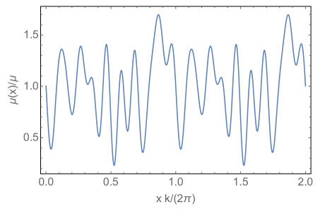
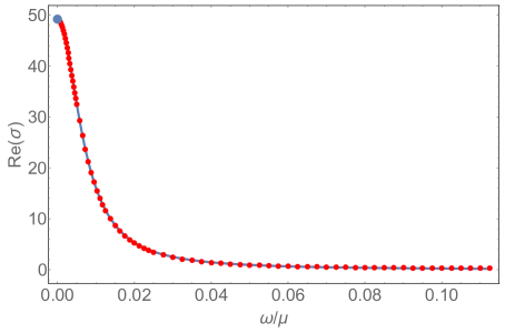
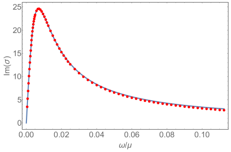
Figure 8: The top panel shows the chemical potential for a “dirty lattice” constructed from ten different wave numbers as in (4.33) with $A=1/2$ and $k/\mu=1/(4/\sqrt{2})$. In the bottom panels we show the real (bottom left) and imaginary (bottom right) parts of the optical conductivity for this lattice at $T/\mu=0.08$. The real part exhibits a Drude peak with a DC conductivity that agrees precisely with the analytic result obtained from the black hole horizon, indicated by a blue dot.

5 Final Comments

We have found a remarkably compact analytic expression for the thermoelectric DC conductivity for a class of inhomogeneous black hole lattices, for all temperatures, generalising the results for homogeneous lattices in [12, 14]. Our results provide strong evidence that this approach can be generalised to arbitrary lattices. It would be interesting to next examine an inhomogeneous lattice with a UV deformation that depends on more than one spatial dimension, as in the recent construction of holographic checkerboards in [55].

Our results provide a powerful way to obtain the low-temperature scaling behaviour of the DC conductivity. For translationally invariant ground states, such as black hole solutions which approach irrelevant deformations of $AdS_{2}\times\mathbb{R}^{2}$ in the far IR, when the lattice strength is small one can also use the memory matrix formalism [31], and in this case we find precise agreement. On the other hand, if one approaches a ground state which breaks translations, as in [12, 20], then the memory matrix formalism cannot be used and so our analytic results provide a particularly powerful tool to study the properties of these novel holographic ground states.

Here and in [14], we have seen that as $T\to\infty$ the UV lattice deformation leads to a modification of the DC conductivity away from the value of the optical conductivity $\sigma(\omega)$ in the limit $\omega\to\infty$. In this paper, we have seen that a periodic chemical potential $\mu(x)$ leads to a saturation of the electric DC conductivity to a constant value as $T\to\infty$, with the value depending on $\mu(x)$ as in (3.4). This is a kind of generalised Mott-Ioffe-Regel bound [27, 28] without quasi-particles. It is also worth noting that as $T\to\infty$ we find that the optical conductivity approaches unity for all values of $\omega/\mu$, except at $\omega/\mu\to 0$ where it jumps to the higher DC value.

We have also made detailed constructions of the inhomogeneous black holes arising in Einstein-Maxwell theory for various periodic chemical potentials. We focussed in most detail on monochromatic lattices, associated with a single wave-number, $k$, but we also considered dichromatic lattices, with wave-numbers $k$ and $2k$ and the same phase. In addition we constructed black holes that model a dirty lattice which were built from ten sequential wave-numbers with random phases. The black holes, as well as the optical conductivity were obtained by numerically solving PDEs. We have found Drude peaks in the optical conductivity at finite temperature, as in [4], but, in contrast to [4], we do not find any intermediate scaling for the monochromatic lattices. At low temperatures our ground states for the monochromatic lattices all seem to approach $AdS_{2}\times\mathbb{R}^{2}$ in the far IR and, specifically, we find the DC scaling behaviour is precisely consistent with this. While it is possible that lowering the temperature of the black holes further will reveal some exotic new ground states, as in [32], we feel this is unlikely. It would be interesting to know if exotic ground states appear for stronger lattice deformations and/or for other deformations of the chemical potential.

We have shown that the monochromatic, dichromatic and dirty lattices naturally give rise to mid frequency resonances that can be associated with sound modes. It will be interesting to consider this issue in more detail for the dirty lattices since in the limit where the number of modes and the characteristic wave-number is going to zero (i.e. $n_{m}\to\infty$, $k\to 0$ in (4.33)) the resonances may coalesce and change the analytic structure of the Greens functions in the mid-frequency region.

Appendix A The stress tensor and heat current

For the perturbed black holes of interest we can obtain the heat current from the stress tensor following the approach of [14]. From [56] we can write the stress tensor and the current as

$$\frac{1}{2}\tilde{T}^{\mu\nu} =-K^{\mu\nu}+K\gamma^{\mu\nu}-2\gamma^{\mu\nu}+G^{\mu\nu}\,,$$

$$\tilde{J}^{\nu} =-n_{\mu}F^{\mu\nu}\,,$$ (A.1)

where $n^{\mu}$ is the unit normal to the boundary, $K_{\mu\nu}=(\delta_{\mu}{}^{\rho}+n_{\mu}n^{\rho})\nabla_{\rho}n_{\nu}$, $G^{\mu\nu}$ is the Einstein tensor of the boundary metric $\gamma$ and expressions are to be evaluated at the boundary $r\to\infty$.

For all of the black holes that we considered in calculating the DC conductivities, including the perturbation, we have

$$n_{\mu}=\left(\frac{H_{rr}}{U}\right)^{1/2}(1+\frac{U\delta g_{rr}}{2H_{rr}})\,(0,1,0,0)\,.$$ (A.2)

For the black hole backgrounds (with vanishing perturbation) we obtain the following expressions

$$\tilde{T}^{tt} =\frac{1}{UH_{tt}}\Bigg{[}4-\frac{U^{1/2}}{H_{rr}^{1/2}}\partial_{r}\ln\Sigma\Bigg{]}+2G^{tt}\,,$$

$$\tilde{T}^{xx} =\frac{1}{e^{B}\Sigma H_{tt}(UH_{rr})^{1/2}}\Bigg{[}\partial_{r}(UH_{tt})-UH_{tt}\left(\partial_{r}\ln\frac{e^{B}}{\Sigma}+4\frac{H_{rr}^{1/2}}{U^{1/2}}\right)\Bigg{]}$$

$$\qquad\qquad\qquad-\frac{1}{2\Sigma^{2}H_{tt}e^{2B}}\left(\partial_{x}\ln\frac{e^{B}}{\Sigma}\right)\left(\partial_{x}H_{tt}\right)\,,$$

$$\tilde{T}^{yy} =\frac{e^{B}}{\Sigma H_{tt}(UH_{rr})^{1/2}}\Bigg{[}\partial_{r}(UH_{tt})-UH_{tt}\left(\partial_{r}\ln\frac{e^{-B}}{\Sigma}+4\frac{H_{rr}^{1/2}}{U^{1/2}}\right)\Bigg{]}+2G^{yy}\,,$$

$$\tilde{J}^{t} =\frac{1}{(UH_{rr})^{1/2}H_{tt}}\partial_{r}a_{t}\,,$$ (A.3)

where we have omitted the explicit expressions for $G^{tt}$ and $G^{yy}$ for brevity. As $r\to\infty$ we have $\tilde{T}^{ab}\sim r^{-5}$ and $\tilde{J}^{a}\sim r^{-3}$ so it is convenient to define

$$T^{ab}=r^{5}\tilde{T}^{ab}\,,\qquad J^{a}=r^{3}\tilde{J}^{a}\,.$$ (A.4)

We next consider the perturbation about the black holes backgrounds discussed in section 3, but with a general time dependence in $\delta g_{tx}$ for the moment, finding

$$\tilde{T}^{tx}= \frac{1}{e^{B}\Sigma H_{tt}(UH_{rr})^{1/2}}\Bigg{[}-\delta g_{tx}(t,r,x)\left(\partial_{r}\frac{\ln e^{B}}{\Sigma}+\frac{H_{rr}^{1/2}}{U^{1/2}}\right)$$

$$+\partial_{r}\delta g_{tx}(t,r,x)-H_{tt}\partial_{x}\frac{\delta g_{tr}}{H_{t}t}\Bigg{]}-\frac{\delta g_{tx}(t,r,x)}{2e^{2B}\Sigma^{2}H_{tt}^{2}U}\left(\partial_{x}\frac{\ln e^{B}}{\Sigma}\right)\left(\partial_{x}H_{tt}\right)\,,$$ (A.5)

where we have included the argument of $\delta g_{tx}$, here and below, for clarity. It will be convenient, shortly, to note that

$$U^{1/2}H_{tt}^{1/2}\Sigma\left(UH_{tt}\tilde{T}^{tx}-\delta g_{tx}(t,r,x)\tilde{T}^{xx}\right)=\frac{U^{2}H_{tt}^{3/2}}{e^{B}H_{rr}^{1/2}}\Bigg{[}\partial_{r}\left(\frac{\delta g_{tx}(t,r,x)}{UH_{tt}}\right)-\partial_{x}\frac{\delta g_{tr}}{UH_{tt}}\Bigg{]}\,.$$ (A.6)

We now consider the particular linearised time-dependence for the perturbation given in sections 3.2 and 3.3:

$$\delta A =-tEdx+t\zeta a_{t}+{\delta a_{\mu}}(r,x)dx^{\mu}\,,$$

$$\delta ds^{2} =-2t\zeta UH_{tt}dtdx+\delta g_{\mu\nu}(r,x)dx^{\mu}dx^{\nu}\,,$$ (A.7)

with falloffs of ${\delta a_{\mu}}(r,x)$ and $\delta g_{\mu\nu}(r,x)$ as $r\to\infty$ chosen so that the only sources are parametrised by $E$ and $\zeta$. Now these time-dependent sources give rise to a time-independent expression for $\tilde{J}^{x}$:

$$\tilde{J}^{x}=\frac{e^{-B}}{\sqrt{H_{rr}H_{tt}}}\,\left[\delta g_{tr}\partial_{x}a_{t}-\delta g_{tx}(r,x)\partial_{r}a_{t}+H_{tt}U\left(\partial_{x}\delta a_{r}-\partial_{r}\delta a_{x}\right)\right]\,,$$ (A.8)

which, when evaluated at $r\to\infty$ and using (A.4), agrees with the expression for $J$ in (3.3). By contrast we obtain a time-dependent component in $T^{tx}$. Explicitly, from (A) we immediately obtain

$$\tilde{T}^{tx} =\frac{1}{e^{B}\Sigma H_{tt}(UH_{rr})^{1/2}}\Bigg{[}-\delta g_{tx}(r,x)\left(\partial_{r}\frac{\ln e^{B}}{\Sigma}+\frac{H_{rr}^{1/2}}{U^{1/2}}\right)$$

$$+\partial_{r}\delta g_{tx}(r,x)-H_{tt}\partial_{x}\frac{\delta g_{tr}}{H_{tt}}\Bigg{]}-\frac{\delta g_{tx}(r,x)}{2e^{2B}\Sigma^{2}H_{tt}^{2}U}\left(\partial_{x}\frac{\ln e^{B}}{\Sigma}\right)\left(\partial_{x}H_{tt}\right)-\zeta t\tilde{T}^{xx}\,,$$

$$\equiv\tilde{T}^{tx}_{0}-\zeta t\tilde{T}^{xx}\,.$$ (A.9)

Returning now to (A.6) and substituting in (A) we find that all of the time dependence drops out and hence we can conclude that

$$U^{1/2}H_{tt}^{1/2}\Sigma\left(UH_{tt}\tilde{T}^{tx}_{0}-\delta g_{tx}(r,x)\tilde{T}^{xx}\right)=\frac{U^{2}H_{tt}^{3/2}}{e^{B}H_{rr}^{1/2}}\Bigg{[}\partial_{r}\left(\frac{\delta g_{tx}(r,x)}{UH_{tt}}\right)-\partial_{x}\frac{\delta g_{tr}}{UH_{tt}}\Bigg{]}\,.$$ (A.10)

Evaluating both sides at $r\to\infty$ we deduce that

$$r^{5}\tilde{T}^{tx}_{0}=\lim_{r\to\infty}\frac{U^{2}H_{tt}^{3/2}}{e^{B}H_{rr}^{1/2}}\Bigg{[}\partial_{r}\left(\frac{\delta g_{tx}(r,x)}{UH_{tt}}\right)-\partial_{x}\frac{\delta g_{tr}}{UH_{tt}}\Bigg{]}\,.$$ (A.11)

Recalling the expression for $Q$ given in (3.1), we deduce that

$$T^{tx}-\mu J^{x}=Q-\zeta tT^{xx}\,.$$ (A.12)

Now as explained in appendix C of [14], the time dependent piece is associated with a static susceptibility for the $Q$ $Q$ correlator, which we see is explicitly given by $T^{xx}$ of the background black holes. On the other hand the time independent piece is associated with the DC conductivity.

Appendix B Convergence tests

In this section we will provide a few details on three different convergence tests that we carried out for the numerical methods which we discussed in sections 4.1 and 4.2.

For the black hole backgrounds, in the continuum limit, which is approached as the number of grid points is taken to infinity, we expect that the norm of the DeTurck vector, $\xi^{2}$, should approach zero uniformly everywhere on our computational grid. Checking that this happens is the first test that we performed. Along the same lines, our backgrounds should satisfy the equations of motion (2) without the additional DeTurck term. Correspondingly, our second convergence test is to check the absolute value of the trace of Einstein’s equations in (2).

Our third check concerns the convergence properties of the perturbation about the background black holes in order to extract the optical conductivity as described in section 4.2. As we pointed out in the main text, the six functions that we used in the perturbation ansatz (4.2) should solve ten equations of motion, of which four are constraints that we impose on the black hole horizon. As a non-trivial check of our numerics, we check that the constraints are satisfied everywhere in the bulk in the continuum limit. As an illustration of this we can take the trace of Einstein’s equations, expand it to first order in the perturbation and then examine the absolute value of the leading term.

Let us present some results of these tests for the specific monochromatic lattice $\mu(x)=\mu\,\left(1+\frac{1}{2}\,\cos\left(\frac{\mu}{\sqrt{2}}\,x\right)\right)$ for three different temperatures $T/\mu\approx 0.035$, $T/\mu\approx 0.02$ and $T/\mu\approx 0.015$. These black holes have been discussed in the main text and some of their properties are presented in figure 1. In order to give a more detailed treatment, we divide our computational grid into two halves: the “boundary” half, defined by $0<z<1/2$, and the “horizon” half, defined by $1/2<z<1$. In all of our tests we have fixed the number of points in the periodic, field theory direction to be $N_{x}=45$ and then we vary the number of points, $N$, in the radial direction. For the perturbation convergence tests we have fixed the frequency $\omega/\mu\approx 0.0008$ which for the three temperatures is very close to the top of the Drude peak; we do this because it is a region in $\omega/\mu$ which is challenging numerically.

In figure 9 we show the results of the two convergence tests for the black hole solutions, discussed above, for the boundary and horizon regions. The boundary expansion (4.1) suggests that we should have convergence not better than fifth order for the boundary region and indeed we find that while $\xi_{b}^{2}$ converges as $N^{-8}$, the trace of Einstein’s equations converges as $N^{-4.6}$. On the other hand, close to the horizon, we have an analytic expansion and we find convergence of the same quantities of the form $N^{-11.7}$ and $N^{-5.7}$, respectively.

In figure 10 we show a plot of the convergence test for the perturbation that we discussed above. For the range of resolutions shown in the figure we find a convergence rate scaling like $N^{-5.4}$ which is suggestive that all the error comes from the horizon and, moreover, from the fact that our background satisfies the DeTurck modified equations instead of Einstein’s.

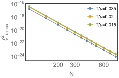
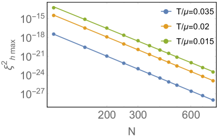
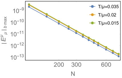
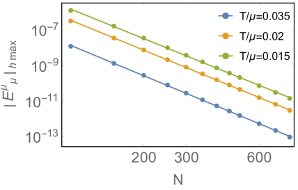
Figure 9: Convergence tests for the numerical construction of monochromatic lattice black holes of figure 1 for three different temperatures. The figures on the left denote convergence tests in the boundary region, while those on the right correspond to the horizon region. We have plotted the norm of the de Truck vector, $\xi^{2}$ and the absolute value of the trace of Einstein’s equations $E^{\mu}{}_{\mu}$ against the number of radial points in the grid, $N$, with a fixed number $N_{x}=45$ points in the periodic spatial $x$-direction.

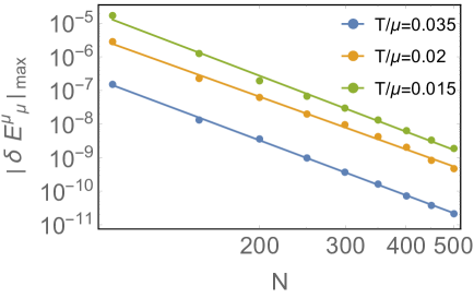
Figure 10: Convergence tests for the numerical construction of the perturbation about the black holes considered in figure 9 that is needed to obtain the AC conductivity. We have plotted $\delta E^{\mu}{}_{\mu}$, which is obtained by considering the trace of Einstein’s equations, expanding it to first order in the perturbation and then taking the absolute value of the leading term, against the number of radial points in the grid, $N$. Again, $N_{x}=45$.

The numerical schemes outlined in section 4 were implemented in C++. The facility of class templates has been particularly helpful to accommodate the various numerical precisions we have used at low temperatures and in the convergence tests. At certain key points of our code we have specialised our templates to double, long double, Intel’s _QUAD and MPFR [57] data types. In particular this was necessary for the relevant sparse linear solver that we used both in Newton’s method and for the linear perturbations for the optical conductivity. For our double precision numerics we have chosen UMFPACK from the SuiteSparse library [58] compiled with Intel’s MKL BLAS which takes advantage of multicore systems when combined with OpenMP. For the three remaining data types we have chosen to use the SparseLU solver from the Eigen3 template library [59]. In writing our code we have greatly benefited from the float128 wrapper class of the Boost C++ library [60].

Concerning the plots appearing in figures 9 and 10, we have found that double precision is saturated when we reach 450 points in the radial direction after which we need to use long double precision numerics for the backgrounds. As far as the conductivity perturbation is concerned, we found that _QUAD precision had to be used when we reach 300 points in the radial direction. For these cases the corresponding black hole background was computed using the same _QUAD precision.

Appendix C Further comments on scaling behaviour

The black holes that we have constructed numerically, described in section 4, are consistent with the $T=0$ limits approaching domain wall solutions interpolating from $AdS_{2}\times\mathbb{R}^{2}$ in the IR to $AdS_{4}$ in the UV. This can be contrasted with the conclusion of [32] where it was argued that the $T=0$ ground states have an inhomogeneous IR behaviour. Here we would like to provide a possible explanation for the disparity.

As illustrated in figure 2 we have seen that for temperatures as low as $T/\mu\sim 4\times 10^{-5}$, and $T/\mu\sim 9.8\times 10^{-6}$ for one specific case, the electrical and thermal DC conductivities exhibit a clear scaling behaviour, exactly consistent with (3.40) and (3.41), predicted from the dimension of the least irrelevant operator about $AdS_{2}\times\mathbb{R}^{2}$. It is also illuminating to consider a quantity $\varpi$ introduced in [32]. Let $\mathcal{W}=||\partial_{y}||^{2}_{r=r_{+}}$ and then, by considering the variation along the $x$ direction, define

$$\varpi=\frac{\mathcal{W}_{max}}{\mathcal{W}_{min}}-1\,.$$ (C.1)

If the $T=0$ ground states have $AdS_{2}\times\mathbb{R}^{2}$ in the IR, then this should approach $0$ at $T=0$. More precisely, it should approach $0$ with a specific scaling behaviour which can be extracted from the analysis of [31, 37]:

$$\varpi\sim T^{\Delta(\bar{k})-1}\,.$$ (C.2)

It is worth restating here that $\bar{k}$ is related to the UV lattice factor as in (3.42), which involves a renormalisation scale $\bar{\lambda}$ that depends on the UV data. In figure 11, for four monochromatic lattices with $A=1/2$ and $k/\mu=\sqrt{2}/3,2\sqrt{2}/5,1/\sqrt{2}$ and $\sqrt{2}$, we see that $\varpi$ scales exactly as expected for an $AdS_{2}\times\mathbb{R}^{2}$ ground state. Now, a simple but key observation is that if the scaling exponent is small, then the value of $\varpi$ can still be parametrically large, compared to the temperature scale, even when one is in the scaling regime as we see in figure 11 and also in table 2. This situation occurs when $\bar{k}$ is small which arises, in practise when $k$ is small.

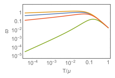
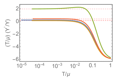
Figure 11: The behaviour of $\varpi$, defined in (C.1), and $\Upsilon$, defined in (C.3), with temperature for monochromatic lattices with $A=1/2$ and $k=\sqrt{2}/3$ (orange)), $k=2\sqrt{2}/5$ (blue), $1/\sqrt{2}$ (red) and $\sqrt{2}$ (green). The red dashed lines on the right hand plots indicate the low-temperature scaling behaviour, given in (C.4) expected for black holes approaching $AdS_{2}\times\mathbb{R}^{2}$ in the far IR. The left plot shows that in the scaling regime, the value of $\varpi$, can be parametrically larger than the scale set by the temperature if the scaling exponent is suitably small. This situation arises for small lattice wave-numbers $k$.

Recalling (3.29), another quantity we can consider is

$$\Upsilon=\int\frac{1}{\Sigma^{(0)}}\left[\partial_{x}\ln{\frac{e^{B^{(0)}}}{\Sigma^{(0)}}}\right]^{2}\,.$$ (C.3)

If the black holes approach $AdS_{2}\times\mathbb{R}^{2}$ in the far IR as $T\to 0$, then we should also have

$$\Upsilon\sim T^{2\Delta(\bar{k})-2}\,.$$ (C.4)

In fact we find that this quantity approaches the scaling behaviour slightly quicker than $\varpi$ and we have illustrated this in figure 11.

For these constructions, in order to keep the error small at low temperatures we used three patches in combination with long double precision. As an indicative example, in lowest temperature black hole for the case $k/\mu=\frac{2\sqrt{2}}{{5}}$ of table 2 we partitioned the coordinate $z$ interval $\left(0,\,1\right)$ into three patches as $\left(0,\,\frac{94}{100}\right]\cup\left[\frac{94}{100},\,\frac{997}{1000}\right]\cup\left[\frac{997}{1000},\,1\right)$. Following the discussion preceding equation (4.12), we took $N_{z}^{1}=1200$, $N_{z}^{2}=2500$ and $N_{z}^{3}=1500$ points in the corresponding intervals while for the $x$ direction we took $N_{x}=45$ points. We used sixth order finite differences in the radial direction while Fourier basis differentiation in the $x$ direction. The resulting geometry turned out to have a maximum $\xi^{2}\sim 10^{-20}$, where $\xi^{2}$ is the norm of DeTurck vector.

$k/\mu$	$T/\mu$	$\varpi$	$s/(8\pi\mu^{2})$	$\bar{\lambda}$	$\Upsilon$
$\frac{\sqrt{2}}{{3}}$	$4.0\times 10^{-5}$	0.964	0.0458	1.04	0.14
$\frac{2\sqrt{2}}{{5}}$	$9.8\times 10^{-6}$	0.396	0.0452	1.03	0.049
$\frac{1}{\sqrt{2}}$	$4.4\times 10^{-5}$	0.140	0.0445	1.03	0.012
$\sqrt{2}$	$4.0\times 10^{-5}$	$3.12\times 10^{-5}$	0.0425	1.01	2.9$\times 10^{-9}$

Table 2: The values of $\varpi$ (see (C.1), entropy density $s$, renormalisation of length scale $\bar{\lambda}$ (see (3.42)) and $\Upsilon$ (see (C.3)) for the three monochromatic lattices plotted in figure 11, for the given temperature.

To further illustrate our results we can consider the quantity

$$\Delta F^{2}\equiv F^{2}-F^{2}_{RN}$$ (C.5)

where $F^{2}=F_{\mu\nu}F^{\mu\nu}$ is the norm of the field strength for the lattice black holes and $F^{2}_{RN}$ is the corresponding quantity for the AdS-RN black hole at the same temperature. If the black holes are approaching $AdS_{2}\times\mathbb{R}^{2}$ at $T=0$ then this quantity should approach zero at the black hole horizon. It will also vanish at the $AdS_{4}$ boundary, since each term does separately. For the monochromatic lattice with $A=1/2$, $k/\mu=2\sqrt{2}/5$ (as in figure 11) at the lowest temperature $T/\mu=9.8\times 10^{-6}$ we have plotted $\Delta F^{2}$ against the spatial coordinate $x$ and the radial coordinate $z$ in figure 12. The behaviour is consistent with the $T=0$ limit approaching zero at the black hole horizon at $z=1$ followed by a sharp rise to non-trivial behaviour in the bulk, fading to zero at the $AdS_{4}$ boundary at $z=0$. The cyan lines in figure 12 are the location of the boundaries of the patches we discussed in the previous paragraph.

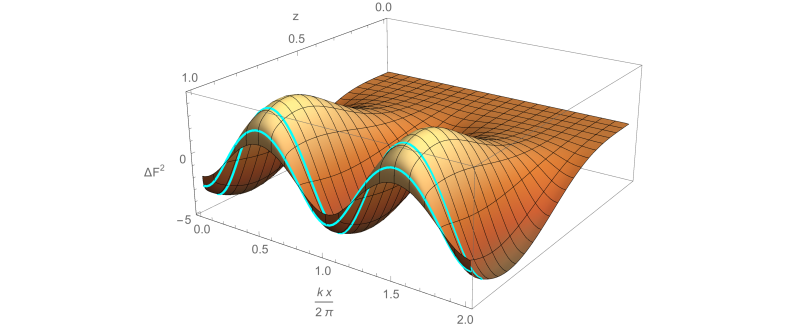
Figure 12: The behaviour of $\Delta F^{2}$ (see (C.5)) for the monochromatic lattice with $k/\mu=2\sqrt{2}/5$ at $T/\mu=9.8\times 10^{-6}$. The behaviour is consistent with it vanishing at $T=0$ at the black hole horizon at $z=1$, consistent with the appearance of $AdS_{2}\times\mathbb{R}^{2}$ in the IR.

We believe our numerical results at finite temperature provide strong evidence that the scaling should continue all the way down to $T=0$ and that the $T=0$ solutions will approach $AdS_{2}\times\mathbb{R}^{2}$ in the IR. We therefore think it is unlikely that the $T=0$ numerical solutions found in [32] are in fact $T=0$ solutions, since, if they were, it would imply that there is a sudden discontinuous jump in the behaviour of the solutions. One possibility is that they are, instead, solutions at very small temperatures and the observed non-vanishing $\varpi$ for small lattice wave-number that was observed in [32] would just correspond to scaling with a small exponent as we have seen for our finite temperature solutions.

References

- [1] S. A. Hartnoll, P. K. Kovtun, M. Muller, and S. Sachdev, “Theory of the Nernst effect near quantum phase transitions in condensed matter, and in dyonic black holes,” Phys. Rev. B76 (2007) 144502, arXiv:0706.3215 [cond-mat.str-el].
- [2] S. A. Hartnoll, “Lectures on holographic methods for condensed matter physics,” Class.Quant.Grav. 26 (2009) 224002, arXiv:0903.3246 [hep-th].
- [3] C. P. Herzog, “Lectures on Holographic Superfluidity and Superconductivity,” J.Phys. A42 (2009) 343001, arXiv:0904.1975 [hep-th].
- [4] G. T. Horowitz, J. E. Santos, and D. Tong, “Optical Conductivity with Holographic Lattices,” JHEP 1207 (2012) 168, arXiv:1204.0519 [hep-th].
- [5] G. T. Horowitz, J. E. Santos, and D. Tong, “Further Evidence for Lattice-Induced Scaling,” JHEP 1211 (2012) 102, arXiv:1209.1098 [hep-th].
- [6] G. T. Horowitz and J. E. Santos, “General Relativity and the Cuprates,” arXiv:1302.6586 [hep-th].
- [7] A. Donos and S. A. Hartnoll, “Interaction-driven localization in holography,” Nature Phys. 9 (2013) 649–655, arXiv:1212.2998.
- [8] Y. Ling, C. Niu, J.-P. Wu, and Z.-Y. Xian, “Holographic Lattice in Einstein-Maxwell-Dilaton Gravity,” JHEP 1311 (2013) 006, arXiv:1309.4580 [hep-th].
- [9] P. Chesler, A. Lucas, and S. Sachdev, “Conformal field theories in a periodic potential: results from holography and field theory,” Phys.Rev. D89 (2014) 026005, arXiv:1308.0329 [hep-th].
- [10] A. Donos and J. P. Gauntlett, “Holographic Q-lattices,” JHEP 1404 (2014) 040, arXiv:1311.3292 [hep-th].
- [11] T. Andrade and B. Withers, “A simple holographic model of momentum relaxation,” JHEP 1405 (2014) 101, arXiv:1311.5157 [hep-th].
- [12] A. Donos and J. P. Gauntlett, “Novel metals and insulators from holography,” JHEP 1406 (2014) 007, arXiv:1401.5077 [hep-th].
- [13] K. Balasubramanian and C. P. Herzog, “Losing Forward Momentum Holographically,” Class.Quant.Grav. 31 (2014) 125010, arXiv:1312.4953 [hep-th].
- [14] A. Donos and J. P. Gauntlett, “Thermoelectric DC conductivities from black hole horizons,” arXiv:1406.4742 [hep-th].
- [15] N. Iqbal and H. Liu, “Universality of the hydrodynamic limit in AdS/CFT and the membrane paradigm,” Phys.Rev. D79 (2009) 025023, arXiv:0809.3808 [hep-th].
- [16] R. A. Davison, “Momentum relaxation in holographic massive gravity,” Phys.Rev. D88 (2013) 086003, arXiv:1306.5792 [hep-th].
- [17] M. Blake and D. Tong, “Universal Resistivity from Holographic Massive Gravity,” Phys.Rev. D88 (2013) 106004, arXiv:1308.4970 [hep-th].
- [18] M. Blake, D. Tong, and D. Vegh, “Holographic Lattices Give the Graviton a Mass,” Phys.Rev.Lett. 112 (2014) 071602, arXiv:1310.3832 [hep-th].
- [19] R. A. Davison, K. Schalm, and J. Zaanen, “Holographic duality and the resistivity of strange metals,” Phys.Rev. B89 (2014) 245116, arXiv:1311.2451 [hep-th].
- [20] B. Goutéraux, “Charge transport in holography with momentum dissipation,” JHEP 1404 (2014) 181, arXiv:1401.5436 [hep-th].
- [21] E. Mefford and G. T. Horowitz, “Simple holographic insulator,” Phys.Rev. D90 no. 8, (2014) 084042, arXiv:1406.4188 [hep-th].
- [22] M. Taylor and W. Woodhead, “Inhomogeneity simplified,” arXiv:1406.4870 [hep-th].
- [23] M. Blake and A. Donos, “Quantum Critical Transport and the Hall Angle,” arXiv:1406.1659 [hep-th].
- [24] A. Donos, B. Gout raux, and E. Kiritsis, “Holographic Metals and Insulators with Helical Symmetry,” JHEP 1409 (2014) 038, arXiv:1406.6351 [hep-th].
- [25] A. Amoretti, A. Braggio, N. Maggiore, N. Magnoli, and D. Musso, “Analytic DC thermo-electric conductivities in holography with massive gravitons,” arXiv:1407.0306 [hep-th].
- [26] T. M. Tritt and M. A. Subramanian, “Thermoelectric materials, phenomena, and applications: A bird’s eye view,” MRS Bulletin 31 (3, 2006) 188–198. http://journals.cambridge.org/article_S088376940000991X.
- [27] O. Gunnarsson, M. Calandra, and J. Han, “Colloquium: Saturation of electrical resistivity,” Rev.Mod.Phys. 75 (2003) 1085–1099, arXiv:cond-mat/0305412 [cond-mat.str-el].
- [28] N. E. Hussey, K. Takenaka, and H. Takagi, “Universality of the Mott-Ioffe-Regel limit in metals,” Phil. Mag. 84 (2004) 2847–2864, arXiv:cond-mat/0404263 [cond-mat.str-el].
- [29] D. v. d. Marel, H. J. A. Molegraaf, J. Zaanen, Z. Nussinov, F. Carbone, A. Damascelli, H. Eisaki, M. Greven, P. H. Kes, and M. Li, “Quantum critical behaviour in a high-Tc superconductor,” Nature 425 (Sept., 2003) 271–274, arXiv:cond-mat/0309172.
- [30] D. van der Marel, F. Carbone, A. B. Kuzmenko, and E. Giannini, “Scaling properties of the optical conductivity of Bi-based cuprates,” Annals of Physics 321 (July, 2006) 1716–1729, arXiv:cond-mat/0604037.
- [31] S. A. Hartnoll and D. M. Hofman, “Locally Critical Resistivities from Umklapp Scattering,” Phys.Rev.Lett. 108 (2012) 241601, arXiv:1201.3917 [hep-th].
- [32] S. A. Hartnoll and J. E. Santos, “Cold planar horizons are floppy,” arXiv:1403.4612 [hep-th].
- [33] M. Headrick, S. Kitchen, and T. Wiseman, “A New approach to static numerical relativity, and its application to Kaluza-Klein black holes,” Class.Quant.Grav. 27 (2010) 035002, arXiv:0905.1822 [gr-qc].
- [34] D. R. Gulotta, C. P. Herzog, and M. Kaminski, “Sum Rules from an Extra Dimension,” JHEP 1101 (2011) 148, arXiv:1010.4806 [hep-th].
- [35] W. Witczak-Krempa and S. Sachdev, “The quasi-normal modes of quantum criticality,” Phys.Rev. B86 (2012) 235115, arXiv:1210.4166 [cond-mat.str-el].
- [36] J. P. Gauntlett and O. Varela, “Consistent Kaluza-Klein Reductions for General Supersymmetric AdS Solutions,” Phys. Rev. D76 (2007) 126007, arXiv:0707.2315 [hep-th].
- [37] M. Edalati, J. I. Jottar, and R. G. Leigh, “Holography and the sound of criticality,” JHEP 1010 (2010) 058, arXiv:1005.4075 [hep-th].
- [38] A. Adam, S. Kitchen, and T. Wiseman, “A numerical approach to finding general stationary vacuum black holes,” Class.Quant.Grav. 29 (2012) 165002, arXiv:1105.6347 [gr-qc].
- [39] T. Wiseman, “Numerical construction of static and stationary black holes,” arXiv:1107.5513 [gr-qc].
- [40] P. Figueras, J. Lucietti, and T. Wiseman, “Ricci solitons, Ricci flow, and strongly coupled CFT in the Schwarzschild Unruh or Boulware vacua,” Class.Quant.Grav. 28 (2011) 215018, arXiv:1104.4489 [hep-th].
- [41] A. Donos and J. P. Gauntlett, “On the thermodynamics of periodic AdS black branes,” JHEP 1310 (2013) 038, arXiv:1306.4937 [hep-th].
- [42] E. Witten, “SL(2,Z) action on three-dimensional conformal field theories with Abelian symmetry,” arXiv:hep-th/0307041 [hep-th].
- [43] C. P. Herzog, P. Kovtun, S. Sachdev, and D. T. Son, “Quantum critical transport, duality, and M-theory,” Phys.Rev. D75 (2007) 085020, arXiv:hep-th/0701036 [hep-th].
- [44] S. A. Hartnoll and C. P. Herzog, “Ohm’s Law at strong coupling: S duality and the cyclotron resonance,” Phys. Rev. D76 (2007) 106012, arXiv:0706.3228 [hep-th].
- [45] R. C. Myers, S. Sachdev, and A. Singh, “Holographic Quantum Critical Transport without Self-Duality,” Phys.Rev. D83 (2011) 066017, arXiv:1010.0443 [hep-th].
- [46] N. Jokela, G. Lifschytz, and M. Lippert, “Holographic anyonic superfluidity,” JHEP 1310 (2013) 014, arXiv:1307.6336 [hep-th].
- [47] R. A. Davison and N. K. Kaplis, “Bosonic excitations of the Reissner-Nordstrom black hole,” JHEP 1112 (2011) 037, arXiv:1111.0660 [hep-th].
- [48] S. A. Hartnoll and C. P. Herzog, “Impure AdS/CFT correspondence,” Phys.Rev. D77 (2008) 106009, arXiv:0801.1693 [hep-th].
- [49] A. Adams and S. Yaida, “Disordered Holographic Systems I: Functional Renormalization,” arXiv:1102.2892 [hep-th].
- [50] A. Adams and S. Yaida, “Disordered Holographic Systems II: Marginal Relevance of Imperfection,” Phys.Rev. D90 (2014) 046007, arXiv:1201.6366 [hep-th].
- [51] D. Arean, A. Farahi, L. A. Pando Zayas, I. S. Landea, and A. Scardicchio, “A Dirty Holographic Superconductor,” Phys.Rev. D89 (2014) 106003, arXiv:1308.1920 [hep-th].
- [52] A. Lucas, S. Sachdev, and K. Schalm, “Scale-invariant hyperscaling-violating holographic theories and the resistivity of strange metals with random-field disorder,” Phys.Rev. D89 (2014) 066018, arXiv:1401.7993 [hep-th].
- [53] S. A. Hartnoll and J. E. Santos, “Disordered horizons: Holography of randomly disordered fixed points,” Phys.Rev.Lett. 112 (2014) 231601, arXiv:1402.0872 [hep-th].
- [54] D. Arean, A. Farahi, L. A. Pando Zayas, I. S. Landea, and A. Scardicchio, “Holographic p-wave Superconductor with Disorder,” arXiv:1407.7526 [hep-th].
- [55] B. Withers, “Holographic Checkerboards,” JHEP 1409 (2014) 102, arXiv:1407.1085 [hep-th].
- [56] V. Balasubramanian and P. Kraus, “A stress tensor for anti-de Sitter gravity,” Commun. Math. Phys. 208 (1999) 413–428, arXiv:hep-th/9902121.
- [57] P. Holoborodko, “Mpfr c++.” Http://www.holoborodko.com/pavel/mpfr/, 2008-2014.
- [58] T. Davis et al., “Suitesparse.” Http://www.cise.ufl.edu/research/sparse/suitesparse/, 2014.
- [59] G. Guennebaud, B. Jacob, et al., “Eigen v3 (developer’s branch).” Http://eigen.tuxfamily.org, 2014.
- [60] “Boost c++ libraries.” Http://www.boost.org/, 2013.