Toric origami structures on quasitoric manifolds

Abstract.

We construct quasitoric manifolds of dimension 6 and higher which are not equivariantly homeomorphic to any toric origami manifold. All necessary topological definitions and combinatorial constructions are given and the statement is reformulated in discrete geometrical terms. The problem reduces to existence of planar triangulations with certain coloring and metric properties.

Introduction

Origami manifolds appeared in differential geometry recently as a generalization of symplectic manifolds [6]. Toric origami manifolds are in turn generalizations of symplectic toric manifolds. Toric origami manifolds are a special class of $2n$-dimensional compact manifolds with an effective action of a half-dimensional compact torus $T^{n}$. In this paper we consider the following question. How large is this class? Which manifolds with half-dimensional torus actions are toric origami manifolds?

Since the notion of a manifold with an effective half-dimensional torus action is too general to deal with, we restrict to quasitoric manifolds. This class of manifolds is large enough to include many interesting examples, and small enough to keep statements feasible. In [17] Masuda and Park proved

Theorem 1.

Any simply connected compact smooth $4$-manifold $M$ with an effective smooth action of $T^{2}$ is equivariantly diffeomorphic to a toric origami manifold.

In particular, any $4$-dimensional quasitoric manifold is toric origami. The same question about higher dimensions was open. In this paper we give the negative answer.

Theorem 2.

For any $n\geqslant 3$ there exist $2n$-dimensional quasitoric manifolds, which are not equivariantly homeomorphic to any toric origami manifold.

We will describe an obstruction for a quasitoric $6$-manifold to be toric origami and present a large series of examples, where such an obstruction appears. Existence of such examples in higher dimensions follows from $6$-dimensional case. In spite of topological nature of the task, the proof is purely discrete geometrical: it relies on metric and coloring properties of planar graphs. Thus we tried to separate the discussion of established facts in toric topology which motivated this study, from the proof of the main theorem to keep things comprehensible for the broad audience.

The paper is organized as follows. In section 1 we briefly review the necessary topological objects, and describe the standard combinatorial and geometrical models which are used to classify them. The objects are: quasitoric manifolds, symplectic toric manifolds, and toric origami manifolds. The corresponding combinatorial models are: characteristic pairs, Delzant polytopes, and origami templates respectively. In section 2 we introduce the notion of a weighted simplicial cell sphere, which, in a certain sense, unifies all these combinatorial models. We define a connected sum of weighted spheres along vertices. This operation is dual to the operation of producing an origami template from Delzant polytopes. It plays an important role in the proof. Section 3 contains the combinatorial statement from which follows Theorem 2, and the proof of this statement. The interaction of our study with the study of the Brownian map allows to prove that asymptotically most simple 3-polytopes admit quasitoric manifolds which are not toric origami. We describe this interaction as well as other adjacent questions in the last section 4.

Authors are grateful to the anonymous referee for his comments on the previous version of the paper.

1. Topological preliminaries

1.1. Quasitoric manifolds

The subject of this subsection originally appeared in the seminal work of Davis and Januszkiewicz [7]. The modern exposition and technical details can be found in [5, Ch.7].

Let $T^{n}$ be a compact $n$-dimensional torus. The standard representation of $T^{n}$ is a representation $T^{n}\curvearrowright\mathbb{C}^{n}$ by coordinate-wise rotations, i.e.

$$(t_{1},\ldots,t_{n})\cdot(z_{1},\ldots,z_{n})=(t_{1}z_{1},\ldots,t_{n}z_{n}),$$

for $z_{i},t_{i}\in\mathbb{C}$, $|t_{i}|=1$.

The action of $T^{n}$ on a smooth manifold $M^{2n}$ is called locally standard, if $M$ has an atlas of standard charts, each isomorphic to a subset of the standard representation. More precisely, a standard chart on $M$ is a triple $(U,f,\psi)$, where $U\subset M$ is a $T^{n}$-invariant open subset, $\psi$ is an automorphism of $T^{n}$, and $f$ is a $\psi$-equivariant homeomorphism $f\colon U\to W$ onto a $T^{n}$-invariant open subset $W\subset\mathbb{C}^{n}$ (i.e. $f(t\cdot y)=\psi(t)\cdot f(y)$ for all $t\in T^{n}$, $y\in U$). In the following $M$ is supposed to be compact.

Since the orbit space $\mathbb{C}^{n}/T^{n}$ of the standard representation is a nonnegative cone $\mathbb{R}_{\geqslant}^{n}=\{x\in\mathbb{R}^{n}\mid x_{i}\geqslant 0\}$, the orbit space of any locally standard action obtains the structure of a compact smooth manifold with corners. Recall that a manifold with corners is a topological space locally modeled by open subsets of $\mathbb{R}_{\geqslant}^{n}$ with the combinatorial stratification induced from the face structure of $\mathbb{R}_{\geqslant}^{n}$. There are many technical details about the formal definition which we left beyond the scope of this work (the exposition relevant to our study can be found in [5] or [20]).

The orbit space $Q=M/T^{n}$ of a locally standard action carries an additional information about stabilizers of the action, called a characteristic function. Let $\mathcal{F}(Q)$ denote the set of facets of $Q$ (i.e. faces of codimension $1$). For each facet $F$ of $Q$ consider a stabilizer subgroup $\lambda(F)\subset T^{n}$ of points in the interior of $F$. This subgroup is $1$-dimensional and connected, thus it has the form $\{(t^{\lambda_{1}},\ldots,t^{\lambda_{n}})\mid t\in T^{1}\}\subset T^{n}$, for some primitive integral vector $(\lambda_{1},\ldots,\lambda_{n})\in\mathbb{Z}^{n}$, defined uniquely up to a common sign. Thus, a primitive integral vector (up to sign) $\Lambda(F)\in\mathbb{Z}^{n}/\pm$ is associated with any facet $F$ of $Q$. This map $\Lambda\colon\mathcal{F}(Q)\to\mathbb{Z}^{n}/\pm$ is called a characteristic function (or a characteristic map). It satisfies the following so called ($*$ ‣ 1.1)-condition:

($$* F_{1},\ldots,F_{s} \Lambda(F_{1}),\ldots,\Lambda(F_{s}) \mathbb{Z}^{n}$$) If facets intersect, then the vectors span a direct summand of .

Here we actually take not a class $\Lambda(F_{i})\in\mathbb{Z}^{n}/\pm$, but one of its two particular representatives in $\mathbb{Z}^{n}$. Obviously, the condition does not depend on the choice of sign, thus ($*$ ‣ 1.1) is well defined. The same convention appears further in the text without special mention.

It is convenient to view the characteristic function $\Lambda$ on $Q=M/T^{n}$ as a generalized coloring of facets. We assign primitive integral vectors to facets instead of simple colors, and condition ($*$ ‣ 1.1) is the requirement for this ‘‘coloring’’ to be proper. The general idea, which simplifies many considerations in toric topology is that the combinatorial structure of the orbit space $Q$ together with the assigned coloring completely encodes the equivariant homeomorphism type of $M$ in many cases. The precise statement also involves the so called Euler class of the action, which is an element of $H^{2}(Q;\mathbb{Z}^{n})$, and allows to classify all compact smooth manifolds with locally standard torus actions. The reader may find this general statement in [20].

Anyway, we will work with only a special type of locally standard torus actions, namely quasitoric manifolds. In this special case Euler class vanishes, so we will not care about it.

Definition 1.1.

A manifold $M^{2n}$ with a locally standard action of $T^{n}$ is called quasitoric, if the orbit space $M/T^{n}$ is homeomorphic to a simple polytope as a manifold with corners.

Recall that a convex polytope $P$ of dimension $n$ is called simple if any of its vertices lies in exactly $n$ facets. In other words, a simple polytope is a polytope which is at the same time a manifold with corners. Considering manifolds with corners, simple polytopes are the simplest geometrical examples one can imagine. This makes the definition of quasitoric manifold very natural.

Let $P$ be a simple polytope and $\Lambda$ be a characteristic function, i.e. any map $\Lambda\colon\mathcal{F}(P)\to\mathbb{Z}^{n}/\pm$ satisfying ($*$ ‣ 1.1)-condition. The pair $(P,\Lambda)$ is called a characteristic pair. According to [7], there is a one-to-one correspondence

$$\{\mbox{quasitoric manifolds}\}\leftrightsquigarrow\{\mbox{characteristic pairs}\}$$

up to equivariant homeomorphism on the left-hand side and combinatorial equivalence on the right-hand side. Given a characteristic pair, one can construct the corresponding quasitoric manifold explicitly.

Construction 1.2 (Model of quasitoric manifold).

Let $(P,\Lambda)$ be a characteristic pair, $\dim P=n$. Consider a topological space

(1.1) $$M_{(P,\Lambda)}=P\times T^{n}/\sim.$$

The equivalence $\sim$ is generated by relations $(p,t_{1})\sim(p,t_{2})$ where $p$ lies in a facet $F\in\mathcal{F}(P)$ and $t_{1}t_{2}^{-1}\in\lambda(F)$. The torus $T^{n}$ acts on $M_{(P,\Lambda)}$ by rotating second coordinate and the orbit space $M_{(P,\Lambda)}/T^{n}$ is isomorphic to $P$. Condition ($*$ ‣ 1.1) implies that the action is locally standard. There is a smooth structure on $M_{(P,\Lambda)}$ and the action of $T^{n}$ is smooth (the construction of smooth structure can be found in [4]). Therefore, $M_{(P,\Lambda)}$ is a quasitoric manifold.

Let $\eta$ denote the projection to the orbit space $\eta\colon M_{(P,\Lambda)}\to P$. Each facet $F\in\mathcal{F}(P)$ determines a smooth submanifold $N_{F}\stackrel{{\scriptstyle\text{\tiny def}}}{{=}}\eta^{-1}(F)\subset M_{(P,\Lambda)}$ of dimension $2n-2$, called characteristic submanifold. On its own, the manifold $N_{F}$ is again a quasitoric manifold with the orbit space $F$.

1.2. Toric origami manifolds

In the following subsections we recall the definitions and properties of toric origami manifolds and origami templates. More detailed exposition of this theory can be found in [6], [17] or [12].

A folded symplectic form on a $2n$-dimensional smooth manifold $M$ is a closed $2$-form $\omega$ such that

• Its top power $\omega^{n}$ is transversall to the zero section of $\Lambda^{2n}(T^{*}M)$. As a consequence $\omega^{n}$ vanishes on a smooth submanifold $Z\subset M$ of codimension 1.

• The restriction of $\omega$ to $Z$ has maximal rank.

The hypersurface $Z$ where $\omega$ is degenerate is called the fold. The pair $(M,\omega)$ is called a folded symplectic manifold. If $Z$ is empty, $\omega$ is a genuine symplectic form and $(M,\omega)$ is a genuine symplectic manifold according to classical definition.

The reader may get a feeling of this notion by working locally. Darboux’s theorem says that any symplectic form can be written locally as $\sum_{i}dx_{i}\wedge dy_{i}$ in appropriate coordinates. The folded forms are exactly the forms written as

$$x_{1}dx_{1}\wedge dy_{1}+\sum_{i>1}dx_{i}\wedge dy_{i}$$

in appropriate coordinates (for this analogue of Darboux’s theorem see [6] and references therein). The fold $Z$ is thus a hypersurface given locally by $x_{1}=0$.

Since the restriction of $\omega$ to $Z$ has maximal rank, it has a one-dimensional kernel at each point of $Z$. This determines a line field on $Z$ called the null foliation. If the null foliation is the vertical bundle of some principal $S^{1}$-fibration $Z\to Y$ over a compact base $Y$, then the folded symplectic form $\omega$ is called an origami form and the pair $(M,\omega)$ is called an origami manifold.

The action of a torus $T$ (of any dimension) on an origami manifold $(M,\omega)$ is called Hamiltonian if it admits a moment map $\mu\colon M\to\mathfrak{t}^{*}$ to the dual Lie algebra of the torus, which satisfies the conditions: (1) $\mu$ is equivariant with respect to the given action of $T$ on $M$ and the coadjoint action of $T$ on the vector space $\mathfrak{t}^{*}$ (by commutativity of torus this action is trivial); (2) $\mu$ collects Hamiltonian functions, that is, $d\langle\mu,V\rangle=\omega(\tilde{V},\cdot)$, where $\langle\mu,V\rangle$ is the function on $M$, taking the value $\langle\mu(x),V\rangle$ at a point $x\in M$, $\tilde{V}$ is a vector flow on $M$, generated by $V\in\mathfrak{t}$, and $\omega(\tilde{V},\cdot)$ is its dual 1-form.

Definition 1.3.

A toric origami manifold $(M,\omega,T,\mu)$, abbreviated as $M$, is a compact connected origami manifold $(M,\omega)$ equipped with an effective Hamiltonian action of a torus $T$ with $\dim T=\frac{1}{2}\dim M$ and with a choice of a corresponding moment map $\mu$.

1.3. Symplectic toric manifolds

When the fold $Z$ is empty, a toric origami manifold is a symplectic toric manifold. In this case the image $\mu(M)$ of the moment map is a Delzant polytope in $\mathfrak{t}^{*}$, and the map $\mu\colon M\to\mu(M)$ itself can be identified with the map to the orbit space $\eta\colon M\to M/T^{n}$. A classical theorem of Delzant [9] says that symplectic toric manifolds are classified by the images of their moment maps in $\mathfrak{t}^{*}\cong\mathbb{R}^{n}$. In other words, there is a one-to-one correspondence

$$\{\mbox{symplectic toric manifolds}\}\leftrightsquigarrow\{\mbox{Delzant polytopes}\}$$

up to equivariant symplectomorphism on the left-hand side, and affine equivalence on the right-hand side. Let us recall the notion of Delzant polytope.

Definition 1.4.

A simple convex polytope $P\subset\mathbb{R}^{n}$ is called Delzant, if its normal fan is smooth (with respect to a given lattice $\mathbb{Z}^{n}\subset\mathbb{R}^{n}$). In other words, all normal vectors to facets of $P$ have rational coordinates, and, whenever facets $F_{1},\ldots,F_{n}$ meet in a vertex of $P$, the primitive normal vectors $\nu(F_{1}),\ldots,\nu(F_{n})$ form a basis of the lattice $\mathbb{Z}^{n}$.

Let $M_{P}$ be the symplectic toric manifold corresponding to Delzant polytope $P$. We do not need the construction of Delzant correspondence in full generality, but we need to review the topological construction of symplectic toric manifold corresponding to a given Delzant polytope. Forgetting the symplectic structure, any symplectic toric manifold, as a smooth manifold with $T^{n}$-action, is a quasitoric manifold.

Construction 1.5 (Topological model of symplectic toric manifold).

Let $P$ be a Delzant polytope in $\mathbb{R}^{n}$. For a facet $F\in\mathcal{F}(P)$ consider its outward primitive normal vector $\tilde{\nu}(F)\in\mathbb{Z}^{n}$. Consider the corresponding vector modulo sign: $\nu(F)\in\mathbb{Z}^{n}/\pm$. By the definition of Delzant polytope, $\nu\colon\mathcal{F}(P)\to\mathbb{Z}^{n}/\pm$ satisfies ($*$ ‣ 1.1), thus provides an example of a characteristic function. The manifold $M_{P}$ is equivariantly diffeomorphic to quasitoric manifold $M_{(P,\Lambda)}$ corresponding to the characteristic pair $(P,\Lambda)$.

1.4. Origami templates

Delzant theorem provides a one-to-one correspondence between symplectic toric manifolds and Delzant polytopes. To generalize this correspondence to toric origami manifolds we need a notion of an origami template, which we review next.

Let $\mathcal{D}_{n}$ denote the set of all (full-dimensional) Delzant polytopes in $\mathbb{R}^{n}$ (w.r.t. a given lattice) and $\mathcal{F}_{n}$ the set of all their facets.

Definition 1.6.

An origami template is a triple $(\Gamma,\Psi_{V},\Psi_{E})$, where

• $\Gamma$ is a connected finite graph (loops and multiple edges are allowed) with the vertex set $V$ and edge set $E$;

• $\Psi_{V}$ is a map, which associates to any vertex of $\Gamma$ a full-dimensional Delzant polytope, $\Psi_{V}\colon V\to\mathcal{D}_{n}$;

• $\Psi_{E}$ is a map, which associates to any edge of $\Gamma$ a facet of Delzant polytope, $\Psi_{E}\colon E\to\mathcal{F}_{n}$;

subject to the following conditions:

1. If $e\in E$ is an edge of $\Gamma$ with endpoints $v_{1},v_{2}\in V$, then $\Psi_{E}(e)$ is a facet of both polytopes $\Psi_{V}(v_{1})$ and $\Psi_{V}(v_{2})$, and these polytopes coincide near $\Psi_{E}(e)$ (this means there exists an open neighborhood $U$ of $\Psi_{E}(e)$ in $\mathbb{R}^{n}$ such that $U\cap\Psi_{V}(v_{1})=U\cap\Psi_{V}(v_{2})$).

2. If $e_{1},e_{2}\in E$ are two edges of $\Gamma$ adjacent to $v\in V$, then $\Psi_{E}(e_{1})$ and $\Psi_{E}(e_{2})$ are disjoint facets of $\Psi_{V}(v)$.

The facets of the form $\Psi_{E}(e)$ for $e\in E$ are called the fold facets of the origami template.

For convenience in the following we call the vertices of graph $\Gamma$ the nodes.

One can simply view an origami template as a collection of (possibly overlapping) Delzant polytopes $\{\Psi_{V}(v)\mid v\in V\}$ in the same ambient space, with some gluing data, encoded by a template graph $\Gamma$. When $n=2$, the picture looks like a folded sheet of paper on a flat plane, which is one of the explanations for the term ‘‘origami’’ (see Fig. 1). Nevertheless, to avoid the confusion, we should mention that most flat origami models in a common sense are not origami templates in the sense of Definition 1.6.

Figure 1. Examples of origami templates in $\dim=2$. Fold facets are shown in red. The lines which should actually coincide are drawn close to each other for convenience.

The following is a generalization of Delzant’s theorem to toric origami manifolds.

Theorem 3 ([6]).

Assigning the moment data of a toric origami manifold induces a one-to-one correspondence

$$\{\mbox{toric origami manifolds}\}\leftrightsquigarrow\{\mbox{origami templates}\}$$

up to equivariant origami symplectomorphism on the left-hand side, and affine equivalence on the right-hand side.

Let $M_{O}=M_{(\Gamma,\Psi_{V},\Psi_{E})}$ be the toric origami manifold corresponding to origami template $O=(\Gamma,\Psi_{V},\Psi_{E})$. As in the case of symplectic toric manifolds, we do not need the construction of this correspondence in full generality. But we give a topological construction of the toric origami manifold from a given origami template.

Construction 1.7 (Topological model of toric origami manifold).

Consider an origami template $O=(\Gamma,\Psi_{V},\Psi_{E})$, $\Gamma=(V,E)$. For each node $v\in V$ the Delzant polytope $\Psi_{V}(v)\in\mathcal{P}_{n}$ gives rise to a symplectic toric manifold $M_{\Psi_{V}(v)}$, see construction 1.5. Now do the following procedure:

1. Take a disjoint union of all manifolds $M_{\Psi_{V}(v)}$ for $v\in V$;

2. For each edge $e\in E$ with distinct endpoints $v_{1}$ and $v_{2}$ take an equivariant connected sum of $M_{\Psi_{V}(v_{1})}$ and $M_{\Psi_{V}(v_{2})}$ along the characteristic submanifold $N_{\Psi_{E}(e)}$ (which is embedded in both manifolds by construction 1.2);

3. For each loop $e\in E$ based at $v\in V$ take a real blow up of normal bundle to the submanifold $N_{\Psi_{E}(e)}$ inside $M_{\Psi_{V}(v)}$.

Step 2 makes sense because of pt.1 of Definition 1.6. Indeed, the polytopes $\Psi_{V}(v_{1})$ and $\Psi_{V}(v_{2})$ agree near $\Psi_{E}(e)$, thus $M_{\Psi_{V}(v_{1})}$ and $M_{\Psi_{V}(v_{2})}$ have equivariantly homeomorphic neighborhoods around $N_{\Psi_{E}(e)}$, so the connected sum is well defined. Pt. 2 of Definition 1.6 ensures that surgeries do not touch each other, so all the connected sums and blow ups can be taken simultaneously. The smooth manifold obtained by the above procedure is the origami manifold $M_{O}$ up to equivariant diffeomorphism.

Remark 1.8.

By definition, the operation of equivariant connected sum consists in cutting small equal $T^{n}$-invariant tubular neighborhoods of $N_{\Psi_{E}(e)}$ in $M_{\Psi_{V}(v_{1})}$ and $M_{\Psi_{V}(v_{2})}$, and then gluing the resulting manifolds by identity isomorphism of the boundaries. The image of the moment map under this operation becomes smaller. Thus the construction described above is certainly not enough to prove the classificational theorem. In the theorem one should not only take a connected sum but also attach collars of the form $Z\times(-\varepsilon,\varepsilon)$ (see details in [6]). Nevertheless, both constructions, with collars and without collars, lead to the same result, up to equivariant diffeomorphism.

Example 1.9.

Let us construct a toric origami manifold $X$, corresponding to the origami template, made of two triangles (Fig. 1, left). The symplectic toric 4-manifold corresponding to a triangle is known to be the complex projective plane $\mathbb{C}P^{2}$. The characteristic submanifold corresponding to the fold facet is a projective line $\mathbb{C}P^{1}\subset\mathbb{C}P^{2}$. Thus, $X$ is a connected sum of two copies of $\mathbb{C}P^{2}$ along the line $\mathbb{C}P^{1}$, which lies in both. This has a simple geometrical interpretation. If we consider $\mathbb{C}P^{1}\subset\mathbb{C}P^{2}$ as a projective line at infinity, and denote the tubular neighborhood of this line by $U(\mathbb{C}P^{1})$, then $\mathbb{C}P^{2}\setminus U(\mathbb{C}P^{1})$ is a 4-disk $D^{4}$. Thus $X$ is a result of gluing two copies of $D^{4}$ by the identity diffeomorphism of the boundary. Thus $X\cong S^{4}$. The action of $T^{2}$ on $S^{4}$ is also easily described. Consider the space $\mathbb{C}^{2}\times\mathbb{R}$, and let $T^{2}$ act on $\mathbb{C}^{2}$ by coordinate-wise rotations, and trivially on $\mathbb{R}$. The unit sphere $S^{4}\subset\mathbb{C}^{2}\times\mathbb{R}$ is invariant under this action. This gives a required action of $T^{2}$ on $X\cong S^{4}$.

An origami template $O=(\Gamma,\Psi_{V},\Psi_{E})$ is called orientable if the template graph $\Gamma$ is bipartite, or, equivalently, $2$-colorable. It is not hard to prove that the origami template $O$ is orientable whenever $M_{O}$ is an orientable manifold [2].

An origami template $O=(\Gamma,\Psi_{V},\Psi_{E})$ (and the corresponding manifold $M_{O}$) is called coörientable if $\Gamma$ has no loops (i.e. edges based at one point). Any orientable template (resp. toric origami manifold) is coörientable, because a graph with loops is not $2$-colorable. If $M_{O}$ is coörientable, then the action of $T^{n}$ on $M_{O}$ is locally standard [12, lemma 5.1]. The converse is also true. If the template graph has a loop, then the real normal blow up in Step 3 of construction 1.7 implies existence of $\mathbb{Z}_{2}$-components in stabilizer subgroups. Therefore non-coörientable toric origami manifolds are not locally standard. In the following we consider only coörientable templates and toric origami manifolds.

Construction 1.10 (Orbit space of toric origami manifold).

The orbit space $Q=M_{(\Gamma,\Psi_{V},\Psi_{E})}/T^{n}$ of a (coörientable) toric origami manifold is a smooth manifold with corners. Its homeomorphism type can be described as a topological space obtained by gluing polytopes $\Psi_{V}(v)$ along fold facets. More precisely,

(1.2) $$Q=\bigsqcup_{v\in V}(v,\Psi_{V}(v))\mathchoice{\raisebox{-10.00012pt}{\leavevmode\resizebox{12.1297pt}{12.50012pt}{\leavevmode\hbox{\set@color$\displaystyle/$}}}}{\raisebox{-10.00012pt}{\leavevmode\resizebox{12.1297pt}{12.50012pt}{\leavevmode\hbox{\set@color$\textstyle/$}}}}{\raisebox{-7.00009pt}{\leavevmode\resizebox{9.37965pt}{8.75009pt}{\leavevmode\hbox{\set@color$\scriptstyle/$}}}}{\raisebox{-5.00006pt}{\leavevmode\resizebox{7.5463pt}{6.25006pt}{\leavevmode\hbox{\set@color$\scriptscriptstyle/$}}}}\sim,$$

where $(u,x)\sim(v,y)$ if there exists an edge $e$ with endpoints $u$ and $v$, and $x=y\in\Psi_{E}(e)$. Facets of $Q$ are given by non-fold facets of polytopes $\Psi_{V}(v)$ identified in the same way. To make this precise, let us call non-fold facets $F_{1}\in\mathcal{F}(\Psi_{V}(v_{1}))$ and $F_{2}\in\mathcal{F}(\Psi_{V}(v_{2}))$ elementary neighboring w.r.t. to the edge $e\in E$ (with endpoints $v_{1}$ and $v_{2}$) if $F_{1}\cap\Psi_{E}(e)=F_{2}\cap\Psi_{E}(e)$. The relation of elementary neighborliness generates an equivalence relation $\leftrightarrow$ on the set of all non-fold facets of all polytopes $\Psi_{V}(v)$. Define the facet $[F]$ of the orbit space $Q$ as a union of facets in one equivalence class:

(1.3) $$[F]\quad\stackrel{{\scriptstyle\text{\tiny def}}}{{=}}\quad\bigsqcup_{\mathclap{\begin{subarray}{c}v\in V,G\in\mathcal{F}(\Psi_{V}(v)),\\ G\text{ is not fold},G\leftrightarrow F\end{subarray}}}\,\,(v,G)\mathchoice{\raisebox{-10.00012pt}{\leavevmode\resizebox{12.1297pt}{12.50012pt}{\leavevmode\hbox{\set@color$\displaystyle/$}}}}{\raisebox{-10.00012pt}{\leavevmode\resizebox{12.1297pt}{12.50012pt}{\leavevmode\hbox{\set@color$\textstyle/$}}}}{\raisebox{-7.00009pt}{\leavevmode\resizebox{9.37965pt}{8.75009pt}{\leavevmode\hbox{\set@color$\scriptstyle/$}}}}{\raisebox{-5.00006pt}{\leavevmode\resizebox{7.5463pt}{6.25006pt}{\leavevmode\hbox{\set@color$\scriptscriptstyle/$}}}}\sim,\qquad[F]\in\mathcal{F}(Q),$$

where $\sim$ is the same as in (1.2).

Let us define a primitive normal vector to the facet $[F]$ of $Q$ by $\nu([F])\stackrel{{\scriptstyle\text{\tiny def}}}{{=}}\nu(F)\in\mathbb{Z}^{n}/\pm$. It is well defined since $\nu(F)=\nu(G)$ for $F\leftrightarrow G$.

Note that the relation of elementary neighborliness determines a connected subgraph $\Gamma_{[F]}$ of $\Gamma$. All facets $G\leftrightarrow F$ are Delzant and lie in the same hyperplane $H_{[F]}$. Thus we obtain an induced origami template

(1.4) $$O_{[F]}=(\Gamma_{[F]},\Psi_{V}|_{\Gamma_{[F]}}\cap H_{[F]},\Psi_{E}|_{\Gamma_{[F]}}\cap H_{[F]})$$

of dimension $n-1$. In particular, if $\eta\colon M_{O}\to Q$ denotes the projection to the orbit space, then the characteristic submanifold $\eta^{-1}([F])$ is the toric origami manifold of dimension $2n-2$ generated by the origami template $O_{[F]}$.

We had defined the facets of the orbit space $Q=M_{O}/T^{n}$. All other faces are defined as connected components of nonempty intersections of facets. On the other hand, faces can be defined similarly to facets — by gluing faces of polytopes $\Psi_{V}(v)$ which are neighborly in the same sense as before.

Extending the origami analogy, we can think of the orbit space $Q$ as ‘‘unfolding’’ the origami template and then forgetting the angles adjacent to the former fold facets (remember that we have to identify neighboring faces!).

Figure 2. The orbit space of a manifold $S^{4}$, corresponding to the origami template shown on Fig. 1, left.

It is easy to see that the orbit space $Q=M_{(\Gamma,\Psi_{V},\Psi_{E})}/T^{n}$ has the same homotopy type as the graph $\Gamma$, thus $Q$ is either contractible (when $\Gamma$ is a tree) or homotopy equivalent to a wedge of circles. This observation shows that whenever the template graph $\Gamma$ has cycles, the corresponding toric origami manifold cannot be quasitoric (recall that the orbit space of quasitoric manifold is a polytope, which is contractible). As an example, the origami template shown on Fig. 1, at the right corresponds to the origami manifold which is not quasitoric.

Since we want to find a quasitoric manifold which is not toric origami, we need to consider only the cases when the orbit space is contractible. Thus in the following we suppose $\Gamma$ is a tree.

2. Weighted simplicial cell spheres

In the previous section we have seen that quasitoric manifolds are encoded by the orbit spaces (which are simple polytopes) and characteristic functions (which are colorings of facets by elements of $\mathbb{Z}^{n}/\pm$). It will be easier, however, to work with the dual objects, which we call weighted simplicial spheres. To some extent this approach is equivalent to multi-fans, used to study origami manifolds in [17], but it is more suitable for our geometrical considerations.

Recall that a simplicial poset or simplicial cell complex [3] is a finite partially ordered set $S$ such that:

(1) There is a unique minimal element $\emptyset\in S$,

(2) For each $I\in S$ the interval subset $[\emptyset,I]\stackrel{{\scriptstyle\text{\tiny def}}}{{=}}\{J\in S\mid J\leqslant I\}$ is isomorphic to the poset of faces of $(k-1)$-dimensional simplex (i.e. Boolean lattice of rank $k$) for some $k\geqslant 0$. In this case the element $I$ is said to have rank $k$ and dimension $k-1$.

The elements of $S$ are called simplices and elements of rank $1$ are called vertices. The set of vertices of $S$ is denoted $\operatorname{Vert}(S)$.

A simplicial poset is called pure, if all maximal simplices have the same dimension. A simplicial poset $S$ is called a simplicial complex, if for any subset of vertices $\sigma\subseteq\operatorname{Vert}(S)$, there exists at most one simplex whose vertex set is $\sigma$.

Construction 2.1.

It is convenient to visualize simplicial posets using their geometrical realizations. To define the geometrical realization we assign the geometrical simplex $\Delta_{I}$ of dimension $\operatorname{rank}(I)-1$ to each $I\in S$ and attach them together according to the order relation in $S$. More formally, the geometric realization of $S$ is the topological space

$$|S|\stackrel{{\scriptstyle\text{\tiny def}}}{{=}}\bigsqcup\limits_{I\in S}(I,\Delta_{I})/\sim,$$

where $(I_{1},x_{1})\sim(I_{2},x_{2})$ if $I_{1}<I_{2}$ and $x_{1}=x_{2}\in\Delta_{I_{1}}\subset\Delta_{I_{2}}$. See details in [16] or [5].

A simplicial poset $S$ is called a simplicial cell sphere if $|S|$ is homeomorphic to a sphere. $S$ is called a PL-sphere if it is PL-homeomorphic to the boundary of a simplex. In dimension 2, which is the most important case for us, these two notions are equivalent. Simplicial complex, whose geometric realization is homeomorphic to a sphere, is called a simplicial sphere. Thus simplicial sphere is a simplicial cell sphere which is also a simplicial complex.

Construction 2.2.

We want to define a connected sum of two simplicial cell spheres along their vertices. The topological meaning of this operation is clear: cut the small open neighborhoods of vertices and attach the boundaries if possible. However, an attempt to define the connected sum combinatorially for the most general simplicial posets leads to some technical problems. To keep things manageable, we exclude certain degenerate situations.

For every $I<J$ in $S$ there is a complementary simplex $J\smallsetminus I\in S$, since the interval $[\varnothing,J]$ is identified with the Boolean lattice. In other words, $J\smallsetminus I$ is the face of $J$ complementary to the face $I$. Define a link of a simplex $I\in S$ as a partially ordered set $\operatorname{link}_{S}I=\{J\smallsetminus I\mid J\in S,J\geqslant I\}$ with the order relation induced from $S$. Define an open star of a simplex $I\in S$ as a subset $\operatorname{star}^{\circ}_{S}I\stackrel{{\scriptstyle\text{\tiny def}}}{{=}}\{J\in S\mid J\geqslant I\}$. There is a natural surjective map of sets $D_{I}\colon\operatorname{star}^{\circ}_{S}I\to\operatorname{link}_{S}I$ sending $J$ to $J\smallsetminus I$. We call a simplex $I$ admissible if $D_{I}$ is injective.

Figure 3. Example of non-admissibility.

Note that in a simplicial complex every simplex is admissible. An example of non-admissible simplex is shown on Fig. 3. There are two simplices containing the vertex $a$, and the complement of $a$ in both of them is the same vertex $b$. Thus $a$ is a non-admissible vertex.

Let us define the connected sum of two simplicial posets $S_{1}$ and $S_{2}$ along admissible vertices. Let $i_{1}\in S_{1}$ and $i_{2}\in S_{2}$ be admissible vertices, and suppose there exists an isomorphism of posets $\xi\colon\operatorname{link}_{S_{1}}i_{1}\to\operatorname{link}_{S_{2}}i_{2}$ (thus an isomorphism of open stars, by admissibility). Consider a poset

(2.1) $$S_{1}\mathbin{{}_{i_{1}}\!\hash_{i_{2}}}S_{2}\stackrel{{\scriptstyle\text{\tiny def}}}{{=}}(S_{1}\smallsetminus\operatorname{star}^{\circ}_{S_{1}}i_{1})\sqcup(S_{2}\smallsetminus\operatorname{star}^{\circ}_{S_{2}}i_{2})/\sim,$$

where $I_{1}\in\operatorname{link}_{S_{1}}i_{1}\subset S_{1}$ is identified with $I_{2}\in\operatorname{link}_{S_{2}}i_{2}\subset S_{2}$ whenever $I_{2}=\xi(I_{1})$. The order relation on $S_{1}\mathbin{{}_{i_{1}}\!\hash_{i_{2}}}S_{2}$ is induced from $S_{1}$ and $S_{2}$ in a natural way. It can be easily checked that the connected sum $S_{1}\mathbin{{}_{i_{1}}\!\hash_{i_{2}}}S_{2}$ is again a simplicial poset.

If $S_{1},S_{2}$ are simplicial spheres, then so is $S_{1}\mathbin{{}_{i_{1}}\!\hash_{i_{2}}}S_{2}$. This statement would fail if we do not impose the admissibility condition.

Remark 2.3.

A connected sum of two simplicial complexes may not be a simplicial complex (Fig. 4). This is the main reason why we consider a class of simplicial posets instead of simplicial complexes.

Figure 4. The class of simplicial complexes is not closed under taking connected sums.

Definition 2.4.

Let $S$ be a pure simplicial poset of dimension $n-1$. A map $\Lambda\colon\operatorname{Vert}(S)\to\mathbb{Z}^{n}/\pm$ is called a characteristic function if, for every simplex $I\in S$ with vertices $i_{1},\ldots,i_{n}$, the vectors $\Lambda(i_{1}),\ldots,\Lambda(i_{n})$ span $\mathbb{Z}^{n}$. The pair $(S,\Lambda)$ is called a weighted simplicial poset.

Definition 2.5.

Let $(S_{1},\Lambda_{1})$ and $(S_{2},\Lambda_{2})$ be weighted simplicial posets. Let $i_{1},i_{2}$ be admissible vertices of $S_{1},S_{2}$ such that there exists an isomorphism $\xi\colon\operatorname{link}_{S_{1}}i_{1}\to\operatorname{link}_{S_{2}}i_{2}$ preserving characteristic functions: $(\Lambda_{2}\circ\xi)|_{\operatorname{link}_{S_{1}}i_{1}}=\Lambda_{1}|_{\operatorname{link}_{S_{1}}i_{1}}$. Then $\Lambda_{1},\Lambda_{2}$ induce the characteristic function $\Lambda$ on the connected sum $S_{1}\mathbin{{}_{i_{1}}\!\hash_{i_{2}}}S_{2}$. The weighted simplicial poset $(S_{1}\mathbin{{}_{i_{1}}\!\hash_{i_{2}}}S_{2},\Lambda)$ is called a weighted connected sum of $(S_{1},\Lambda_{1})$ and $(S_{2},\Lambda_{2})$.

Construction 2.6.

Let $(P,\Lambda)$ be a characteristic pair (see section 1). Let $K_{P}=\partial P^{*}$ be the dual simplicial sphere to a simple polytope $P$. Since there is a natural correspondence $\operatorname{Vert}(K_{P})=\mathcal{F}(P)$ we get the characteristic function $\Lambda\colon\operatorname{Vert}(K_{P})\to\mathbb{Z}^{n}/\pm$. This defines a weighted sphere $(K_{P},\Lambda)$. In particular, any Delzant polytope $P$ defines a weighted sphere $(K_{P},\nu)$, where $\nu(F)$ is the normal vector to $F\in\mathcal{F}(P)=\operatorname{Vert}(K_{P})$ modulo sign (construction 1.5).

Construction 2.7.

Let $O=(\Gamma,\Psi_{V},\Psi_{E})$ be an origami template and $M_{O}$ be the corresponding toric origami manifold. Suppose that $\Gamma$ is a tree. The orbit space $Q=M_{O}/T^{n}$ is homeomorphic to an $n$-dimensional disc. The face structure of $Q$ defines a poset $S_{Q}$, whose elements are faces of $Q$ ordered by reversed inclusion (it is easy to show that such poset is simplicial). In particular, $\operatorname{Vert}(S_{Q})=\mathcal{F}(Q)$. Normal vectors to facets of $Q$ (construction 1.10) determine the characteristic function $\nu\colon\mathcal{F}(Q)\to\mathbb{Z}^{n}/\pm$, $\nu([F])=\nu(F)$. Thus there is a weighted simplicial poset $(S_{Q},\nu)$ associated with a toric origami manifold $M_{O}$.

Our next goal is to describe the weighted simplicial cell sphere $(S_{Q},\nu)$ of a toric origami manifold as a connected sum of elementary pieces, corresponding to Delzant polytopes of the origami template.

Construction 2.8.

If $\Gamma$ is a tree, then the simplicial poset $S_{Q}$ is the connected sum of simplicial spheres $K_{\Psi_{V}(v)}$ along vertices, corresponding to fold facets:

(2.2) $$S_{Q}\cong\operatorname*{\mathchoice{\raisebox{-10.00012pt}{\leavevmode\resizebox{17.94456pt}{11.94455pt}{\leavevmode\hbox{\set@color$\displaystyle\hash$}}}}{\raisebox{-10.00012pt}{\leavevmode\resizebox{17.94456pt}{11.94455pt}{\leavevmode\hbox{\set@color$\textstyle\hash$}}}}{\raisebox{-10.00012pt}{\leavevmode\resizebox{19.07553pt}{11.36122pt}{\leavevmode\hbox{\set@color$\scriptstyle\hash$}}}}{\raisebox{-10.00012pt}{\leavevmode\resizebox{20.97232pt}{10.97234pt}{\leavevmode\hbox{\set@color$\scriptscriptstyle\hash$}}}}}_{\Gamma}K_{\Psi_{V}(v)}.$$

Let us introduce some notation to make this precise. Let $e$ be an edge of $\Gamma$, and $v$ be its endpoint. Let $i_{v,e}$ be the vertex of $K_{\Psi_{V}(v)}$ corresponding to the facet $\Psi_{E}(e)\subset\Psi_{V}(v)$. Then (2.2) denotes the connected sum of all simplicial spheres $K_{\Psi_{V}(v)}$ along vertices $i_{v,e}$, $i_{u,e}$ for all edges $e=\{v,u\}$ of graph $\Gamma$. This simultaneous connected sum is well defined. Indeed, if $e_{1}\neq e_{2}\in E$ are two edges emanating from $v\in V$, then the vertices $i_{v,e_{1}}$ and $i_{v,e_{2}}$ are not adjacent in $K_{\Psi_{V}(v)}$ by pt.2 of Definition 1.6. Therefore, open stars $\operatorname{star}^{\circ}_{K_{\Psi_{V}(v)}}i_{v,e_{1}}$ and $\operatorname{star}^{\circ}_{K_{\Psi_{V}(v)}}i_{v,e_{2}}$, which we remove in (2.1), do not intersect. Also note that all vertices $i_{v,e}$ are admissible, since the spheres $K_{\Psi_{V}(v)}$ are simplicial complexes.

Each sphere $K_{\Psi_{V}(v)}$ comes equipped with a characteristic function $\nu_{v}\colon\operatorname{Vert}(K_{\Psi_{V}(v)})\to\mathbb{Z}^{n}/\pm$, since $\Psi_{V}(v)$ is Delzant. By pt.1 of Definition 1.6 these characteristic functions agree on the links which we identify. Therefore we have an isomorphism of weighted spheres

(2.3) $$(S_{Q},\nu)\cong\operatorname*{\mathchoice{\raisebox{-10.00012pt}{\leavevmode\resizebox{17.94456pt}{11.94455pt}{\leavevmode\hbox{\set@color$\displaystyle\hash$}}}}{\raisebox{-10.00012pt}{\leavevmode\resizebox{17.94456pt}{11.94455pt}{\leavevmode\hbox{\set@color$\textstyle\hash$}}}}{\raisebox{-10.00012pt}{\leavevmode\resizebox{19.07553pt}{11.36122pt}{\leavevmode\hbox{\set@color$\scriptstyle\hash$}}}}{\raisebox{-10.00012pt}{\leavevmode\resizebox{20.97232pt}{10.97234pt}{\leavevmode\hbox{\set@color$\scriptscriptstyle\hash$}}}}}_{\Gamma}(K_{\Psi_{V}(v)},\nu_{v}).$$

3. Proof of Theorem 2

Suppose that a quasitoric manifold $M_{(P,\Lambda)}$ is equivariantly homeomorphic to the origami manifold $M_{(\Gamma,\Psi_{V},\Psi_{E})}$. As was mentioned earlier, in this situation $\Gamma$ is a tree.

First, the orbit spaces should be isomorphic as manifolds with corners: $P\cong Q=M_{O}/T^{n}$. Second, $M_{(P,\Lambda)}\stackrel{{\scriptstyle T}}{{\cong}}M_{O}$ implies that stabilizers of the torus actions coincide for the corresponding faces of orbit spaces. Thus characteristic functions on $P$ and $Q$ taking values in $\mathbb{Z}^{n}/\pm$ are the same. Hence, the weighted simplicial cell spheres $(K_{P},\Lambda)$ and $(S_{Q},\nu)\cong\operatorname*{\mathchoice{\raisebox{-10.00012pt}{\leavevmode\resizebox{17.94456pt}{11.94455pt}{\leavevmode\hbox{\set@color$\displaystyle\hash$}}}}{\raisebox{-10.00012pt}{\leavevmode\resizebox{17.94456pt}{11.94455pt}{\leavevmode\hbox{\set@color$\textstyle\hash$}}}}{\raisebox{-10.00012pt}{\leavevmode\resizebox{19.07553pt}{11.36122pt}{\leavevmode\hbox{\set@color$\scriptstyle\hash$}}}}{\raisebox{-10.00012pt}{\leavevmode\resizebox{20.97232pt}{10.97234pt}{\leavevmode\hbox{\set@color$\scriptscriptstyle\hash$}}}}}_{\Gamma}(K_{\Psi_{V}(v)},\nu)$ are isomorphic.

So far to prove Theorem 2 for $n=3$ it is sufficient to prove the following statement.

Proposition 3.1.

There exists a 3-dimensional simple polytope $P$ and a characteristic function $\Lambda\colon\mathcal{F}(P)\to\mathbb{Z}^{3}/\pm$ such that the dual weighted sphere $(K_{P},\Lambda)$ cannot be represented as a connected sum, along a tree, of weighted spheres dual to Delzant polytopes.

The proof of this proposition takes most part of this section. We proceed by steps. At first notice that any simplicial 2-sphere is dual to some simple 3-polytope by Steinitz’s theorem (see e.g. [21]). So it is sufficient to prove that there exists a weighted 2-dimensional simplicial sphere $K$ which cannot be represented as a connected sum of weighted spheres dual to Delzant polytopes.

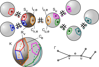
Figure 5. Connected sum of spheres along a tree

Construction 3.2.

We introduce some notation in addition to that of construction 2.8, see Fig. 5. As before, let $\Gamma=(V,E)$ be a tree. Suppose that a simplicial cell $(n-1)$-sphere $S_{v}$ is associated with each node $v\in V$, and for each edge $e\in E$ with an endpoint $v\in V$ there is an admissible vertex $i_{v,e}\in S_{v}$ subject to the following conditions: (1) $\operatorname{link}_{S_{v}}i_{v,e}$ is isomorphic to $\operatorname{link}_{S_{u}}i_{u,e}$ for any edge $e$ with endpoints $v,u$; (2) Vertices $i_{v,e_{1}},i_{v,e_{2}}$ are different and not adjacent in $S_{v}$ for any two edges $e_{1}\neq e_{2}$ emanating from $v$. Then we can form a connected sum along $\Gamma$ as in construction 2.8: $K=\operatorname*{\mathchoice{\raisebox{-10.00012pt}{\leavevmode\resizebox{17.94456pt}{11.94455pt}{\leavevmode\hbox{\set@color$\displaystyle\hash$}}}}{\raisebox{-10.00012pt}{\leavevmode\resizebox{17.94456pt}{11.94455pt}{\leavevmode\hbox{\set@color$\textstyle\hash$}}}}{\raisebox{-10.00012pt}{\leavevmode\resizebox{19.07553pt}{11.36122pt}{\leavevmode\hbox{\set@color$\scriptstyle\hash$}}}}{\raisebox{-10.00012pt}{\leavevmode\resizebox{20.97232pt}{10.97234pt}{\leavevmode\hbox{\set@color$\scriptscriptstyle\hash$}}}}}_{\Gamma}S_{v}$. For each $v\in V$ consider the simplicial subposet

(3.1) $$R_{v}=S_{v}\mathchoice{\raisebox{-10.00012pt}{\leavevmode\resizebox{18.00883pt}{10.81677pt}{\leavevmode\hbox{\set@color$\displaystyle\setminus$}}}}{\raisebox{-10.00012pt}{\leavevmode\resizebox{18.00883pt}{10.81677pt}{\leavevmode\hbox{\set@color$\textstyle\setminus$}}}}{\raisebox{-7.00009pt}{\leavevmode\resizebox{13.7523pt}{7.57175pt}{\leavevmode\hbox{\set@color$\scriptstyle\setminus$}}}}{\raisebox{-5.00006pt}{\leavevmode\resizebox{10.91461pt}{5.40839pt}{\leavevmode\hbox{\set@color$\scriptscriptstyle\setminus$}}}}\bigsqcup_{e\in E,v\in e}\operatorname{star}^{\circ}_{S_{v}}i_{v,e}.$$

This subposet will be called a region. Denote $\operatorname{link}_{S_{v}}i_{v,e}$ by $C_{v,e}$. By construction, $C_{v,e}$ is attached to $C_{u,e}$ if $e=\{v,u\}$. The resulting $(n-2)$-dimensional simplicial subposet of $K$ is denoted by $C_{e}$. Since $i_{v,e}$ is admissible, the subposet $C_{e}\cong C_{v,e}=\operatorname{link}_{S_{v}}i_{v,e}$ is a homological $(n-2)$-sphere as follows from a standard argument in combinatorial topology (see, e.g., [5, Prop.2.2.14]).

We get a collection of $(n-2)$-dimensional cycles $C_{e},e\in E$, dividing the $(n-1)$-sphere $K$ into regions $R_{v},v\in V$. If $e=\{v,u\}$, then $R_{v}$ and $R_{u}$ share a common border $C_{e}$. Note that cycles $C_{e}$ are mutually ordered, meaning that each $C_{e}$ lies at one side of any other cycle. Though the cycles may have common points (as schematically shown on Fig. 5) and even coincide (in this case the region between them coincides with both of them).

On the other hand, any collection of mutually ordered $(n-2)$-dimensional spherical cycles in $K$ determines the representation of $K$ as a connected sum of smaller simplicial cell spheres. A representation $K=\operatorname*{\mathchoice{\raisebox{-10.00012pt}{\leavevmode\resizebox{17.94456pt}{11.94455pt}{\leavevmode\hbox{\set@color$\displaystyle\hash$}}}}{\raisebox{-10.00012pt}{\leavevmode\resizebox{17.94456pt}{11.94455pt}{\leavevmode\hbox{\set@color$\textstyle\hash$}}}}{\raisebox{-10.00012pt}{\leavevmode\resizebox{19.07553pt}{11.36122pt}{\leavevmode\hbox{\set@color$\scriptstyle\hash$}}}}{\raisebox{-10.00012pt}{\leavevmode\resizebox{20.97232pt}{10.97234pt}{\leavevmode\hbox{\set@color$\scriptscriptstyle\hash$}}}}}_{\Gamma}S_{v}$ will be called a slicing.

Define the width of a slicing $\Theta$ to be the maximal number of vertices in its regions:

(3.2) $$\operatorname{wid}(\Theta)\stackrel{{\scriptstyle\text{\tiny def}}}{{=}}\max\{|\operatorname{Vert}(R_{v})|\mid v\in V\}.$$

Define the fatness of a sphere $K$ as the minimal width of all its possible slicings:

(3.3) $$\operatorname{ft}(K)\stackrel{{\scriptstyle\text{\tiny def}}}{{=}}\min\{\operatorname{wid}(\Theta)\mid\Theta\mbox{ is a slicing of }K\}.$$

The essential idea in the proof of Proposition 3.1 is the following.

Lemma 3.3.

Let $K$ be an $(n-1)$-dimensional simplicial cell sphere and $\Lambda\colon\operatorname{Vert}(K)\to\mathbb{Z}^{n}/\pm$ a characteristic function. Let $r$ denote the number of different values of this characteristic function, $r=|\Lambda(\operatorname{Vert}(K))|$. Suppose that $\operatorname{ft}(K)>2r$. Then $(K,\Lambda)$ cannot be represented as a connected sum, along a tree, of simplicial spheres dual to Delzant polytopes.

Proof.

Assume the converse. Then $(K,\Lambda)\cong\operatorname*{\mathchoice{\raisebox{-10.00012pt}{\leavevmode\resizebox{17.94456pt}{11.94455pt}{\leavevmode\hbox{\set@color$\displaystyle\hash$}}}}{\raisebox{-10.00012pt}{\leavevmode\resizebox{17.94456pt}{11.94455pt}{\leavevmode\hbox{\set@color$\textstyle\hash$}}}}{\raisebox{-10.00012pt}{\leavevmode\resizebox{19.07553pt}{11.36122pt}{\leavevmode\hbox{\set@color$\scriptstyle\hash$}}}}{\raisebox{-10.00012pt}{\leavevmode\resizebox{20.97232pt}{10.97234pt}{\leavevmode\hbox{\set@color$\scriptscriptstyle\hash$}}}}}_{\Gamma}(K_{\Psi_{V}(v)},\nu_{v})$, where $\Psi_{V}(v)$ are Delzant polytopes. Forgetting characteristic functions gives a slicing $\Theta$ of $K$. The width of every slicing of $K$ is greater than $2r$ by the definition of fatness. In particular, $\operatorname{wid}(\Theta)>2r$. Thus there exists a node $v$ of $\Gamma$ such that $|\operatorname{Vert}(R_{v})|>2r$.

The region $R_{v}$ is a subcomplex of $K_{\Psi_{V}(v)}$. The restriction of $\Lambda$ to the subset $\operatorname{Vert}(R_{v})$ coincides with the restriction of $\nu\colon\operatorname{Vert}(K_{\Psi_{V}(v)})\to\mathbb{Z}^{n}/\pm$ to $\operatorname{Vert}(R_{v})$. Recall, that $\tilde{\nu}(F)\in\mathbb{Z}^{n}$ is the outward normal vector to the facet $F\in\mathcal{F}(\Psi_{V}(v))=\operatorname{Vert}(K_{\Psi_{V}(v)})$, and $\nu(F)\in\mathbb{Z}^{n}/\pm$ is its class modulo sign. The outward normal vectors to facets of a convex polytope are mutually distinct, thus $|\tilde{\nu}(\operatorname{Vert}{R_{v}})|=|\operatorname{Vert}(R_{v})|$ and, therefore, $|\nu(\operatorname{Vert}(R_{v}))|\geqslant|\operatorname{Vert}(R_{v})|/2$. Thus $|\Lambda(\operatorname{Vert}(R_{v}))|=|\nu(\operatorname{Vert}(R_{v}))|>r$, — the contradiction, since $r$ is the total number of values of $\Lambda$. ∎

So far we may find counterexamples to origami realizability among polytopes, which are $\mathbb{Z}^{n}$-colored with a small number of colors, but whose dual simplicial spheres have large fatness. Of course such examples do not appear when $n=2$ — this would contradict Theorem 1. A simplicial 1-sphere is a cycle graph $\mathcal{C}_{k}$. By considering diagonal triangulations of a $k$-gon, one can easily check that $\mathcal{C}_{k}$ can be represented as a connected sum of several cycle graphs of the form $\mathcal{C}_{4}$ or $\mathcal{C}_{5}$, giving the slicing of width $3$. Hence fatness of any $1$-dimensional simplicial sphere is at most $3$, while any characteristic function takes at least $2$ values, so the conditions of Lemma 3.3 are not satisfied if $n=2$.

The existence of 2-spheres satisfying conditions of Lemma 3.3 is thus our next and primary goal. At first, we prove that any $2$-sphere admits a characteristic function with few values.

Lemma 3.4.

Any simplicial 2-sphere $K$ admits a characteristic function $\Lambda\colon\operatorname{Vert}(K)\to\mathbb{Z}^{3}/\pm$ such that $|\Lambda(\operatorname{Vert}(K))|\leqslant 4$.

Proof.

Four color theorem states that there exists a proper vertex-coloring: $\operatorname{Vert}(K)\to\{\alpha_{1},\alpha_{2},\alpha_{3},\alpha_{4}\}$. Now replace colors by integral vectors $\alpha_{1}\mapsto(1,0,0)$, $\alpha_{2}\mapsto(0,1,0)$, $\alpha_{3}\mapsto(0,0,1)$, $\alpha_{4}\mapsto(1,1,1)$. Any three of these four vectors span the lattice. Therefore the map $\Lambda\colon\operatorname{Vert}(K)\to\mathbb{Z}^{3}/\pm$ thus obtained is a characteristic function. It takes at most $4$ values. ∎

Remark 3.5.

This is a standard trick in toric topology. Classically, it is applied to prove that any simple 3-polytope admits a quasitoric manifold [7].

Though for our purpose we just need $2$-spheres $K$ with $\operatorname{ft}(K)=9$, it seems intuitively clear that in dimension $2$ and higher there exist spheres of arbitrarily large fatness. But it is not a priori clear how to describe such spheres explicitly in combinatorial terms. We present one possible approach below, but some steps of our construction do not generalize to dimensions greater than $2$.

Proposition 3.6.

For any $N>0$ there exists a simplicial 2-sphere $K$ such that $\operatorname{ft}(K)>N$.

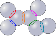
Figure 6. Metric features of a ‘‘thin’’ simplicial sphere

Proof.

The underlying idea is the following. Suppose that a $2$-sphere $K$ is ‘‘thin’’ i.e. $\operatorname{ft}(K)\ll|\operatorname{Vert}(K)|$. Then there exists a slicing $\Theta$ of $K$ into pieces with small numbers of vertices. In particular, the discrete length of any cycle $C_{e}$ in a slicing $\Theta$ should be small. Then the sphere $K$ is ‘‘tightened’’, like the one shown on Fig. 6. It has the feature that small cycles can bound large areas. To measure this property, we introduce a natural metric on $|K|$ in which all edges have length $1$, and then compare the metric space $|K|$ with a ($2$-dimensional) round sphere $\mathbb{S}$ of a constant radius. If there is a bijection $|K|\leftrightarrows\mathbb{S}$ with close Lipschitz constants, then $|K|$ is not thin. The reason why $\mathbb{S}$ suits well for this consideration is that small curves on $\mathbb{S}$ cannot bound large areas, which follows from the isoperimetric inequality.

Quite similar considerations and ideas are used in the theory of planar separators. Some results of this theory can be used to prove Proposition 3.6 directly. If $G$ is a planar graph with $k$ vertices, it is known that there exists a set of $O(\sqrt{k})$ vertices which separates $G$ into two parts of roughly equal size (such separating sets are called planar separators). It is also known that the asymptotic $O(\sqrt{k})$ is the best possible for planar separators [10]. If all $2$-spheres were ‘‘thin’’, then every planar graph would have a separator of size, bounded by some constant, which contradicts the aforementioned asymptotic.

Anyway the deduction of Proposition 3.6 from the known theory requires some additional work, so we give an independent proof. Now that we described the intuitive idea beyond our approach let us get to technical work.

Construction 3.7.

Let $K$ be a $2$-dimensional simplicial complex. Define a (piecewise Riemannian) metric $g$ and measure $\mu$ on $|K|$ in such a way that each triangle $|I|\subset|K|$ becomes an equilateral Euclidian triangle with the standard metric and edge length $1$. Thus the area of each triangle is $\sqrt{3}/4$.

Let $L(\gamma)$ denote the length of a piecewise smooth curve $\gamma$ in $|K|$. If $C\subset K$ is a closed $1$-dimensional cycle (simplicial subcomplex), then, obviously,

(3.4) $$L(|C|)=|\operatorname{Vert}(C)|.$$

A cycle $C$ divides $K$ into two subcomplexes $K_{+}$ and $K_{-}$, each homeomorphic to a closed $2$-disc (we suppose $C\subset K_{+},K_{-}$). Let us estimate the number of vertices in $K_{-}$ in terms of its area ($K_{+}$ is similar). Let $\mathcal{V}_{-},\mathcal{E}_{-},\mathcal{T}_{-}$ denote the number of vertices, edges and triangles in $K_{-}$. By the definition of measure, $\mathcal{T}_{-}=\frac{4}{\sqrt{3}}\mu(|K_{-}|)$. We have $\mathcal{V}_{-}-\mathcal{E}_{-}+\mathcal{T}_{-}=1$ (Euler characteristic of $K_{-}$) and $\mathcal{E}_{-}<3\mathcal{T}_{-}$ (by counting pairs $e\subset t$, where $e$ is an edge and $t$ is a triangle). Therefore,

(3.5) $$\mathcal{V}_{-}\leqslant\frac{8}{\sqrt{3}}\mu(|K_{-}|).$$

Let $\mathbb{S}_{R}$ be a $2$-dimensional round sphere of radius $R$, with the standard metric $g_{s}$ and measure $\mu_{s}$. A piecewise smooth closed curve $\gamma\subset\mathbb{S}_{R}$ without self-intersections divides $\mathbb{S}_{R}$ into two regions $A_{+}$, $A_{-}$. The isoperimetric inequality on a sphere (see e.g. [19, Ch.4]) has the form

(3.6) $$R^{2}L_{s}(\gamma)^{2}\geqslant\mu_{s}(A_{+})\mu_{s}(A_{-}),$$

where $L_{s}(\gamma)$ is the length of $\gamma$. Since $\mu_{s}(\mathbb{S}_{R})=4\pi R^{2}$ we may assume that $\mu_{s}(A_{+})\geqslant 2\pi R^{2}$ (otherwise consider $A_{-}$ instead), thus

(3.7) $$\mu_{s}(A_{-})\leqslant\frac{L_{s}(\gamma)^{2}}{2\pi}.$$

Notice that this inequality does not depend on the sphere radius.

Let $K$ be a $2$-dimensional simplicial sphere and $R,c_{1},c_{2},c_{3},c_{4}$ be positive real numbers. Suppose there exists a bijective piecewise smooth map $f\colon|K|\to\mathbb{S}_{R}$ such that

(3.8) $$c_{1}L(\gamma)\leqslant L_{s}(f(\gamma))\leqslant c_{2}L(\gamma),$$

(3.9) $$c_{3}\mu(\Omega)\leqslant\mu_{s}(f(\Omega))\leqslant c_{4}\mu(\Omega),$$

for each piecewise smooth curve $\gamma\subset|K|$ and measurable set $\Omega\subset|K|$. Numbers $c_{1},c_{2},c_{3},c_{4}$ will be called Lipschitz constants of the map $f$.

Lemma 3.8.

Suppose there exists a mapping $f$ of 2-sphere $K$ into a round sphere $\mathbb{S}_{R}$ with Lipschitz constants $c_{1},c_{2},c_{3},c_{4}$. Let $C$ be a cycle of $K$ dividing it into two closed regions $K_{+}$ and $K_{-}$. If $C$ is contains at most $N$ vertices, then either $K_{+}$ or $K_{-}$ contains at most $\frac{4N^{2}c_{2}^{2}}{\sqrt{3}\pi c_{3}}$ vertices.

Proof.

Among two regions $f(|K_{-}|),f(|K_{+}|)\subset\mathbb{S}_{R}$ let $f(|K_{-}|)$ be the one with the smaller area. Combining (3.4), (3.5), (3.7), (3.8), and (3.9), we get

(3.10) $$\mathcal{V}_{-}\leqslant\frac{8}{\sqrt{3}}\mu(|K_{-}|)\leqslant\frac{8\mu_{s}(f(|K_{-}|))}{\sqrt{3}c_{3}}\leqslant\frac{8L_{s}(f(|C|))^{2}}{2\sqrt{3}\pi c_{3}}\leqslant\frac{4N^{2}c_{2}^{2}}{\sqrt{3}\pi c_{3}},$$

which was to be proved. ∎

Suppose $\operatorname{ft}(K)\leqslant N$. Then by definition there exists a slicing $K=\operatorname*{\mathchoice{\raisebox{-10.00012pt}{\leavevmode\resizebox{17.94456pt}{11.94455pt}{\leavevmode\hbox{\set@color$\displaystyle\hash$}}}}{\raisebox{-10.00012pt}{\leavevmode\resizebox{17.94456pt}{11.94455pt}{\leavevmode\hbox{\set@color$\textstyle\hash$}}}}{\raisebox{-10.00012pt}{\leavevmode\resizebox{19.07553pt}{11.36122pt}{\leavevmode\hbox{\set@color$\scriptstyle\hash$}}}}{\raisebox{-10.00012pt}{\leavevmode\resizebox{20.97232pt}{10.97234pt}{\leavevmode\hbox{\set@color$\scriptscriptstyle\hash$}}}}}_{\Gamma}S_{v}$, encoded by a tree $\Gamma$, such that each region $R_{v}$ has at most $N$ vertices (see construction 3.2). Let us show that the degree of each node $v$ of $\Gamma$ is bounded from above.

Lemma 3.9.

If $\Theta$ is a slicing $K=\operatorname*{\mathchoice{\raisebox{-10.00012pt}{\leavevmode\resizebox{17.94456pt}{11.94455pt}{\leavevmode\hbox{\set@color$\displaystyle\hash$}}}}{\raisebox{-10.00012pt}{\leavevmode\resizebox{17.94456pt}{11.94455pt}{\leavevmode\hbox{\set@color$\textstyle\hash$}}}}{\raisebox{-10.00012pt}{\leavevmode\resizebox{19.07553pt}{11.36122pt}{\leavevmode\hbox{\set@color$\scriptstyle\hash$}}}}{\raisebox{-10.00012pt}{\leavevmode\resizebox{20.97232pt}{10.97234pt}{\leavevmode\hbox{\set@color$\scriptscriptstyle\hash$}}}}}_{\Gamma}S_{v}$ and $\operatorname{wid}(\Theta)\leqslant N$, then $\deg v\leqslant 2(N-2)$ for any node $v$ of $\Gamma$.

Proof.

Denote $\deg v$ by $d$. By construction, the region $R_{v}$ is obtained from a sphere $S_{v}$ by removing $d$ open stars which correspond to the edges of $\Gamma$ emanating from $v$. The complex $R_{v}$ itself can be considered as a plane graph. Denote the numbers of its vertices, edges and faces by $\mathcal{V},\mathcal{E},\mathcal{R}$ respectively. By the definition of the width, we have $\mathcal{V}\leqslant N$. We also have $\mathcal{V}-\mathcal{E}+\mathcal{R}=2$, and $2\mathcal{E}\geqslant 3\mathcal{R}$ (each region has at least $3$ edges). Thus, $\mathcal{V}\geqslant 2+\frac{1}{2}\mathcal{R}$. Notice that each removed open star represents a face of graph $R_{v}$, therefore, $d\leqslant\mathcal{R}\leqslant 2(\mathcal{V}-2)\leqslant 2(N-2)$. ∎

Lemma 3.10.

Let $K$ be a $2$-dimensional simplicial sphere endowed with the map $f$ to the round sphere, satisfying Lipschitz bounds (3.8) and (3.9). For a natural number $N$ set $A=\frac{4N^{2}c_{2}^{2}}{\sqrt{3}\pi c_{3}}$ and $B=2(N-2)$. If $|\operatorname{Vert}(K)|>\max(AB+N,2A)$, then $\operatorname{ft}(K)>N$.

Proof.

Assume the contrary: $\operatorname{ft}(K)\leqslant N$. Then there is a slicing $K=\operatorname*{\mathchoice{\raisebox{-10.00012pt}{\leavevmode\resizebox{17.94456pt}{11.94455pt}{\leavevmode\hbox{\set@color$\displaystyle\hash$}}}}{\raisebox{-10.00012pt}{\leavevmode\resizebox{17.94456pt}{11.94455pt}{\leavevmode\hbox{\set@color$\textstyle\hash$}}}}{\raisebox{-10.00012pt}{\leavevmode\resizebox{19.07553pt}{11.36122pt}{\leavevmode\hbox{\set@color$\scriptstyle\hash$}}}}{\raisebox{-10.00012pt}{\leavevmode\resizebox{20.97232pt}{10.97234pt}{\leavevmode\hbox{\set@color$\scriptscriptstyle\hash$}}}}}_{\Gamma}S_{v}$ in which every region $R_{v}$ has at most $N$ vertices. Consequently, any cycle $C_{e},e\in E$ has at most $N$ vertices. By Lemma 3.8, the cycle $C_{e}$ divides $K$ into two parts, one of which has $\leqslant A$ vertices. Since $|\operatorname{Vert}(K)|>2A$, the other part has $>A$ vertices. Assign a direction to each edge $e$ of $\Gamma$ in such a way that $e$ points from the larger component of $K\smallsetminus C_{e}$ to the smaller, where the ‘‘size’’ means the number of vertices.

$\Gamma$ is a tree, therefore there exists a source, i.e. a node $u$ from which all adjacent edges emanate. Speaking informally, this node represents a ‘‘big sized bubble’’, meaning that the part of a sphere, lying across each border has a small size. Let $d$ denote the degree of the chosen node $u$. Denote by $\Gamma_{1},\ldots,\Gamma_{d}$ the connected components of the graph $\Gamma\smallsetminus u$. By Lemma 3.9 we have $d\leqslant B$. By the construction of the directions of edges, $\left|\operatorname{Vert}(\bigsqcup_{\Gamma_{i}}R_{v})\right|\leqslant A$ for each $\Gamma_{i}$. Thus $|\operatorname{Vert}(K)|\leqslant|\operatorname{Vert}(R_{u})|+\sum_{i=1}^{d}\left|\operatorname{Vert}(\bigsqcup_{\Gamma_{i}}R_{v})\right|\leqslant N+AB$ — the contradiction. ∎

Lemma 3.11.

For any $N>0$ there exists a $2$-dimensional simplicial sphere $K$ such that:

1. There exists a piecewise smooth map $f\colon|K|\to\mathbb{S}_{R}$ satisfying Lipschitz bounds (3.8) and (3.9) for some constants $c_{1},c_{2},c_{3},c_{4},R>0$

2. $|\operatorname{Vert}(K)|>\max(AB+N,2A)$, where $A$ and $B$ are defined in Lemma 3.10.

Proof.

Start with the boundary of a regular tetrahedron with edge length $1$: $L=\partial\Delta^{3}$. The projection from the center of $L$ to the circumsphere $f\colon L\to\mathbb{S}_{R}$ is obviously Lipschitz for some constants $c_{1},c_{2},c_{3},c_{4}>0$. Now subdivide each triangle of $|L|$ into $q^{2}$ smaller regular triangles as shown on Fig. 7.

Figure 7. Subdivision of a regular triangle.

This results in a simplicial complex $L_{(q)}$. As a space with metric and measure $|L_{(q)}|$ is homothetic to $|L|$ with a linear scaling factor $q$ (recall that the metric on simplicial complexes is introduced in such way that each edge has length $1$). Thus there exists a map $f_{(q)}\colon|L_{(q)}|\to\mathbb{S}_{qR}$ with the same Lipschitz constants as $f$. The number of vertices $|\operatorname{Vert}(L_{(q)})|$ can be made arbitrarily large.

∎

Lemmas 3.11 and 3.10 conclude the proof of Proposition 3.6. ∎

Remark 3.12.

Actually, in the proof of Lemma 3.11 we could have started from any simplicial sphere $L$, take any piecewise smooth map $f\colon|L|\to\mathbb{S}_{R}$, find Lipschitz constants $c_{2},c_{3}>0$ (they exist by the standard calculus arguments), and then apply the same subdivision procedure. We used the boundary of a regular simplex, because in this case Lipschitz map is constructed easily and allows for an explicit computation.

We give a concrete example of a quasitoric manifold which is not toric origami, by performing this computation. The calculations themselves are elementary thus omitted. It is sufficient to construct a simplicial sphere for $N=8$. For a projection map from the boundary of a regular tetrahedron to the circumscribed sphere we have Lipschitz constants $c_{2}=3$, $c_{3}=\frac{1}{3}$. Thus $\max(AB+N,2A)\approx 15251.14$. Subdivide each triangle in the boundary of a regular tetrahedron in $q^{2}$ small triangles where $q\geqslant 88$. This gives a simplicial sphere $K$ with at least $15490$ vertices and the same Lipschitz constants as $\partial\Delta^{3}$. Thus $\operatorname{ft}(K)>8$. Now take the dual simple polytope $P$ of $K$, consider any proper coloring of facets in four colors and assign a characteristic function $\Lambda$, as described in Lemma 3.4. This gives a characteristic pair $(P,\Lambda)$, whose corresponding quasitoric manifold is not toric origami.

Of course, all our estimations are very rough, and, probably, there are better ways to construct fat spheres. For sure, there exist $2$-spheres of fatness $9$ with less than $15490$ vertices.

Remark 3.13.

Note that in dimension $3$ and higher there is no simplicial subdivision of a regular simplex into smaller regular simplices. This is one of two places in the proof, where the dimension restriction is crucial. The second place is the Four color theorem in Lemma 3.4.

Proposition 3.1 proves Theorem 2 for $n=3$. Now we need to make the remaining cases $n>3$.

Proposition 3.14.

There exist quasitoric manifolds of any dimension $2n$, $n>3$, which are not toric origami.

Proof.

Let $M_{(P,\Lambda)}$ be any quasitoric manifold, which is not toric origami. Take the product of $M_{(P,\Lambda)}$ with $S^{2}$ (the circle $T^{1}$ acts on $S^{2}$ by axial rotations). On the level of orbit spaces, this corresponds to multiplying $P$ with a closed interval $\mathbb{I}\subset\mathbb{R}$. We claim that quasitoric manifold $M_{(P,\Lambda)}\times S^{2}$ is not toric origami. If $M_{(P,\Lambda)}\times S^{2}$ were a toric origami manifold, then all its characteristic submanifolds should be toric origami as well (see construction 1.10). But $M_{(P,\Lambda)}$ is one of them. This gives a contradiction. Thus taking products with $S^{2}$ produces examples for all $n>3$. ∎

Remark 3.15.

Sphere $S^{2}$ is the simplest example of a quasitoric manifold. In the proof of Proposition 3.14 we could have used any other quasitoric manifold instead of $S^{2}$. If $M_{(P,\Lambda)}$ and $M_{(P^{\prime},\Lambda^{\prime})}$ are quasitoric manifolds and one of them is not toric origami, then the quasitoric manifold $M_{(P,\Lambda)}\times M_{(P^{\prime},\Lambda^{\prime})}=M_{(P\times P^{\prime},\Lambda\oplus\Lambda^{\prime})}$ is not toric origami as well.

Remark 3.16.

On the other hand, new toric origami manifolds can be produced from a given one in a similar way as we used for constructing non-examples. It is easy to observe that if $M$ is a toric origami manifold and $M^{\prime}$ is a toric symplectic manifold, then $M\times M^{\prime}$ is again a toric origami manifold. We would also like to mention that projective bundles over toric origami manifolds are again toric origami manifolds. More precisely, if $M^{2n}$ is toric origami, and $L_{1},\ldots,L_{k}$ are complex line bundles over $M$, each having an $S^{1}$ action on fibers, then the projectivization

$$\tilde{M}=P\left(\bigoplus_{j=1}^{k}L_{j}\oplus\underline{\mathbb{C}}\right)$$

with the induced action of $T^{n}\times(S^{1})^{k}$ is also a toric origami manifold.

4. Discussion and open questions

4.1. Asymptotically most of simplicial $2$-spheres are fat

We already mentioned a relation of our study to the theory of planar separators in Section 3. We also want to mention another connection to the theory of random infinite planar maps. This rapidly developing part of probability theory aims, among other things, to give a firm foundation for some facts in statistical physics and quantum gravity. The basic idea of this study is the following [14, 15]. Fix a number $k$, a parameter of the whole construction. For a given $n$ consider all possible (rooted) plane $k$-angulations with $n$ faces. For $k=3$, these are roughly the same as simplicial spheres. Every plane graph has a standard metric, turning it into a metric space. By letting the number of faces tend to infinity, and renormalizing the diameter of graphs in a correct way, one considers the limits of converging sequences of graphs. The limits are taken with respect to the Gromov–Hausdorff metric defined on the set of isometry classes of metric spaces.

Since there is only a finite number of such graphs with a fixed number $n$ of faces, we can take a uniform distribution on this set of graphs. The uniform distributions on the sets of prelimit metric spaces give rise to a limiting distribution, which is viewed as a random compact metric space (of course, here we omit a lot of technicalities, needed to state everything precisely). The resulting random metric space is called a Brownian map and considered as a good $2$-dimensional analogue of the Brownian motion.

A wonderful thing is that a Brownian map does not actually depend on the parameter $k$, if $k$ is either $3$ or even [15]. It is also known that the Brownian map is almost surely homeomorphic to a $2$-sphere [13]. This suggests the following

Claim 4.1.

For each $N>0$ almost all simplicial $2$-spheres $K$ have $\operatorname{ft}(K)>N$. More precisely, if $A_{n}$ denotes the set of all simplicial $2$-spheres with $\leqslant n$ triangles, and $B_{n,N}\subset A_{n}$ the subset of simplicial spheres having $\operatorname{ft}(K)>N$, then

$$\lim_{n\to\infty}\frac{|B_{n,N}|}{|A_{n}|}=1.$$

The reason is as follows (cf. [14, Cor.5.3]). If there were a lot of ‘‘thin’’ simplicial spheres, they all would have bottlenecks — small cycles, dividing them into macroscopic regions. After taking a limit as $n\to\infty$ and rescaling the metric, these bottlenecks would collapse to points. Thus the limiting metric space would be non-homeomorphic to a sphere with non-zero probability.

Therefore, for most of simple combinatorial 3-polytopes $P$ there exists a characteristic function $\Lambda$ such that $M_{(P,\Lambda)}$ is not toric origami.

4.2. Orbit spaces of toric origami manifolds

We may ask a more intricate question.

Problem 1.

Find a simple polytope $P$ such that any quasitoric manifold $M_{(P,\Lambda)}$ over $P$ is not equivariantly homeomorphic to a toric origami manifold.

This question is motivated by the following fact. There exist a simple 3-polytope $P$ such that any quasitoric manifold $M_{(P,\Lambda)}$ over $P$ is not equivariantly homeomorphic to a symplectic toric manifold. Stating shortly: there exist combinatorial types of simple 3-polytopes which do not admit Delzant realizations. It was proved in [8] that any 3-dimensional Delzant polytope has at least one triangular or quadrangular face. Consequently, in particular, a dodecahedron does not admit a Delzant realization.

An origami template is a generalization of a single Delzant polytope, thus a realizability of a given combinatorial polytope by an origami template is a more complicated task. Problem 1 can be restated in different terms: are there any combinatorial restrictions on the orbit spaces of toric origami manifolds?

4.3. Fat simplicial spheres in higher dimensions

The examples of non-origami quasitoric manifolds in high dimensions were constructed from the $3$-dimensional case. On the other hand, Lemma 3.3 applies for any dimension. The problem of finding higher-dimensional polytopes whose dual spheres have large fatness may be of independent interest.

Actually, even if we find such a fat sphere, to make use of the developed technique we should also construct a characteristic function with a small range of values. This constitutes a certain problem, since characteristic function may not even exist, if $n\geqslant 4$ (this happens for dual neighborly polytopes, see [7]). Nevertheless, there is a big class of simplicial $(n-1)$-spheres, so called balanced spheres, which admit a proper vertex-coloring in $n$ colors. Such colorings give rise to characteristic functions, which have exactly $n$ values, i.e. minimal possible. Such characteristic functions and the corresponding quasitoric manifolds were called linear models in [7]. Passing to a barycentric subdivision makes every simplicial sphere into a balanced sphere. We suppose that passing to a barycentric subdivision does not strongly affect the fatness. If so, given any fat sphere dual to a simple polytope, one can pass to its barycentric subdivision, provide it with a linear model characteristic function, and finally obtain a quasitoric manifold which is not toric origami.

4.4. Minimizing the range of characteristic function

Another problem, which naturally arises from Lemma 3.3 is to find, for a given polytope $P$, a characteristic function $\Lambda$ with the minimal possible range of values $|\Lambda(\mathcal{F}(P))|$, if at least one characteristic function is known to exist. This minimal number seems to be an analogue of Buchstaber invariant (see the definition in [11] or [1]), as was noted to us recently by N. Erokhovets. It may happen that an interesting theory hides beyond this subject.

4.5. Toric varieties

There exist obstructions to origami realizability, other than those described in section 3. If a weighted simplicial sphere $K$ can be represented as a connected sum, along a tree, of simplicial spheres dual to Delzant polytopes, this does not mean automatically that $K$ corresponds to an origami template. The reason is that a convex polytope contains more information than its normal fan (or, in our terminology, dual weighted simplicial sphere). It can be impossible to assemble an origami template from a collection of Delzant polytopes, even if their dual weighted spheres suit together well.

Such situations appeared when we tried to answer the following

Problem 2.

Does there exist a compact smooth toric variety, which is not equivariantly homeomorphic to a toric origami manifold?

Any projective toric variety corresponds to a convex polytope. Thus any smooth projective toric variety is a symplectic toric manifold, which is a particular case of toric origami. Thus, to prove the conjecture, one should consider non-projective examples. Translating the problem into combinatorial language, the task is to find a complete smooth fan, which is not a normal fan of any polytope and, moreover, not dual to any origami template. The simplest non-polytopal fan is the fan corresponding to a famous non-projective Oda’s 3-fold [18, p.84]. So it is natural to start with a more concrete question:

Problem 3.

Is Oda’s 3-fold a toric origami manifold?

Even this question happens to be rather non-trivial and cannot be solved solely by the method developed in this paper.

4.6. Origami manifolds which are not quasitoric

In section 1 we mentioned that a toric origami manifold $M_{O}$ is not quasitoric if its template graph has cycles. Even if the orbit space of $M_{O}$ is contractible, the manifold $M_{O}$ may not be quasitoric. The simplest example of this kind is the sphere $S^{4}$ (example 1.9). The orbit space of $S^{4}$ is a 2-gon, shown on Fig. 2, which is not a convex polytope. Excluding situations of these two kinds we may ask the following question.

Problem 4.

Let $M_{O}$ be a simply connected toric origami manifold and suppose that the dual simplicial sphere of its orbit space is a simplicial complex. Is the manifold $M_{O}$ quasitoric?

In other words, does the orbit space of a simply connected toric origami manifold admit a convex realization, provided that its dual simplicial sphere is a simplicial complex?

References

- [1] A. Ayzenberg, Buchstaber numbers and classical invariants of simplicial complexes, arXiv:1402.3663.
- [2] A. Ayzenberg, M. Masuda, S. Park, H. Zeng, Cohomology of toric origami manifolds with acyclic proper faces, preprint arXiv:1407.0764.
- [3] V. M. Buchstaber, T. E. Panov, Combinatorics of Simplicial Cell Complexes and Torus Actions, Proceedings of the Steklov Institute of Mathematics, Vol. 247, 2004, pp. 1–17.
- [4] V. M. Buchstaber, T. E. Panov, N. Ray, Spaces of polytopes and cobordism of quasitoric manifolds, Mosc. Math. J., 7:2 (2007), pp. 219–242.
- [5] V. Buchstaber and T. Panov, Toric Topology, preprint arXiv:1210.2368.
- [6] A. Cannas da Silva, V. Guillemin and A. R. Pires, Symplectic Origami, IMRN 2011 (2011), 4252–4293, preprint arXiv:0909.4065.
- [7] M. Davis, T. Januszkiewicz, Convex polytopes, Coxeter orbifolds and torus actions, Duke Math. J., 62:2 (1991), 417–451.
- [8] C. Delaunay, On Hyperbolicity of Toric Real Threefolds, IMRN International Mathematics Research Notices 2005, No. 51.
- [9] T. Delzant, Hamiltoniens periodiques et image convex de l’application moment, Bull. Soc. Math. France 116 (1988), 315–339.
- [10] H. N. Djidjev, On the problem of partitioning planar graphs, SIAM. J. on Algebraic and Discrete Methods, 3(2), 229–240.
- [11] N. Erokhovets, Buchstaber Invariant of Simple Polytopes, arXiv:0908.3407.
- [12] T. Holm and A. R. Pires, The topology of toric origami manifolds, Math. Research Letters 20 (2013), 885–906, preprint arXiv:1211.6435.
- [13] J.F. Le Gall and F. Paulin, Scaling limits of bipartite planar maps are homeomorphic to the 2-sphere, Geom. Funct. Anal. 18 (2008), 893–918, preprint arXiv:math/0612315.
- [14] J.F. Le Gall, Large random planar maps and their scaling limits, Proceeedings 5-th European Congress of Mathematics, Amsterdam 2008. EMS, Zurich 2010.
- [15] J.F. Le Gall, Uniqueness and universality of the Brownian map, Ann. Probab. Volume 41, Number 4 (2013), 2880–2960, preprint arXiv:1105.4842.
- [16] Z. Lu and T. Panov, Moment-angle complexes from simplicial posets, Cent. Eur. J. Math. 9 (2011), no.4, 715-730, preprint arXiv:0912.2219.
- [17] M. Masuda and S. Park, Toric origami manifolds and multi-fans, to appear in Proc. of Steklov Math. Institute dedicated to Victor Buchstaber’s 70th birthday, arXiv:1305.6347.
- [18] T. Oda, Convex Bodies and Algebraic Geometry: An Introduction to the Theory of Toric Varieties, Springer-Verlag, Berlin–Heidelberg, 1988.
- [19] R. Osserman, The isoperimetric inequality, Bull. of AMS, Vol.84, N.6, 1978.
- [20] T. Yoshida, Local torus actions modeled on the standard representation, Advances in Mathematics 227 (2011), pp. 1914–1955.
- [21] G. M. Ziegler. Lectures on Polytopes. Springer-Verlag, New York, 2007.