Exponent dependence measures of survival functions and correlated frailty models
J. Bendela, D. Doblerb, A. Janssenc,∗††∗ Corresponding author; full address: Mathematical Institute, University of Düsseldorf, Universitätsstr. 1, 40225 Düsseldorf, Germany; Telephone number: 0049 211 8112165
E-mail addresses: dennis.dobler@uni-duesseldorf.de (D. Dobler), jens.bendel@uni-duesseldorf.de (J. Bendel), janssena@uni-duesseldorf.de (A. Janssen)
aDepartement of Mathematics and Statistics, University of Reading, UK
bInstitute of Statistics, Ulm University, Germany
cMathematical Institute, University of Düsseldorf, Germany
Abstract
The present article studies survival analytic aspects of semiparametric copula dependence models
with arbitrary univariate marginals.
The underlying survival functions admit a representation via exponent measures
which have an interpretation within the context of hazard functions.
In particular, correlated frailty survival models are linked to copulas.
Additionally, the relation to exponent measures of minumum-infinitely divisible distributions
as well as to the Lévy measure of the Lévy-Khintchine formula is pointed out.
The semiparametric character of the current analyses
and the construction of survival times with dependencies of higher order are carried out in detail.
Many examples including graphics give multifarious illustrations.
keywords:
Copula , correlated frailty model , survival analysis , multi-dimensional hazard function
, dependence measure , infinite divisibility
1 Introduction
Multivariate semiparametric dependence models have been successfully developed during the past decades.
We refer to the huge amount of copula literature; see Joe (1997) and Nelsen (2006) among others.
It is well-known that Sklar’s (1959) theorem allows
to separate a multivariate distribution in a copula dependence part and marginal distribution functions
which are often considered as nuisance parameters.
On the other hand, failure rates and hazard functions are very meaningful in survival analysis for dependent life time data.
The famous Cox regression model specifies the dependence via exponential hazard dependence models
with baseline hazard nuisance parameters, cf. Cox (1972).
The hazard-based Cox models were extended by correlated frailty models
which allow hazard dependence including flexible individual effects for life times;
see Duchateau and Janssen (2008), Hougaard (2000), Wienke (2011) and Aalen et al. (2008).
The shared frailty model appears as a special case whose connection to Archimedean copulas was pointed out by
Kimberling (1974), Marshall and Olkin (1988), Oakes (1989) and McNeil and Nes̆lehová (2009);
see also Genest and McKay (1986), Duchateau and Janssen (2008) and Völker (2010) for further discussions.
It is the aim of this paper to study the multivariate dependence structure from the survival analysis point of view,
in particular for the survival functions of copulas.
We thereby like to connect the copula dependence structure with hazard quantities.
Our hazard dependence functions (and dependence measures) have a direct interpretation in survival analysis
and they may serve as parameters for statistical dependence modeling.
Recall that, under continuity, univariate hazard measures are exponent measures of survival functions ,
i.e. for continuous ;
see Gill (1993) and Dabrowska (1996) for exponents of multivariate survival functions.
The article is organized as follows.
The basics of multivariate survival analysis are presented in Section 2.
Along with the work of Gill (1993) and Dabrowska (1996)
the exponent representation of Lemma 2.1 for multivariate survival functions is recalled
which later leads to so-called exponent measures of dependence.
It is also connected to the concept of “local dependence hazard” parameters studied earlier by Janssen and Rahnenführer (2002) in the bivariate case.
Section 3 links the exponent dependence measure
to earlier analyzed exponent measures of Resnick (1987) for minumum-infinitely divisible distributions in extreme value theory.
In Section 4 signed exponent measures of dependence are studied in detail
for survival functions of correlated frailty models.
These are introduced as multivariate exponentially distributed variables with random scales .
In terms of the Laplace transform of W explicit analytic formulas are derived for their densities, hazards and exponent measures,
in particular, for the special examples of dependent or log-normal random scales .
If W is sum-infinitely divisible, then the dependence exponent measures are linked to the Lévy measure
given by the Lévy-Khintchine formula for W; see Section 5.
Section 6 is devoted to semiparametric survival models with arbitrary marginals.
It is shown that the exponent dependence measures can be parametrized in a copula manner.
The underlying parametrized dependence quantities are later visualized
for some examples of correlated frailty models; see Figures 1 to 4.
Together with the motivation given by the upcoming equations (2.7)–(2.9)
the plots have a meaningful hazard-based interpretation regarding the quality of dependence.
For instance, there exist copulas with overall proportional hazard dependence for all bivariate submodels
but without dependence for exponent measures of higher order.
On the contrary, copula models can be constructed
for which all proper subvectors are independent but the whole vector has a non-trivial dependence measure;
see Section 7 for an elaboration of such models via hazard functions.
Additional examples and graphs as well as some technical details are presented in the appendix to this article.
2 Survival Functions
A copula is a distribution function on the -dimensional unit cube with uniformly distributed marginals.
It is well known that copulas describe the dependence structure of -valued random variables
whereas the distributions of the one-dimensional marginals are often regarded as
nuisance parameters in statistics.
In this paper we will study survival functions and their corresponding survival copulas which are very useful in risk and survival analysis
when multivariate failure rates and hazard rates have a concrete meaning; see for instance Gill (1993) and Dabrowska (1996).
For a pair of random variables the hazard rate dependence approach is a meaningful description of the
survival copula dependence structure; see Janssen and Rahnenführer (2002).
They showed that an exponential dependence measure exists which naturally explains the
dependence structure.
At other times we like to apply the copula concept in order to convert all marginals to uniform distributions,
eliminating all nuisance parameters in doing so.
Throughout let denote a random variable
with -dimensional continuous distribution function
and let and , ,
be the marginal distribution and survival functions.
The -dimensional survival function is given by
(2.1)
To fix the notation let () denote the left-sided continuous inverse distribution (survival)
function of . In our continuous case the variables
(2.2)
both define copulas on :
The distribution function of (a) is simply called copula of T and similarly
the distribution function of (b) is defined as the survival copula of T, cf. Nelsen (2006), Section 2.6, as well as McNeil and Nes̆lehová (2009).
We see that
is just the survival function (2.1) of .
To avoid further confusions we like to stress the necessity to clearly distinguish
between the survival copula and the survival function of the copula .
These concepts lead to different dependence models for survival times.
Furthermore, the survival function and the survival copula are connected by
(2.3)
Thus, every survival function can easily be reproduced by its survival copula and the continuous
marginal survival functions.
In order to study multivariate survival functions in more detail we first recall elements
of univariate survival analysis for a continuous real valued random variable .
For a detailed introduction we refer to the books by Klein and Moeschberger (2003) and Aalen et al. (2008).
If we put , then there exists a so-called hazard measure
on the interval with cumulative hazard function given by
(2.4)
The hazard measure can be viewed as univariate exponent measure of the survival function.
Whenever has a Lebesgue density then
holds for the hazard rate .
For example, the hazard measure of a standard exponentially distributed random variable is just
the Lebesgue measure on .
In the next step exponential representations of multivariate survival functions are studied which are used to extend the univariate hazard formula (2.4).
Special models and exponent measures are examined in the proceeding sections.
Consider an index set . Then
denotes the domain of the survival function of the marginals .
The following Lemma
is written in the spirit of Gill (1993) who studied the survival function in the context of product integrals.
The proof follows by induction;
see also Dabrowska (1996), equation (1.1).
Lemma 2.1.
Consider the continuous survival function of
and let denote the survival function of the -dimensional marginal vector .
Define for a single subset
the function on as the marginal
. For every , ,
there exists a positive function
which is uniquely determined by the following representation of marginal survival functions.
For each index set the marginal survival function
admits the factorization
(2.5)
where the product is taken over all subsets
.
We call
the dependence parts of order which
are unique on their domain.
For a singleton the cumulative hazard function corresponds to an exponent measure,
. In the same manner we can, for all with , define an exponent function on the domain
by
(2.6)
As we will see, the higher dimensional exponents are typically linked to signed exponent measures of dependence.
As motivation and in order to give a proper interpretation let us first recall
the hazard dependence approach for and dimension :
Janssen and Rahnenführer (2002)
pointed out that is a signed exponent measure.
If has a density then
also has a density on
and (2.5) writes as
(2.7)
Recall again
the interpretation of the univariate hazard
function
as failure rate.
Under smoothness of and for small we approximately have,
given the event ,
(2.8)
In the same way has an interpretation as “local dependence hazard” of
and .
For smooth densities, and small Janssen and Rahnenführer (2002) verified that
(2.9)
holds.
They also showed that
the exponent dependence measure and its density are extremely useful for testing independence for
randomly censored survival models.
In their work the reader will find a lot of examples for hazard dependence structures
and efficient tests for independence of the marginals at dimension 2; see also Section 7 below.
3 Exponent dependence measures of minimum-infinitely divisible distributions
In this section we link the exponents of dependence to already known measures of dependence.
Observe that in extreme value theory minimum-infinitely divisible distributions allow related exponent representations.
A distribution on with survival function is called minimum-infinitely divisible if is a survival function for each .
For obvious reasons we will focus on the copula case.
It is well known (cf. Resnick, 1987, Section 5.3, switching from the to the operation)
that, under minimum-infinite divisibility, there exists a possibly unbounded exponent Radon measure on with
(3.1)
where is the complement of in
and .
To get an impression of (3.1) consider the bivariate case :
Example 3.1.
(a) Let be the survival function of the independence copula of dimension .
Then lies on the upper
boundary of with , ,
and being the Dirac measure in 1.
(b) If is minimum-infinitely divisible and given by (3.1) then
holds for all if is continuous.
Remark 3.2.
(a) The distribution of two non-negative random variables with local dependence hazard
(cf. Proposition 4.8 and the discussion after
Lemma 2.1)
is minimum-infinitely divisible iff
is non-negative. Joe (1997), Theorem 2.7, proves this and a
similar result for arbitrary dimensions .
(b) Part (b) of Example 3.1 is a special case of the following Proposition 3.3,
from which we conclude that
the behaviour of in the interior of determines the dependence structure of .
Proposition 3.3.
Let be the survival function of a continuous minimum-infinitely divisible copula given by (3.1).
For each index set the function given by
(2.6) is a measure generating function of a positive measure on with
(3.2)
where
is the image measure of the canonical projection w.r.t. the restricted measure of
on .
Proof.
The proof relies on an inclusion-exclusion principle type of argument (also known as the sieve formula or Sylvester-Poincaré equality).
For observe that
and
hold, where denotes the indicator function of a set .
Moreover, is the exponent measure (3.1) of the -dimensional marginal survival function .
Hence, and can be identified step by step. For the univariate hazard measures are obtained.
In genereal, when all with , , are identified,
then the remaining part must be given by (3.2).
Note that is completely determined by for .
∎
Remark 3.4.
Suppose that has a minimum-infinitely divisible distribution with exponent measure given by (3.1)
and that is continuous.
The following statements are equivalent (cf. Resnick (1987), Section 5.5, for the equivalence of and ).
1.
The components are independent random variables.
2.
The components are pairwise independent, i.e. and are independent random variables for every .
3.
For every with the bivariate exponent measure given by (2.6) is equal to zero.
4.
For every with the exponent measure given by (2.6) is equal to zero.
4 Dependence measures for correlated frailty models
As explained in Section 2 the univariate marginals are irrelevant when the dependence structure is studied
within a semiparametric context. This is a chance to choose in a first step the marginals in a convenient
way as we did in (2.2). In a second step the marginals may be transformed if necessary. For this reason
we will first introduce a correlated frailty model for special marginals which gives more insight in the
underlying dependence structure. Originally the frailty concept shows up in multivariate survival
analysis when individual hazard effects are modeled by an additional factor attached to famous Cox
models; see Andersen et al. (1993) for further references.
The idea to link several individuals via the same factor leads to shared frailty models
and closely related Archimedean copulas; see Section 1 for references to this connection.
Our next example shows that these particular copulas fit very well in the context of survival copulas.
Example 4.1.
Let be the following generator of an Archimedean copula :
is a nonincreasing and continuous function satisfying
, and strictly decreasing
on the interval . Then is given by
Obviously, define marginal survival functions. If is
distributed according to the above Archimedean copula with generator then by (2.3)
(4.1)
is the survival function of with survival function
of the marginals.
Furthermore, is the survival copula of T.
We see that the above choice of marginals yields a pleasant form of the survival function.
Remark 4.2.
Okhrin et al. (2013) study hierarchical Archimedean copulas,
which extend the class of Archimedean copulas.
They show that any hierarchical Archimedean copula can be uniquely recovered from all bivariate marginal copula functions.
We now introduce a class of correlated frailty models which admit meaningful hazard dependence structures.
The explanation below Lemma 4.6 exhibits the relation to the Archimedean copula structure (4.1).
Let denote a probability measure on with Laplace transform
It will turn out that is a meaningful quantity for the multivariate survival time X defined as follows.
Definition 4.3.
Let and denote two independent -dimensional random vectors with law
and let be i.i.d. standard exponentially distributed. The random vector X given by
(4.2)
is then called a correlated frailty model based on .
Remark 4.4.
In multivariate survival analysis the concept of frailty was originally introduced
with equal variables (called shared frailty model)
to model unobserved heterogeneity.
For a more detailed discussion of the univariate proportional frailty model,
including surveys of the model for different distributions of the frailty variable and extensions,
we refer to the books by
Wienke (2011), Chapter 3,
Duchateau and Janssen (2008) and
Aalen et al. (2008), Chapter 6,
as well as to the article by Völker (2010).
In contrast to the shared frailty model, the correlated frailty model is more flexible
and it takes the dependency structure of the ’s into account.
Usually the definitions of frailty models are given in terms of the hazard rates of .
Thus it is possible to include a baseline hazard as well as covariates in the model.
As the focus of this article lies on dependence structures we omit covariates and choose (justified by the copula approach)
a possibly simple baseline hazard equal to one. These simplifications lead to the definition given by (4.2).
A brief introduction to the correlated frailty model for the bivariate case (d = 2)
and its relation to Cox models can be found in the book by Wienke (2011), Section 5.1.
The correlated frailty model is a multivariate exponential scale model with random scale parameter W.
Any strictly increasing transformation of the coordinates of X leads to a conditional Cox model given W.
Subsequently, it turns out that the structure of (4.2) is closely connected to the exponential family given by
(4.3)
The following analytic properties of Laplace transforms and exponential families are well known; see Barndorff-Nielsen (1978).
Remark 4.5.
(a) The Laplace transform is a positive analytic function on .
(b) Consider and, for each , let be a multiplicity.
Let with whenever holds.
Then
(4.4)
(c) Suppose that is given by a probability measure on .
Via projection we may assume that the underlying joint probability space is a product space
with product measure and
is the identity of the second component. Then can naturally be regarded as
random vector under , shortly under .
Lemma 4.6.
The following results hold for the correlated frailty model X.
(a) The survival function coincides with the Laplace transform for all
.
(b) The distribution of X is concentrated on . On this set it has the analytic density
(4.5)
(c) For and the -th marginal hazard measure
is given by with -th univariate hazard rate
(4.6)
Consider the special case that coincide, i.e. X is a shared frailty model.
If denotes the univariate Laplace transform of ,
then the survival function of X collapses to
and (4.2) corresponds to the transformation of the Archimedean copula (4.1)
given by the completely monotone function .
by the independence of the ’s.
(b) Whenever a density exists, we have
by part (a) for each .
Formal differentiation of gives the analytic left-hand side of (4.5)
and the result follows.
(c) The first part follows since
Then its derivative can be calculated by (4.4).
∎
We see that distributional quantities like and are linked to and its derivatives.
To see that the hazard quantities also rely on , consider as in (2.5).
Then we have
with first order terms .
The higher order terms for are now studied in detail and linked to (2.7).
Throughout, the following notation is used.
Let denote a function with existing derivatives of sufficiently high order.
Introduce for the following notation: For
is the function given by when the coordinates , , are zero.
Similarly, for a given we denote by the -dimensional vector with zero entries for all indices
and with entries else.
For we also introduce
and
Lemma 4.7.
The logarithm of the survival function of a correlated frailty model is given by
(4.7)
Proof.
Since holds, the main theorem of multivariate calculus yields (4.7) by induction over .
∎
This result identifies the exponents for . We have
(4.8)
where
Similarly as for Lemma 2.1 the proof is given by induction over the dimension .
The first order (hazard) measures are described in (4.6) by the exponential family (4.3).
In our context are measure generating functions of signed measures.
Here, the bivariate measures are determined by particularly interesting densities:
Proposition 4.8.
Consider , and .
Then the density of the signed measure is given by the covariance structure of the exponential family:
Remark 4.9.
(a) The local hazard dependence density in (2.9)
has now an interpretation in terms of correlations for the correlated frailty model.
(b) Higher order expressions of (4.8) are similar but more complicated.
The role of higher order exponent measures is discussed in Section 6.
Combining (4.3) and (4.4),
we see that the first term corresponds to the expected value
whereas the second term is just the product ;
see also (4.6).
∎
In life science analysis two risk components can be modeled as a minimum of two survival variables:
For example, we could think of individuals who are exposed to two different lethal risk factors.
Then the survival times are the first occurrences of one of the competing events.
This concept goes well with the correlated frailty model:
Lemma 4.10.
Let W and be two -dimensional frailty variables
with correlated frailty models
for i.i.d. standard exponentially distributed .
Let and denote the survival functions of and , respectively.
(a) We have equality in distribution of
Here denotes the component-wise minimum operation.
Thus, the class of correlated frailty models is closed w.r.t. the minimum operation.
(b) The following conditions (i)-(ii) are equivalent.
(i)
The correlated frailty model
has the survival function .
(ii)
W and are independent.
The proof is obvious. Note, that the conditional survival function of
at t given is .
The independence of W and is equivalent to the product of
Laplace transforms which corresponds to the products of survival functions; see Lemma 4.6.
Example 4.11.
Let have a multivariate normal distribution
with mean vector zero and non-singular covariance matrix .
(a) Correlated frailty models with the following frailty variables W
are uniquely determined by the collection of bivariate distributions , ,
i.e. by the covariances :
1.
Frailty variables with -distributed marginals:
.
2.
Frailty variables with log-normal marginals: .
(b) The correlated frailty vector given by (1) or (2) has independent components
iff has diagonal form.
In contrast to Example 4.11 there exist correlated frailty models with pairwise independent components of X but higher order dependence.
For instance let be pairwise independent but not totally independent.
Then has the form
with trivial exponent measures for .
See Section 7 for a related discussion which systematically characterises copulas
having only dependencies of the highest order.
Part (a) of the following example continues Example 4.11(a)(i) for the special case :
Example 4.12.
(a) Let follow a multivariate normal distribution with mean
for and covariance matrix
and let denote the correlation coefficient of and .
Consider the correlated frailty model (4.2) with frailty variables , .
Explicit formulas and their derivation for all dependence parts of the survival function, i.e. for ,
as well as for the 2-dimensional hazard densities , can be found in A.
There it is seen that the survival copula only depends on the bivariate parameters .
This is no surprise as the vector of frailty variables W is completely determined by its pairwise covariances.
However, this rather simple dependence structure of W involves a more complicated dependence structure for X:
the dependence parts of second as well as of third order are non-trivial.
The discussion of the bivariate version of this example is continued in Example 6.4.
(b) Further (mostly bivariate and rather particular) examples for correlated frailty models based on different distributions have been studied and applied.
An overview is given in Chapter 5 of Wienke (2011).
Chapter 6 of his book shows that the copulas of shared and correlated frailty models based on particular
distributions can be derived without frailty models. A generalization of the approach is illustrated.
5 Correlated frailty models with sum-infinitely divisible scale distributions
In this section we derive exponential dependence measures of correlated frailty models from the well known Lévy-Khintchine formula which is first summarized for Laplace transforms.
We refer to Petrov (1995) and Meerschaert and Scheffler (2001)
for the notion of sum-infinite divisibility of
and for the Lévy-Khintchine formula for Fourier transforms.
For W with values in it is known that the Gaussian part vanishes,
that its Lévy measure is concentrated on
and that the integral of with respect to the Lévy measure is bounded.
Here denotes the Euclidean norm.
This yields the following
Corollary 5.1.
Let be sum-infinitely divisible and concentrated on
with Lévy-Khintchine triplet
where and is a Lévy measure concentrated on .
Then is concentrated on
iff for each coordinate either holds
or the univariate Lévy measure of is unbounded.
The proof follows from Hartman and Wintner (1942).
In case they proved that is positive whenever its univariate Lévy measure is unbounded.
Assume henceforth that .
In this case, we get a well known extension of the related representation for Fourier transforms to Laplace transforms;
see for instance Janssen (1985).
Lemma 4.6(a) then builds the following connection to the survival function of the correlated frailty model X with frailty variable W:
For all we have
(5.1)
This particular correlated frailty model is studied throughout this section.
In a remark in C it is shown
that, for each correlated frailty model X with survival function ,
the sum-infinite divisibility of
is equivalent to the minimum-infinite divisibility of .
Thus, we have the following relationship where is the exponent measure of the minimum-infinitely divisible
(see Section 3 or Resnick (1987), Section 5.3, for this particular non-copula case):
For all ,
With the help of equation (5.1) we now express the -dimensional hazard rates
,
in terms of a family of Lévy measures
given by
Notice the similarity of this Radon-Nikodym density to the definition of the exponential family in (4.3).
Lemma 5.2.
For all such that we have, for ,
The technical proofs of Lemmas 5.2 and 5.4
are given in C.
Remark 5.3.
It is surprising that the marginal hazard rates can be expressed
by the first moment of (cf. (4.6)) as well as
by the first moment of the Lévy measure whenever holds:
with canonical projection .
Notice also that the higher dimensional quantities of Lemma 5.2
have a pleasant form whereas higher derivatives of are much more complicated
when expressed as functions of .
Furthermore, Lemma 5.2 enables us to derive the following relationship
between dependence hazard measures of correlated frailty models and finite Lévy measures of frailty variables W.
Lemma 5.4.
Assume to be finite, i.e. is the Lévy measure of a compound Poisson distribution,
and assume for all .
For all we have
6 Semiparametric dependence models
In this section the exponent dependence measures are parametrized
in the copula manner by a semiparametric dependence model given by hazard quantities,
following the bivariate research of Janssen and Rahnenführer (2002).
Subsequently, we denote all quantities belonging to functions in the copula case by an additional -index.
Let be an -dimensional signed measure of order of some continuously distributed random vector on with the representation
where is of dimension .
Let be the hazard functions of the univariate .
Then can be rewritten as function of the marginal hazards
(6.1)
for and the -dimensional dependence function
(6.2)
In this section we always assume that the densities exist.
It is our aim to split the signed dependence measures up into marginal effects and a parametrized dependence function
,
which may serve as a parameter of dependence.
For this purpose let
(6.3)
be the univariate hazard measure of the uniform distribution on .
By (2.4) the univariate hazards can be transformed by
(6.4)
where is the distribution function of .
Lemma 6.1.
(a) Writing the survival function of in the form given by (2.5),
then the exponent measures , given by (2.6)
can be represented via
(6.5)
where
(6.6)
and denotes the -fold product measure of (6.3).
(b) Suppose that is the survival function of a copula with whenever and
where is given by a function via (6.5).
If a -dimensional random variable has the survival function ,
then
has marginal hazards .
The survival function of V has the representation
The dependence functions form a generalization of of Janssen and Rahnenführer (2002)
which also may be utilized for the construction of dependence tests in semiparametric contexts.
(b) In survival analysis often the componentwise minimum of independent vectors X and is considered.
In this case the exponent measures of X and sum up.
(c) Another useful transformation is given by
whose marginals are standard exponentially distributed.
In this case we have for the marginal hazard measures of Y and
(d) In the bivariate case we recall the nice interpretation of as local dependence parameter with
(6.7)
Example 6.3.
A special case of the parametrization (6.7) is the so-called proportional hazard dependence given by the survival function
(6.8)
which is the well known bivariate exponential survival function if the marginals are exponential distributions with for .
Note that
(6.9)
holds.
That is, the local dependence parameter (6.7) is the constant function .
Therefore, (6.9) is called the proportional hazard rate dependence model
and it can be considered as dependence counterpart of Cox models;
see Janssen and Rahnenführer (2002) for dependence tests.
A visualization of for is given in Figure 7
of the appendix.
Subsequently, the proportional hazard rate dependence model (6.9) with measure serves as a benchmark
and we consider of (6.7) having the interpretation (2.9) in mind.
For the visualization, below we present some bivariate contour plots of the normalized dependence function on ;
see (6.6).
A selection of plots is presented in Figures 1– 4 whereas further plots (also for different parameters)
can be found in D.
Example 6.4.
(a) (Binary correlated frailty model) Consider the correlated frailty model and a binary index set , .
The dependence measure (6.1) is then given by the exponential family (4.3) with
(b) The Clayton copula is an Archimedean copula with generator
; see Example 4.1.
It is also derived as a classical shared frailty model with standard exponentially distributed frailty variable .
We see that this is an exponential scale model on the diagonal set
with
,
,
and
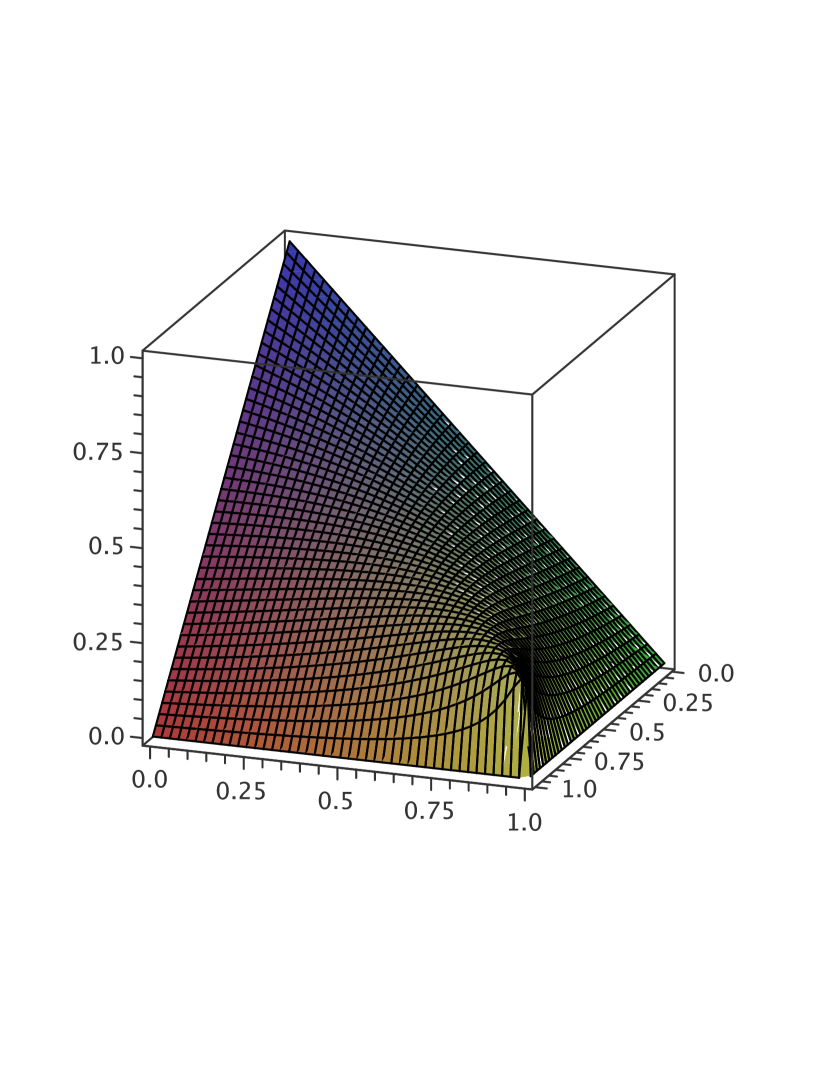
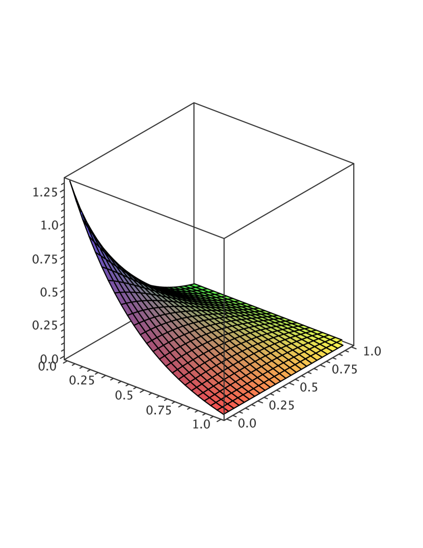
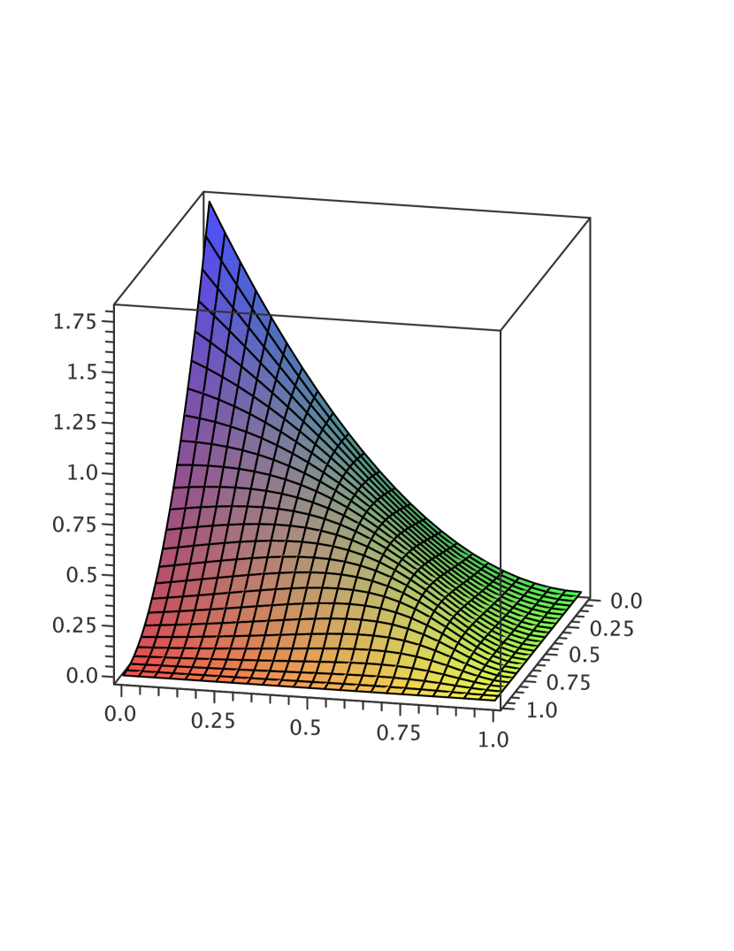
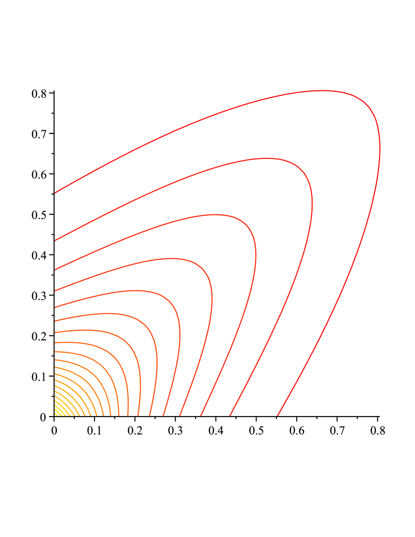
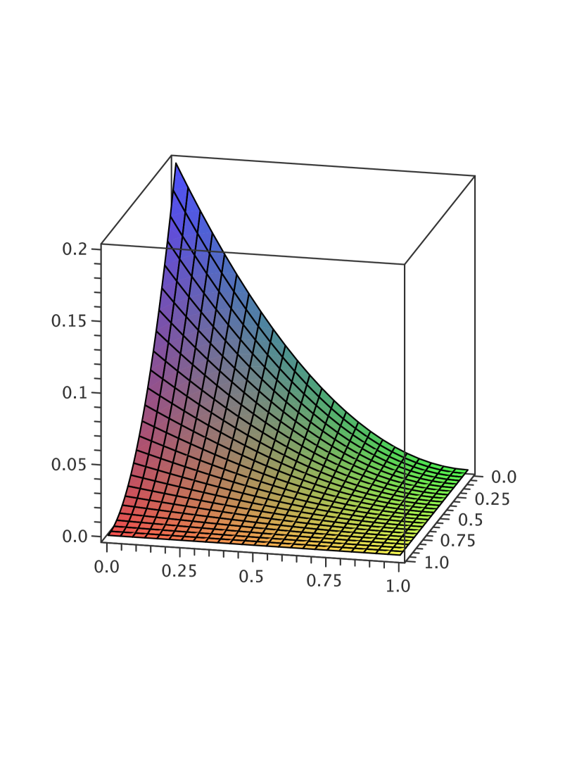
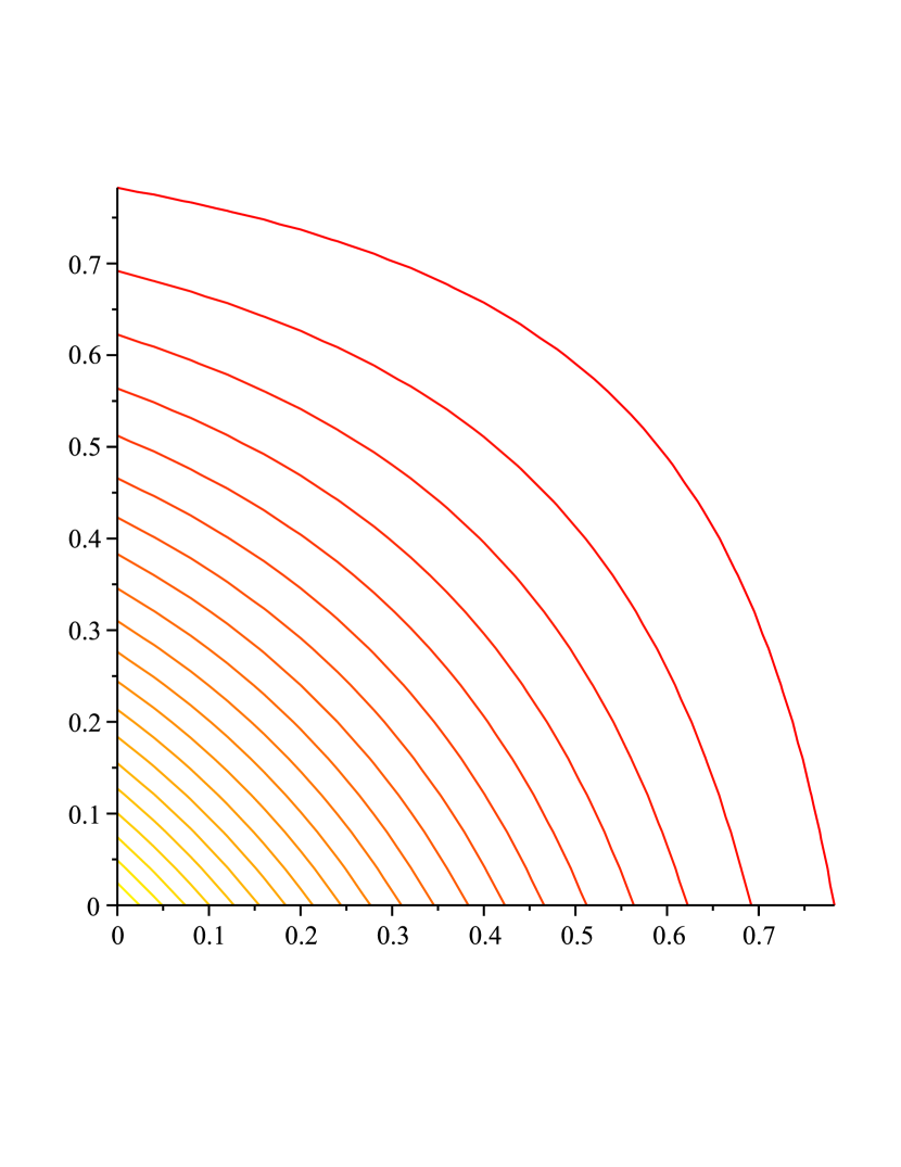
Figure 1: Plot and contour curves for the dependence hazard rate derivative
of a bivariate shared frailty model based on a standard exponential distribution over the range .
This choice of distributions results in a Clayton copula.
(c) The Frank copula is an Archimedean copula with generator
see Example 4.1.
For a bivariate survival function with the Frank copula as survival copula we obtain
as for univariate hazard rates with corresponding distribution functions .
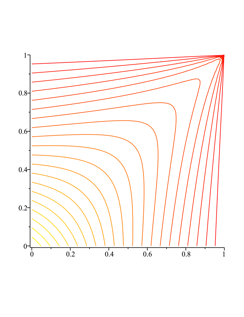
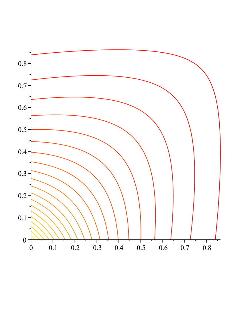
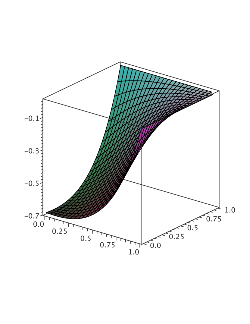
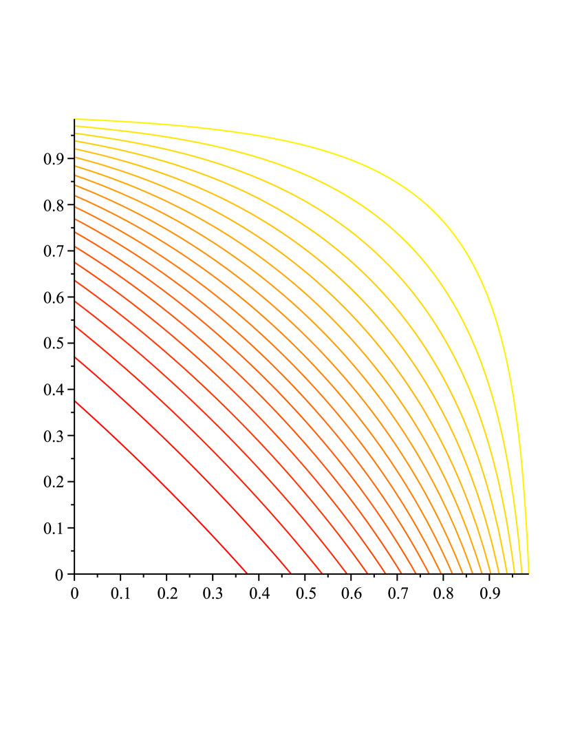
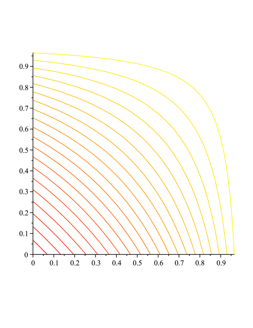
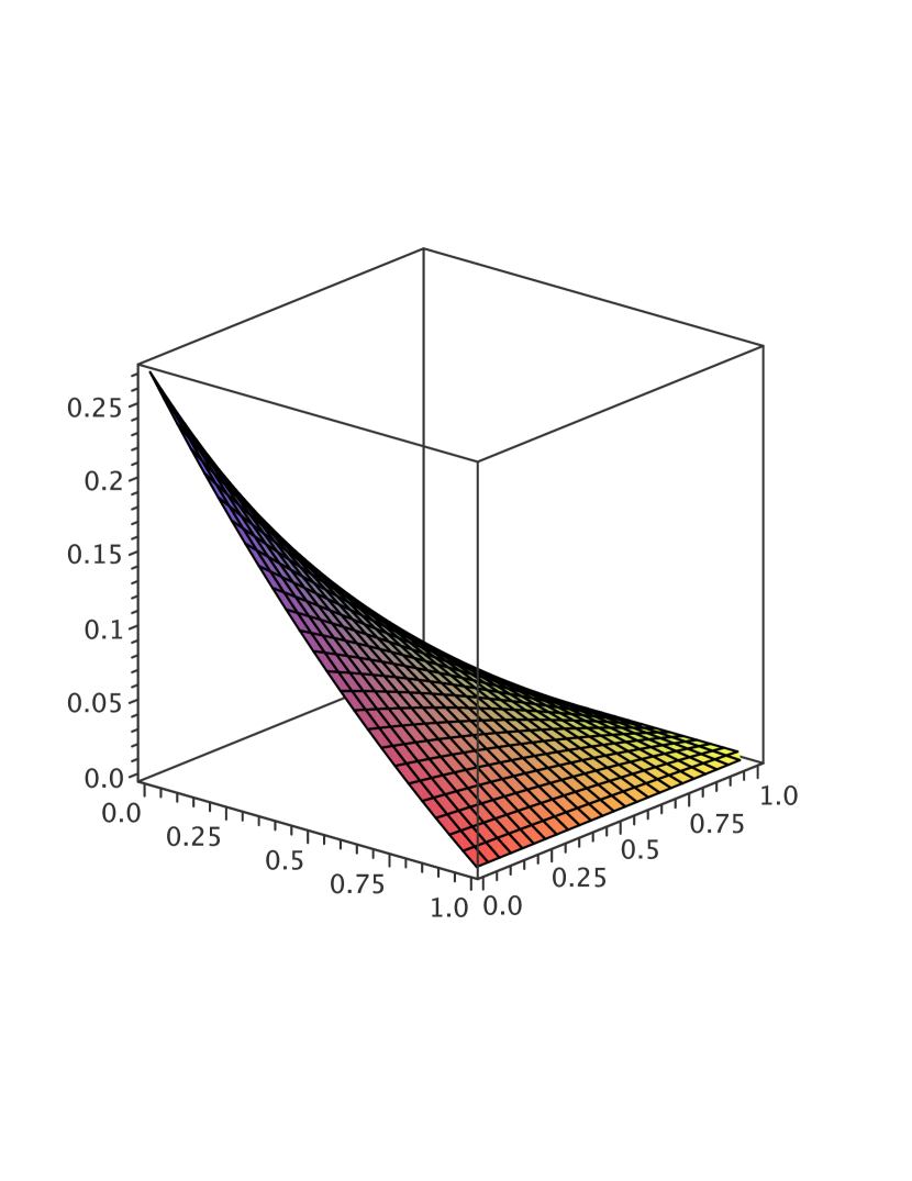
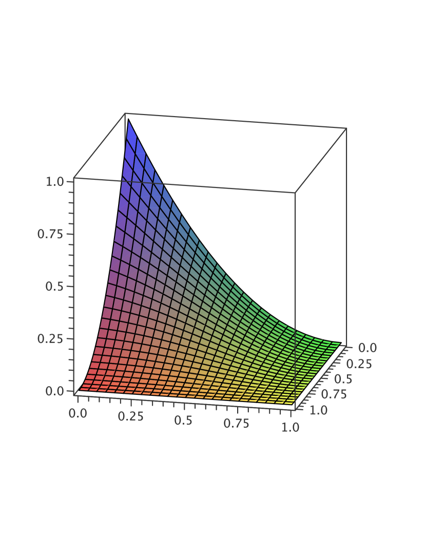
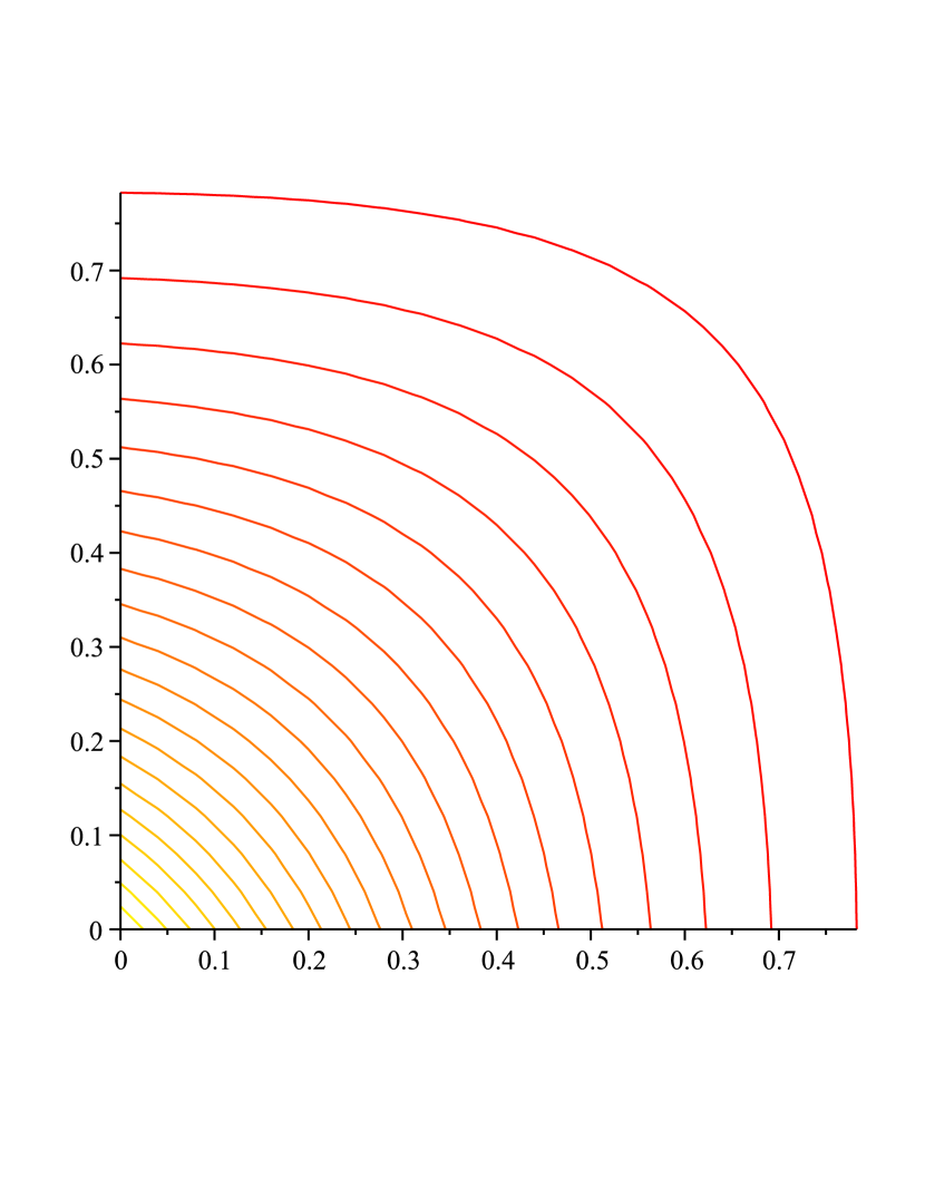
A visualization of is given in Figure 2.
(a)
(b)
(c)
(d)
Figure 2: Plots and contour curves for the dependence hazard rate derivative of a model with Frank copula as survival colula over the range , with different values of .
(d) Consider a shared frailty model based on an inverse Gaussian distribution, i.e.
where is normally distributed with and .
The Laplace transform of the frailty variable and the joint survival function of the shared frailty model are given by
and
, respectively.
We also see that
holds, so that this semiparametric dependence function is even invariant under different values of the parameter .
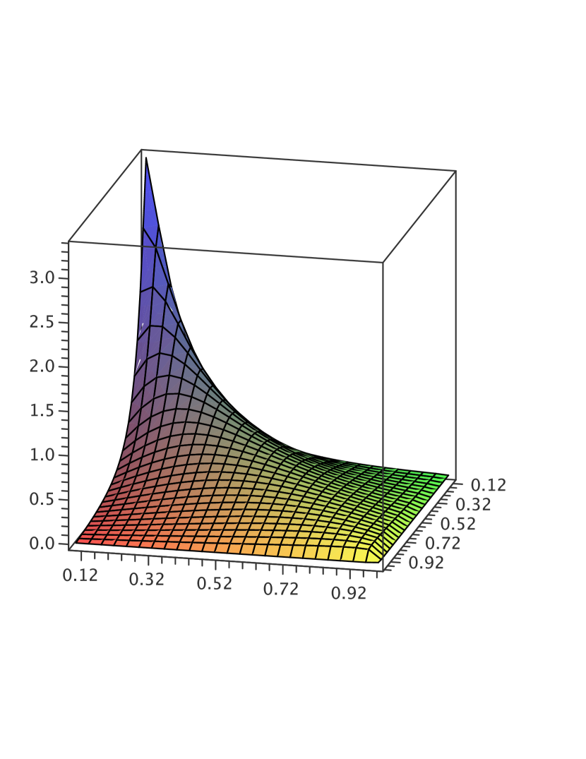
A visualization of is given in Figure 3.
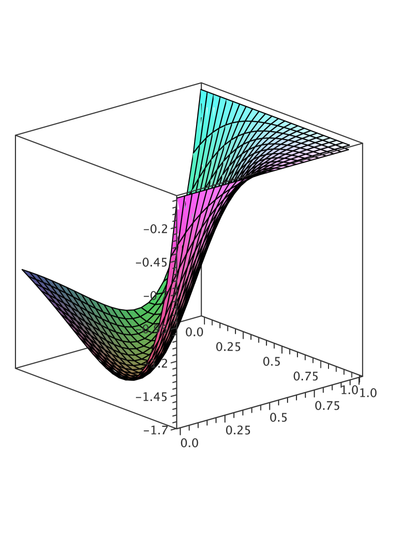
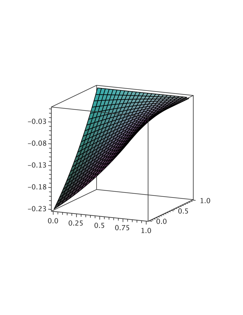
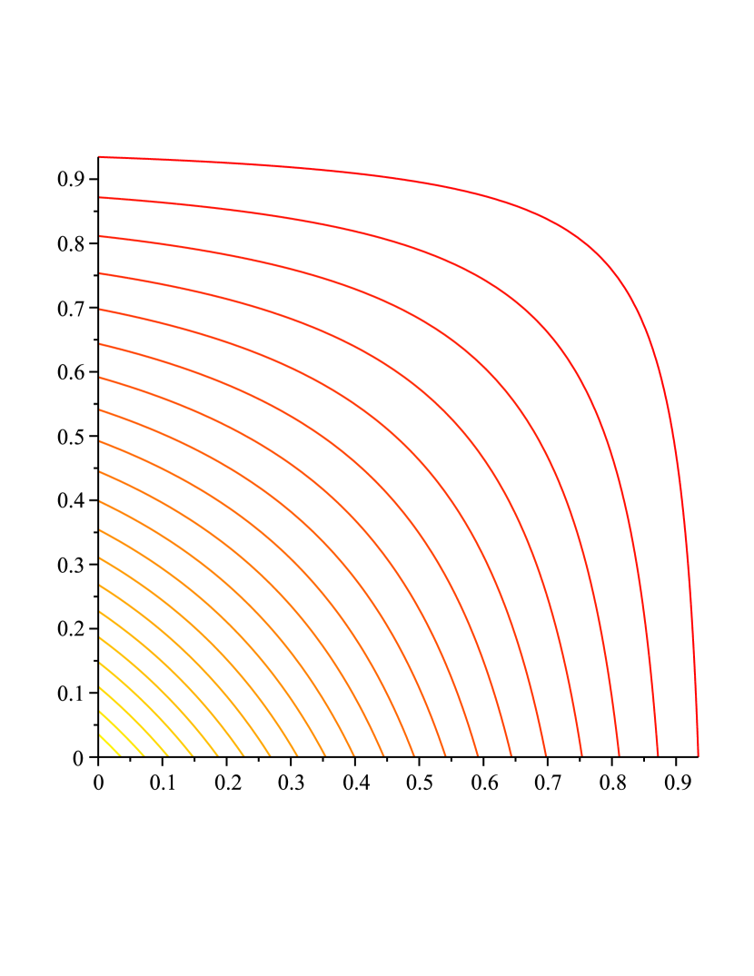
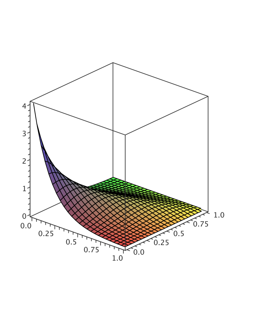
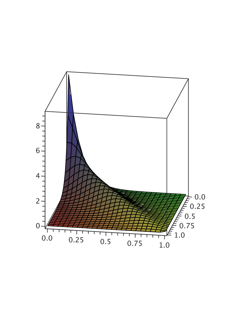
Figure 3: Plot and contour curves for the dependence hazard rate derivative
of a bivariate shared frailty model based on an inverse Gaussian distribution over the range .
Take note of the pole in the origin .
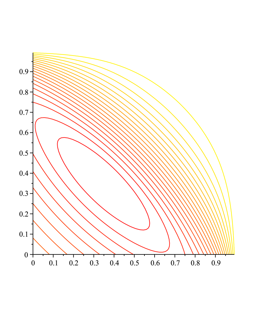
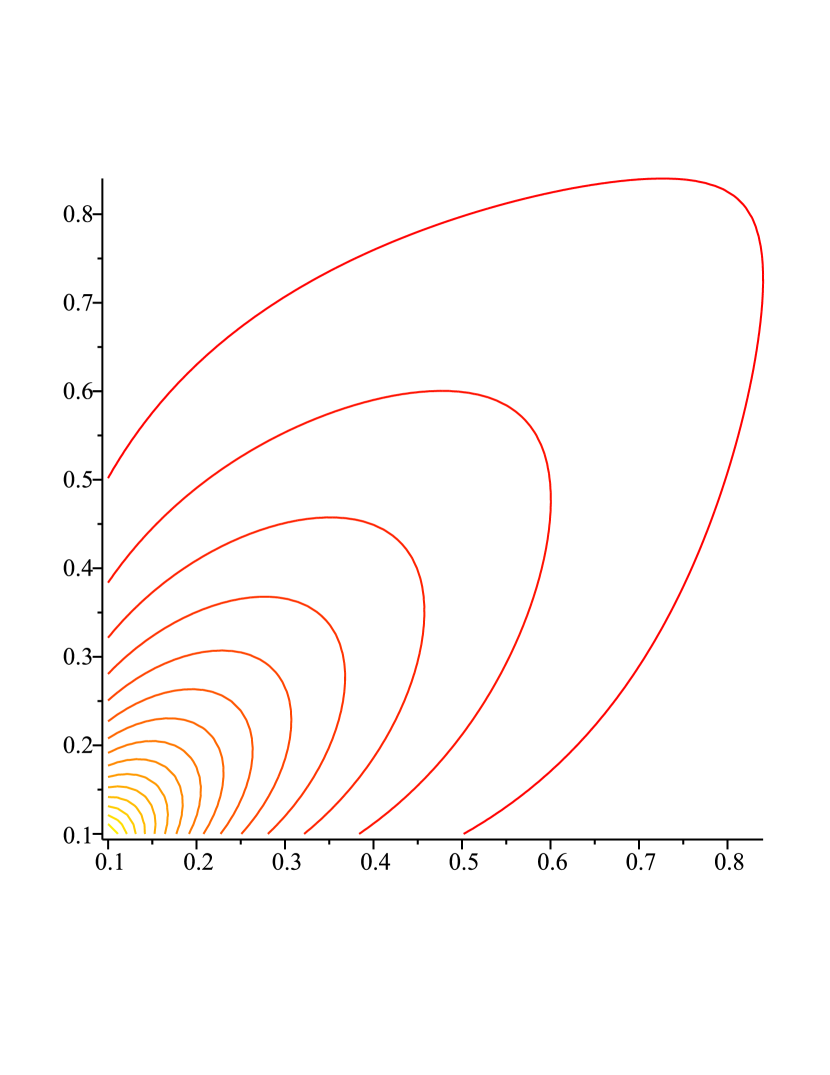
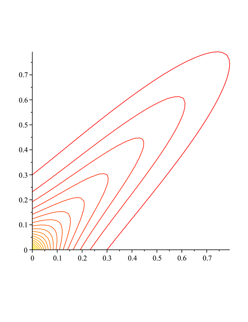
(e) For the correlated frailty model based on a -distribution as seen in Example 4.12 we have
Figure 4 shows a plot and a contour curve for with .
Note, that .
Comparing Figure 4 with Figure 8 in D,
we observe a high early dependence for all values of and an increased dependence along the diagonal
for higher values of .
(a)
(b)
Figure 4: Plot and contour curves for the dependence hazard rate derivative of a bivariate correlated frailty model
based on a bivariate chi-squared distribution over the range , with .
7 Copulas with higher degree of dependence: the hazard approach
In this section higher order exponent measures are studied in terms of hazard parameters.
We start with binary proportional dependence models which are developed in the spirit of Example 6.3.
Example 7.1.
The bivariate proportional dependence model can be extended for dimension .
Consider a family so that
holds for each .
Let be continuous univariate hazard measures on .
Then
defines the survival function of a -dimensional variable with proportional hazard dependence of the bivariate exponential measures
.
In Example 7.1 all higher dimensional exponent measures , , vanish.
To see that is indeed a survival function, assume (with no loss of generality) that
and consider the bivariate exponentially distributed random variable with survival function
where has the form (6.8) with parameter .
Introduce now a new -valued random variable with the coordinates at the position .
Let all other coordinates of be infinite .
Thus has the improper survival function
Consider now independent random variables for .
Then has the desired survival function .
Notice that this modeling of dependence can be generalized by linking arbitrary improper survival functions of the above kind.
This is again accomplished by applying the minimum operation to the corresponding random variables with values in .
In contrast to Example 7.1 survival models with trivial dependence measures
for all and are studied below.
Our apporach is based on statistical arguments used earlier for hazard-based score functions.
To this end, let be the uniform distribution on the interval with hazard measure .
Introduce the subset of those -dimensional, square-integrable functions in for which
holds for all . Functions of this kind serve as score functions for statistical models.
We start with the following useful observation.
Consider a copula which admits a -density .
Then the following conditions (1) and (2) are equivalent.
1.
All -dimensional marginals of the copula are independence copulas for .
2.
The function satisfies and .
In case of (1), (2) all exponent measures vanish for , .
Then the dependence part of reads as
which is studied below.
Recall that for the operator
is an isometry between Hilbert spaces; see Ritov and Wellner (1988) as well as Efron and Johnstone (1990).
Note that has an interpretation as hazard rate derivative for survival models.
We will now introduce a multivariate version of on .
Lemma 7.2.
For introduce the multivariate function
of .
We may then define
(7.1)
(a) The operator can be uniquely extended on
and
is an isometry between Hilbert spaces.
(b) Suppose that holds for some .
Then
(7.2)
holds for all .
Proof.
(a) The proof is mostly left to the reader and extends the bivariate calculus of Janssen and Rahnenführer (2002).
Let be an orthonormal basis of the Hilbert space .
Then product functions
form an orthonormal basis of .
We first introduce of these elements.
In the next step products of are considered as in (7.1)
and as well as can be extended by taking linear combinations of basis elements.
It is easy to see that is surjective.
If we add then is an orthonormal basis of and
including the index is an orthonormal basis of .
However, if one index is equal to zero then is orthogonal to .
All other elements of this kind are images of .
Thus is surjective.
(b) For formula (7.2) is proved in (3.8) of Janssen (1994).
Fubini’s theorem extends (7.2) to -dimensional product functions which are dense
in .
Since is an isometry, statement (7.2) holds in its general form.
∎
Theorem 7.3.
Suppose that (1) or (2) holds and let be the dependence part of the survival function
of the copula.
(a) Set for . The dependence part of is given by
(7.3)
(b) For each the function is
the density of a copula with survival function
.
The dependence part is given by
(7.4)
as with a uniform remainder on for .
Proof.
(a) Observe that holds.
If we divide by the marginals, then (7.2) yields the result.
(b) Observe that corresponds to the density of (7.3).
Taking the logarithm of (7.3) we obtain (7.4).
∎
Remark 7.4.
(a) Let be the
exponent representation of (7.4).
Up to the term the exponent is related to
.
(b) Note that
is the score function of the densities at .
These score functions can be used to obtain score tests for the null hypothesis of independence,
i.e. , against higher degree dependence.
Statistical aspects of hazard dependence models will be studied in a forthcoming work.
8 Discussion and conclusion
The present article considered the representation of dependent random variables in terms of dependence hazard measures
and the corresponding dependence parts of the joint survival function.
Furthermore, we have examined a useful representation of correlated frailty models
which led to the expression of higher-dimensional dependence hazard rates in terms of moments of an exponential family.
In particular, these rates are simply covariances of frailty variables for dimension 2.
It has also been shown that correlated frailty models are minimum-infinitely divisible iff its frailty vector is sum-infinitely divisible.
This equivalence yields an interesting one-to-one correspondence between the Lévy meausure of the frailty vector
and the exponent measure of the minimum-infinitely divisible correlated frailty model.
It follows that analytical properties of such Lévy measures might as well be examined in the context of extreme value theory.
Throughout the article we have made strong use of the copula concept
which enabled us to use arbitrary, continuous marginal distribution functions.
Here, the special shared frailty model had been shown to have a natural connection to Archimedean copulas.
Eventually, we have utilized this concept to analyze particularly interesting semiparametric quantities of dependence.
In the final chapter an isometry between Hilbert spaces exposed the relation of this semiparametric function to tangents in the space of square-integrable functions.
It is pointed out how score functions for dependence models can be transformed in terms of hazard dependence quantities.
Acknowledgements
This article has been developed at the Mathematical Institute of the University of Düsseldorf, Germany,
while this had been the permanent address of all three authors.
Appendix A Continuation and formulas of Example 4.12(a)
The joint survival function of at time is given by
where
denotes the determinant of
and
is the determinant of the covariance matrix
of and .
The marginal survival function of , , is given by
(a) is obvious since is uniquely determined by its two-dimensional marginals.
(b) By Lemma 4.6 (a) the vector
has independent components iff does.
Thus, the proof for (2) is trivial since the exponential function is a bijective mapping.
To prove (b) for (1) we introduce and we show
that is independent of iff is independent of for arbitrary indices .
Without loss of generality let and .
It is well known that, for a multivariate normally distributed vector ,
the random variables and are independent.
Now consider and repeatedly replace by
so that this covariance is expressed through expectations only depending on and .
The independence of these two random variables yields
Hence iff iff .
∎
Remark.
Let X be a correlated frailty model with frailty random vector W.
Then the survival function of X is minimum-infinitely disvisible
iff is sum-infinitely divisible.
Proof. Having the sum-infinite divisibility of ,
the minimum-infinite divisibility of is obvious:
this is a simple generalization of Lemma 4.10(b).
On the other hand, if is minimum-infinitely divisible,
then it is easy to see via induction that for all and
An application of a multivariate version of the Bernstein-Widder theorem (Theorem 1.3.1 of Zocher (2005))
now shows that is the Laplace transform of a probability measure on .
Hence, is the survival function of a -dimensional correlated frailty model.
Finally, another application of Lemma 4.10(b)
and the fact that each distribution determines a unique Laplace transform
show the sum-infinite divisibility of .
∎
Inserting the definition of and the Lévy-Khintchine formula yields
Hence, the proof for is covered by the following considerations for a general index set .
Note that, for fixed , the absoulte value of the function
is bounded by an -integrable function which is independent of :
for a constant , and this is integrable with respect to .
It follows that differentiation and integration are allowed to change places
and eventually the definition of concludes the proof via induction over .
∎
The proof for is a simpler version of the following proof; thus, it is left to the reader.
Applying Lemma 5.2 and Fubini’s theorem we get
The linearity of the integral and the definition of finish this proof.
∎
Appendix D Further Graphical Illustrations
(a)
(b)
(c)
(d)
Figure 5: Plots and contour curves for the dependence hazard rate derivative of a model with Frank copula as survival colula over the range , with different values of .
(a)
(b)
(c)
(d)
(e)
(f)
Figure 6: Plots and contour curves for the dependence hazard rate derivative of a model with Frank copula as survival colula over the range , with different values of .
Figure 7: Plot for the dependence hazard rate derivative in the proportional hazard rate dependence model (6.9)
for over the range .
(a)
(b)
(c)
(d)
Figure 8: Plots and contour curves for the dependence hazard rate derivative of a bivariate correlated frailty model
based on a bivariate chi-squared distribution over the range , with different values of .
Appendix E References
References
Aalen et al. (2008)
Aalen, O. O., Borgan, O., Gjessing, H. K., 2008. Survival and Event History
Analysis. Springer, New York.
Andersen et al. (1993)
Andersen, P. K., Borgan, O. B., Gill, R. T., Keiding, N., 1993. Statistical
models based on counting processes. Springer, New York.
Barndorff-Nielsen (1978)
Barndorff-Nielsen, O. E., 1978. Information and exponential families in
statistical theory. Wiley, Chichester.
Cox (1972)
Cox, D. R., 1972. Regression models and life-tables (with discussion). J. Roy.
Statist. Soc. B 34, 187–220.
Dabrowska (1996)
Dabrowska, D., 1996. Weak Convergence of a Product Integral
Dependence Measure. Scandinavian Journal of Statistics 23 (4).
Duchateau and Janssen (2008)
Duchateau, L., Janssen, P., 2008. The Frailty Model. Springer, New York.
Efron and Johnstone (1990)
Efron, B., Johnstone, I. M., 1990. Fisher’s information in terms of the hazard
rate. The Annals of Statistics 18, 38–62.
Genest and McKay (1986)
Genest, C., McKay, J., 1986. The joy of copulas: bivariate distributions with
uniform marginals. The American Statistician 40, 280–283.
Gill (1993a)
Gill, R., 1993a. Multivariate survival analysis, part 1. Theory of
Probability and its Applications 37 (1), 18–31.
Gill (1993b)
Gill, R., 1993b. Multivariate survival analysis, part 2. Theory of
Probability and its Applications 37 (2), 284–301.
Hartman and Wintner (1942)
Hartman, P., Wintner, A., 1942. On the infinitesimal generators of integral
convolutions. American Journal of Mathematics 64 (1), 273–298.
Hougaard (2000)
Hougaard, P., 2000. Analysis of multivariate survival data. Springer, New York.
Janssen (1985)
Janssen, A., 1985. One-sided stable distributions and the local approximation
of exponential families. 16th Eur. Meet. Statisticians, Marburg/Ger. 1984,
Suppl. Issues Stat. Decis. (2), 39–45.
Janssen (1994)
Janssen, A., 1994. On local odds and hazard rate models in survival analysis.
Statistics & Probability Letters 20 (5), 355–365.
Janssen and Rahnenführer (2002)
Janssen, A., Rahnenführer, J., 2002. A hazard-based approach to dependence
tests for bivariate censored models. Mathematical Methods of Statistics
11 (3), 297–322.
Joe (1997)
Joe, H., 1997. Multivariate models and dependence concepts. Chapman & Hall,
London.
Kimberling (1974)
Kimberling, C. H., 1974. A probabilistic interpretation of complete
monotonicity. Aequationes Mathematicae 10, 152–164.
Klein and Moeschberger (2003)
Klein, J. P., Moeschberger, M. L., 2003. Survival Analysis: Techniques for
Censored and Truncated Data, 2nd Edition. Springer, New York.
Marshall and Olkin (1988)
Marshall, A., Olkin, I., 1988. Families of multivariate distribution. Journal
of the American Statistical Association 83, 834–841.
McNeil and Nes̆lehová (2009)
McNeil, A. J., Nes̆lehová, J., 2009. Multivariate Archimedean copulas,
-monotone functions and -norm symmetric distributions. The Annals
of Statistics 37 (5B), 3059–3097.
Meerschaert and Scheffler (2001)
Meerschaert, M. M., Scheffler, H.-P., 2001. Limit distributions for sums of
independent random vectors: Heavy tails in theory and practice. John Wiley &
Sons.
Nelsen (2006)
Nelsen, R. B., 2006. An introduction to copulas, 2nd Edition. Springer, New
York.
Oakes (1989)
Oakes, D., 1989. Bivariate survival models induced by frailties. Journal of the
American Statistical Association 84 (406), 487–493.
Okhrin et al. (2013)
Okhrin, O., Okhrin, Y., Schmid, W., 2013. Properties of hierarchical
Archimedean copulas. Statistics & Risk Modeling 30, 21–53.
Petrov (1995)
Petrov, V. V., 1995. Limit theorems of probability theory: sequences of
independent random variables. Oxford University Press, Oxford.
Resnick (1987)
Resnick, S. I., 1987. Information and exponential families in statistical
theory. Applied Probability, Springer, New York.
Ritov and Wellner (1988)
Ritov, Y., Wellner, J. A., 1988. Censoring, martingales, and the Cox model.
Contemporary Mathematics 80, 191–219.
Sklar (1959)
Sklar, A., 1959. Fonctions de répartition à n dimensions et leurs
marges. Publications de l’Institut de Statistique de l’Université de Paris
8 (3), 229–231.
Völker (2010)
Völker, D., 2010. Modeling dependencies in insurance using multi-frailty
models: r-frailty copulas. Preprint.
Wienke (2011)
Wienke, A., 2011. Frailty models in survival analysis. Chapman and Hall/CRC,
Boca Raton, Florida.
Zocher (2005)
Zocher, M., 2005. Multivariate mixed poisson processes. Dissertation,
Technische Universität Dresden.