Quantum Fisher information of fermionic cavity modes in an accelerated motion

Abstract

We investigate the effect of the inertial and non-inertial segments of relativistic motion on the quantum Fisher information of $\left(1+1\right)$ Dirac field modes confined to cavities. For the purpose we consider $\theta$ parameterized two-qubit pure entangled state. In this setting, the initial state is obtained by a unitary operation which entangles the two confined modes of cavities of Alice and Bob. In the situation that Rob’s cavity, initially inertial, accelerates uniformly with respect to its proper time and then again becomes inertial while Alice’s cavity remains inertial, we analyze the quantum Fisher information of the system. First of all, we find that the quantum Fisher information of the pure composite system $\mathcal{F}_{\theta}$ with respect to parameter $\theta$ is invariant regardless of the non-inertial movement. However in the quantum Fisher information distribution over the subsystems of Alice’s and Rob’s cavities, the quantum Fisher information over the Rob’s cavity is shown to be the periodic degradation behavior depending upon the parameter $\theta$. In order to check whether the invariance of the quantum Fisher information of the composite system is an intrinsic property, we consider a depolarizing state of the pure composite system. Then we show that the quantum Fisher information of the Werner state with respect to parameter $\theta$ is not invariant. Furthermore for the non-inertial motion of a single cavity, we find that the quantum Fisher information with respect to parameter $\theta$ for a $\theta$ parameterized initial state is degraded in terms of acceleration. Finally subadditivity of the quantum Fisher information is shown regardless of the pure composite system or the Werner state.

I Introduction

Recently quantum Fisher information (QFI) Braunstein1996135 ; PhysRevLett.72.3439 ; 1976quantum has gained considerable attention as a promising candidate to understand the information contents of quantum states. It is well known that QFI has been successfully applied to quantum statistical inference and estimation theory PhysRevLett.91.180403 ; PhysRevA.84.042121 . When information is encrypted in a set of quantum states, more often in terms of appropriate parameters, extraction of the encoded information requires the distinction between different quantum states. This requirement can be accomplished through measurements that yield a set of observations characterized by those parameters. Therefore the problem of distinguishing the quantum states is transformed into a problem of parameter estimation.
The classical Fisher information is known to provide the lower bound on the variance of the parameter estimation in terms of the well known Crame$\acute{}$r-Rao bound. For asymptotically large sets of observations, the maximum likelihood estimation (MLE) approach provides unbiased parameter estimation that can attain this bound Fisher1925 . However, when one should deal with quantum information, since quantum information content is much more complex and intrinsically contains non-trivial characteristics that can not be associated with their classical counterpart Braunstein1996135 ; holevo2011probabilistic , the quantum Fisher information should be coined 1976quantum ; holevo2011probabilistic ; PhysRevLett.72.3439 as a natural extension to the classical Fisher information.

Furthermore, successful efforts to combine relativity and quantum information theory have opened new avenues to explain quantum behavior at a macroscopic scale PhysRevD.14.2460 ; PhysRevD.14.870 ; Wald94quantumfield ; fabbri2005modeling ; RevModPhys.76.93 . A focus of this area of research is the dynamics of information contents under the Unhruh-Hawking effect AlcingObDEpEnt-0264-9381-29-22-224001 ; PhysRevA.82.042332 ; RevModPhys.80.787 . For example, the dynamics of entanglement PhysRevLett.95.120404 ; PhysRevD.85.061701 ; PhysRevA.87.022338 ; PhysRevD.85.025012 ; PhysRevA.74.032326 , quantum discord PhysRevA.80.052304 ; PhysRevA.81.052120 ; PhysRevA.86.032108 , and fidelity of teleportation PhysRevLett.91.180404 ; PhysRevLett.110.113602 have already been studied. For instance, the correlations induced by maximally entangled bosonic or fermionic bipartite states were found to be degraded due to the accelerated motion of one party with respect to the other inertial party PhysRevD.85.061701 ; PhysRevD.85.025012 .
The study of Unruh-Hawking effect on the quantum Fisher information is a crucial step to use QFI as a reliable resource for quantum metrology in a relativistic regime. Aspachs et al. described the optimal detection process of Unruh-Hawking effect itself and showed that the Fock states can achieve maximal QFI with a scalar field in a two-dimensional Minkowski spacetime PhysRevLett.105.151301 . In Yao2014 authors investigated the performance of QFI for both scalar and Dirac fields parameterized by weight and phase parameters in non-inertial frames. In MehdiAhmadi2013 ; PhysRevD.89.065028 , the authors evaluated the QFI of the acceleration parameter for the relativistic scalar and Bosonic quantum fields confined to a cavity using Bures Statistical distance BuresMR0236719 .

The main contribution of this paper is to investigate QFI under the influence of non-uniform motion, on the precision of parameter estimation for the parameter $\theta$. The parameter $\theta$ is encoded through a unitary operation, which causes the two-qubit entangled state of the Dirac fields confined in two cavities. In other words, the entangling power of a unitary operation is precisely unknown, and the parameter $\theta$ arises naturally. Although, the evaluation of QFI for various physical parameters in the inertial frames is equally important and has been studied recently in different scenarios, in this manuscript the QFI dynamics is investigated in the perspective of non-uniform motion.

More precisely, we follow the Dirac field analysis proposed in [19], where the modes of massless Dirac field are confined to the two cavities with Dirichlet’s boundary conditions and one of the cavities remains inertial while the other cavity undergoes the segments of inertial and non-inertial motion with uniform acceleration. We restrict the uniform acceleration to be very small $\left(a\ll 1\right)$ and use perturbation theory to observe the variation of the QFI for the confined modes of the Dirac field with respect to the parameter $\theta$, under the accelerated motion.

The rest of the paper is organized as follows. In Sec. II, we briefly review the properties of QFI and discuss the recent developments regarding its analytic evaluation. The perturbed Bogoliubov coefficients and Fock space quantization for vacuum and one charged particle fermionic states in the cavities are described in Sec. III. The QFI for two mode fermionic Fock state shared between Alice’s and Rob’s cavities and distribution of QFI over each cavity is discussed in Sec. IV. And the behavior of QFI for parameterized initial state in a single cavity under the non-initial motion is studied. In Sec. V, we extend our investigation to Werner state PhysRevA.40.4277 . In Sec. VI, we conclude and discuss our results.

II Quantum Fisher Information

Consider a quantum state $\rho_{\lambda}$ having a one parameter family of N-dimensional quantum states, with parameter $\lambda$. A set of quantum measurements $\{E\left(\xi\right)\}$, which is POVM, should be performed on $\rho_{\lambda}$ to extract the information about unknown parameter $\lambda$. This process resembles the classical case where the parameter estimation is performed from the observed data obtained from classical experiments and the efficiency of the estimate(s) is measured in terms of the classical Fisher information 1976quantum ; Fisher1925 ; holevo2011probabilistic

$$F_{\lambda}=\int d\xi p\left(\xi|\lambda\right)\left[\partial_{\lambda}\ln p\left(\xi|\lambda\right)\right]^{2}=\int d\xi\frac{\left(\partial_{\lambda}p\left(\xi|\lambda\right)\right)^{2}}{p\left(\xi|\lambda\right)},$$ (1)

where $p\left(\xi|\lambda\right)$ denotes the conditional probability of observing the result $\xi$ provided the value of the parameter is $\lambda$. However, the quantum Fisher information differs significantly in the operational sense due the fact that the probability $p\left(\xi|\lambda\right)$ results from measurement by the quantum operator $E\left(\xi\right)$ rather than a mere classical experiment. According to Born’s rule, $p\left(\xi|\lambda\right)=Tr\left[E\left(\xi\right)\rho_{\lambda}\right]$ represents the conditional probability of obtaining the outcome $\xi$ when the given value of the parameter is $\lambda$. In the quantum world, the parameter estimation problem can be thought of as the problem of searching for the set of measurements $\{E\left(\xi\right)\}$ that yields the optimal value of (1). Therefore, the quantum Fisher information can be defined as Braunstein1996135 ; PhysRevLett.72.3439

$$\mathcal{F}_{\lambda}=\max_{E\left(\xi\right)}F_{\lambda}.$$ (2)

Further, using the notion of symmetric logarithmic derivative (SLD) introduced in 1976quantum

$$\partial_{\lambda}\rho_{\lambda}=\frac{1}{2}\left(\rho_{\lambda}L_{\lambda}+L_{\lambda}\rho_{\lambda}\right),$$ (3)

we obtain an alternate expression for the QFI as

$$\mathcal{F}_{\lambda}=Tr\left(\rho_{\lambda}L_{\lambda}^{2}\right)=Tr\left(\partial_{\lambda}\rho_{\lambda}L_{\lambda}\right),$$ (4)

where the operator $L_{\lambda}$ is the solution of the Lyapunov matrix equation PARIS2009 given by Eq. (3). It is worth noticing that expressions of QFI in (2) and (4) are equivalent in the sense that the operator $L_{\lambda}$ admits the spectral decomposition in the same basis as used for the spectral decomposition of $\rho_{\lambda}$. Therefore, based on the spectral decomposition $\rho_{\lambda}=\sum_{i=1}^{N}p_{i}|\psi_{i}\times\psi_{i}|$, the operator $L_{\lambda}$ is written as PARIS2009

$$L_{\lambda}=2\sum_{m,n}^{N}\frac{\left|<\psi_{m}\left|\partial_{\lambda}\rho_{\lambda}\right|\psi_{n}>\right|}{p_{m}+p_{n}}\left|\psi_{m}\times\psi_{n}\right|,$$ (5)

where the eigenvalues $p_{i}\geq 0$ and $\sum_{i=1}^{N}p_{i}=1$. In turn, the set of eigenvectors of $L_{\lambda}$ provides the optimal POVM to obtain the QFI. Making use of (4) and (5), the QFI can be rewritten as PARIS2009

$$\mathcal{F}_{\lambda}=2\sum_{m,n}^{N}\frac{\left|<\psi_{m}\left|\partial_{\lambda}\rho_{\lambda}\right|\psi_{n}>\right|^{2}}{p_{m}+p_{n}}.$$ (6)

Using the completeness relation

$$\sum_{i=M+1}^{N}|\psi_{i}\times\psi_{i}|=\mathbb{I}-\sum_{i=1}^{M}|\psi_{i}\times\psi_{i}|,$$ (7)

where M denotes the number of eigenvectors corresponding to non-zero eigenvalues and represents the dimension of the support of $\rho_{\lambda}$, Zhang et al. provided a relatively simple expression to evaluate the QFI for general states as PhysRevA.88.043832

$$\mathcal{F}_{\lambda}=\!\!\sum_{i=1}^{M}\frac{\left(\partial_{\lambda}p_{i}\right)^{2}}{p_{i}}+\!\!\sum_{i=1}^{M}4p_{i}\mathcal{F}_{\lambda,i}-\!\!\sum_{i\neq j}^{M}\frac{8p_{i}p_{j}\left|\big{<}\psi_{i}|\partial_{\lambda}\psi_{j}\big{>}\right|^{2}}{p_{i}+p_{j}},$$ (8)

where $\mathcal{F}_{\lambda,i}$ is the QFI of the pure state $|\psi_{i}>$ given by

$$\mathcal{F}_{\lambda,i}=\big{<}\partial_{\lambda}\psi_{i}|\partial_{\lambda}\psi_{i}\big{>}-\left|\big{<}\psi_{i}|\partial_{\lambda}\psi_{i}\big{>}\right|^{2}.$$ (9)

It is noteworthy that the QFI of a low rank density matrix is now only determined by its support spanned by the eigenvectors, $|\psi_{i}\big{>};\quad i=1,\cdots,M$, corresponds to nonzero eigenvalues. In fact, the first term on the right hand side of (8) represents the classical case where the set of nonzero eigenvalues behaves like a classical probability distribution. And the second contribution of (8) denotes the weighted average of QFI due to all the pure-states. The last term of (8) captures the QFI from the mixture of pure states and therefore causes the decrease in the total QFI. Therefore, the last two terms can be interpreted as the quantum part of the Fisher information while the first term represents its classical constituent. In this paper, we will exploit Eq. (8) due to its relative simplicity and clear physical interpretation to find the QFI for the modes of the Dirac field confined to the inertial and non-inertial cavities.

III Bogoliubov Transformation For Inertial and Non-inertial Segments

In order to find the unitary transformation of cavity’s transitions between the inertial and non-inertial segments of motion, we setup two cavities with the observers referred to as Alice and Rob, respectively. Both the cavities are inertial and completely overlap at $t=0$. Here we assume that the cavity walls are placed at $x=a$ and $x=b$ where $0<a<b$. Rob’s cavity then moves with uniform acceleration to the right along the time-like killing vector $\partial_{\eta}$ for duration $\eta=0$ to $\eta=\eta_{1}$ in the Rindler co-ordinates. Duration of the acceleration, $\frac{2}{a+b}$, with respect to proper time measured at the center of the cavity is thus $\tau_{1}=\frac{a+b}{2}\eta_{1}$. Finally, Rob’s cavity again becomes inertial with respect to its rest frame. The Alice’s cavity remains inertial throughout this trip of Rob’s cavity. Therefore, three segments of Rob’s trajectories can be identified as Regions I, II and III.
This grafting process of cavity motion is explained here to make this paper sufficiently self contained. Earlier the same process is introduced and exploited by ARLEEPHDThesis ; PhysRevD.85.025012 to study the dynamics of the entanglement for bosonic and fermionic cavities.
The Dirac field representation in three regions is

$$\textup{I:}\quad\psi = \sum_{n\geq 0}a_{n}\psi_{n}+\sum_{n<0}b_{n}^{\dagger}\psi_{n},$$ (10a)

$$\textup{II:}\quad\psi = \sum_{n\geq 0}\hat{a}_{n}\hat{\psi}_{n}+\sum_{n<0}\hat{b}_{n}^{\dagger}\hat{\psi}_{n},$$ (10b)

$$\textup{III:}\quad\psi = \sum_{n\geq 0}\tilde{a}_{n}\tilde{\psi}_{n}+\sum_{n<0}\tilde{b}_{n}^{\dagger}\tilde{\psi}_{n},$$ (10c)

with the respective non vanishing anticommutators

$$\textup{I:}\quad\{a_{m},a_{n}^{\dagger}\} = \{b_{m},b_{n}^{\dagger}\}=\delta_{mn},$$ (11a)

$$\textup{II:}\quad\{\hat{a}_{m},\hat{a}_{n}^{\dagger}\} = \{\hat{b}_{m},\hat{b}_{n}^{\dagger}\}=\delta_{mn},$$ (11b)

$$\textup{III:}\quad\{\tilde{a}_{m},\tilde{a}_{n}^{\dagger}\} = \{\tilde{b}_{m},\tilde{b}_{n}^{\dagger}\}=\delta_{mn}.$$ (11c)

Using Bogoliubov transformation, the Dirac field modes between Region I and II are related as PhysRevD.85.025012

$$\hat{\psi}_{m}=\sum_{n}A_{mn}\psi_{n},$$ (12)

where ${\psi}_{n}$ and $\hat{\psi}_{m}$ are the Dirac field modes in regions I and II respectively. For the small acceleration case, Friis et al. PhysRevD.85.025012 derived these coefficients $A_{mn}$ in the perturbative regime by introducing the dimensionless parameter $h=\frac{2L}{a+b}$, satisfying $0<h<2$. These coefficients preserve the unitarity of the transformation to the order $O\left(h^{2}\right)$ for $s>0,s\rightarrow 0_{+}$ and are given in terms of Maclaurin’s series expansion as PhysRevD.85.025012 ; ARLEEPHDThesis

$$A_{mn}=A_{mn}^{\left(0\right)}+A_{mn}^{\left(1\right)}+A_{mn}^{\left(2\right)}+O(h^{3}),$$ (13)

where the superscripts indicate the power of parameter $h$. During the non-inertial trajectory, modes $\hat{\psi}_{m}$ in Rob’s cavity remain independent and do not interact. Hence, these modes can only develop some phases during the non-inertial duration $0\leq\eta\leq\eta_{1}$. This change in the modes can be balanced by introducing a diagonal matrix $G\left(\eta_{1}\right)$ whose diagonal entries are PhysRevD.85.025012

$$G_{nn}\left(\eta_{1}\right)=\exp\left(i\Omega_{n}\eta_{1}\right).$$ (14)

For $\eta\geq\eta_{1}$, the transformation from region II to region III can be obtained by simply using the inverse transformation $A^{\dagger}=A^{-1}$. The evolution of the Dirac field mode from region I to region III in Rob’s cavity can then be expressed by the Bogoliubov transformation matrix

$$\mathcal{A}=A^{\dagger}G\left(\eta_{1}\right)A.$$ (15)

Thus the Bogoliubov transformation for the Dirac field modes between regions I and III reads

$$\tilde{\psi}_{m}=\sum_{n}\mathcal{A}_{mn}\psi_{n}.$$ (16)

It can be noticed that $\mathcal{A}$, being the composition of unitary matrices, is also a unitary matrix to the order $h^{2}$. Similarly, the Bogoliubov transformation for the Dirac field mode operators can also be expressed as ARLEEPHDThesis ; PhysRevD.85.025012

$$k>0:\qquad a_{k} = \sum_{l\geq 0}\tilde{a}_{l}\mathcal{A}_{lk}+\sum_{l<0}\tilde{b}_{l}^{\dagger}\mathcal{A}_{lk},$$ (17a)

$$k<0:\qquad b_{k} = \sum_{l\geq 0}\tilde{a}_{l}^{\dagger}\mathcal{A}_{lk}+\sum_{l<0}\tilde{b}_{l}\mathcal{A}_{lk}.$$ (17b)

The relation between the Fock vacua in regions I and III denoted by $|0\big{>}$ and $|\tilde{0}\big{>}$ is fabbri2005modeling ; PhysRevD.85.025012

$$|0\big{>}=Ne^{W}|\tilde{0}\big{>},$$ (18)

where

$$W=\sum_{p\geq 0,q<0}V_{pq}\tilde{a}_{p}^{\dagger}\tilde{b}_{q}^{\dagger}.$$ (19)

The coefficient matrix $V$ and the normalization constant $N$ are the unknowns to be evaluated. Using (10a),(10c), and (16), the coefficient matrix is given by

$$V=V^{(0)}+V^{(1)}+O(h^{2})=V^{(1)}+O(h^{2}),$$ (20)

with

$$V^{(1)}_{pq}=\mathcal{A}_{pq}^{(1)*}G_{q}=-\mathcal{A}_{qp}^{(1)}G_{p}^{*}$$ (21)

The relation between Fock vacua in regions I and III given by (18) yields ARLEEPHDThesis ; PhysRevD.85.025012

$$\big{|}0\big{>}=\bigl{(}1-\frac{1}{2}\sum_{p\geq 0,q<0}|V_{pq}|^{2}\bigr{)}|\tilde{0}\big{>}+\sum_{p,q}V_{pq}|\tilde{1}_{p}\big{>}^{+}|\tilde{1}_{q}\big{>}^{-}-\frac{1}{2}\sum_{p,q}\sum_{i,j}V_{pq}V_{ij}\phi_{p,i}\phi_{q,j}|\tilde{1}_{p}\big{>}^{+}|\tilde{1}_{i}\big{>}^{+}|\tilde{1}_{q}\big{>}^{-}|\tilde{1}_{j}\big{>}^{-}\!\!+O(h^{3}).$$ (22)

where $|\tilde{1}_{p}\big{>}^{+}:=\tilde{a}_{p}^{\dagger}|\tilde{0}\big{>}^{+}$ and $|\tilde{1}_{q}\big{>}^{-}:=\tilde{b}_{q}^{\dagger}|\tilde{0}\big{>}^{-}$ represent the single-particle Fock states for modes $p\geq 0$ and $q<0$, respectively. The sign $\pm$ in the superscript denotes the sign of the charge. Further, the term $\phi_{pi}:=1-\delta_{p,i}$ is introduced to incorporate the Pauli-exclusion principle for the single particle states with same charge sign. Also the ordering of the single-particle kets corresponds to the ordering of the fermionic creation operators rather than the fermionic modes ARLEEPHDThesis . Similarly, the charged single particle states in region III are ARLEEPHDThesis ; PhysRevD.85.025012

$$k>0:\quad|1_{k}\big{>}^{+}= -\sum_{p,q}V_{pq}\mathcal{A}_{qk}^{*}|\tilde{1}_{p}\big{>}^{+}+\sum_{m\geq 0}\mathcal{A}_{mk}^{*}\bigl{\{}\bigl{(}1-\frac{1}{2}\sum_{p,q}|V_{pq}|^{2}\bigr{)}|\tilde{1}_{m}\big{>}^{+}+\sum_{p,q}V_{pq}\phi_{pm}|\tilde{1}_{m}\big{>}^{+}|\tilde{1}_{p}\big{>}^{+}|\tilde{1}_{q}\big{>}^{-}$$

$$-\frac{1}{2}\sum_{p,q;i,j}V_{pq}V_{ij}\phi_{pi}\phi_{pm}\phi_{mi}\phi_{qj}|\tilde{1}_{m}\big{>}^{+}|\tilde{1}_{p}\big{>}^{+}|\tilde{1}_{i}\big{>}^{+}|\tilde{1}_{q}\big{>}^{-}|\tilde{1}_{j}\big{>}^{-}\bigr{\}}+O(h^{3}),$$ (23a)

$$k<0:\quad|1_{k}\big{>}^{-}= \sum_{p,q}V_{pq}\mathcal{A}_{pk}|\tilde{1}_{q}\big{>}^{-}+\sum_{m<0}\mathcal{A}_{mk}\bigl{\{}\bigl{(}1-\frac{1}{2}\sum_{p,q}|V_{pq}|^{2}\bigr{)}|\tilde{1}_{m}\big{>}^{-}+\sum_{p,q}V_{pq}\phi_{qm}|\tilde{1}_{p}\big{>}^{+}|\tilde{1}_{q}\big{>}^{-}|\tilde{1}_{m}\big{>}^{-}$$

$$-\frac{1}{2}\sum_{p,q;i,j}V_{pq}V_{ij}\phi_{pi}\phi_{qm}\phi_{qj}\phi_{mj}|\tilde{1}_{p}\big{>}^{+}|\tilde{1}_{i}\big{>}^{+}|\tilde{1}_{q}\big{>}^{-}|\tilde{1}_{j}\big{>}^{-}|\tilde{1}_{m}\big{>}^{-}\bigr{\}}+O(h^{3}),$$ (23b)

where the one particle states $|1_{k}\big{>}^{\pm}$ in region I are

$$k\geq 0:\qquad|1_{k}\big{>}^{+} = a_{k}^{\dagger}|0\big{>},$$ (24a)

$$k<0:\qquad|1_{k}\big{>}^{-} = b_{k}^{\dagger}|0\big{>}.$$ (24b)

IV Quantum Fisher Information for two-mode states

Here we investigate the behavior of the QFI for a complete trip of a two mode entangled states from region I to region III in the perturbative regime to the order $h^{2}$ and study how the uniform acceleration affects the QFI of the evolved fermionic modes confined to the cavities. Although a single cavity can reveal the effect of non-inrtial (accelerated) motion in time, as described in PhysRevD.85.061701 and PhysRevD.85.025012 , the entangled mode in two cavities where one cavity remains inertial throughout while the other may have segments of inertial and non-inertial motion may show richer effect of non-inrtial (accelerated) motion. And a localization of non-uniform (accelerated) motion in time can then be achieved by considering the initial and final segments of the accelerated cavity to be inertial PhysRevD.85.025012 . We therefore employed and followed the argument proposed by PhysRevD.85.061701 and PhysRevD.85.025012 to consider the effects of non-uniform motion on the precision of parameter estimation. In addition, we have also considered a single cavity scenario for QFI analysis as an extension.

IV.1 Evaluation of Perturbed Eigenvalues and Eigenvectors

We consider a bipartite two qubit pure state parameterized by parameter $\theta$ in region I. The state consists of two Dirac field modes where one of the modes is confined to Alice’s cavity and the other is confined to Rob’s cavity. The initial parameterized state is

$$\big{|}\psi^{\pm}_{init}\big{>}_{\nu}=\cos\theta\big{|}0\big{>}_{A}\big{|}0\big{>}_{R}\pm\sin\theta\big{|}1_{m}\big{>}_{A}^{\mu}\big{|}1_{k}\big{>}_{R}^{\nu},$$ (25)

where the subscripts A and R refer to the cavity of Alice and Bob, respectively. In this setting, the initial state can be obtained by a unitary operation which entangles the two confined modes of cavities of Alice and Bob. However the rate of entanglement, which is controlled by the parameter $\theta$, is unknown. In other words, the parameter $\theta$ indicates the initial entanglement of the two confined modes, and is not known in advance. However, the initially chosen entangled state may provide some prior knowledge about the range of the parameter but not the actual value. The superscripts $\mu$ and $\nu$ indicate whether the mode has positive or negative frequency, so that $\mu\left(\nu\right)=+$ for $m\left(k\right)\geq 0$ and $\mu\left(\nu\right)=-$ for $m\left(k\right)\leq 0$. Following the procedure given in ARLEEPHDThesis ; PhysRevD.85.025012 , the initial state (25) is represented by the two-particle basis of the two mode Hilbert space with one excitation for each of the modes $m$ and $k$ in Alice’s and Rob’s cavities, respectively. The corresponding density matrix in the region I is written as

$$\rho_{\nu}^{\pm}=\cos^{2}\theta\big{|}0\big{>}_{A}\big{<}0\big{|}\otimes\big{|}0\big{>}_{R}\big{<}0\big{|}+\sin^{2}\theta\big{|}1_{m}\big{>}^{\mu\mu}_{A}\big{<}1_{m}\big{|}\otimes\big{|}1_{k}\big{>}^{\nu\nu}_{R}\big{<}1_{k}\big{|}+\big{(}\sin\theta\cos\theta\big{|}0\big{>}^{\mu}_{A}\big{<}1_{m}\big{|}\otimes\big{|}0\big{>}^{\nu}_{R}\big{<}1_{k}\big{|}+h.c\big{)}.$$ (26)

It should be noted that all the modes, except the reference mode in the Rob’s cavity are related to the environment. Therefore, a partial trace is taken over all of the Rob’s cavity modes except the reference mode $k$. By exploiting the unitarity of the perturbed Bogoliubov transformation (15) up to the second order perturbation and using the inside out partial tracing approach PhysRevD.85.025012 , the reduced density matrix in the region III is expressed as

$$\textup{Tr}_{\neg k}\rho_{\nu}^{\pm}\equiv \rho_{\nu,k}^{\pm}=\cos^{2}\theta\big{|}0\big{>}_{A}\big{<}0\big{|}\otimes\Big{\{}\left(1-f_{k}^{-\nu}h^{2}\right)\big{|}\tilde{0}\big{>}_{III}\big{<}\tilde{0}\big{|}+f_{k}^{-\nu}h^{2}\big{|}\tilde{1}_{k}\big{>}_{III}\big{<}\tilde{1}_{k}\big{|}\Big{\}}+\sin\theta\cos\theta\Big{\{}\pm\left(G_{k}+\mathcal{A}_{kk}^{\left(2\right)}h^{2}\right)$$

$$\times\big{|}0\big{>}^{\mu}_{A}\big{<}1_{m}\big{|}\otimes\big{|}\tilde{0}\big{>}^{\nu}_{III}\big{<}\tilde{1}_{k}\big{|}\pm h.c\Big{\}}+\sin^{2}\theta\big{|}1_{m}\big{>}^{\mu\mu}_{A}\big{<}1_{m}\big{|}\otimes\Big{\{}\left(1-f_{k}^{\nu}h^{2}\right)\big{|}\tilde{1}_{k}\big{>}^{\nu\nu}_{III}\big{<}\tilde{1}_{k}\big{|}+f_{k}^{\nu}h^{2}\big{|}\tilde{0}\big{>}_{III}\big{<}\tilde{0}\big{|}\Big{\}}.$$ (27)

where $f_{k}^{\nu}$ and $f_{k}^{-\nu}$ are defined as

$$\nu>0:\qquad f_{k}^{\nu} = \sum_{p\geq 0}|\mathcal{A}_{pk}^{(1)}|^{2},$$ (28a)

$$\nu<0:\qquad f_{k}^{\nu} = \sum_{q<0}|\mathcal{A}_{qk}^{(1)}|^{2}.$$ (28b)

The density matrix can be re-written as

$$\rho_{\nu,k}^{\pm}=\rho_{\nu,k}^{\pm\left(0\right)}+\rho_{\nu,k}^{\pm\left(2\right)}h^{2},$$ (29)

where $\rho_{\nu,k}^{\pm\left(0\right)}$ and $\rho_{\nu,k}^{\pm\left(2\right)}$ denote the unperturbed and perturbed matrix components, respectively. In order to evaluate the QFI given by (8) for the density matrix in (27), we compute the non-zero eigenvalues and the corresponding eigenvectors. The eigenvalues of the unperturbed part of the evolved density matrix $\rho_{\nu,k}^{\pm(0)}$ are $\{p_{i}^{(0)}\}=\{1,0,0,0\}$. Note that the eigenvalues $1$ and $0$ denote the non-degenerate and degenerate case, respectively. We compute the second order corrections to the non-degenerate unperturbed eigenvalue $p_{1}^{(0)}=1$ using standard perturbation procedure as prescribed in bransden2000quantum ; reed1975fourier . However, in case of the triply degenerate eigenvalue $p_{2,3,4}^{(0)}=0$, the standard perturbation method is not valid and is needed to be replaced by the degenerate case. The second order corrections to the degenerate eigenvalue can be obtained by finding the eigenvalues of its degenerate subspace matrix $M$ as described in bransden2000quantum . Consequently, the eigenvalues of the perturbed density matrix are obtained as

$$\textup{EigenVal}\left(\rho_{\nu,k}^{\pm}\right)=\left\{p_{i}\right\}=\Bigl{\{}1\!-\!\left(\cos^{2}\theta f_{k}^{-\nu}+\sin^{2}\theta f_{k}^{\nu}\right)h^{2},\cos^{2}\theta f_{k}^{-\nu}h^{2},\sin^{2}\theta f_{k}^{\nu}h^{2},0\Bigr{\}}.$$ (30)

Since the trace of the perturbed density matrix is $tr\left(\rho_{\nu,k}^{\pm}\right)=1$ and all the eigenvalues are non-negative, $\rho_{\nu,k}^{\pm}$ satisfies the density matrix representation. Again, using perturbation theory, the normalized eigenvectors corresponding to the non-zero eigenvalues of $\rho_{\nu,k}^{\pm}$ are

$$|\Phi_{1}\big{>}= \frac{1}{\sqrt{N}}\Bigl{\{}G_{k}^{\left(\nu_{*}\right)}\left(\cos\theta-\alpha\sin\theta\right),0,0,\bigl{(}\sin\theta\!+\!\alpha\cos\theta\bigr{)}\Bigr{\}},$$ (31a)

$$|\Phi_{2}\big{>}= \bigl{\{}0,1,0,0\bigr{\}},$$ (31b)

$$|\Phi_{3}\big{>}= \bigl{\{}0,0,1,0\bigr{\}},$$ (31c)

where $\alpha$ and the normalization constant $N$ are found to be

$$\alpha := \!\sin\theta\cos\theta\left(\!\frac{f_{k}^{-\nu}-f_{k}^{\nu}}{2}+i\textup{Im}\left(G_{k}\bar{\mathcal{A}}_{kk}^{\left(2\right)}\!\right)\!\right)h^{2},$$ (32)

$$N = 1+|\alpha|^{2}.$$ (33)

IV.2 Quantum Fisher Information with respect to the parameter $\theta$

Next, we use (8) to compute the QFI of the Dirac field evolved from the region I to the region III. Prior to the evolution, the QFI for the Dirac field of the initial bipartite system (26) with respect to parameter $\theta$ is $\mathcal{F}_{\theta}=4$. After the evolution of the system to the region III, we now compute quantum and classical contribution separately. By using Eq. (9), the contribution to the QFI due to $|\Phi_{1}\big{>}$ is

$$\mathcal{F}_{\theta,1} = \big{<}\Phi_{1}^{\prime}\big{|}\Phi^{\prime}_{1}\big{>}-\left|\big{<}\Phi_{1}\big{|}\Phi^{\prime}_{1}\big{>}\right|^{2}$$ (34)

$$= 1+\cos 2\theta\left(f^{-\nu}_{k}-f^{\nu}_{k}\right)h^{2}\!+\!O(h^{3}),$$

where we have used (32) and (33) to get

$$\frac{\textup{Re}\bigl{(}\alpha^{\prime}\bigr{)}}{N}=\cos 2\theta\frac{f^{-\nu}_{k}-f^{\nu}_{k}}{2}h^{2}+O(h^{3}).$$ (35)

Here, we observe that the other two states namely $\big{|}\Phi_{2}\big{>}$ and $\big{|}\Phi_{3}\big{>}$ are independent of the parameter $\theta$. Therefore, the individual contributions $\mathcal{F}_{\theta,2}$ and $\mathcal{F}_{\theta,3}$ disappear. Following the same argument, the mixed terms $\big{<}\Phi_{m}\big{|}\Phi^{\prime}_{n}\big{>}$ disappear as well $\forall m\neq n$. Consequently, the net quantum contribution, $F_{\theta}$, to the total QFI (8) is computed as

$$F_{\theta}= 4p_{1}\mathcal{F}_{\theta,1}$$

$$= 4\left(1-\cos^{2}\theta f^{-\nu}_{k}h^{2}-\sin^{2}\theta f^{\nu}_{k}h^{2}+O(h^{3})\right)\left(1+\cos 2\theta\left(f^{-\nu}_{k}-f^{\nu}_{k}\right)h^{2}+O(h^{3})\right)$$

$$= 4\left(1-\left(\sin^{2}\theta f^{-\nu}_{k}+\cos^{2}\theta f^{\nu}_{k}\right)h^{2}\right)+O(h^{3}).$$ (36)

Working perturbatively in the similar fashion and using the following relations

$$\frac{\left(p^{\prime}_{1}\right)^{2}}{p_{1}} = O\left(h^{3}\right),$$ (37a)

$$\frac{\left(p^{\prime}_{2}\right)^{2}}{p_{2}} = 4\sin^{2}\theta f_{k}^{-\nu}h^{2}+O\left(h^{3}\right),$$ (37b)

$$\frac{\left(p^{\prime}_{3}\right)^{2}}{p_{3}} = 4\cos^{2}\theta\left(f_{k}^{\nu}\right)h^{2}+O\left(h^{3}\right),$$ (37c)

the classical contribution, $F_{c}$, to the QFI (8) is given by

$$F_{c} = \sum_{i=1}^{3}\frac{\left(p^{\prime}_{i}\right)^{2}}{p_{i}}$$ (38)

$$= 4\left(\sin^{2}\theta f_{k}^{-\nu}+\cos^{2}\theta f_{k}^{\nu}\right)h^{2}.$$

Finally, using (36) and (38), the QFI (8) of the Dirac field modes confined to Alice’s and Rob’s cavities becomes

$$\mathcal{F}_{\theta}=F_{\theta}+F_{c}=4,$$ (39)

where Rob’s field mode has evolved as discussed before. It is worth noticing that to the order $h^{2}$, the QFI of the bipartite cavities system remains invariant even after the evolution of field mode in Rob’s cavity. In contrast to QFI, the entanglement of the maximally entangled bipartite system $\bigl{(}\theta=\frac{\pi}{4}$ in Eq. $(\ref{eq:DensityMat_Finalized})\bigr{)}$ was found to have periodic degradation under the same evolution process PhysRevD.85.025012 . These results show that the entanglement degradation of the maximally entangled state does not cause any loss in the precision of the estimate of the parameter $\theta$ in the perturbative regime to the order $h^{2}$.

Furthermore, the invariance of $\mathcal{F}_{\theta}$ through the inertial and non-inertial segments of motion is highly nontrivial as for an arbitrary single qubit state, Zhong et al. PhysRevA.87.022337 have indicated that $\mathcal{F}_{\theta}$ remains unchanged only through phase-damping channel. The QFI with respect to parameter $\theta$ for scalar and Dirac field modes, which are not confined to the cavities, under Unruh-Hawking effect Yao2014 , yields the same result as computed in our case.

It is also important to note that to compute the QFI, and in turn the Cramer-Rao bound, the process of inertial and non-inertial motion is repeated many times and there is a possibility that the perturbation in the motion may go beyond the control of the observer. In order to circumvent this situation, we can resort to the unitarity of the perturbed Bogoliubov transformation up to the second order perturbation. The unitarity of the perturbed Bogoliubov transformation ensures the positive definiteness of the evolved density matrix ($\rho\geq 0$) and its normalization ($\textup{Tr}\rho=1$). Therefore, in each run, we can consider the evolved state for the evaluation of the QFI if it satisfies the density matrix definition up to the second order perturbation and discard it otherwise.

IV.3 Quantum Fisher Information distribution over subsystems

Lu et al. PhysRevA.86.022342 provided an elegant hierarchical analysis for the QFI of the composite system with respect to its constituent subsystems for a variety of measurement settings. In a similar fashion, we study the effect of accelerated motion of Rob’s cavity on the distribution of the QFI, $\mathcal{F}_{\theta}$, over constituent subsystems. For the inertial fermionic cavity of Alice, it is straightforward to show that $\mathcal{F}_{\theta}^{A}=4$.

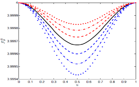
Figure 1: The plot shows the variation of QFI $\mathcal{F}_{\theta}^{R};\theta=\pi/4$ over Rob’s cavity in region III as a function of $u:=\frac{1}{2}\eta_{1}/\ln(b/a)$ with $h=0.01$. The solid curve (black) is for $s=0$ with $k=\pm 1$. The dashed, dash-dotted and dotted curves are, respectively, for $s=\frac{1}{4}$, $\frac{1}{2}$,$\frac{3}{4}$, in k=1 (blue) above the solid curve and k=-1 (red) below the solid curve.

Now let us consider the case for the fermionic mode in Rob’s cavity in region III. In this case, quantum part of the QFI, $F_{\theta}=0$. Thus the only contribution to QFI, $\mathcal{F}_{\theta}^{R}$, is due to its classical part, $F_{c}$. Working pertubatively, as a result, we have

$$\frac{\left(p_{1}^{\prime}\right)^{2}}{p_{1}}= \frac{\sin^{2}2\theta\left(1-f_{k}h^{2}\right)^{2}}{\cos^{2}\theta+\left(-\cos^{2}\theta f_{k}^{-\nu}+\sin^{2}\theta f_{k}^{\nu}\right)h^{2}}$$

$$= 4\sin^{2}\theta\!\left[\!1\!+\!\left(f_{k}^{-\nu}\!-\!f_{k}^{\nu}\tan^{2}\theta-2f_{k}\right)h^{2}\right],$$ (40a)

$$\frac{\left(p_{2}^{\prime}\right)^{2}}{p_{2}}= 4\cos^{2}\theta\!\left[1+\left(f_{k}^{\nu}\!-\!f_{k}^{-\nu}\cot^{2}\theta\!-\!2f_{k}\right)h^{2}\right],$$ (40b)

where $f_{k}^{+}$, $f_{k}^{-}$ given by (28) can be re-written as

$$f_{k}^{+} = \sum_{p\geq 0}^{\infty}\left|E_{1}^{k-p}\right|^{2}|A_{pk}^{(1)}|^{2},$$ (41a)

$$f_{k}^{-} = \sum_{q<0}^{\infty}\left|E_{1}^{k-q}\right|^{2}|A_{qk}^{(1)}|^{2},$$ (41b)

$$f_{k}: = f_{k}^{+}+f_{k}^{-}=\sum_{p=-\infty}^{\infty}|\mathcal{A}_{pk}^{(1)}|^{2},$$ (41c)

with

$$E1:=\exp\left(\frac{i\pi\eta_{1}}{\ln\left(b/a\right)}\right).$$ (42)

The QFI $\mathcal{F}_{\theta}^{R}$ finally reads

$$\displaystyle\mathcal{F}_{\theta}^{R} = 4-4\frac{\left(\sin^{2}\theta f_{k}^{\nu}+\cos^{2}\theta f_{k}^{-\nu}\right)}{\sin^{2}\theta\cos^{2}\theta}h^{2}.$$ (43)

Since by definition (41), the relations $f_{k}^{\nu}$ and $f_{k}^{-\nu}$ are periodic and non-negative, the QFI over Rob’s subsystem is non-negative and is less than or equal to 4 with $0<\theta<\pi/2$ for the perturbative regime $|k|h\ll 1$. Plots for parameter $\theta=\pi/4$ with $k=\pm 1$ are shown in Fig. 1. Consequently, the QFI of the bipartite composite system, $\mathcal{F}_{\theta}$, is sub-additive. Further, it can be noticed that the QFI shows periodic degradation over Rob’s subsystem depending upon the duration of non-inertial motion of Rob’ cavity. However, following the procedure described in PhysRevD.85.025012 , this periodic degradation can be compensated by tuning the intervals of the inertial and non-inertial motion of the Rob’s cavity.

As an extension to the QFI computation of the two mode state, we evaluate the QFI for a single fermionic mode restricted to one cavity and compare its variation with that of Rob’s cavity subsystem. The same setting of inertial and non-inertial segments of motion is considered for the single cavity with the exception that the reference (inertial) cavity is not employed in this case. The parameter $\theta$ is now encoded in the single fermionic cavity mode and the initial state in region I is, therefore, written as

$$\big{|}\psi_{init}\big{>}=\cos\theta\big{|}0\big{>}+\sin\theta\big{|}1_{k}\big{>}^{\nu}.$$ (44)

The density matrix representation is given by

$$\rho_{\nu}^{S}=\cos^{2}\theta\big{|}0\big{>}\big{<}0\big{|}+\sin^{2}\theta\big{|}1_{k}\big{>}^{\nu\nu}\big{<}1\big{|}+\sin\theta\cos\theta\left(\big{|}0\big{>}^{\nu}\big{<}1\big{|}+\big{|}1\big{>}^{\nu}\big{<}0\big{|}\right).$$ (45)

Using the inside out partial tracing approach PhysRevD.85.025012 and by invoking the unitarity of the perturbed Bogoliubov transformation (15), the reduced density matrix in region III is expressed as

$$\rho_{\nu,k}^{S}\equiv\textup{Tr}_{\neg{k}}\rho_{\nu}^{S} = \left(\cos^{2}\theta(1-f_{k}^{-\nu}h^{2})+\sin^{2}\theta f_{k}^{\nu}h^{2}\right)\big{|}\tilde{0}\big{>}\big{<}\tilde{0}\big{|}+\left(\sin^{2}\theta(1-f_{k}^{\nu}h^{2})+\cos^{2}\theta f_{k}^{-\nu}h^{2}\right)\big{|}\tilde{1}_{k}\big{>}^{\nu\nu}\big{<}\tilde{1}_{k}\big{|}$$ (46)

$$+\sin\theta\cos\theta\left(\left(G_{k}+\mathcal{A}_{kk}^{(2)}\right)\big{|}\tilde{0}\big{>}^{\nu}\big{<}\tilde{1}_{k}\big{|}+h.c\right).$$

Since both the eigenvalues $\{p_{i}\}=\{1,0\}$ of the unperturbed part are non-degenerate, therefore the second order correction to these eigenvalues can be obtained using standard perturbation theory as described in bransden2000quantum . The non-zero eigenvalues of the evolved state are given by

$$\{p_{i}\}=\left\{1-\left(\cos^{4}\theta f_{k}^{-\nu}+\sin^{4}\theta f_{k}^{\nu}\right)h^{2},\left(\cos^{4}\theta f_{k}^{-\nu}+\sin^{4}\theta f_{k}^{\nu}\right)h^{2}\right\}.$$ (47)

The corresponding normalized eigenvectors are

$$\big{|}\Phi_{1}\big{>} = \frac{1}{\sqrt{N}}\left\{\begin{array}[]{cc}G_{k}\left(\cos\theta-\alpha\sin\theta\right)&\left(\sin\theta+\alpha\cos\theta\right)\end{array}\right\},$$ (48b)

$$\big{|}\Phi_{2}\big{>} = \frac{1}{\sqrt{N}}\left\{\begin{array}[]{cc}-G_{k}\left(\sin\theta+\bar{\alpha}\cos\theta\right)&\left(\cos\theta-\bar{\alpha}\sin\theta\right)\end{array}\right\},$$ (48d)

where $N=1+|\alpha|^{2}$ is as usual the normalization constant and $\alpha$ is defined as

$$\alpha=\sin\theta\cos\theta\biggl{[}\frac{1}{2}\cos 2\theta f_{k}+\left(f_{k}^{-\nu}-f_{k}^{\nu}\right)+i\textup{Im}\left(G_{k}\bar{\mathcal{A}}_{kk}^{(2)}\right)\biggr{]}h^{2}.$$ (49)

The classical contribution to the QFI is given by

$$F_{c} = \sum_{i}\frac{(p_{i}^{\prime})^{2}}{p_{i}}$$ (50)

$$= 16\cos^{2}\theta\sin^{2}\theta\frac{\left(\cos^{2}\theta f_{k}^{-\nu}-\sin^{2}\theta f_{k}^{\nu}\right)^{2}}{\left(\cos^{4}\theta f_{k}^{-\nu}+\sin^{4}\theta f_{k}^{\nu}\right)}h^{2}+O(h^{4}).$$

The second term involved in the QFI, namely the quantum contribution due to the individual pure states, is computed as follows

$$F_{\theta;i} = 4\sum_{i}p_{i}\left(\big{<}\Phi^{\prime}_{i}|\Phi^{\prime}_{i}\big{>}-\big{|}\big{<}\Phi_{i}|\Phi^{\prime}_{i}\big{>}\big{|}^{2}\right)$$ (51)

$$= 4+4\left\{\cos 4\theta f_{k}+2\cos 2\theta\left(f_{k}^{-\nu}-f_{k}^{\nu}\right)\right\}h^{2}.$$

Further, the quantum contribution due to the mixture of pure states can be expressed as

$$F_{\theta;ij} = 8\sum_{i\neq j}\frac{p_{i}p_{j}}{p_{i}+p_{j}}\big{|}\big{<}\Phi_{i}|\Phi^{\prime}_{j}\big{>}\big{|}^{2}$$ (52)

$$= 16\left(\cos^{4}\theta f_{k}^{-\nu}+\sin^{4}\theta f_{k}^{\nu}\right)h^{2}.$$

Finally, using the relations (50)-(52), the QFI for the single fermionic mode confined to the single cavity can be expressed as

$$\mathcal{F}_{\theta}^{S}=F_{c}+F_{\theta;i}-F_{\theta;ij}.$$ (53)

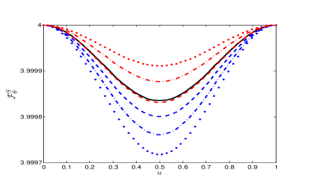
Figure 2: The plots show the variation of QFI $\mathcal{F}_{\theta}^{S}$; $\theta=\pi/4$, of a single fermionic mode within one cavity in region III as a function of $u:=\frac{1}{2}\eta_{1}/\ln(b/a)$ with $h=0.01$. The solid curve (black) is for $s=0$ with $k=\pm 1$. The dashed, dash-dotted and dotted curves are, respectively, for $s=\frac{1}{4}$, $\frac{1}{2}$,$\frac{3}{4}$, in k=1 (blue) and k=-1 (red).

As shown in Fig. 2, the QFI behavior in the case of single Dirac field mode confined to the single cavity is similar to that of the Rob’s cavity subsystem (Fig. 1). However, it is different from the QFI variation (39) of the bipartite or composite system which remains invariant and shows no degradation up to the second order corrections.

V Quantum Fisher Information for the Werner state

We have studied the behavior of Fisher information for the entangled confined modes of cavities of Alice and Bob, where the amount of entanglement is controlled by the parameter $\theta$. We have found the invariance of Fisher information regardless of the parameter $\theta$ up to the order $h^{2}$. Therefore it is natural to ask whether the degrade of entanglement does not affect on the Fisher information. Here, we study the dynamics of QFI for the Werner state, which is a depolaring state of the $\theta$ parameterized two-qubit pure entangled state. For this purpose, we consider the initial two qubit Werner state in region I given by

$$\rho_{\nu}=r\left(\cos\theta\big{|}0\big{>}\big{|}0\big{>}+\sin\theta\big{|}1_{m}\big{>}^{\mu}\big{|}1_{k}\big{>}^{\nu}\right)\left(\cos\theta\big{<}0\big{|}\big{<}0\big{|}+\sin\theta^{\mu}\big{<}1_{m}\big{|}^{\nu}\big{<}\big{|}1_{k}\big{|}\right)+\frac{1-r}{4}\mathbb{I},$$ (54)

where the parameter $r$ indicates the mixedness of the pure entangled two qubit state and the maximally mixed bipartite state. Considering the perturbed evolution of the state in Rob’s cavity from region I to region III in the similar fashion as discussed earlier, we transform the density matrix part confined to Rob’s cavity in terms of Rob’s Region (III) basis to the order $h^{2}$ with the help of (22) and (23). Afterwards, by exploiting the unitarity of the Bogoliubov transformation (15) and applying the partial trace as described in PhysRevD.85.025012 , the reduced density matrix in the region III is expressed as

$$\rho_{{}_{W};\nu,k,} = r\Bigl{[}\cos^{2}\theta\big{|}0\big{>}_{A}\big{<}0\big{|}\otimes\Big{\{}\left(1-f_{k}^{-\nu}h^{2}\right)\big{|}\tilde{0}\big{>}_{III}\big{<}\tilde{0}\big{|}+f_{k}^{-\nu}h^{2}\big{|}\tilde{1}_{k}\big{>}_{III}\big{<}\tilde{1}_{k}\big{|}\Big{\}}+\sin\theta\cos\theta\Big{\{}\left(G_{k}+\mathcal{A}_{kk}^{\left(2\right)}h^{2}\right)$$ (55)

$$\times\big{|}0\big{>}^{\mu}_{A}\big{<}1_{m}\big{|}\otimes\big{|}\tilde{0}\big{>}^{\nu}_{III}\big{<}\tilde{1}_{k}\big{|}\pm h.c\Big{\}}+\sin^{2}\theta\big{|}1_{m}\big{>}^{\mu\mu}_{A}\big{<}1_{m}\big{|}\otimes\Big{\{}\left(1-f_{k}^{\nu}h^{2}\right)\big{|}\tilde{1}_{k}\big{>}^{\nu\nu}_{III}\big{<}\tilde{1}_{k}\big{|}+f_{k}^{\nu}h^{2}\big{|}\tilde{0}\big{>}_{III}\big{<}\tilde{0}\big{|}\Big{\}}\Bigr{]}$$

$$+r^{c}\Bigl{[}\left(\big{|}0\big{>}_{A}\big{<}0\big{|}+\big{|}1_{m}\big{>}^{\mu\mu}_{A}\big{<}1_{m}\big{|}\right)\otimes\Big{\{}\left(1+g_{k}^{\nu}h^{2}\right)\big{|}\tilde{0}\big{>}_{III}\big{<}\tilde{0}\big{|}+\left(1+g_{k}^{-\nu}h^{2}\right)\big{|}\tilde{1}_{k}\big{>}_{III}\big{<}\tilde{1}_{k}\big{|}\Big{\}}\Bigr{]},$$

where $r^{c}$ and $g_{k}^{\pm\nu}$ are defined as

$$r^{c} = \frac{1-r}{4},$$ (56a)

$$g_{k}^{\pm\nu} = f^{\pm\nu}_{k}-f^{\mp\nu}_{k}.$$ (56b)

Thus the perturbed density matrix can be expressed in the compact form as

$$\rho_{{}_{W};\nu,k}=\rho_{{}_{W};\nu,k}^{(0)}+\rho_{{}_{W};\nu,k}^{(2)}h^{2}.$$ (57)

The unperturbed part of the density matrix, $\rho_{{}_{W};\nu,k}^{(0)}$, admits the same set of the eigenvectors as obtained for the two mode pure state in Sec. IV corresponding to the respective unperturbed eigenvalues

$$\textup{EigenVal}\left(\rho_{{}_{W};\nu,k}^{\left(0\right)}\right)=\{r+r^{c},r^{c},r^{c},r^{c}\}.$$ (58)

Two explicit cases arise for $r=0$ and $r=1$. For $r=0$, the unperturbed density matrix represents the maximally mixed state, with standard basis and degenerate eigenvalue of $p_{1,2,3,4}^{(0)}=1$. In this case, the QFI with respect to the parameter $\theta$ yields a trivial result, $\mathcal{F}_{\theta}=0$. For $r=1$, the situation is exactly the same as described in the Sec. IV. Therefore we restrict the value of $r$, in the open interval $0<r<1$.

It can be noted that, the eigenvalues $r+r^{c}$ and $r^{c}$ of the unperturbed part of the density matrix denote the non-degenerate and triply degenerate cases, respectively. Therefore, following the perturbative procedure prescribed in reed1975fourier ; bransden2000quantum and used in the previous section for the non-degenerate and degenerate cases, the eigenvalues of the reduced density matrix $\rho_{{}_{W};\nu,k}$ in the region III are

$$\{p_{i}\}=\Bigl{\{} r+r^{c}-r\left(\cos^{2}\theta f_{k}^{-\nu}+\sin^{2}\theta f_{k}^{\nu}\right)h^{2}+r^{c}\left(\cos^{2}\theta g_{k}^{\nu}+\sin^{2}\theta g_{k}^{-\nu}\right)h^{2},r^{c}+r^{c}\left(\sin^{2}\theta g_{k}^{\nu}+\cos^{2}\theta g_{k}^{-\nu}\right)h^{2},$$

$$r^{c}+r^{c}g_{k}^{-\nu}h^{2}+rf_{k}^{-\nu}\cos^{2}\theta h^{2},r^{c}+r^{c}g_{k}^{\nu}h^{2}+rf_{k}^{\nu}\sin^{2}\theta h^{2}\Bigr{\}}.$$ (59)

From (59), it can be seen that the perturbed density matrix satisfies the density matrix conditions, $p_{i}\geq 0;\forall i$ and $\sum_{i}p_{i}=1$. Furthermore, the classical contribution, to the QFI, $F_{c}$, vanishes for $0<r<1$. This is due to the fact that for each eigenvalue, $p_{i}$, the expression $(\partial_{\theta}p_{i})^{2}/p_{i}$ has the leading term of order $h^{4}$. Hence, $F_{c}=0+O(h^{4})$. However, it is important to note that for the special case of $r=1$, the classical contribution $F_{c}$ is non-vanishing and is given by (38). Next, the corresponding perturbed eigenvectors are

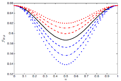
Figure 3: The plot shows the variation of QFI $\mathcal{F}_{{}_{W};\theta}$ at $\theta=\pi/4$ for bipartite Werner state in region III as a function of $u:=\frac{1}{2}\eta_{1}/\ln(b/a)$ with fixed value: $h=0.01$, $r=1/3$. The solid curve (black) is for $s=0$ with $k=\pm 1$. The dashed, dash-dotted and dotted curves are, respectively, for $s=\frac{1}{4}$, $\frac{1}{2}$,$\frac{3}{4}$, in k=1 (blue) above the solid curve and k=-1 (red) below the solid curve.

$$|\Phi_{1}\big{>}= \frac{1}{\sqrt{N}}\left\{\begin{array}[]{cccc}G_{k}\left(\cos\theta-\frac{\beta}{r}\sin\theta\right)&0&0&\sin\theta\!+\!\frac{\beta}{r}\cos\theta\\ \end{array}\right\},$$ (60b)

$$|\Phi_{2}\big{>}= \frac{1}{\sqrt{N}}\!\!\left\{\begin{array}[]{cccc}\!\!-G_{k}\left(\sin\theta+\frac{\bar{\beta}}{r}\cos\theta\right)&0&0&\cos\theta\!-\!\frac{\bar{\beta}}{r}\sin\theta\\ \end{array}\!\!\right\},$$ (60d)

$$|\Phi_{3}\big{>}= \left\{\begin{array}[]{cccc}0&1&0&0\\ \end{array}\right\},$$ (60f)

$$|\Phi_{4}\big{>}= \left\{\begin{array}[]{cccc}0&0&1&0\\ \end{array}\right\},$$ (60h)

where $N=1+|\beta|^{2}/r^{2}$ is the normalization constant and $\beta$ is defined as

$$\beta=\sin\theta\cos\theta\Bigl{[}\frac{f_{k}^{-\nu}-f_{k}^{\nu}}{2}+ir\textup{Im}(G_{k}\bar{\mathcal{A}}_{kk}^{(2)})\Bigr{]}h^{2}.$$ (61)

The quantum contribution due to the individual quantum states is

$$F_{\theta;i}=4\sum_{i}p_{i}\mathcal{F}_{\theta,i}=4\biggl{[}\frac{1+r}{2}+\Bigl{\{}\frac{1+r}{2r}\cos 2\theta\bigl{(}f_{k}^{-\nu}-f_{k}^{\nu}\bigr{)}-r\bigl{(}\cos^{2}\theta f_{k}^{-\nu}+\sin^{2}\theta f_{k}^{\nu}\bigr{)}\Bigr{\}}h^{2}\biggr{]}.$$ (62)

Next, we have the contribution to the QFI due to the mixture, which is given by

$$F_{\theta;ij}= 8\sum_{i\neq j}\mathcal{F}_{\theta;ij}$$

$$= 16\biggl{[}\frac{1+2r-3r^{2}}{8\left(1+r\right)}\Bigl{\{}1+\frac{\cos 2\theta}{r}\left(f_{k}^{-\nu}-f_{k}^{\nu}\right)h^{2}\Bigr{\}}+\left(1-r\right)r\Bigl{\{}\frac{1+3r}{4\left(1+r\right)^{2}}\left(\sin^{2}\theta f_{k}^{\nu}+\cos^{2}\theta f_{k}^{-\nu}\right)$$

$$-\frac{1}{2\left(1+r\right)}\left(\sin^{2}\theta f_{k}^{-\nu}+\cos^{2}\theta f_{k}^{\nu}\right)\Bigr{\}}h^{2}\biggr{]}.$$ (63)

The QFI $\mathcal{F}_{\theta}$ of the Werner state, (55), with $0<r<1$ can therefore be expressed using (62) and (63) as

$$\mathcal{F}_{\theta}=F_{\theta}=F_{\theta;i}-F_{\theta;ij}.$$ (64)

It can be noticed that for $r<1$, the classical contribution, $F_{c}$, is zero while the quantum mixture, $F_{\theta;ij}$, is non-zero. However, for $r=1$, the classical contribution is non-vanishing while the mixture term disappears and we obtain the same result (39) as a special case. Unlike the pure two qubit state case earlier discussed in Sec. IV, it can be seen from (64) that the QFI of the Werner state is affected due to the inertial and non-inertial segments of Rob’s cavity motion for mixing parameter $r\in\left(0,1\right)$. Furthermore, the QFI of the Werner state exhibits periodic degradation for $r\in\left(0,1\right)$ as shown in Fig. 3 for the case of $\theta=\pi/4$ and $r=1/3$. This periodic degradation, however, can be avoided by fine-tuning the duration of inertial and non-inertial trajectories for Rob’s cavity.
The effect of mixing parameter $r$ is also investigated and is shown in Fig. 4.

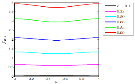
Figure 4: The plot shows the variation of QFI $\mathcal{F}_{{}_{W};\theta}$ at $\theta=\pi/4$ for bipartite Werner state in region III as a function of $u:=\frac{1}{2}\eta_{1}/\ln(b/a)$ with $h=0.01$. The colored curves from bottom to top correspond to the values of parameter $r=0.1,0.33,0.5,0.66,0.85,0.99$, respectively. The mode in Rob’s cavity is kept fixed at $k=1$ with $s=0$ for all these curves.

It is shown that as the parameter $r$ varies(in the region of $0<r<1$), the QFI of Werner state is affected by the inertial and non-inertial segments of motion of Rob’s cavity.

The QFI distribution over subsystems of Alice’s and Rob’s cavity modes can be evaluated using a procedure similar to that of Sec. IV.3. The QFI $\mathcal{F}_{\theta}^{A}$ over Alice’s cavity in region III is given by

$$\mathcal{F}_{\theta}^{A}=\frac{4r^{2}\sin^{2}2\theta}{1-r^{2}\cos^{2}2\theta}.$$ (65)

The QFI $\mathcal{F}_{\theta}^{R}$ over Rob’s cavity in region III is given by

$$\mathcal{F}_{\theta}^{R}= \frac{4r^{2}\sin^{2}2\theta}{1-r^{2}\cos^{2}2\theta}\biggl{[}1-2f_{k}h^{2}-\frac{r\cos 2\theta}{1-r\cos^{2}2\theta}\Bigl{\{}4r\bigl{(}\cos^{2}\theta f_{k}^{-\nu}\!\!\!-\!\sin^{2}\theta f_{k}^{\nu}\bigr{)}\!+\!2(1\!-\!r)\bigl{(}f_{k}^{-\nu}\!\!-\!\!f_{k}^{\nu}\bigr{)}\Bigr{\}}h^{2}\!\biggr{]}.$$ (66)

Since the QFI for each cavity mode is non-negative and has a maximum value of 4, therefore the QFI distribution over subsystems is sub-additive.

VI Conclusion and Discussion

We investigated the effect of relativistic motion on the quantum Fisher information of the $\left(1+1\right)$ Dirac field modes confined to cavities. For this purpose, we considered a realistic scheme for two cavities. In our scenario, the modes of a massless Dirac field were confined to the two cavities with Dirichlet s boundary conditions, where one of the cavities remained inertial, while the other underwent the segments of inertial and non-inertial motion with uniform acceleration. The acceleration was assumed to be very small and its effects were analyzed in a perturbative regime. We considered a $\theta$ parameterized two-qubit pure entangled state and a Werner state. In contrast to the degradation of entanglement due to the relativistic motion between the cavities, the quantum Fisher information of the pure composite system $\mathcal{F}_{\theta}$ with respect to parameter $\theta$ was found to be invariant under the same conditions. However, in the case of the Werner state, which is a depolaring state of the $\theta$ parameterized two-qubit pure entangled state, the quantum Fisher information displayed periodic degradation, due to the inertial and non-inertial segments of motion. Furthermore, the quantum Fisher information over Rob’s cavity showed periodic degradation behavior depending upon the parameter $\theta$ as well as the uniform acceleration for both the two qubit pure state and Werner state. The quantum Fisher information over Alice’s cavity remained invariant throughout the motion of Rob’s cavity for the two qubit pure state, whereas for the Werner state it was affected by the mixing parameter of the Werner state. The subadditivity of the quantum Fisher information was held regardless of the pure composite system or the Werner state.

References

- (1) S. L. Braunstein, C. M. Caves, and G. J. Milburn, Annals of Physics 247, 135 (1996).
- (2) S. L. Braunstein, and C. M. Caves, Phys. Rev. Lett. 72, 3439 (1994).
- (3) C. W. Helstorm, Quantum detection and estimation theory, Mathematics in Science and Engineering (Elsevier Science, 1976), ISBN 9780080956329.
- (4) S. Luo, Phys. Rev. Lett. 91, 180403 (2003).
- (5) Y. Watanabe, T. Sagawa, and M. Ueda, Phys. Rev. A 84, 042121 (2011).
- (6) R. A. Fisher, in Mathematical Proceedings of the Cambridge Philosophical Society (Cambridge Univ. Press, 1925), vol. 22, pp. 700-725.
- (7) A. S. Holevo, Probabilistic and statistical aspects of quantum theory, Mathematics in Science and Engineering (Springer, 2011), ISBN 9788876423758.
- (8) S. W. Hawking, Phys. Rev. D 14, 2460 (1976).
- (9) W. G. Unruh, Phys. Rev. D 14, 870 (1976).
- (10) R. M. Wald, Quantum Field Theory in Curved Spacetime and Black Hole Thermodynamics, (University of Chicago Press, Chicago, 1994).
- (11) A. Fabbri, and J.Navarro-Salas, Modeling black hole evaporation, (World Scientific, 2005).
- (12) A. Peres, and D. R. Terno, Rev. Mod. Phys. 76, 93 (2004).
- (13) P. M. Alsing, and I. Fuentes, Classical and Quantum Gravity 84, 224001 (2012).
- (14) D. E. Bruschi, J. Louko, E. Martín-Martínez, A. Dragan, and I. Fuentes, Phys. Rev. A 82, 042332 (2010); J. Chang and Y.Kwon,Phys. Rev. A 85, 032302 (2012); J. Chang and Y.Kwon, Int.J.Theo.Phys. 54, 996 (2015)
- (15) L. C. B. Crispino, A. Higuchi, and G. E. A. Matsas, Rev. Mod. Phys. 80, 787 (2008).
- (16) I. Fuentes-Schuller, and R. B. Mann, Phys. Rev. Lett. 95, 120404 (2005); M. Montero and E. Martin-Martinez, Phys. Rev. A 83, 062323 (2011); M. Montero and E. Martin-Martinez, JHEP 07, 006 (2011); J.Chang and Y.Kwon, Phys. Rev. A 86, 014302 (2012)
- (17) D. E. Bruschi, I. Fuentes, and J. Louko, Phys. Rev. D 85, 061701 (2012).
- (18) N. Friis, A. R. Lee, and D. E. Bruschi, Phys. Rev. A 87, 022338 (2013).
- (19) N. Friis, A. R. Lee, D. E. Bruschi, and J. Louko, Phys. Rev. D 85, 025012 (2012).
- (20) P. M. Alsing, I. Fuentes-Schuller, R. B. Mann, and T. E. Tessier, Phys. Rev. A 74, 032326 (2006).
- (21) A. Datta, Phys. Rev. A 80, 052304 (2009).
- (22) J. Wang, J. Deng, and J. Jing, Phys. Rev. A 81, 052120 (2010).
- (23) E. G. Brown, K. Cormier, E. Martín-Martínez, and R. B. Mann, Phys. Rev. A 86, 032108 (2012); J. Wang, J. Jing, and H. Fan, Phys. Rev. D 90 025032 (2014)
- (24) P. M. Alsing, and G. J. Milburn, Phys. Rev. Lett. 91, 180404 (2003).
- (25) M. Aspachs, G. Adesso, and I. Fuentes, Phys. Rev. Lett. 105, 151301 (2010).
- (26) Y. Yao, X. Xiao, L. Ge, X.-g. Wang, and C.-p. Sun, Phys. Rev. A 89, 042336 (2014); N. Metwally, arXiv:1609.02092
- (27) M. Ahmadi, D. E. Bruschi, C. Sabín, G. Adesso, and I. Fuentes, Sci. Rep. 4, 4996 (2014).
- (28) D. Bures, Trans. Amer. Math. Soc. 135, 199 (1969).
- (29) M. G. A. Paris, Int. J. of Quantum Inform. 07,125 (2009).
- (30) Y. M. Zhang, X. W. Li, W. Yang, and G. R. Jin, Phys. Rev. A 88, 043832 (2013).
- (31) A. R. Lee, Ph.D. thesis, University of Nottingham, 2013 (arXiv:1309.4419).
- (32) M. Reed, and B. Simon, Methods of Modern Mathematical Physics, (Academic Press, New York, 1975).
- (33) B. H. Bransden, and C. J. Joachain, Quantum mechanics, (Prentice hall Harlow, 2000).
- (34) W. Zhong, Z. Sun, J. Ma, X. Wang, and F. Nori, Phys. Rev. A 87, 022337 (2013).
- (35) X.- M. Lu, S. Luo, and C. H. Oh, Phys. Rev. A 86, 022342 (2012).
- (36) N. Friis, A. R. Lee, K. Truong, C. Sabín, E. Solano, G. Johansson, and I. Fuentes, Phys. Rev. Lett. 110, 113602 (2013).
- (37) M. Ahmadi, D. E. Bruschi, and I. Fuentes, Phys. Rev. D 89, 065028 (2014).
- (38) Werner, R. F., Phys. Rev. A 40, 4277 (1989).