Separation of equilibrium part from an off-equilibrium state produced by relativistic heavy ion collisions using a scalar dissipative strength

Abstract

We have proposed a novel way to specify the initial conditions of a dissipative fluid dynamical model for a given energy density $\varepsilon=u_{\mu}T^{\mu\nu}u_{\nu}$ and baryon number density $n=N^{\mu}u_{\mu}$, which does not impose the so-called Landau matching condition for an off-equilibrium state. In addition to usual two parameters for equilibrium part, i.e., $\alpha\equiv\mu/T$, $\beta\equiv 1/T$ (where $T$ is separation temperature and $\mu$ is separation chemical potential introduced to separate equilibrium part from the off-equilibrium state), a dissipative strength $\gamma$ is newly introduced to specify the off-equilibrium state. These $\alpha$, $\beta$ and $\gamma$ can be uniquely determined by $\varepsilon$, $n$ and $P_{\rm eq}(\alpha,\beta)+\Pi=-1/3\Delta_{\mu\nu}T^{\mu\nu}$ consisting of both kinetic theoretical definitions and the thermodynamical stability condition. For $\gamma<10^{-3}$, $T$ and $\mu$ are almost independent of $\gamma$, which means that the Landau matching condition is approximately satisfied. However, this is not the case for $\gamma\gtrsim 10^{-3}$.

1 Introduction

Relativistic hydrodynamical models have been applied to studies of matter that is produced in high-energy hadron or nuclear collisions. Fluid dynamical descriptions, in particular, provide a simple picture of the space-time evolution of the hot/dense matter produced by ultra-relativistic heavy-ion collisions at RHIC and LHC Heinz2013_1 ; Heinz2013_2 . It is expected that this simple picture makes it possible to investigate the strongly interacting quark and gluon matter present at the initial stage of the collisions. The fluid model assumes that there exist local quantities of the matter such as energy density, pressure and so on. In particular, it is considered that the pressure gradients of the matter causes collective phenomena Gustafsson1984 ; Hirano:2008hy . These expected phenomena have been successfully observed as an elliptic flow coefficient $v_{2}$ in the CERN SPS experiment NA49 NA491998 , at RHIC experiment PhysRevC.77.054901 ; PhysRevLett.98.162301 ; PhysRevLett.98.242302 and recent ALICE experiments in LHC Snellings2014 including the higher order flow harmonic $v_{n}$ for ($n=3,4$). These have been observed as a function of various characteristics, including the transverse momentum $p_{\rm T}$ or rapidity $y$ and so on. Hence, the hydrodynamical model has been widely accepted because of such experimental evidences. To investigate the properties of the quark and gluon matter created during such ultra-relativistic heavy-ion collisions more precisely, it is necessary to consider the effects of the viscosities and corresponding dissipation MurongaPRC69 . These effects are introduced into the hydrodynamic simulations and a detailed comparison between simulation and experimental data is made (see, for example, Ref.SongPRC89 ). However, as several authors have noted, dissipative hydrodynamics is not yet completely understood and there are issues associated to the determination of the hydrodynamical flow TsumuraPLB646 ; TsumuraPLB690 ; Van2013 (see also, Ref. Arnold2014 ). In this article, the Landau matching (fitting) condition that is necessary to specify the initial conditions for dissipative fluid dynamics is discussed. This may be related to the issue of defining the local rest frame TsumuraPLB690 .

The fundamental equations of relativistic fluid dynamics are defined by the conservation laws of energy-momentum and the charge (in this paper, we assume the net baryon density as the conserved charge),

$$\partial_{\mu}T^{\mu\nu}(x)=0,$$ (1a)

$$\partial_{\mu}N^{\nu}(x)=0.$$ (1b)

Here, $T^{\mu\nu}$ and $N^{\mu}$ are respectively the energy-momentum tensor and the conserved charge current at a given point in space-time $x$, which can be obtained by a coarse-graining procedure KodamaEPJA48 with some finite size (fluid cell size), $l_{\rm fluid}$. Hence, the fluid dynamical model expressed as a coarse-graining theory describing macroscopic phenomena can be derived from the underlying kinetic theory. In the case of a perfect fluid limit, the microscopic collision time scale $\tau_{\rm micro}$ is much shorter than the macroscopic evolution time scale $\tau_{\rm macro}$PhysRevC.73.034904 , thus

$$\tau_{\rm macro}\gg\tau_{\rm micro}.$$ (2)

If the condition in eq.(2) is satisfied, the distribution function instantaneously relaxes to its local equilibrium form. In the local rest frame of the fluid, i.e., the frame in which the fluid velocity is given by $u^{\mu}(x)=(1,0,0,0)$, the local equilibrium distribution functions for particles and for anti-particles are respectively given (within the Boltzmann approximation) as

$$f_{{\bf k}0}(x)=\exp[\frac{-k_{\mu}u^{\mu}(x)+\mu_{0}(x)}{T_{0}(x)}],$$ (3a)

$$\bar{f}_{{\bf k}0}(x)=\exp[\frac{-k_{\mu}u^{\mu}(x)-\mu_{0}(x)}{T_{0}(x)}],$$ (3b)

where $k^{\mu}$ is a four momentum vector of a particle or an anti-particle within a cube the coarse-graining scale $l_{\rm fluid}$ on a side (fluid cell). We decompose $k^{\mu}$ by using the local flow vector $u^{\mu}$, i.e., $k^{\mu}=(k^{\lambda}u_{\lambda})u^{\mu}+k^{\langle\mu\rangle}$ where $k^{\mu}u_{\mu}\equiv E_{\bf k}$ is a scalar and $k^{\langle\mu\rangle}\equiv\Delta_{\nu}^{\mu}k^{\nu}$ is a vector, which is orthogonal to $u^{\mu}$. In the local rest frame, the scalar $E_{\bf k}$ coincides with the zero-th component of the four vector, energy of the classical particle, $k^{0}$. The projection tensor onto the 3-space that is orthogonal to the flow velocity is defined by $\Delta^{\mu\nu}\equiv g^{\mu\nu}-u^{\mu}u^{\nu}$ with $g^{\mu\nu}$ being the metric tensor, $g^{\mu\nu}={\rm diag}(+1,-1,-1,-1)$. $T_{0}(x)$ and $\mu_{0}(x)$ are the equilibrium temperature and chemical potential respectively. When the distribution function is given by eq.(3), the energy-momentum tensor and the net baryon number current vector are defined as

$$T^{\mu\nu}_{\rm eq} = \int\!\!\frac{d^{3}{\bf k}k^{\mu}k^{\nu}}{(2\pi)^{3}k^{0}}\Big{[}f_{{\bf k}0}(x)+\bar{f}_{{\bf k}0}(x)\Big{]}$$ (4a)

$$= \varepsilon_{\rm eq}u^{\mu}u^{\nu}-P_{\rm eq}(\varepsilon_{\rm eq},n_{\rm eq})\Delta^{\mu\nu},$$

$$N^{\mu}_{\rm eq} = \int\!\!\frac{d^{3}{\bf k}~{}k^{\mu}}{(2\pi)^{3}k^{0}}\Big{[}f_{{\bf k}0}(x)-\bar{f}_{{\bf k}0}(x)\Big{]}$$ (4b)

$$= n_{\rm eq}u^{\mu},$$

respectively, where $\varepsilon_{\rm eq}$ is the energy density in the local rest frame, $n_{\rm eq}$ is the net baryon density in the local rest frame, and $P_{\rm eq}$ is the pressure in the equilibrium state.

If the fluid expands very rapidly (i.e., the macroscopic evolution time scale $\tau_{\rm macro}$ becomes shorter), especially for fluids produced by ultra-relativistic heavy-ion collisions, equation (2) may not be satisfied everywhere in the fluid during the early stages. In such cases, microscopic processes cannot keep pace with the changes in local energy and baryon density; therefore, we can write the following equation:

$$\tau_{\rm micro}\gtrsim\tau_{\rm macro}.$$ (5)

Under the condition eq.(5), the distribution function in the local rest frame does not obey the local equilibrium form eq.(3) and hence we have

$$f_{\bf k}(x)=f_{{\bf k}0}[T(x),\mu(x)]+\delta f_{\bf k}(x),$$ (6a)

$$\bar{f}_{\bf k}(x)=\bar{f}_{{\bf k}0}[T(x),\mu(x)]+\delta\bar{f}_{\bf k}(x),$$ (6b)

where $\delta f_{\bf k}$ and $\delta\bar{f}_{\bf k}$ are the deviations from the corresponding equilibrium distribution functions. We define a temperature $T(x)$ and chemical potential $\mu(x)$ (hereafter the separation temperature and separation chemical potential, respectively) that is distinguished from the equilibrium temperature $T_{0}(x)$ and chemical potential $\mu_{0}(x)$ because we assume that $\delta f_{\bf k}$ and $\delta\bar{f}_{\bf k}$ also contribute to the energy and baryon number density of the system. In the inside of the fluid cell, within scales less than the coarse-graining scale $l_{\rm fluid}$, the extremely rapid expansion of matter causes additional tiny disturbances to the local flow velocity field $u^{\mu}(x)$. Although such tiny disturbance in the flow vectors may be cancelled out by defining a new local rest frame (because of the randomness of such tiny disturbances), it also causes a disturbance in the distribution function $\delta f_{\bf k}(x)$ and $\delta\bar{f}_{\bf k}(x)$. For simplicity, we assume that the fluid considered is stable against such disturbances; otherwise, the disturbance would escalate and the flow would eventually become turbulent. The space-time evolution of the disturbance flow is independent from that of main background flow even if heat is supplied by the main background flow. Since the disturbance flow has no mechanism for obtaining energy other than heat originated from the shear viscosity of the main background flow, it is finally dissipated as heat. Thus, the disturbances, $\delta f_{\bf k}$ and $\delta\bar{f}_{\bf k}$, do not belong to any equilibrium state. As the macroscopic evolution time scale $\tau_{\rm macro}$ grows longer due to the expansion of matter and the pressure gradients of the fluid decrease, $\delta f_{\bf k}$ and $\delta\bar{f}_{\bf k}$ approaches to zero (an assumption of hydrodynamic stability), and the condition eq.(2) is restored and local equilibrium is achieved.

The question we now consider is how to find local separation temperature $T(x)$ and chemical potential $\mu(x)$ in eq.(6) from a given off-equilibrium state characterized by

$$T^{\mu\nu}(x) \equiv \int\!\!\frac{d^{3}{\bf k}k^{\mu}k^{\nu}}{(2\pi)^{3}k^{0}}\Big{[}f_{\bf k}(x)+\bar{f}_{\bf k}(x)\Big{]},$$ (7a)

$$N^{\mu}(x) \equiv \int\!\!\frac{d^{3}{\bf k}~{}k^{\mu}}{(2\pi)^{3}k^{0}}\Big{[}f_{\bf k}(x)-\bar{f}_{\bf k}(x)\Big{]}.$$ (7b)

Usually the local separation temperature $T(x)$ and chemical potential $\mu(x)$ in eq.(6) are determined by imposing the so-called Landau matching conditions Landau1959 ; Israel118 ; PhysRevC.73.034904 ; Heinz:2009xj

$$\delta T^{\mu\nu}u_{\mu}u_{\nu}=0,$$ (8a)

$$\delta N^{\mu}u_{\mu}=0,$$ (8b)

where $\delta T^{\mu\nu}\equiv T^{\mu\nu}-T_{\rm eq}^{\mu\nu}$ and $\delta N^{\mu}\equiv N^{\nu}-N_{\rm eq}^{\mu}$ are the deviation of the energy-momentum tensor and the baryon charge current from the matching state, respectively. In this procedure, it is necessary to select a Lorentz frame. There are usually two natural choices for the Lorentz frame, namely the Landau frame Landau1959 and the Eckart frame Eckart1940 . If the Landau frame is employed, for example, the local flow velocity $u^{\mu}$ is determined by the eigenvector of the following eigenvalue equation,

$$u_{\mu}T^{\mu\nu}=\varepsilon u^{\nu},$$ (9a)

where the eigenvalue $$\varepsilon T \mu \varepsilon=\varepsilon_{\rm eq}(T,\mu)$$ is the energy density measured in the rest frame. In the Landau matching condition, shown in eq.(8a), the energy density should be matched to an energy density in an equilibrium state parameterized by a temperature and a chemical potential , i.e., . Using the flow velocity obtained in eq.(9a), we obtain the following equation:

$$N^{\mu}=nu^{\mu}+V^{\lambda}\Delta_{\lambda}^{\mu}$$ (9b)

for the net baryon number current. Then eq.(8b) yields $n=n_{\rm eq}(T,\mu)$. In this way it is possible to determine $T$ and $\mu$ from $\varepsilon=\varepsilon_{\rm eq}(T,\mu)$ and $n=n_{\rm eq}(T,\mu)$. However, if the Eckart frame is employed, a different temperature $T^{\prime}$ and chemical potential $\mu^{\prime}$ may be obtained as compared to those derived in the Landau frame. For a paper which deals with the issue of the frame in the relativistic dissipative hydrodynamical model, see, for example, Ref.Van2013 . Therefore, for an off-equilibrium states, the temperature and chemical potential which characterize the distribution function for the equilibrium part may be dependent on the frame employed.

Note that, the temperature $T$ and chemical potential $\mu$ are not only dependent on the frame employed but also on the matching condition eq.(8). However, it is not always appropriate, as discussed below. In order to investigate how the matching condition affects the separation to an equilibrium part from an off-equilibrium, one must fix the Lorentz frame to define the fluid velocity. We hereafter use the Landau frame and define a flow vector $u^{\mu}$ as an eigenvector of eq.(9a), but we do not use the Landau-matching condition eq.(8); i.e., the obtained eigenvalue $\varepsilon$ of eq.(9a) is not assumed to be same as an equilibrium energy density $\varepsilon_{\rm eq}$.

In the kinetic approach, since the energy-momentum tensor and the conserved charge current are defined by the second and first moment of the single particle distribution function, the Landau matching conditions eq.(8) are equivalent to the following expressions BiroMolnarEPJA48

$$\int\!\!\frac{d^{3}{\bf k}~{}E_{k}^{2}}{(2\pi)^{3}k^{0}}\Big{[}\delta f_{\bf k}(x)+\delta\bar{f}_{\bf k}(x)\Big{]}=0,$$ (10a)

$$\int\!\!\frac{d^{3}{\bf k}~{}E_{k}}{(2\pi)^{3}k^{0}}\Big{[}\delta f_{\bf k}(x)-\delta\bar{f}_{\bf k}(x)\Big{]}=0.$$ (10b)

Clearly, these conditions strongly constrain the disturbances $\delta f_{\bf k}$ and $\delta\bar{f}_{\bf k}$ and they may distort the distribution function unnaturally. To restore the physical meaning of $\delta f_{\bf k}$ and $\delta\bar{f}_{\bf k}$, it is necessary to exclude the restrictions imposed by eq.(8) and to generalize the Landau matching condition the following form.

$$\delta T^{\mu\nu}u_{\mu}u_{\nu}=\Lambda,\quad\delta n^{\mu}u_{\mu}=\delta n.$$ (11)

Here, $\Lambda$ and $\delta n$ can be considered as the energy density and net baryon number density of the disturbance (tiny turbulent) flow caused by rapid expansion. Except for particles constituting the disturbance flow, it is assumed that the remaining particles in the fluid cell approximately obey the local thermal distribution form $f_{{\bf k}0}$ or $\bar{f}_{{\bf k}0}$. Since the disturbance flow carry finite energy and baryon number, the corresponding separation temperature $T$ and separation chemical potential $\mu$ of the equilibrium part should be different from those obtained at the equilibrium limit, i.e., $T(x)\neq T_{0}(x)$ and $\mu(x)\neq\mu_{0}(x)$. Therefore, to find the separate temperature $T$ and chemical potential $\mu$ in eq.(6), it is required to find find $T$ and $\mu$ as functions of $\delta f_{\bf k}$ and $\delta\bar{f}_{\bf k}$,

$$T = T(\delta f_{\bf k},\delta\bar{f}_{\bf k};T_{0},\mu_{0}),$$ (12a)

$$\mu = \mu(\delta f_{\bf k},\delta\bar{f}_{\bf k};T_{0},\mu_{0}),$$ (12b)

with boundary conditions $T\to T_{0}$ and $\mu\to\mu_{0}$ when the disturbance flow disappears, $\delta f_{\bf k},\delta\bar{f}_{\bf k}\to 0$. The boundary condition corresponds to the so-called Landau matching condition.

In any off-equilibrium state, most literature using the Landau matching condition published to date assumes that $T\equiv T_{0}$ and $\mu\equiv\mu_{0}$. However, in this paper, we consider the problem where $T$ and $\mu$ are dependent on the strength of the off-equilibrium state, i.e., $T$ and $\mu$ are functions of $\delta f_{\bf k}$ and $\delta\bar{f}_{\bf k}$, as seen in eq.(12).

This article is organized as follows. In Section 2, we obtain an expression for eq.(6) using the irreducible tensor expansion technique for the off-equilibrium distribution function, as recently employed by G.S. Denicol and his collaboratorsPhysRevD.85.114047 . We extend the formulation by introducing the general matching condition of eq.(11) and also apply the irreducible tensor expansion technique to an off-equilibrium entropy current and find a condition of thermodynamical stability. Then, we obtain a relation between the quantities introduced by eq.(11) and determine them as functions of $\alpha,\beta$ and $\gamma\equiv\Pi/P_{\rm eq}$. In Section 3, we demonstrate the separation of the corresponding equilibrium state from the given off-equilibrium state, i.e., we determine $T$ and $\mu$ for a given off-equilibrium state characterized by $T_{0}$, $\mu_{0}$, and $\gamma$. We also show an off-equilibrium distribution function and discuss the effects of the strength of the off-equilibrium state $\gamma$. Finally, Section 4 contains conclusions and summary. The derivations of key equations in the relativistic kinetic theory and equations related to irreducible expansion theory are presented in Appendixes A-G.

2 Separation equilibrium part from the off-equilibrium distribution function

2.1 Expansion of the single particle distribution function by irreducible tensors

Consider a relativistically expanding fluid in which microscopic processes cannot keep pace with the quick macroscopic changes. Let us rewrite eq.(6), which is expected the distribution function under the condition eq.(5), as the following form:

$$f_{\bf k}(x)=f_{{\bf k}0}(T[\phi_{\bf k},\bar{\phi}_{\bf k}],\mu[\phi_{\bf k},\bar{\phi}_{\bf k}])\left(1+\phi_{\bf k}\right),$$ (13a)

$$\bar{f}_{\bf k}(x)=\bar{f}_{{\bf k}0}(T[\phi_{\bf k},\bar{\phi}_{\bf k}],\mu[\phi_{\bf k},\bar{\phi}_{\bf k}])\left(1+\bar{\phi}_{\bf k}\right),$$ (13b)

where $\phi_{\bf k}(x)\equiv\delta f_{\bf k}(x)/f_{{\bf k}0}(x)$ and $\bar{\phi}_{\bf k}(x)\equiv\delta\bar{f}_{\bf k}(x)/\bar{f}_{{\bf k}0}(x)$ are deviations from the local thermal equilibrium function eq.(3). The deviations $\phi_{\bf k}(x)$ and $\bar{\phi}_{\bf k}(x)$ involve information about a given off-equilibrium state characterized not only by scalars such as $\Lambda$, $\delta n$, and $\gamma\equiv\Pi/P_{\rm eq}$ but also by vectors and tensors, for example, the heat flow vector $W^{\mu}$, shear tensor $\pi^{\mu\nu}$ of the dissipative fluid and so on. In order to expand $\phi_{\bf k}$ and $\bar{\phi}_{\bf k}$ by those fluid dynamical quantities, it is necessary to use the orthogonal base of irreducible tensors DeGroot:1980dk ; PhysRevD.85.114047 , $\{1,k_{\langle\mu\rangle},\cdots,k_{\langle\mu_{1}}\cdots k_{\mu_{l}\rangle}\}$, where the irreducible tensor of the $l$-rank is defined by

$$k_{\langle\mu_{1}}\cdots k_{\mu_{l}\rangle}\equiv\Delta_{\mu_{1}\cdots\mu_{n}}^{\nu_{1}\cdots\nu_{n}}k_{\nu_{1}}\cdots k_{\nu_{n}},$$ (14)

and the projection tensor $\Delta_{\mu_{1}\cdots\mu_{n}}^{\nu_{1}\cdots\nu_{n}}$ used in eq.(14) are defined in Appendix A (see also Appendix B, C and references DeGroot:1980dk ; PhysRevD.85.114047 ). These irreducible tensors $k_{\langle\mu_{1}}\cdots k_{\mu_{l}\rangle}$ satisfy the following orthogonal condition (for derivation, see Appendix B, C and D),

$$\int\!\!\frac{d^{3}{\bf k}~{}F(E_{\bf k})}{(2\pi)^{3}k^{0}}~{}k^{\langle\mu_{1}}\cdots k^{\mu_{m}\rangle}k_{\langle\nu_{1}}\cdots k_{\nu_{n}\rangle}=\Delta^{\mu 1\cdots\mu_{m}}_{\nu_{1}\cdots\nu_{n}}\delta_{mn}~{}{\cal J}_{m},$$ (15a)

where

$${\cal J}_{m}=\frac{m!}{(2m+1)!!}\int\!\!\frac{d^{3}{\bf k}~{}F(E_{\bf k})}{(2\pi)^{3}k^{0}}[\Delta_{\alpha\beta}k^{\alpha}k^{\beta}]^{m},$$ (15b)

and $F(E_{\bf k})$ is an arbitrary function of the energy $E_{\bf k}$. Since the tensors defined in eq.(14) are orthogonal, we may expand the deviation $\phi_{\bf k}$ and $\bar{\phi}_{\bf k}$ as follows:

$$\phi_{\bf k}(x)\equiv\sum_{l=0}^{\infty}\lambda_{\bf k}^{\langle\mu_{1}\cdots\mu_{l}\rangle}k_{\langle\mu_{1}}\cdots k_{\mu_{l}\rangle},$$ (16a)

$$\bar{\phi}_{\bf k}(x)\equiv\sum_{l=0}^{\infty}\bar{\lambda}_{\bf k}^{\langle\mu_{1}\cdots\mu_{l}\rangle}k_{\langle\mu_{1}}\cdots k_{\mu_{l}\rangle},$$ (16b)

respectively, where $\lambda_{\bf k}^{\langle\mu_{1}\cdots\mu_{l}\rangle}$ and $\bar{\lambda}_{\bf k}^{\langle\mu_{1}\cdots\mu_{l}\rangle}$ are coefficient tensors of $l$-rank in the above expansions. Note that the coefficient tensors in the above expansion have momentum dependence (denoted by the subscript ${\bf k}$). Therefore, we further expand these coefficients tensors according to a set of polynomial functions of the energy $E_{\bf k}$ having a maximum order of $n$ as used in Ref. DeGroot:1980dk ,

$$P^{(l)}_{{\bf k}n}=\sum_{r=0}^{n}a_{nr}^{(l)}(E_{\bf k})^{r}~{}.$$ (17)

Here, the coefficients $a^{(l)}_{nr}$ $(r=0,1,\cdots,n)$ satisfy the following orthogonality relation

$$\int\!\frac{d^{3}{\bf k}~{}\omega^{(l)}_{\bf k}}{(2\pi)^{3}k_{0}}P_{{\bf k}m}^{(l)}P_{{\bf k}n}^{(l)}=\delta_{mn},$$ (18)

where $\omega^{(l)}_{\bf k}$ is an $l$-dependent weight factor defined by

$$\omega^{(l)}_{\bf k} \equiv \frac{{\cal W}^{(l)}}{(2l+1)!!}[\Delta^{\alpha\beta}k_{\alpha}k_{\beta}]^{l}f_{0{\bf k}},$$ (19)

and ${\cal W}^{(l)}$ in eq.(19) is a normalization factor (See Appendix E). The orthogonal condition of eq. (18) gives a relation between the coefficients $a_{nr}^{(l)}$ and the integral as follows:

$$I^{(l)}_{r}\equiv\int\!\frac{d{\bf k}^{3}\omega^{(l)}_{\bf k}}{(2\pi)^{3}k^{0}}(E_{\bf k})^{r},$$ (20)

that is,

$$\left(\begin{array}[]{llllll}1&I^{(l)}_{1}&&\ldots&&I^{(l)}_{n}\\ I^{(l)}_{1}&I^{(l)}_{2}&&\ldots&&I^{(l)}_{n+1}\\ {6}\\ I^{(l)}_{n-1}&I^{(l)}_{n}&&\ldots&&I^{(l)}_{2n-1}\\ I^{(l)}_{n}&I^{(l)}_{n+1}&&\ldots&&I^{(l)}_{2n}\\ \end{array}\right)\left(\begin{array}[]{c}a^{(l)}_{n0}\\ a^{(l)}_{n1}\\ \cdots\\ a^{(l)}_{nn-1}\\ a^{(l)}_{nn}\\ \end{array}\right)=\left(\begin{array}[]{c}0\\ 0\\ \cdots\\ 0\\ 1/a^{(l)}_{nn}\\ \end{array}\right).$$ (36)

The explicit form of $a_{nm}^{(l)}$ is given in Appendix G. Now, $\lambda_{\bf k}^{\langle\mu_{1}\cdots\mu_{l}\rangle}$ and $\bar{\lambda}_{\bf k}^{\langle\mu_{1}\cdots\mu_{l}\rangle}$ can be expanded by using the polynomial function $P_{{\bf k}n}^{(l)}(E_{\bf k})$, as the following equation:

$$\lambda_{\bf k}^{\langle\mu_{1}\cdots\mu_{l}\rangle} = \sum_{n=0}^{\infty}c_{n}^{\langle\mu_{1}\cdots\mu_{l}\rangle}P_{{\bf k}n}^{(l)},$$ (37a)

$$\bar{\lambda}_{\bf k}^{\langle\mu_{1}\cdots\mu_{l}\rangle} = \sum_{n=0}^{\infty}\bar{c}_{n}^{\langle\mu_{1}\cdots\mu_{l}\rangle}P_{{\bf k}n}^{(l)}.$$ (37b)

Note that, without loss of generality, one can set $P_{{\bf k}0}^{(l)}\equiv 1$ for arbitrary $l$, which is equivalent to $a^{(l)}_{00}=1$. For anti-particles, the normalization factor $\bar{\cal W}^{(l)}$ can be similarly defined (i.e., by replacement of $\mu\to-\mu$). The weight factor appeared in eq.(19) has no chemical potential dependence and we do not therefore need to introduce a factor $\bar{\omega}_{\bf k}^{(l)}$. Substituting eq.(37a) into eq.(16a), multiplying a factor $f_{{\bf k}0}~{}P_{{\bf k}m}^{(l^{\prime})}~{}k^{\langle\mu_{1}}\cdots k^{\mu_{l^{\prime}}\rangle}$ (with fixed $l^{\prime}$) on the both side of it, and integrating over whole ${\bf k}$ space, we have

$$\int\frac{d{\bf k}^{3}\phi_{\bf k}f_{0{\bf k}}}{(2\pi)^{3}k^{0}}~{}P_{{\bf k}n}^{(l^{\prime})}~{}k^{\langle\nu_{1}}\cdots k^{\nu_{l^{\prime}}\rangle}=\sum_{l=0}^{\infty}\sum_{n=0}^{\infty}c_{n}^{\langle\nu_{1}\cdots\nu_{l}\rangle}P_{{\bf k}n}^{(l)}P_{{\bf k}n}^{(l^{\prime})}~{}k^{\langle\nu_{1}}\cdots k^{\nu_{l^{\prime}}\rangle}k_{\langle\mu_{1}}\cdots k_{\mu_{l}\rangle}.$$ (38)

We then apply the orthogonal condition of eq.(15) and (18) to the above expression, we obtain

$$c_{n}^{\langle\nu_{1}\cdots\nu_{l}\rangle} = \frac{{\cal W}^{(l)}}{l!}\int\frac{d{\bf k}^{3}\phi_{\bf k}f_{0{\bf k}}}{(2\pi)^{3}k^{0}}~{}P_{{\bf k}n}^{(l)}~{}k^{\langle\nu_{1}}\cdots k^{\nu_{l}\rangle},\quad$$ (39a)

and similarly for anti-particle part,

$$\bar{c}_{n}^{\langle\nu_{1}\cdots\nu_{l}\rangle} = \frac{\bar{\cal W}^{(l)}}{l!}\int\frac{d{\bf k}^{3}\bar{\phi}_{\bf k}\bar{f}_{0{\bf k}}}{(2\pi)^{3}k^{0}}~{}P_{{\bf k}n}^{(l)}~{}k^{\langle\nu_{1}}\cdots k^{\nu_{l}\rangle}.\quad$$ (39b)

Substituting the definition of $P^{(l)}_{{\bf k}n}$ given by eq.(17) into eq.(39) and denoting

$$\rho^{\mu_{1}\cdots\mu_{l}}_{r} \equiv \int\frac{d{\bf k}^{3}\phi_{\bf k}f_{0{\bf k}}}{(2\pi)^{3}k^{0}}~{}(E_{\bf k})^{r}k^{\langle\nu_{1}}\cdots k^{\nu_{l}\rangle},$$ (40a)

$$\bar{\rho}^{\mu_{1}\cdots\mu_{l}}_{r} \equiv \int\frac{d{\bf k}^{3}\bar{\phi}_{\bf k}\bar{f}_{0{\bf k}}}{(2\pi)^{3}k^{0}}~{}(E_{\bf k})^{r}k^{\langle\nu_{1}}\cdots k^{\nu_{l}\rangle},$$ (40b)

the following expressions are obtained (for $n=0,1,2,\cdots$)

$$c_{n}^{\langle\mu_{1}\cdots\mu_{l}\rangle} = \frac{{\cal W}^{(l)}}{l!}\sum_{m=0}^{n}a_{nm}~{}\rho^{\mu_{1}\cdots\mu_{l}}_{m},$$ (41a)

$$\bar{c}_{n}^{\langle\mu_{1}\cdots\mu_{l}\rangle} = \frac{\bar{\cal W}^{(l)}}{l!}\sum_{m=0}^{n}a_{nm}~{}\bar{\rho}^{\mu_{1}\cdots\mu_{l}}_{m}~{}.$$ (41b)

The $l$-rank coefficient tensors $c_{n}^{\langle\mu_{1}\cdots\mu_{l}\rangle}$ and $\bar{c}_{n}^{\langle\mu_{1}\cdots\mu_{l}\rangle}$ are given by the linear combinations of $\rho^{\mu_{1}\cdots\mu_{l}}_{m}$ and $\bar{\rho}^{\mu_{1}\cdots\mu_{l}}_{m}$, respectively. Note here that $\rho_{2}+\bar{\rho}_{2}=u_{\mu}\delta T^{\mu\nu}u_{\nu}=\Lambda$, $\rho^{\mu}_{1}+\bar{\rho}^{\mu}_{1}=\Delta^{\mu}_{\alpha}\delta T^{\alpha\beta}u_{\beta}\equiv W^{\mu}$, $\rho^{\mu\nu}_{0}+\bar{\rho}^{\mu\nu}_{0}=\delta T^{\langle\mu\nu\rangle}\equiv\pi^{\mu\nu}$, $\rho_{1}-\bar{\rho}_{1}=u_{\mu}\delta N^{\mu}\equiv\delta n$ and $\rho^{\mu}_{0}-\bar{\rho}^{\mu}_{0}=N^{\langle\mu\rangle}\equiv V^{\mu}$, where $W^{\mu}$, $\pi^{\mu\nu}$, and $V^{\mu}$ are, respectively, energy flow, shear tensor, and baryon number flow of the dissipative fluid. Therefore, if we truncate the expansion $\lambda_{\bf k}^{\langle\mu_{1}\cdots\mu_{l}\rangle}=0$ for $l>2$ and $c_{n}=\bar{c}_{n}=0$ for $n>2$ (with $l=0$), $c^{\langle\mu\rangle}_{n}=\bar{c}^{\langle\mu\rangle}_{n}=0$ for $n>1$ (with $l=1$), and $c^{\langle\mu\nu\rangle}_{n}=\bar{c}^{\langle\mu\nu\rangle}_{n}=0$ for $n>0$ (with $l=2$), linear combination of the rest non-zero coefficients $c_{n}^{\langle\mu_{1}\cdots\mu_{l}\rangle}$ and $\bar{c}_{n}^{\langle\mu_{1}\cdots\mu_{l}\rangle}$can be related to dissipative hydrodynamical quantities. We hereafter denote

$$\lambda_{\bf k}^{*\langle\mu_{1}\cdots\mu_{l}\rangle} = \sum_{n=0}^{N_{l}}c_{n}^{\langle\nu_{1}\cdots\nu_{l}\rangle}P_{{\bf k}n}^{(l)},$$ (42a)

$$\bar{\lambda}_{\bf k}^{*\langle\mu_{1}\cdots\mu_{l}\rangle} = \sum_{n=0}^{N_{l}}\bar{c}_{n}^{\langle\nu_{1}\cdots\nu_{l}\rangle}P_{{\bf k}n}^{(l)},$$ (42b)

such coefficient tensor with terminated at $N_{2}=0,N_{1}=1,N_{2}=2$, known as the possible lowest truncation scheme PhysRevD.85.114047 . Although the definition of the eq.(40) links the deviation $\phi_{\bf k}(x)$ and $\bar{\phi}_{\bf k}(x)$ to the local dissipative fluid dynamical quantities via both $\rho^{\mu_{1}\cdots\mu_{l}}_{m}$ and $\bar{\rho}^{\mu_{1}\cdots\mu_{l}}_{m}$, one can also give linkage between $\lambda_{\bf k}^{*\langle\mu_{1}\cdots\mu_{l}\rangle}$ ($\bar{\lambda}_{\bf k}^{*\langle\mu_{1}\cdots\mu_{l}\rangle}$) and $\rho_{r}^{\mu_{1}\cdots\mu_{l}}$ ($\bar{\rho}_{r}^{\mu_{1}\cdots\mu_{l}}$) (See Appendix F for the derivation of the below equations) as the following;

$$\rho_{r}^{\mu_{1}\cdots\mu_{l}} = \frac{l!}{(2l+1)!!}\!\int\!\frac{d^{3}{\bf k}}{(2\pi)^{3}}\lambda_{\bf k}^{*\langle\mu_{1}\cdots\mu_{l}\rangle}[\Delta^{\alpha\beta}k_{\alpha}k_{\beta}]^{l}E_{\bf k}^{r}f_{{\bf k}0},$$ (43a)

$$\bar{\rho}_{r}^{\mu_{1}\cdots\mu_{l}} = \frac{l!}{(2l+1)!!}\!\int\!\!\frac{d^{3}{\bf k}}{(2\pi)^{3}}\bar{\lambda}_{\bf k}^{*\langle\mu_{1}\cdots\mu_{l}\rangle}[\Delta^{\alpha\beta}k_{\alpha}k_{\beta}]^{l}E_{\bf k}^{r}\bar{f}_{{\bf k}0}.$$ (43b)

Finally, linear combinations of the l.h.s of eq.(43a) and eq.(43b) for $l=0$ gives

$$\Lambda = \int\!\!\frac{d^{3}{\bf k}~{}E_{\bf k}^{2}}{(2\pi)^{3}k_{0}}\Big{[}\lambda_{\bf k}^{*}f_{{\bf k}0}(x)+\bar{\lambda}_{k}^{*}\bar{f}_{{\bf k}0}(x)\Big{]},$$ (44a)

$$\delta n = \int\!\!\frac{d^{3}{\bf k}~{}E_{\bf k}}{(2\pi)^{3}k^{0}}\Big{[}\lambda_{\bf k}^{*}f_{{\bf k}0}(x)-\bar{\lambda}_{\bf k}^{*}\bar{f}_{{\bf k}0}(x)\Big{]},$$ (44b)

and the bulk pressure is given by

$$\Pi = \frac{1}{3}\int\!\!\frac{d^{3}{\bf k}~{}k^{2}}{(2\pi)^{3}k^{0}}\Big{[}\lambda_{k}^{*}f_{{\bf k}0}(x)+\bar{\lambda}_{\bf k}^{*}\bar{f}_{{\bf k}0}(x)\Big{]}.$$ (44c)

For energy and net baryon number flow (for $$l=1$$), we have

$$W^{\mu} = -\frac{1}{3}\int\!\!\frac{d^{3}{\bf k}~{}E_{\bf k}k^{2}}{(2\pi)^{3}k^{0}}\Big{[}\lambda_{\bf k}^{*\langle\mu\rangle}f_{{\bf k}0}(x)+\bar{\lambda}_{\bf k}^{*\langle\mu\rangle}\bar{f}_{{\bf k}0}(x)\Big{]}\equiv 0,$$ (44d)

$$V^{\mu} = -\frac{1}{3}\int\!\!\frac{d^{3}{\bf k}~{}k^{2}}{(2\pi)^{3}k^{0}}\Big{[}\lambda_{\bf k}^{*\langle\mu\rangle}f_{{\bf k}0}(x)-\bar{\lambda}_{\bf k}^{*\langle\mu\rangle}\bar{f}_{{\bf k}0}(x)\Big{]},$$ (44e)

and the shear viscosity (for $$l=2$$) is

$$\pi^{\mu\nu} = \frac{2}{15}\int\!\!\frac{d^{3}{\bf k}~{}k^{4}}{(2\pi)^{3}k^{0}}\Big{[}\lambda_{\bf k}^{*\langle\mu\nu\rangle}f_{{\bf k}0}(x)+\bar{\lambda}_{\bf k}^{*\langle\mu\nu\rangle}\bar{f}_{{\bf k}0}(x)\Big{]},$$ (44f)

where $k^{2}={\bf k}\cdot{\bf k}=-k_{\alpha}k_{\beta}\Delta^{\alpha\beta}$. Note that the heat flow vector $W^{\mu}$ must vanish by definition of the Landau frame. (On the other hand, if the so called Eckart frame was employed, $V^{\mu}\equiv 0$.) As seen in eqs.(44d) and (44e), the tensor coefficients $\lambda_{\bf k}^{*\langle\mu\rangle}$ and $\bar{\lambda}_{\bf k}^{*\langle\mu\rangle}$ are restricted in the ${\bf k}$ dependence by the selection of the Lorentz frame for defining the rest frame of the fluid. Note that, eqs.(44a) and (44b) offer a key to understand the separation temperature $T$ and the separation chemical potential $\mu$. Thus, we have

$$\varepsilon = \varepsilon(T,\mu,\lambda^{*}_{\bf k},\bar{\lambda}^{*}_{\bf k})=\varepsilon_{\rm eq}(T,\mu)+\Lambda,$$ (45a)

$$n = n(T,\mu,\lambda^{*}_{\bf k},\bar{\lambda}^{*}_{\bf k})=n_{\rm eq}(T,\mu)+\delta n.$$ (45b)

Recall that $T$ and $\mu$ are functions of $\phi$ and $\bar{\phi}$ as shown by eq.(13). However, $T$ and $\mu$ can only be expressed by the $l=0$ component, i.e., $\lambda_{\bf k}^{*}$ and $\bar{\lambda}_{\bf k}^{*}$ as observed in eq.(45). Hence the separation temperature $T$ and the separation chemical potential $\mu$ can be expressed as a function of $\lambda_{\bf k}^{*}(x)$ and $\bar{\lambda}_{\bf k}^{*}(x)$.

$$T(x) = T[\lambda_{\bf k}^{*}(x),\bar{\lambda}_{\bf k}^{*}(x);T_{0},\mu_{0}],$$ (46a)

$$\mu(x) = \mu[\lambda_{\bf k}^{*}(x),\bar{\lambda}_{\bf k}^{*}(x);T_{0},\mu_{0}].$$ (46b)

2.2 Entropy current of the non-equilibrium state and thermodynamic stability

When the microscopic phase-space distribution function $f_{\bf k}(x)$ is expressed by eq.(13), the local entropy current is divided into three parts as follows

$$s^{\mu}(x) = -\int\!\!\frac{d^{3}{\bf k}~{}k^{\mu}}{(2\pi)^{3}k^{0}}\Big{[}[f_{\bf k}\ln f_{\bf k}-f_{\bf k}]+[\bar{f}_{\bf k}\ln\bar{f}_{\bf k}-\bar{f}_{\bf k}]\Big{]}$$ (47)

$$= s^{\mu}_{\rm eq}(x)+\delta s_{1}^{\mu}(x)+\delta s_{2}^{\mu}(x),$$

where $s^{\mu}_{\rm eq}$ represents the equilibrium part given by the separation temperature $T$ and chemical potential $\mu$. The remaining two terms, $\delta s_{1}^{\mu}$ and $\delta s_{2}^{\mu}$, are given by

$$\delta s_{1}^{\mu} \equiv -\int\!\!\frac{d^{3}{\bf k}~{}k^{\mu}}{(2\pi)^{3}k^{0}}\Big{[}[\phi_{\bf k}\ln f_{{\bf k}0}]~{}f_{{\bf k}0}+[\bar{\phi}_{\bf k}\ln\bar{f}_{{\bf k}0}]~{}\bar{f}_{{\bf k}0}\Big{]},$$ (48a)

$$\delta s_{2}^{\mu} \equiv -\int\!\!\frac{d^{3}{\bf k}~{}k^{\mu}}{(2\pi)^{3}k^{0}}\Big{[}[(1+\phi_{\bf k})\ln(1+\phi_{\bf k})-\phi_{\bf k}]~{}f_{{\bf k}0}+[(1+\bar{\phi}_{\bf k})\ln(1+\bar{\phi}_{\bf k})-\bar{\phi}_{\bf k}]~{}\bar{f}_{{\bf k}0}\Big{]},$$

respectively. Since the entropy density should be maximum and stable in the limit of equilibrium, it must not include any linear terms of scalar off-equilibrium quantities such as $\delta n$, $\Lambda$, and $\Pi$ PhysRevC.80.054906 ;

$$\frac{\partial(\delta s_{1}^{\mu}u_{\mu})}{\partial\delta n}\bigg{|}_{\delta n=0}=\frac{\partial(\delta s_{1}^{\mu}u_{\mu})}{\partial\Lambda}\bigg{|}_{\Lambda=0}=\frac{\partial(\delta s_{1}^{\mu}u_{\mu})}{\partial\Pi}\bigg{|}_{\Pi=0}\equiv 0.$$ (49)

Note that, the thermodynamic stability condition defined in eq.(49) must be satisfied not only approximately but exactly. Therefore, one must add all terms for $\lambda_{\bf k}$ and $\bar{\lambda}_{\bf k}$ without termination in the energy polynomial function $P_{{\bf k}n}^{(0)}$ at a finite $n=N_{0}(=2)$. Thus the first order correction of the off-equilibrium entropy current should be given as the following:

$$\delta s_{1}^{\mu} = \bigg{[}\int\!\!\frac{d^{3}{\bf k}}{(2\pi)^{3}k^{0}}\Big{\{}-\alpha E_{\bf k}(\lambda_{\bf k}f_{{\bf k}0}-\bar{\lambda}_{\bf k}\bar{f}_{{\bf k}0})\Big{\}}+\int\!\!\frac{d^{3}{\bf k}}{(2\pi)^{3}k^{0}}\Big{\{}\beta E^{2}_{\bf k}(\lambda_{\bf k}f_{{\bf k}0}+\bar{\lambda}_{\bf k}\bar{f}_{{\bf k}0})\Big{\}}\bigg{]}u^{\mu}$$ (50)

$$- \frac{1}{3}\int\!\!\frac{d^{3}{\bf k}~{}k^{2}}{(2\pi)^{3}k^{0}}\Big{\{}-\alpha E_{\bf k}(\lambda_{\bf k}^{\langle\mu\rangle}f_{{\bf k}0}-\bar{\lambda}_{\bf k}^{\langle\mu\rangle}\bar{f}_{{\bf k}0})\Big{\}}-\frac{1}{3}\int\!\!\frac{d^{3}{\bf k}~{}k^{2}}{(2\pi)^{3}k^{0}}\Big{\{}\beta E_{\bf k}^{2}(\lambda_{\bf k}^{\langle\mu\rangle}f_{{\bf k}0}+\bar{\lambda}_{\bf k}^{\langle\mu\rangle}\bar{f}_{{\bf k}0})\Big{\}}$$

$$\equiv [-\alpha\delta n+\beta\Lambda+\xi]u^{\mu}+[-\alpha V^{\mu}+\beta W^{\mu}+\xi^{\mu}].$$

Here, $\alpha\equiv\mu/T$, $\beta\equiv 1/T$ and the terms $\xi$ and $\xi^{\mu}$ are residual terms which were ignored by the truncation of the polynomial $P^{(l)}_{{\bf k}n}$ at $n=N_{l}$ in $\lambda_{\bf k}^{*}$ and $\bar{\lambda}_{\bf k}^{*}$;

$$\xi^{\mu_{1}\cdots\mu_{l}} \equiv -\int\!\!\frac{d^{3}{\bf k}E_{\bf k}}{(2\pi)^{3}k^{0}}\Big{[}\alpha\delta\Phi^{\langle\mu_{1}\cdots\mu_{l}\rangle}-\beta E_{\bf k}\delta\Psi^{\langle\mu_{1}\cdots\mu_{l}\rangle}\Big{]},$$ (51)

where we denote

$$\delta\Phi^{\langle\mu_{1}\cdots\mu_{l}\rangle}_{\bf k}\equiv\delta\lambda_{\bf k}^{\langle\mu_{1}\cdots\mu_{l}\rangle}f_{{\bf k}0}~{}-~{}\delta\bar{\lambda}_{\bf k}^{\langle\mu_{1}\cdots\mu_{l}\rangle}\bar{f}_{{\bf k}0},$$ (52a)

$$\delta\Psi^{\langle\mu_{1}\cdots\mu_{l}\rangle}_{\bf k}\equiv\delta\lambda_{\bf k}^{\langle\mu_{1}\cdots\mu_{l}\rangle}f_{{\bf k}0}~{}+~{}\delta\bar{\lambda}_{\bf k}^{\langle\mu_{1}\cdots\mu_{l}\rangle}\bar{f}_{{\bf k}0},$$ (52b)

and

$$\delta\lambda^{\langle\nu_{1}\cdots\nu_{l}\rangle}_{\bf k} \equiv \lambda^{\langle\nu_{1}\cdots\nu_{l}\rangle}_{\bf k}-\lambda^{*\langle\nu_{1}\cdots\nu_{l}\rangle}_{\bf k}=\sum_{n=N_{l}+1}^{\infty}c_{n}^{\langle\nu_{1}\cdots\nu_{l}\rangle}P_{{\bf k}n}^{(l)},$$ (53a)

$$\delta\bar{\lambda}^{\langle\nu_{1}\cdots\nu_{l}\rangle}_{\bf k} \equiv \bar{\lambda}^{\langle\nu_{1}\cdots\nu_{l}\rangle}_{\bf k}-\bar{\lambda}^{*\langle\nu_{1}\cdots\nu_{l}\rangle}_{\bf k}=\sum_{n=N_{l}+1}^{\infty}\bar{c}_{n}^{\langle\nu_{1}\cdots\nu_{l}\rangle}P_{{\bf k}n}^{(l)}.$$ (53b)

In the usual formulation using the Landau matching conditions, the factor $[-\alpha\delta n+\beta\Lambda+\xi]u^{\mu}\equiv 0$ because $\delta n\equiv 0$, $\Lambda\equiv 0$, and $\xi=0$. Therefore, in this case, one may write

$$\delta s^{\mu}_{1}u_{\mu}=0,$$ (54)

which prevents the entropy current from the occurrence of instability PhysRevC.85.014906 ; OsadaEPJA48 (See also Ref.PhysRevC.80.054906 ). However, in the case of eq.(11), the condition of eq.(54) is

$$-\alpha\delta n+\beta\Lambda+\beta\chi\Pi\equiv 0,$$ (55)

where $\chi\equiv\xi/(\beta\Pi)$ for the off-equilibrium state to be thermodynamically stable. We require that the condition defined by eq.(55) is satisfied for both particles and antiparticles because each of the subsystems should be independently stable;

$$-\alpha\delta n_{+}+\beta\Lambda_{+}+\beta\chi_{+}\Pi_{+}=0,$$ (56a)

$$+\alpha\delta n_{-}+\beta\Lambda_{-}+\beta\chi_{-}\Pi_{-}=0.$$ (56b)

Here suffixes $$+ - \lambda_{\bf k}^{*}f_{{\bf k}0} \bar{\lambda}_{\bf k}^{*}\bar{f}_{{\bf k}0} \chi$$ and appearing in eq.(56) denote the contributions from particles ( in eq.(44)) and antiparticles ( in eq.(44)). Then in eq.(55) as

$$\chi\equiv\frac{\chi_{+}\Pi_{+}+\chi_{-}\Pi_{-}}{\Pi_{+}+\Pi_{-}}.$$ (56c)

Integration by parts for the first and the second terms in eq.(44b) yields

$$\delta n_{+} = -\int\!\!\frac{d^{3}{\bf k}}{(2\pi)^{3}k^{0}}\frac{E_{\bf k}k}{3}\frac{\partial\lambda_{\bf k}^{*}}{\partial k}f_{{\bf k}0}+\frac{\Pi_{+}}{T},$$ (57a)

$$\delta n_{-} = -\int\!\!\frac{d^{3}{\bf k}}{(2\pi)^{3}k^{0}}\frac{E_{\bf k}k}{3}\frac{\partial\bar{\lambda}_{\bf k}^{*}}{\partial k}\bar{f}_{{\bf k}0}+\frac{\Pi_{-}}{T},$$ (57b)

respectively. Note that, eqs.(57a) and (57b) can be regarded as ‘Equations of State’ for the off-equilibrium condition that correspond to $P_{{\rm eq}}=n_{\rm eq}T$ in the equilibrium state. By combining eq.(57), eq.(55) and eq.(44), one obtain a differential equation for $\lambda_{\bf k}^{*}$ as

$$\frac{\alpha E_{\bf k}}{3\beta}\Big{(}k\frac{d\lambda_{\bf k}^{*}}{dk}\Big{)}+\Big{(}E_{\bf k}^{2}-\frac{[\alpha-\chi_{+}]}{3}k^{2}\Big{)}\lambda_{\bf k}^{*}=0~{}.$$ (58)

The above differential equation can be solved by the following integration form

$$\int\frac{d\lambda_{\bf k}^{*}}{\lambda_{\bf k}^{*}}=\beta[1-\frac{\chi_{+}}{\alpha}]\int\!\!\frac{~{}k~{}dk}{\sqrt{k^{2}+m^{2}}}-\frac{3\beta}{\alpha}\int\!\!\frac{\sqrt{k^{2}+m^{2}}}{k}~{}dk,$$ (59)

thus we obtain

$$\lambda_{\bf k}^{*} = C_{\gamma}\Big{[}\frac{E_{\bf k}+m}{k}\Big{]}^{+\frac{3}{\alpha}m\beta}\exp\Big{[}(1-\frac{[3+\chi_{+}]}{\alpha})\beta E_{\bf k}\Big{]}.~{}\qquad$$ (60a)

For $$\bar{\lambda}_{k}^{*}$$, a similar expression can be obtained;

$$\bar{\lambda}_{\bf k}^{*} = C_{\gamma}\Big{[}\frac{E_{\bf k}+m}{k}\Big{]}^{-\frac{3}{\alpha}m\beta}\exp\Big{[}(1+\frac{[3+\chi_{-}]}{\alpha})\beta E_{\bf k}\Big{]}.~{}\qquad$$ (60b)

The constant $C_{\gamma}$ in eq.(60) is an arbitrary integration constant. Physically, it determines the absolute values of off-equilibrium quantities such as $\Pi$ . Therefore, we require that the value of $C_{\gamma}$ satisfies

$$\Pi=\gamma~{}P_{\rm eq}(\alpha,\beta),$$ (61)

where $\gamma$ indicates the strength of the off-equilibrium state. Hence, an off equilibrium state can be specified by $\alpha$, $\beta$, and $\gamma$. It is possible to write $\chi_{\pm}\equiv-3\pm\delta\chi$ because an exchange $\alpha\leftrightarrow-\alpha$ in eq.(60) gives $\lambda_{\bf k}^{*}\leftrightarrow\bar{\lambda}_{\bf k}^{*}$. Then, using eqs.(56), we can express $\chi$ in a more simple form

$$\chi=-3+\frac{\delta\chi\delta\Pi}{\Pi},$$ (62)

where $\delta\Pi\equiv(\Pi_{+}-\Pi_{-})$.

2.3 Coefficient tensors of the higher rank and link of the initial condition of fluid

In the possible lowest scheme, the coefficient tensor of the first and second rank, $\lambda_{\bf k}^{*\langle\mu\rangle}$ and $\lambda_{\bf k}^{*\langle\mu\nu\rangle}$, are respectively terminated at $N_{1}=1$ and $N_{2}=0$ in eq.(42a) and eq.(42b). Hence, we can write

$$\lambda_{\bf k}^{*\langle\mu\rangle}=c_{0}^{\langle\mu\rangle}+c_{1}^{\langle\mu\rangle}P_{{\bf k}1}^{(1)},\quad\bar{\lambda}_{\bf k}^{*\langle\mu\rangle}=\bar{c}_{0}^{\langle\mu\rangle}+\bar{c}_{1}^{\langle\mu\rangle}P_{{\bf k}1}^{(1)},\quad$$ (63a)

$$\lambda_{\bf k}^{*\langle\mu\nu\rangle}=c_{0}^{\langle\mu\nu\rangle},\quad\bar{\lambda}_{\bf k}^{*\langle\mu\nu\rangle}=\bar{c}_{0}^{\langle\mu\nu\rangle},\quad$$ (63b)

where $c_{n}^{\langle\mu_{1}\cdots\mu_{l}\rangle}$ and $\bar{c}_{n}^{\langle\mu_{1}\cdots\mu_{l}\rangle}$ are given by eq.(41a) and (41b) which are linear combination of $\rho^{\mu_{1}\cdots\mu_{l}}$ and $\bar{\rho}^{\mu_{1}\cdots\mu_{l}}$,

$$\frac{c_{0}^{\langle\mu\rangle}}{{\cal W}^{(1)}}=\rho^{\mu}_{0},\quad\frac{\bar{c}_{0}^{\langle\mu\rangle}}{\bar{\cal W}^{(1)}}=\bar{\rho}^{\mu}_{0},$$ (64a)

$$\frac{c_{1}^{\langle\mu\rangle}}{{\cal W}^{(1)}}=a_{10}^{(1)}\rho^{\mu}_{0}+a_{11}^{(1)}\rho^{\mu}_{1},\quad\frac{\bar{c}_{1}^{\langle\mu\rangle}}{\bar{\cal W}^{(1)}}=a_{10}^{(1)}\bar{\rho}^{\mu}_{0}+a_{11}^{(1)}\bar{\rho}^{\mu}_{1},\quad$$ (64b)

and the coefficient $a_{nm}^{(l)}$ are given by Appendix G. By substituting eq.(63a), one obtains

$${\cal A}_{0}^{1}~{}\frac{c_{0}^{\langle\mu\rangle}}{{\cal W}^{(1)}}+\bar{\cal A}_{0}^{1}~{}\frac{\bar{c}_{0}^{\langle\mu\rangle}}{\bar{\cal W}^{(1)}}+{\cal A}_{1}^{1}~{}\frac{c_{1}^{\langle\mu\rangle}}{{\cal W}^{(1)}}+\bar{\cal A}_{1}^{1}\bar{~}{}\frac{c_{1}^{\langle\mu\rangle}}{\bar{\cal W}^{(1)}}=0,$$ (65a)

$${\cal A}_{0}^{0}~{}\frac{c_{0}^{\langle\mu\rangle}}{{\cal W}^{(1)}}-\bar{\cal A}_{0}^{0}~{}\frac{\bar{c}_{0}^{\langle\mu\rangle}}{\bar{\cal W}^{(1)}}+{\cal A}_{1}^{0}~{}\frac{c_{1}^{\langle\mu\rangle}}{{\cal W}^{(1)}}-\bar{\cal A}_{1}^{0}~{}\frac{\bar{c}_{1}^{\langle\mu\rangle}}{\bar{\cal W}^{(1)}}=V^{\mu},$$ (65b)

where (recall that $P_{{\bf k}0}^{(l)}\equiv 1$ and $a_{00}^{(l)}\equiv 1$ for arbitrary $l$)

$${\cal A}_{n}^{m} \equiv -\frac{{\cal W}^{(1)}}{3}\int\!\!\frac{d^{3}{\bf k}k^{2}(E_{\bf k})^{m}}{(2\pi)^{3}k_{0}}P_{{\bf k}n}^{(1)}f_{{\bf k}0},$$ (66a)

$$\bar{\cal A}_{n}^{m} \equiv -\frac{\bar{\cal W}^{(1)}}{3}\int\!\!\frac{d^{3}{\bf k}k^{2}(E_{\bf k})^{m}}{(2\pi)^{3}k_{0}}P_{{\bf k}n}^{(1)}\bar{f}_{{\bf k}0}.$$ (66b)

Since there are constraint conditions, i.e., $\rho^{\mu}_{0}-\bar{\rho}^{\mu}_{0}=V^{\mu}$ and $\rho^{\mu}_{1}+\bar{\rho}^{\mu}_{1}(=W^{\mu})\equiv 0$, one can write

$$\frac{\bar{c}_{0}^{\langle\mu\rangle}}{{\cal W}^{(1)}} = \frac{c_{0}^{\langle\mu\rangle}}{{\cal W}^{(1)}}-V^{\mu},$$ (67a)

$$\frac{\bar{c}_{1}^{\langle\mu\rangle}}{\bar{\cal W}^{(1)}} = -\frac{c_{1}^{\langle\mu\rangle}}{{\cal W}^{(1)}}+2a_{10}^{(1)}\frac{c_{0}^{\langle\mu\rangle}}{{\cal W}^{(1)}}-a_{10}^{(1)}V^{\mu}.$$ (67b)

Using the above equations to eliminate $\bar{c}_{0}^{\langle\mu\rangle}$ and $\bar{c}_{1}^{\langle\mu\rangle}$, one then obtains

$$c^{\langle\mu\rangle}_{0} = {\cal W}^{(1)}~{}\frac{\tilde{\cal A}^{0}_{1}\tilde{\cal A}^{1}_{v}-\tilde{\cal A}^{1}_{1}(1-\tilde{\cal A}^{0}_{v})}{\tilde{\cal A}^{1}_{0}\tilde{\cal A}^{0}_{1}-\tilde{\cal A}^{1}_{1}\tilde{\cal A}^{0}_{0}}~{}V^{\mu},$$ (68a)

$$c^{\langle\mu\rangle}_{1} = {\cal W}^{(1)}~{}\frac{\tilde{\cal A}^{1}_{0}(1-\tilde{\cal A}^{0}_{v})-\tilde{\cal A}^{0}_{0}\tilde{\cal A}^{1}_{v}}{\tilde{\cal A}^{1}_{0}\tilde{\cal A}^{0}_{1}-\tilde{\cal A}^{1}_{1}\tilde{\cal A}^{0}_{0}}~{}V^{\mu},$$ (68b)

where

$$\tilde{\cal A}^{m}_{0} \equiv {\cal A}^{m}_{0}+(-1)^{m+1}\bar{\cal A}^{m}_{0}+(-1)^{m+1}2a_{10}^{(1)}\bar{\cal A}^{m}_{1},\quad$$ (69a)

$$\tilde{\cal A}^{m}_{1} \equiv {\cal A}^{m}_{1}+(-1)^{m}\bar{\cal A}^{m}_{1},$$ (69b)

$$\tilde{\cal A}^{m}_{v} \equiv \bar{\cal A}^{m}_{0}+a_{10}^{(1)}\bar{\cal A}^{m}_{1}.$$ (69c)

Similarly, substituting eq.(63b) into eq.(44f), we also obtain

$${\cal D}_{0}^{0}~{}\frac{2!c_{0}^{\langle\mu\nu\rangle}}{{\cal W}^{(2)}}+\bar{\cal D}_{0}^{0}~{}\frac{2!\bar{c}_{0}^{\langle\mu\nu\rangle}}{\bar{\cal W}^{(2)}}=\pi^{\mu\nu},$$ (70)

where

$${\cal D}_{n}^{m} \equiv \frac{{\cal W}^{(2)}}{15}\int\!\!\frac{d^{3}{\bf k}k^{4}(E_{\bf k})^{m}}{(2\pi)^{3}k_{0}}P_{{\bf k}n}^{(2)}f_{{\bf k}0},$$ (71a)

$$\bar{\cal D}_{n}^{m} \equiv \frac{\bar{\cal W}^{(2)}}{15}\int\!\!\frac{d^{3}{\bf k}k^{4}(E_{\bf k})^{m}}{(2\pi)^{3}k_{0}}P_{{\bf k}n}^{(2)}\bar{f}_{{\bf k}0}.$$ (71b)

Because we have

$$\frac{2!c_{0}^{\langle\mu\nu\rangle}}{{\cal W}^{(2)}}+\frac{2!\bar{c}_{0}^{\langle\mu\nu\rangle}}{\bar{\cal W}^{(2)}}=\rho^{\mu\nu}+\bar{\rho}^{\mu\nu}=\pi^{\mu\nu},$$ (72)

we obtain

$$c^{\langle\mu\nu\rangle}_{0}=\frac{1}{2!}{\cal W}^{(2)}\frac{1-\bar{\cal D}^{0}_{0}}{{\cal D}^{0}_{0}-\bar{\cal D}^{0}_{0}}~{}\pi^{\mu\nu},\quad\bar{c}^{\langle\mu\nu\rangle}_{0}=\frac{1}{2!}\bar{\cal W}^{(2)}\frac{{\cal D}^{0}_{0}-1}{{\cal D}^{0}_{0}-\bar{\cal D}^{0}_{0}}~{}\pi^{\mu\nu}.\quad$$ (73)

As seen in eq.(68) and (73), one can connect the coefficient tensors $\lambda_{\bf k}^{*\langle\mu\rangle}$, $\bar{\lambda}_{\bf k}^{*\langle\mu\rangle}$, $\lambda_{\bf k}^{*\langle\mu\nu\rangle}$ and $\bar{\lambda}_{\bf k}^{*\langle\mu\nu\rangle}$ with $\delta N^{\langle\mu\rangle}$ and $\delta T^{\langle\mu\nu\rangle}$ as the following;

$$\lambda_{\bf k}^{*\langle\mu\rangle} = \frac{1}{\tilde{\cal A}^{1}_{0}\tilde{\cal A}^{0}_{1}-\tilde{\cal A}^{1}_{1}\tilde{\cal A}^{0}_{0}}\Big{[}(\tilde{\cal A}^{0}_{1}-\tilde{\cal A}^{0}_{0}P^{(1)}_{{\bf k}1})\tilde{\cal A}^{1}_{v}-(\tilde{\cal A}^{1}_{1}-\tilde{\cal A}^{1}_{0}P^{(1)}_{{\bf k}1})(1-\tilde{\cal A}^{0}_{v})\Big{]}~{}\delta N^{\langle\mu\rangle},$$ (74a)

$$\bar{\lambda}_{\bf k}^{*\langle\mu\rangle} = \frac{1}{\tilde{\cal B}^{1}_{0}\tilde{\cal B}^{0}_{1}-~{}\tilde{\cal B}^{1}_{1}\tilde{\cal B}^{0}_{0}}\Big{[}(\tilde{\cal B}^{1}_{1}-\tilde{\cal B}^{1}_{0}P^{(1)}_{{\bf k}1})(1-\tilde{\cal B}^{0}_{v})-~{}(\tilde{\cal B}^{0}_{1}-\tilde{\cal B}^{0}_{0}P^{(1)}_{{\bf k}1})\tilde{\cal B}^{1}_{v}\Big{]}~{}\delta N^{\langle\mu\rangle},$$ (74b)

$$\lambda_{\bf k}^{*\langle\mu\nu\rangle} = \frac{1-\bar{\cal D}^{0}_{0}}{{\cal D}^{0}_{0}-\bar{\cal D}^{0}_{0}}~{}\delta T^{\langle\mu\nu\rangle},$$ (74c)

$$\bar{\lambda}_{\bf k}^{*\langle\mu\nu\rangle} = \frac{{\cal D}^{0}_{0}-1}{{\cal D}^{0}_{0}-\bar{\cal D}^{0}_{0}}~{}\delta T^{\langle\mu\nu\rangle},$$ (74d)

where ${\cal B}^{m}_{n}$ is obtained by exchange of ${\cal A}^{m}_{n}\leftrightarrow\bar{\cal A}^{m}_{n}$; i.e.,

$$\tilde{\cal B}^{m}_{0} \equiv \bar{\cal A}^{m}_{0}+(-1)^{m+1}{\cal A}^{m}_{0}+(-1)^{m+1}2a_{10}^{(1)}{\cal A}^{m}_{1},\quad$$ (75a)

$$\tilde{\cal B}^{m}_{1} \equiv \bar{\cal A}^{m}_{1}+(-1)^{m}{\cal A}^{m}_{1},$$ (75b)

$$\tilde{\cal B}^{m}_{v} \equiv {\cal A}^{m}_{0}+a_{10}^{(1)}{\cal A}^{m}_{1}.$$ (75c)

It is shown that the coefficient tensor $\lambda^{*\langle\mu\rangle}_{\bf k}$ and $\lambda^{*\langle\mu\nu\rangle}_{\bf k}$ are given by the dissipative part of the baryon number 4-vector $N^{\mu}$ and energy-momentum tensor $T^{\mu\nu}$, respectively. Hence, if $N^{\mu}(x)$ and $T^{\mu\nu}(x)$ are given as an initial conditions, one can determine those coefficient tensors in the irreducible tensor expansion.

Let us summarize the main points that we have been made in this section. For given energy-momentum tensor $T^{\mu\nu}$ and baryon number current vector $N^{\mu}$, one can find $\alpha\equiv\mu/T$, $\beta\equiv 1/T$ and $\gamma$ (the strength of off-equilibrium) by solving the following equations simultaneously

$$u_{\mu}T^{\mu\nu}u_{\nu} = \int\!\!\frac{d^{3}{\bf k}~{}E_{\bf k}^{2}}{(2\pi)^{3}k_{0}}\Big{[}(1+\lambda_{\bf k}^{*}(\alpha,\beta;\gamma))f_{{\bf k}0}(\alpha,\beta)+(1+\bar{\lambda}_{k}^{*}(\alpha,\beta;\gamma))\bar{f}_{{\bf k}0}(\alpha,\beta)\Big{]},\qquad$$ (76a)

$$N^{\mu}u_{\mu} = \int\!\!\frac{d^{3}{\bf k}~{}E_{\bf k}}{(2\pi)^{3}k_{0}}\Big{[}(1+\lambda_{\bf k}^{*}(\alpha,\beta;\gamma))f_{{\bf k}0}(\alpha,\beta)-(1+\bar{\lambda}_{k}^{*}(\alpha,\beta;\gamma))\bar{f}_{{\bf k}0}(\alpha,\beta)\Big{]},\qquad$$ (76b)

$$-\frac{1}{3}\Delta_{\mu\nu}T^{\mu\nu} = \frac{1}{3}\int\!\!\frac{d^{3}{\bf k}~{}k^{2}}{(2\pi)^{3}k_{0}}(1+\gamma)\Big{[}f_{{\bf k}0}(\alpha,\beta)+\bar{f}_{{\bf k}0}(\alpha,\beta)\Big{]},$$ (76c)

where $\lambda_{\bf k}^{*}$ and $\bar{\lambda}_{\bf k}^{*}$ are given by (60a) and (60b), respectively. As seen in the eq.(76), the temperature $T$ and chemical potential $\mu$ are connected with value of $u_{\mu}T^{\mu\nu}u_{\nu}$ and $u_{\mu}N^{\mu}$ via $\lambda_{\bf k}^{*}$ and $\bar{\lambda}_{\bf k}^{*}$ and they are also related with $-\Delta_{\mu\nu}T^{\mu\nu}/3$. Note that, on the other hand, the Landau matching condition directly connect $T$ and $\mu$ with those values regardless of the value of the bulk pressure $\Pi=-\Delta_{\mu\nu}T^{\mu\nu}/3$. If the above a set of equations eq.(76) are solved and the separation temperature $T$ and chemical potential $\mu$ obtained, coefficients tensor of first and second rank are also obtained by using eq.(74). Unlike the case of the coefficient tensor of zero-rank, we found that those of the first and second rank are proportional to $\delta N^{\langle\mu\rangle}$ and $\delta T^{\langle\mu\nu\rangle}$, respectively.

Before closing this section, comments concerning independent degrees of freedom of relativistic dissipative fluid with extended matching condition may be in order here. The energy-momentum tensor $T^{\mu\nu}$ has 10 and the net baryon current $N^{\mu}$ has 4 independent degree of freedom. These quantities can be obtained from some kind of quark-gluon distribution function in early stage of relativistic heavy-ion collisions. For example, one may consider gluon distribution function for a glasma state McLerran:2014apa ; Praszalowicz:2013fsa . Once such a quark-gluon distribution functions ($f_{\bf k}$ and $\bar{f}_{\bf k}$) are introduced, those 14 degrees of freedom are fixed by eq.(7a) and (7b). For the energy-momentum tensor $T^{\mu\nu}$ obtained, one extracts $\varepsilon$, $u^{\mu}$ from eq.(9a), $n$ from eq.(9b) and $P_{\rm eq}+\Pi$ from its definition $-\Delta_{\mu\nu}T^{\mu\nu}/3$ . Hence, 6 degrees of freedom are fixed. The other 8 degrees are fixed as follows: i.e., 3 degrees of freedom for $V^{\mu}$ and 5 degrees for $\pi^{\mu\nu}$ are attribute to those for $\lambda_{\bf k}^{*\langle\mu\rangle}$ and $\lambda_{\bf k}^{*\langle\mu\nu\rangle}$, respectively, in the irreducible tensor expansion of the initial distribution function. See also Table 1.

The zero-th order coefficients $\lambda_{\bf k}^{*}$ and $\bar{\lambda}_{\bf k}^{*}$ have been ignored so far because of the Landau matching condition, i.e., $\varepsilon=\varepsilon_{\rm eq}(\alpha,\beta)$ and $n=n_{\rm eq}(\alpha,\beta)$. If the condition is extended, $\lambda_{\bf k}^{*}$ and $\bar{\lambda}_{\bf k}^{*}$ not only lead new ‘internal degrees of freedom’ (i.e., $\Lambda$ and $\delta n$) to the energy density $\varepsilon$ and the net baryon density $n$, but also link those $\Lambda$ and $\delta n$ with the bulk pressure $\Pi$. Note that, by the extension of the matching condition, only one degree of freedom $\lambda_{\bf k}^{*}$ is newly introduced. (See eqs. (44a)-(44c). Since $\bar{\lambda}_{\bf k}^{*}$ must be linked to $\lambda_{\bf k}^{*}$ by replacement of $\alpha\to-\alpha$, they are not independent degree of freedom in fact.) The momentum ${\bf k}$ dependence for $\lambda_{\bf k}^{*}$ is actually determined by the thermodynamical stability condition eq.(55) and its absolute values ($C_{\gamma}$ in the eq.(60)) can be determined by the bulk pressure $\Pi$, which is characterized by the parameter $\gamma$. Through the constraint of eq.(55), $\chi$ links to $\lambda_{\bf k}^{*}$ and it appears in the expression of eq.(60). Hence, the parameter $\chi$ and $\lambda_{\bf k}^{*}$ are function of the $\alpha$, $\beta$ and $\gamma$. Although the extension of the matching condition leads a new degree of freedom $\lambda_{\bf k}^{*}$, it is able to be given by a function of other degrees of freedom (i.e., $\alpha,\beta$ and $\gamma$) due to the constraint of eq.(55) with using eq.(57). Therefore, even for the case that the extended matching condition is used in the relativistic dissipative fluid model, 14 degrees of freedom are required which is the same as the number used in the case of the usual Landau matching condition.

Table 1: Separation of equilibrium part $\varepsilon_{\rm eq}$, $n_{\rm eq}$ (or $\alpha$, $\beta$) from an off-equilibrium state characterized by $T^{\mu\nu}$ and $N^{\mu}$ with using a scalar dissipative strength $\gamma$ in the Landau-frame.

energy-momentum tensor	equation(s)	kinetic parameter obtained	thermodynamical
and net baryon current		(distribution. function.)	and fluid quantity
$\varepsilon=u_{\mu}T^{\mu\nu}u_{\nu}$		$\alpha$	$\varepsilon_{\rm eq},n_{\rm eq}$
$n=N^{\mu}u_{\mu}$	eq.(61)	$\beta$
$-\frac{1}{3}\Delta_{\mu\nu}T^{\mu\nu}\equiv(1+\gamma)P_{\rm eq}$		$\gamma$	$\Lambda,\delta n,\Pi$
		$\lambda_{\bf k}^{*}(\alpha,\beta;\gamma)$
$T^{\mu\nu}u^{\nu}=\varepsilon u^{\mu}$	eq.(9a)	$u^{\mu}$	$u^{\mu}$
$\Delta^{\mu}_{\lambda}T^{\lambda}_{\sigma}u^{\sigma}\equiv 0$	Landau frame	—	$W^{\mu}\equiv 0$
$N^{\langle\mu\rangle}$	eq.(59a) and (59b)	$\lambda_{\bf k}^{*\langle\mu\rangle}$	$V^{\mu}$
$T^{\langle\mu\nu\rangle}$	eq.(59c) and (59d)	$\lambda_{\bf k}^{*\langle\mu\nu\rangle}$	$\pi^{\mu\nu}$

3 Numerical results and discussion

In this section, we demonstrate the separation of the corresponding equilibrium energy density $\varepsilon_{\rm eq}(T,\mu)$ and net baryon density $n_{\rm eq}(T,\mu)$ from those in an off-equilibrium state ($\varepsilon$ and $n$) provided that the strength of the off-equilibrium state $\gamma$ is fixed . The boundary conditions (for $\gamma\to 0$ limit, i.e., $\Lambda=\delta n=0$) of the separation temperature and chemical potential, (which correspond to equilibrium temperature and chemical potential, respectively, because of $\gamma=0$) are determined by the Landau matching condition:

$$\varepsilon=\varepsilon_{\rm eq}(\alpha_{0},\beta_{0}),\quad n=n_{\rm eq}(\alpha_{0},\beta_{0}),$$ (77)

where $\alpha_{0}\equiv\mu_{0}/T_{0}$, $\beta_{0}\equiv 1/T_{0}$. For all numerical results shown, the classical particle mass $m$ is 5 MeV.

The extended matching conditions now reads

$$\varepsilon-\varepsilon_{\rm eq}(\alpha,\beta) = \Lambda(\alpha,\beta,\gamma),$$ (78a)

$$n-n_{\rm eq}(\alpha,\beta) = \delta n(\alpha,\beta,\gamma).$$ (78b)

Therefore, determination of the separation energy density and net baryon density is equivalent to solving the nonlinear simultaneous equations concerning $\alpha$ and $\beta$ for given $\varepsilon$, $n$, and with fixing $\gamma$. We require that total energy and net baryon number in the fluid cell should be independent of $\gamma$; i.e., although $\gamma$ changes form of the distribution function, the total energy and net baryon number in the local fluid cell are set to be unchanged.

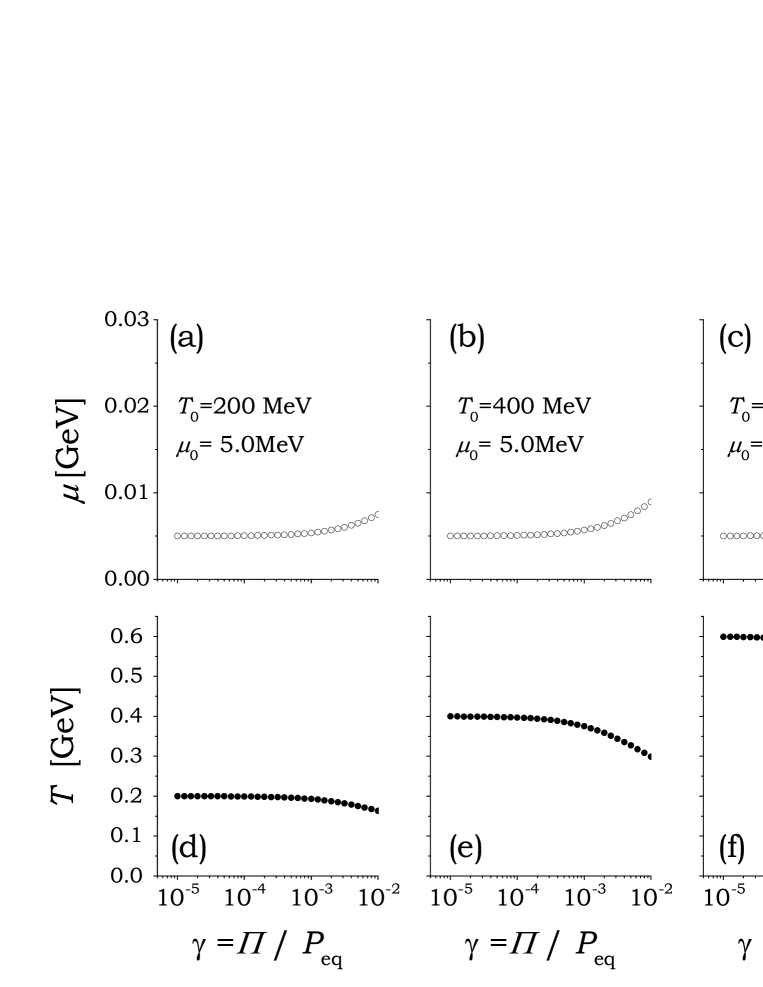
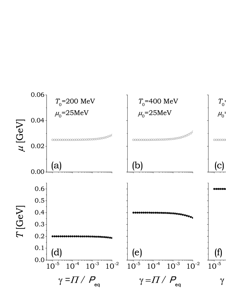
Figure 1: The separation chemical potential $\mu$ [GeV] (upper panels (a), (b), and (c)) and separation temperature $T$ [GeV] (lower panels (d), (e) and (f)) for an off-equilibrium fluid as functions of $\gamma=\Pi/P_{\rm eq}$. The $T_{0}$=0.2 GeV for figure (a) and (d), $T_{0}$=0.4 GeV, for (b) and (e), and $T_{0}$=0.6 GeV for (c) and (f), while the $\mu_{0}$=5.0 MeV is fixed for all panels.

Figure 2: The same as Fig.1 but $\mu_{0}$=25 MeV.

Figures 2 and 2 show the separation temperature $T$ and separation chemical potential $\mu$ as a function of $\gamma=\Pi/P_{\rm eq}$, $\mu_{0}$=5.0 MeV (Fig.2) and $\mu_{0}$=25 MeV (Fig.2). $T_{0}$ is fixed at 200 MeV [panels (a) and (d) of Figs.2 and 2], 400 MeV [panels (b) and (e) of Figs.2 and 2], and 600 MeV [panels (c) and (f) of Figs.2 and 2]. For very small $\gamma$ region ($\gamma\lesssim 10^{-4}$) in both Figs. 2 and 2, one can observe that $T$ and $\mu$ are almost constant with $T\approx T_{0}$ and $\mu\approx\mu_{0}$. In this region, the Landau matching condition works well. However, in the region $\gamma\gtrsim 10^{-3}$, the separation temperature $T$ decreases with increasing $\gamma$ and the separation chemical potential increases. The reason for the decrease of the separation temperature $T$ is that the total energy of the fluid is partially used in non-thermal motion such as tiny scale turbulent flow as discussed in Section 1. On the other hand, the separation chemical potential increases as $\gamma$ increases for an off-equilibrium system. This is because of the constraint of conservation of the net-baryon number, i.e., the difference between the number of particles $n_{+}$ and anti-particles $n_{-}$ must be fixed while the total number of particles and anti-particles $n_{+}+n_{-}$ decreases due to the decrease in temperature $T$.

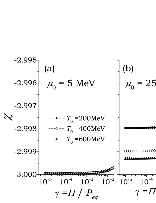
Figure 3: The $\gamma$ dependence of the factor $\chi$ eq.(56c) with the equilibrium temperature $T_{0}$=200, 400, and 600 MeV, and the equilibrium chemical potential $\mu_{0}$=5 MeV (panel (a)) and for $\mu_{0}$=25 MeV (panel (b)). In the limit of $\gamma\to 0$ and $\mu_{0}\to 0$, the $\chi$ approaches to $-3$.

Figure 3 shows the $\gamma$ dependence of the $\chi$ parameter for different $\mu_{0}$ and $T_{0}$. In the limit $\mu_{0}\to 0$ $\chi$ approaches $-3$ because $\delta\chi\to 0$. We have already reported the result $\Lambda=3\Pi$ for the baryon free case in the NeXDC correspondence PhysRevC.77.044903 , as well as the hydrodynamical model in the presence of a long-range correlation PhysRevC.81.024907 . When the strength of the off-equilibrium state $\gamma\equiv\Pi/P_{\rm eq}$ is larger than around $\sim 1/100$, the value of $\chi$ increases rapidly. This is because the bulk pressure gap between $\Pi_{+}$ and $\Pi_{-}$ becomes large in the region of $\gamma>1/100$. Recall that the parameter $\chi$ is derived from $\xi$ ($\xi=\chi\beta\Pi$), which is the residual term neglected by truncation of the energy polynomial function $P_{{\bf k}n}^{(l)}$. This means that not only quadratic, but also higher order energy dependences of both $\lambda_{\bf k}$ and $\bar{\lambda}_{\bf k}$ play an important role in the thermodynamical stability of the off-equilibrium entropy current. These higher order contributions in the energy polynomial function may result in the existence of the tiny turbulent flow in the fluid. For the finite net baryon number case, we have also obtained the same expression as given in eq.(55) PhysRevC.85.014906 ; OsadaEPJA48 . We found there that the value of $\chi$ plays an important role to restore not only the thermodynamical stability but also the causality of the solution obtained from the relativistic dissipative fluid dynamical equations. In ref.PhysRevC.85.014906 ; OsadaEPJA48 , the value of $\chi$ is introduced phenomenologically into the expression for an off-equilibrium entropy current, however, in this article, we illustrate the result numerically using kinetic theory as shown in Fig.3.

In figures 4, it is shown that the first order (scalar) correction $\lambda_{\bf k}^{*}$ to the distribution function for $\gamma=10^{-3}$ and $\gamma=10^{-2}$ with $T_{0}$ =200, 400, and 600 MeV and $\mu_{0}$=5.0 MeV. As seen in Figs.4, the off-equilibrium correction increases more rapidly in the large momentum region. This tendency is seen more explicitly as $\gamma$ increases and as the separation temperature $T$ decreases. In addition to the correction $\lambda_{\bf k}^{*}$, one need to take vector and tensor contribution, i.e., $\lambda_{\bf k}^{*\langle\mu\rangle}k_{\langle\mu\rangle}$ and $\lambda_{\bf k}^{*\langle\mu\nu\rangle}k_{\langle\mu}k_{\nu\rangle}$, respectively, into account to estimate the correction for the distribution function. However, to do this, one need set full energy-momentum tensor and net-charge current vector and this is outside the scope of the present manuscript. We plan to discuss this subject elsewhere.

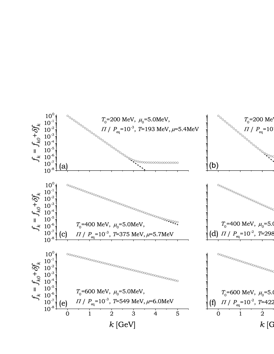
Figure 4: The off-equilibrium distribution function $f_{{\bf k}0}+\delta f_{\bf k}=(1+\lambda_{k}^{*})f_{{\bf k}0}$ for $\mu_{0}$= 5 MeV, $T_{0}$= 200 MeV (panel (a)), 400 MeV (panel (c)), and 600 MeV (panel (e)) in the case of $\gamma=10^{-3}$. The right side panels (b), (d) and (f) are the same as (a), (c) and (e), respectively, but for $\gamma=10^{-2}$. The straight line (with closed circle) is the Boltzmann distribution $f_{{\bf k}0}$ with the separation temperature $T$, and the separation chemical potential $\mu$ are shown in each panel. The open circles shows the off-equilibrium distribution function $f_{{\bf k}0}+\delta f_{\bf k}$.

4 Summary and concluding remarks

We have proposed a novel way to specify the initial conditions for a dissipative fluid dynamical model as an alternative to the so-called Landau matching condition eq.(8), employed in most of the literature published so far. The large expansion rate of matter produced in ultra-relativistic heavy-ion collisions may prevent the local equilibrium condition eq.(2) from holding true. Specifically, the microscopic collision time scale is not much shorter than any macroscopic evolution time scale because the macroscopic evolution time scale is considerably reduced due to the large gradients in thermodynamical quantities when compared to a perfect fluid. In cases characterized by eq.(5), the distribution functions are defined by eq.(6)

$$f_{\bf k}(x)=f_{{\bf k}0}[T(x),\mu(x)]+\delta f_{\bf k}(x),$$

$$\bar{f}_{\bf k}(x)=\bar{f}_{{\bf k}0}[T(x),\mu(x)]+\delta\bar{f}_{\bf k}(x).$$

For a given off-equilibrium state specified by the energy-momentum tensor given in eq.(7a) and net baryon number current defined according to eq.(7b), the Landau matching procedure equals the energy density and net baryon number density of the off-equilibrium state with those in an equilibrium of the form $T_{\rm eq}^{\mu\nu}$ and $N_{\rm eq}^{\mu}$,

$$u_{\mu}T^{\mu\nu}u_{\nu}=u_{\mu}T^{\mu\nu}_{\rm eq}u_{\nu},\quad N^{\mu}u_{\mu}=N^{\mu}_{\rm eq}u_{\mu},$$

which imposes strict restrictions on the distributions $\delta f_{\bf k}(x)$ and $\delta\bar{f}_{\bf k}(x)$. Although the physical meaning of the matching (fitting) condition is unclear, it provides the temperature $T$ and chemical potential $\mu$ for a given off-equilibrium energy density $\varepsilon=\varepsilon_{\rm eq}(T,\mu)$ and net baryon density $n=n_{\rm eq}(T,\mu)$. One may regard the Landau matching condition as just a definition for specifying an off-equilibrium state. However, it should be noted here that other off-equilibrium quantities such as the bulk pressure $\Pi$ are undoubtedly distorted by the condition. Therefore, we assert that the Landau matching condition be relaxed as shown in eq.(11),

$$\delta T^{\mu\nu}u_{\mu}u_{\nu}=\Lambda\neq 0,\quad\delta n^{\mu}u_{\mu}=\delta n\neq 0.$$

Then, $\Lambda$ and $\delta n$ obtain their entities of physical existence, i.e., they are the energy density and baryon number density of the tiny scale (less than cell size scale) disturbance flow caused by the rapid expansion of the viscous fluid.

An important consequence of the irreducible tensor expansion for the off-equilibrium distribution function is that scalar quantities such as $\Lambda$, $\delta n$, and $\Pi$ can be written as functions of the separation temperature $T$, chemical potential $\mu$, and the 0-th order scalar expansion coefficients $\lambda_{\bf k}^{*}$ (and $\bar{\lambda}_{\bf k}^{*}$). Another important consequence is that the thermodynamical stability condition requires a constraint of the scalar off-equilibrium thermodynamical quantities $\Lambda$, $\delta n$, and $\Pi$. This conditions practically determine both $\chi_{+}$ and $\chi_{-}$ (and thus also $\chi$), which are contributions neglected by the termination of polynomial function in the 0-th order irreducible tensor. By combing with the ‘equation of state’ for off-equilibrium state eq.(57), the thermodynamical stability condition eq.(55) also gives the differential equation eq.(58) for $\lambda_{\bf k}^{*}$ except for uncertainty in the integration constant $C_{\gamma}$. As seen in the solutions to the differential equations, one can observe that $\chi_{+}$ and $\chi_{-}$, which can be fixed by the thermodynamical stability condition, play an important role in the energy dependence of $\lambda_{\bf k}^{*}$. Note that, the integration constant $C_{\gamma}$ defines a scale of $\lambda_{\bf k}^{*}$, or in other words, the constant $C_{\gamma}$ regulates the ‘strength’ of the off-equilibrium state. This constant can be fixed by an index $\gamma\equiv\Pi/P_{\rm eq}$.

Although $\alpha$, $\beta$, and $\gamma$ are to be obtained as solution of eq.(76), we have investigated $\gamma$ dependence on the separation temperature $T$ and $\mu$ in a case that $u_{\mu}T^{\mu\nu}u_{\nu}$ and $N^{\mu}u_{\mu}$ are fixed and with varying $-\frac{1}{3}\Delta_{\mu\nu}T^{\mu\nu}$. In the case, the separation temperature $T$ and chemical potential $\mu$ obtained show (see Fig.2 and 2) that $T\approx T_{0}$ and $\mu\approx\mu_{0}$ hold for $\gamma<10^{-3}$. In this region, the Landau matching condition approximately holds true. However, for $\gamma>10^{-3}$, $T\neq T_{0}$ and $\mu\neq\mu_{0}$, i.e., the Landau matching condition is inappropriate and its modification is required.

In summary, although the Landau matching condition determines the matching (fitting) temperature and chemical potential by using off-equilibrium energy density and baryon number density, these are not sufficient to specify the off-equilibrium state. In this article, we have introduced an index, namely, the strength of the off-equilibrium state $\gamma\equiv\Pi/P_{\rm eq}(T,\mu)$ in order to specify the state considered more precisely. The bulk pressure $\Pi$ may relate to the disturbance flow in a fluid cell and approaches to zero when the system relaxes to the local equilibrium state. Since the fluid dynamics is a deterministic theory, to set an initial condition of the system is crucially important and it should be done very carefully. In the literature to date, a constitutive equation for the bulk pressure is solved using a likely value under the Landau matching condition ($\Lambda\equiv 0$ and $\delta n\equiv 0$). However, it must be inaccurate. The initial conditions (separation temperature $T$, chemical potential $\mu$ and bulk pressure $\Pi$) should be determined from the given off-equilibrium energy density $\varepsilon=u_{\mu}T^{\mu\nu}u_{\nu}$, net baryon number density $n=N^{\mu}u_{\mu}$, and the dissipative strength $\gamma$, as proposed in this article, i.e., eq.(76).

Appendix A Projection tensor

The deviation from equilibrium $\phi(k,x)$ can be expanded by a series of irreducible tensors, {$1$, $k^{\langle\mu\rangle}$, $k^{\langle\mu}k^{\nu\rangle}$, $k^{\langle\mu}k^{\nu}k^{\lambda\rangle}$, $\cdots$}, forming a a complete and orthogonal set. One of components of the set of irreducible tensors is defined by

$$k^{\langle\mu_{1}}k^{\mu_{2}}\cdots k^{\mu_{m}\rangle}\equiv\Delta^{\mu_{1}\mu_{2}\cdots\mu_{m}}_{\nu_{1}\nu_{2}\cdots\nu_{m}}~{}k^{\nu_{1}}k^{\nu_{2}}\cdots k^{\nu_{m}},$$ (79)

where a projection tensor, $\Delta^{\mu_{1}\mu_{2}\cdots\mu_{m}}_{\nu_{1}\nu_{2}\cdots\nu_{m}}$, is given by (See also Appendix F in Ref.PhysRevD.85.114047 )

$$\Delta^{\mu_{1},\cdots\mu_{m}}_{\nu_{1}\cdots\nu_{m}}=g_{\nu_{1}\sigma_{1}}\cdots g_{\nu_{m}\sigma_{m}}\Delta^{(\mu_{1},\cdots\mu_{m})(\sigma_{1}\cdots\sigma_{m})}\quad$$ (80a)

and

$$\Delta^{(\mu_{1},\cdots\mu_{m})(\nu_{1}\cdots\nu_{m})}\equiv\sum_{k=0}^{[m/2]}{\cal C}_{mk}~{}\Phi^{(\mu_{1}\cdots\mu_{m})(\sigma_{1}\cdots\sigma_{m})}_{mk}.$$ (80b)

The parentheses in the indexes of $\Phi^{(\mu_{1}\cdots\mu_{m})(\sigma_{1}\cdots\sigma_{m})}_{mk}$ denotes symmetrization under the exchange of indexes within $\mu_{1}\cdots\mu_{m}$ and $\sigma_{1}\cdots\sigma_{m}$ of the tensor $\Phi_{mk}$. It is written by a sum of all possible permutations of $\mu$-type and $\nu$-type indexes as follows:

$$\Phi^{(\mu_{1}\cdots\mu_{m})(\nu_{1}\cdots\nu_{m})}_{mk} \equiv \frac{1}{{\cal N}_{m,k}}\sum_{\wp_{\mu},\wp_{\nu}}\Delta^{\mu_{1}\mu_{2}}\cdots\Delta^{\mu_{2k-1}\mu_{2k}}$$ (81)

$$\quad\times\Delta^{\nu_{1}\nu_{2}}\cdots\Delta^{\nu_{2k-1}\nu_{2k}}\times\Delta^{\mu_{2k+1}\nu_{2k+1}}\cdots\Delta^{\mu_{m}\nu_{m}},$$

where $\sum_{\wp_{\mu},\wp_{\nu}}$ represents the summation of all distinct permutations of the $\mu$-type and $\nu$-type indexes. The coefficient ${\cal C}_{m,k}$ in eq.(80b) is introduced to satisfy the following conditions

$$g_{\mu_{i}\mu_{j}}\Delta^{\mu_{1}\mu_{2}\cdots\mu_{m}}_{\nu_{1}\nu_{2}\cdots\nu_{m}}=0,\quad g^{\nu_{i}\nu_{j}}\Delta^{\mu_{1}\mu_{2}\cdots\mu_{m}}_{\nu_{1}\nu_{2}\cdots\nu_{m}}=0,$$ (82)

for $1\leq i,j\leq m$. The symbol $[m/2]$ denotes the largest integer not exceeding $m/2$, and the factor ${\cal N}_{m,k}$ is the total number of distinct permutations in the indexes $\mu$ and $\nu$ to be summed. In order to consider the symmetric tensor, let us introduce the following notations for the $\mu$-type rank-2 and rank-4 tensors

$$\{\Delta^{(\mu_{i}\mu_{j})}_{m}\} \equiv \frac{1}{2}\sum_{\wp_{\mu};i,j\leq m}\Delta^{\mu_{i}\mu_{j}}=\frac{1}{2}\sum_{i}^{m}\sum_{j\neq i}^{m}\Delta^{\mu_{i}\mu_{j}},\qquad$$ (83a)

$$\{\Delta^{(\mu_{i}\mu_{j})}_{m}\}^{2} \equiv \frac{1}{2^{2}}\frac{1}{2!}\sum_{\wp_{\mu};i,j,k,l\leq m}\Delta^{\mu_{i}\mu_{j}}\Delta^{\mu_{k}\mu_{l}}$$ (83b)

$$= \frac{1}{2^{2}}\frac{1}{2!}\sum_{i}^{m}\sum_{j\neq i}^{m}\sum_{k\neq i\neq j}^{m}\sum_{l\neq i\neq j\neq k}^{m}\Delta^{\mu_{i}\mu_{j}}\Delta^{\mu_{k}\mu_{l}},$$

respectively, where the factors $\frac{1}{2}$ and $\frac{1}{2^{2}}\frac{1}{2!}$ in eq.(83a) and eq.(83b) are introduced so as to exclude duplication caused by the possible exchange of suffixes. For example, $\{\Delta^{(\mu_{i}\mu_{j})}_{m}\}^{k}$ with $m=4$ and $k=2$ means the following rank-$2k$ tensor,

$$\{\Delta^{(\mu_{i}\mu_{j})}_{4}\}^{2}=\Delta^{\mu_{1}\mu_{2}}\Delta^{\mu_{3}\mu_{4}}+\Delta^{\mu_{1}\mu_{3}}\Delta^{\mu_{2}\mu_{4}}+\Delta^{\mu_{1}\mu_{4}}\Delta^{\mu_{2}\mu_{3}}.$$

Note that, possible permutations of the suffixes include

$$\Delta^{\mu_{1}\mu_{2}}\Delta^{\mu_{4}\mu_{3}},~{}\Delta^{\mu_{2}\mu_{1}}\Delta^{\mu_{3}\mu_{4}},~{}\Delta^{\mu_{2}\mu_{1}}\Delta^{\mu_{4}\mu_{3}},$$

which gives exactly the same contribution as the above first term $\Delta^{\mu_{1}\mu_{2}}\Delta^{\mu_{3}\mu_{4}}$. In addition to this, the permutation also includes terms such as $\Delta^{\mu_{3}\mu_{4}}\Delta^{\mu_{1}\mu_{2}}$, which is also gives the same contribution. In order to exclude these terms, the factor $(\frac{1}{2})^{k}\frac{1}{k!}$ is needed. Thus, for the general $2k$-rank tensor, $\{\Delta^{(\mu_{i}\mu_{j})}_{m}\}^{k}$ ($k\leq m/2$), it is defined by

$$\{\Delta^{(\mu_{i}\mu_{j})}_{m}\}^{k} \equiv \frac{1}{2^{k}}\frac{1}{k!}\sum_{\wp_{\mu}}\Delta^{\mu_{i_{1}}\mu_{i_{2}}}\cdots\Delta^{\mu_{2k-1}\mu_{2k}},\quad$$ (84a)

where $$m \nu$$ denotes a permissible maximum number of the suffix. Similarly for -type tensors, we define

$$\{\Delta^{(\nu_{i}\nu_{j})}_{m}\}^{k} \equiv \frac{1}{2^{k}}\frac{1}{k!}\sum_{\wp_{\nu}}\Delta^{\nu_{i_{1}}\nu_{i_{2}}}\cdots\Delta^{\nu_{2k-1}\nu_{2k}}.\quad$$ (84b)

Since the tensor $\Phi^{(\mu_{1}\cdots\mu_{m})(\sigma_{1}\cdots\sigma_{m})}_{mk}$ is symmetric under permutations of both $\mu$ and $\nu-$type indexes, the last factor in the second line of eq.(81) such as $\Delta^{\mu_{2k+1}\nu_{2k+1}}\cdots\Delta^{\mu_{m}\nu_{m}}$ is different from other factors of eq.(81) denoting $\{\Delta^{(\mu_{i}\mu_{j})}_{m}\}^{k}$ and $\{\Delta^{(\nu_{i}\nu_{j})}_{m}\}^{k}$. Let us introduce a similar representation for a different symmetry as shown in the following equation;

$$\{\Delta^{\mu_{i}\nu_{j}}_{m}\}^{k}\equiv\frac{1}{k!}\sum_{\wp_{\mu}}\sum_{\wp_{\nu}}\Delta^{\mu_{i_{1}}\nu_{j_{1}}}\cdots\Delta^{\mu_{i_{k}}\nu_{j_{k}}}.$$ (85)

Then, using these definitions given in eqs.(84) and (85), we express the tensor eq.(81) as

$$\Phi^{(\mu_{1}\cdots\mu_{m})(\nu_{1}\cdots\nu_{m})}_{mk}=\frac{1}{{\cal N}_{m,k}}\{\Delta^{(\mu_{i}\mu_{j})}_{m}\}^{k}\{\Delta^{(\nu_{i}\nu_{j})}_{m}\}^{k}\{\Delta^{(\mu_{l}\nu_{l})}_{m-2k}\}^{m-2k}.$$ (86)

We hereafter denote $n^{(\mu_{i}\mu_{j})}_{m,k}$, $n^{(\nu_{i}\nu_{j})}_{m,k}$ and $n^{(\mu_{l}\nu_{l})}_{m,k}$ as the total number of distinct permutations contained in $\{\Delta^{(\mu_{i}\mu_{j})}_{m}\}^{k}$, $\{\Delta^{(\nu_{i}\nu_{j})}_{m}\}^{k}$ and $\{\Delta^{(\mu_{l}\nu_{l})}_{m}\}^{k}$, respectively. Thus, we have

$$n^{(\mu_{i}\mu_{j})}_{m,k}=n^{(\nu_{i}\nu_{j})}_{m,k}=\frac{{}_{m}P_{2k}}{k!2^{k}},$$ (87a)

$$n^{(\mu_{l}\nu_{l})}_{m,k}=\frac{[{}_{m}P_{k}]^{2}}{k!}=\frac{[m!]^{2}}{[(m-k)!]^{2}k!}.$$ (87b)

${\cal N}_{m,k}$ is the total number of possible permutations belonging to the projection tensor $\Phi^{(\mu_{1}\cdots\mu_{m})(\nu_{1}\cdots\nu_{m})}_{mk}$, which is given by

$${\cal N}_{m,k} = n^{(\mu_{i}\mu_{j})}_{m,k}~{}n^{(\nu_{i}\nu_{j})}_{m,k}~{}n^{(\mu_{l}\nu_{l})}_{m-2k,m-2k}$$ (88)

$$= \left[\frac{m!}{k!2^{k}}\right]^{2}\frac{1}{(m-2k)!}~{}.$$

Considering linear combinations for the projection tensor $\Phi^{(\mu_{1}\cdots\mu_{m})(\nu_{1}\cdots\nu_{m})}_{mk}$ with different $k$ values we obtain

$$\Delta^{(\mu_{1}\cdots\mu_{m})(\nu_{1}\cdots\nu_{m})}\equiv\sum_{k=0}^{[m/2]}\frac{{\cal C}_{m,k}}{{\cal N}_{m,k}}\{\Delta^{(\mu_{i}\mu_{j})}_{m}\}^{k}\{\Delta^{(\nu_{i}\nu_{j})}_{m}\}^{k}\{\Delta^{(\mu_{l}\nu_{l})}_{m-2k}\}^{m-2k}.\qquad$$ (89)

Note that, the value of $C_{m,0}$ can be set arbitrarily so that it may be set to the value of 1 without loss of generality. Thus, ${\cal C}_{m,k}$ can then be determined as the following:

$${\cal C}_{m,k}=(-1)^{k}~{}\frac{(m!)^{2}}{(2m)!}~{}\frac{(2m-2k)!}{k!(m-k)!(m-2k)!}~{}.$$ (90)

The derivation of eq.(90) is given in Appendix B.

Appendix B Derivation of the ${\cal C}_{m,k}$

When the indices $\mu_{1}$ and $\mu_{2}$ are expressed explicitly, the projection tensor is written as follows:

$$\Delta^{(\mu_{1}\mu_{2}\cdots\mu_{m})(\nu_{1}\cdots\nu_{m})} = \sum_{k=0}^{[m/2]}\frac{{\cal C}_{m,k}}{{\cal N}_{m,k}}\Big{[}\Delta^{\mu_{1}\mu_{2}}\{\Delta^{(\mu_{i}\mu_{j})}_{m-2}\}^{k-1}\{\Delta^{(\nu_{i}\nu_{j})}_{m}\}^{k}\{\Delta^{(\mu_{l}\nu_{l})}_{m-2k}\}^{m-2k}$$

$$\qquad+\{\Delta^{(\mu_{1}\mu_{i^{\prime}})}_{m-2}\}\{\Delta^{(\mu_{2}\mu_{j^{\prime}})}_{m-3}\}\{\Delta^{(\mu_{i}\mu_{j})}_{m-4}\}^{k-2}\{\Delta^{(\nu_{i}\nu_{j})}_{m}\}^{k}\{\Delta^{(\mu_{l}\nu_{l})}_{m-2k}\}^{m-2k}$$

$$\qquad+\{\Delta^{(\mu_{1}\mu_{i^{\prime}})}_{m-2}\}\{\Delta^{(\mu_{i}\mu_{j})}_{m-3}\}^{k-1}\{\Delta^{(\nu_{i}\nu_{j})}_{m}\}^{k}\{\Delta^{(\mu_{2}\nu_{i^{\prime}})}_{m-2k}\}\{\Delta^{(\mu_{l}\nu_{l})}_{m-2k-1}\}^{m-2k-1}$$

$$\qquad+\{\Delta^{(\mu_{2}\mu_{i^{\prime}})}_{m-2}\}\{\Delta^{(\mu_{i}\mu_{j})}_{m-3}\}^{k-1}\{\Delta^{(\nu_{i}\nu_{j})}_{m}\}^{k}\{\Delta^{(\mu_{1}\nu_{i^{\prime}})}_{m-2k}\}\{\Delta^{(\mu_{l}\nu_{l})}_{m-2k-1}\}^{m-2k-1}$$

$$\qquad+\{\Delta^{(\mu_{i}\mu_{j})}_{m-2}\}^{k}\{\Delta^{(\nu_{i}\nu_{j})}_{m}\}^{k}\{\Delta^{(\mu_{1}\nu_{i^{\prime}})}_{m-2k}\}\{\Delta^{(\mu_{2}\nu_{j^{\prime}})}_{m-2k-1}\}\{\Delta^{(\mu_{l}\nu_{l})}_{m-2k-2}\}^{m-2k-2}~{}\Big{]}.$$

Here, we take contraction of two indices $\mu_{1}$ and $\mu_{2}$ and obtain

$$g_{\mu_{1}\mu_{2}}\Delta^{(\mu_{1}\cdots\mu_{m})(\nu_{1}\cdots\nu_{m})} = \sum_{k=0}^{[m/2]}\frac{{\cal C}_{m,k}}{{\cal N}_{m,k}}\Big{[}~{}x\{\Delta^{(\mu_{i}\mu_{j})}_{m-2}\}^{k-1}\{\Delta^{(\nu_{i}\nu_{j})}_{m}\}^{k}\{\Delta^{(\mu_{l}\nu_{l})}_{m-2k}\}^{m-2k}$$ (91)

$$+c^{(1)}_{m,k}\{\Delta^{(\mu_{i}\mu_{j})}_{m-2}\}^{k-1}\{\Delta^{(\nu_{i}\nu_{j})}_{m}\}^{k}\{\Delta^{(\mu_{l}\nu_{l})}_{m-2k}\}^{m-2k}$$

$$+2c^{(2)}_{m,k}\{\Delta^{(\mu_{i}\mu_{j})}_{m-2}\}^{k-1}\{\Delta^{(\nu_{i}\nu_{j})}_{m}\}^{k}\{\Delta^{(\mu_{l}\nu_{l})}_{m-2k}\}^{m-2k}$$

$$+c^{(3)}_{m,k}\{\Delta^{(\mu_{i}\mu_{j})}_{m-2}\}^{k}\{\Delta^{(\nu_{i}\nu_{j})}_{m}\}^{k+1}\{\Delta^{(\mu_{l}\nu_{l})}_{m-2k-2}\}^{m-2(k+1)}\Big{]}=0,\quad$$

where $x\equiv g_{\mu_{1}\mu_{2}}\Delta^{\mu_{1}\mu_{2}}$ and $c^{(1)}_{mk},c^{(2)}_{mk},c^{(3)}_{mk}$ are given by

$$c^{(1)}_{m,k} = \frac{n^{(\mu_{1}\mu_{i^{\prime}})}_{m-2,1}~{}n^{(\mu_{2}\mu_{j^{\prime}})}_{m-3,1}~{}n^{(\mu_{i}\mu_{j})}_{m-4,k-2}}{n^{(\mu_{i}\mu_{j})}_{m-2,k-1}}=2k-2,\qquad$$ (92a)

$$c^{(2)}_{m,k} = \frac{n^{(\mu_{1}\mu_{i^{\prime}})}_{m-2,1}~{}n^{(\mu_{i}\mu_{j})}_{m-3,k-1}~{}n^{(\mu_{2}\nu_{i^{\prime}})}_{m-2k,1}}{n^{(\mu_{i}\mu_{j})}_{m-2,k-1}}~{}\frac{n^{(\mu_{l}\nu_{l})}_{m-2k-1,m-2k-1}}{n^{(\mu_{l}\nu_{l})}_{m-2k,m-2k}}=m-2k,\qquad$$ (92b)

$$c^{(3)}_{m,k} = \frac{n^{(\nu_{i}\nu_{j})}_{m,k}~{}n^{(\mu_{1}\nu_{i^{\prime}})}_{m-2k,1}~{}n^{(\mu_{2}\nu_{i^{\prime}})}_{m-2k-1,1}}{n^{(\nu_{i}\nu_{j})}_{m,k+1}}~{}\frac{n^{(\nu_{i}\nu_{j})}_{m-2k-2,m-2k-2}}{n^{(\mu_{i}\nu_{j})}_{m-2k-2,m-2k-2}}=2k+2.\qquad$$ (92c)

Since the contraction $g_{\mu_{1}\mu_{2}}\Delta^{(\mu_{1}\cdots\mu_{m})(\nu_{1}\cdots\nu_{m})}=0$, the coefficients $c^{(1)}_{m,k}$, $c^{(2)}_{m,k}$ and $c^{(3)}_{m,k}$ need to satisfy the following equation:

$$\frac{{\cal C}_{m,k-1}}{{\cal N}_{m,k-1}}c^{(3)}_{m,k-1}+\frac{{\cal C}_{m,k}}{{\cal N}_{m,k}}(x+c^{(1)}_{m,k}+2c^{(2)}_{m,k})=0.\quad$$ (93)

From the above equation, we obtain the following recursion formula for ${\cal C}_{m,k}$;

$${\cal C}_{m,k}=-\frac{(m-2k+2)(m-2k+1)}{2k(2m-2k+1)}~{}{\cal C}_{m,k-1}.\quad$$ (94)

Since the coefficient $C_{m,0}$ can be set to 1, ${\cal C}_{m,k}$ for general $k$ is determined according to

$${\cal C}_{m,k}=(-1)^{k}~{}\frac{(m!)^{2}}{(2m)!}~{}\frac{(2m-2k)!}{k!(m-k)!(m-2k)!}~{},$$ (95)

which is eq.(90).

Appendix C Total contraction of the projection tensor

An identity

$$g_{\mu_{1}\nu_{1}}\cdots g_{\mu_{m}\nu_{m}}\Delta^{(\mu_{1}\cdots\mu_{m})(\nu_{1}\cdots\nu_{m})}=2m+1,\qquad$$

will be used in derivation of the orthogonality condition for the irreducible projection tensors in the later Appendix D. Let us proof the identity in this section.

When the indices $\mu_{1}$ and $\nu_{1}$ are expressed explicitly, the projection tensor is written as follows:

$$\Delta^{(\mu_{1}\cdots\mu_{m})(\nu_{1}\cdots\nu_{m})} = \sum_{k=0}^{[m/2]}\frac{{\cal C}_{m,k}}{{\cal N}_{m,k}}\Big{[}\{\Delta^{(\mu_{1}\mu_{i^{\prime}})}_{m-1}\}\{\Delta^{(\mu_{i}\mu_{j})}_{m-2}\}^{k-1}\{\Delta^{(\nu_{1}\nu_{i^{\prime}})}_{m-1}\}\{\Delta^{(\nu_{i}\nu_{j})}_{m-2}\}^{k-1}\{\Delta^{(\mu_{l}\nu_{l})}_{m-2k}\}^{m-2k}$$

$$\qquad+\{\Delta^{(\mu_{i}\mu_{j})}_{m-1}\}^{k}\{\Delta^{(\nu_{1}\nu_{i^{\prime}})}_{m-1}\}\{\Delta^{(\nu_{i}\nu_{j})}_{m-2}\}^{k-1}\{\Delta^{(\mu_{1}\nu_{l^{\prime}})}_{m-2k}\}\{\Delta^{(\mu_{l}\nu_{l})}_{m-2k-1}\}^{m-2k-1}$$

$$\qquad+\{\Delta^{(\mu_{1}\mu_{i^{\prime}})}_{m-1}\}\{\Delta^{(\mu_{i}\mu_{j})}_{m-2}\}^{k-1}\{\Delta^{(\nu_{i}\nu_{j})}_{m-1}\}^{k}\{\Delta^{(\mu_{l^{\prime}}\nu_{1})}_{m-2k}\}\{\Delta^{(\mu_{l}\nu_{l})}_{\in m-2k-1}\}^{m-2k-1}$$

$$\qquad+\{\Delta^{(\mu_{i}\mu_{j})}_{m-1}\}^{k}\{\Delta^{(\nu_{i}\nu_{j})}_{m-1}\}^{k}~{}\Delta^{\mu_{1}\nu_{1}}~{}\{\Delta^{(\mu_{l}\nu_{l})}_{m-2k-1}\}^{m-2k-1}$$

$$\qquad+\{\Delta^{(\mu_{i}\mu_{j})}_{m-1}\}^{k}\{\Delta^{(\nu_{i}\nu_{j})}_{m-1}\}^{k}\{\Delta^{(\mu_{l^{\prime}}\nu_{1})}_{m-2k-1}\}\{\Delta^{(\mu_{1}\nu_{l^{\prime}})}_{m-2k-1}\}\{\Delta^{(\mu_{l}\nu_{l})}_{m-2k-2}\}^{m-2k-2}\Big{]}.$$

Contracting the indices $\mu_{1}$ and $\nu_{2}$, we get

$$g_{\mu_{1}\nu_{1}}\Delta^{(\mu_{1}\cdots\mu_{m})(\nu_{1}\cdots\nu_{m})}=\sum_{k=0}^{[m/2]}\frac{{\cal C}_{m,k}}{{\cal N}_{m,k}}\Big{[}d^{(1)}_{m,k}~{}\{\Delta^{(\mu_{i}\mu_{j})}_{m-1}\}^{k-1}\{\Delta^{(\nu_{i}\nu_{j})}_{m-1}\}^{k-1}\{\Delta^{(\mu_{l}\nu_{l})}_{m-2k+1}\}^{m-2k+1}$$

$$\quad+[d^{(2)}_{m,k}+d^{(3)}_{m,k}+xd^{(4)}_{m,k}+d^{(5)}_{m,k}]~{}\{\Delta^{(\mu_{i}\mu_{j})}_{m-1}\}^{k}\{\Delta^{(\nu_{i}\nu_{j})}_{m-1}\}^{k}\{\Delta^{(\mu_{l}\nu_{l})}_{m-2k-1}\}^{m-2k-1}\Big{]},$$ (96)

where

$$d^{(1)}_{m,k} \equiv \frac{n^{(\mu_{1}\mu_{i^{\prime}})}_{m-1,1}~{}n^{(\mu_{i}\mu_{j})}_{m-2,k-1}~{}n^{(\nu_{1}\nu_{i^{\prime}})}_{m-1,1}~{}n^{(\nu_{i}\nu_{j})}_{m-2,k-1}~{}n^{(\mu_{l}\nu_{l})}_{m-2k,m-2k}}{n^{(\mu_{i}\mu_{j})}_{m-1,k-1}~{}n^{(\nu_{i}\nu_{j})}_{m-1,k-1}~{}n^{(\mu_{l}\nu_{l})}_{m-2k+1,m-2k+1}}=m-2k+1,$$ (97a)

$$d^{(2)}_{m,k} \equiv \frac{n^{(\mu_{i}\mu_{j})}_{m-1,k}~{}n^{(\nu_{1}\nu_{i^{\prime}})}_{m-1,1}~{}n^{(\nu_{i}\nu_{j})}_{m-2,k-1}~{}n^{(\mu_{1}\nu_{l^{\prime}})}_{m-2k,1}~{}n^{(\mu_{l}\nu_{l})}_{m-2k-1,m-2k-1}}{n^{(\mu_{i}\mu_{j})}_{m-1,k}~{}n^{(\nu_{i}\nu_{j})}_{m-1,k}~{}n^{(\mu_{l}\nu_{l})}_{m-2k-1,m-2k-1}}=2k,$$ (97b)

$$d^{(3)}_{m,k} \equiv \frac{n^{(\mu_{1}\mu_{i^{\prime}})}_{m-1,1}~{}n^{(\mu_{i}\mu_{j})}_{m-2,k-1}~{}n^{(\nu_{i}\nu_{j})}_{m-1,k}~{}n^{(\mu_{i^{\prime}}\nu_{1})}_{m-2k,1}~{}n^{\mu_{l}\nu_{l}}_{m-2k-1,m-2k-1}}{n^{(\mu_{i}\mu_{j})}_{m-1,k}~{}n^{(\nu_{i}\nu_{j})}_{m-1,k}~{}n^{(\mu_{l}\nu_{l})}_{m-2k-1,m-2k-1}}=2k,$$ (97c)

$$d^{(4)}_{m,k} \equiv \frac{n^{(\mu_{i}\mu_{j})}_{m-1,k}~{}n^{(\nu_{i}\nu_{j})}_{m-1,k}~{}n^{(\mu_{l}\nu_{l})}_{m-2k-1,m-2k-1}}{n^{(\mu_{i}\mu_{j})}_{m-1,k}~{}n^{(\nu_{i}\nu_{j})}_{m-1,k}~{}n^{(\mu_{l}\nu_{l})}_{m-2k-1,m-2k-1}}=1,$$ (97d)

$$d^{(5)}_{m,k} \equiv \frac{n^{(\mu_{i}\mu_{j})}_{m-1,k}~{}n^{(\nu_{i}\nu_{j})}_{m-1,k}~{}n^{(\mu_{i^{\prime}}\nu_{1})}_{m-2k-1,1}~{}n^{(\mu_{1}\nu_{i^{\prime}})}_{m-2k-1,1}~{}n^{(\mu_{l}\nu_{l})}_{m-2k-2,m-2k-2}}{n^{(\mu_{i}\mu_{j})}_{m-1,k}~{}n^{(\nu_{i}\nu_{j})}_{m-1,k}~{}n^{(\mu_{l}\nu_{l})}_{m-2k-1,m-2k-1}}=m-2k+1.\quad$$ (97e)

Hence, we obtain a formula

$$g_{\mu_{1}\nu_{1}}\Delta^{(\mu_{1}\cdots\mu_{m})(\nu_{1}\cdots\nu_{m})}=\sum_{k=0}^{[m/2]}\gamma_{m,k}\Big{[}~{}(m-2k+1)~{}{\cal M}_{m-1,k-1}+(m+2k+2)~{}{\cal M}_{m-1,k}\Big{]},~{}$$ (98)

where

$$\gamma_{m,k} \equiv \frac{{\cal C}_{m,k}}{{\cal N}_{m,k}},$$ (99)

$${\cal M}_{m,k} \equiv \{\Delta^{(\mu_{i}\mu_{j})}_{m}\}^{k}\{\Delta^{(\nu_{i}\nu_{j})}_{m}\}^{k}\{\Delta^{(\mu_{l}\nu_{l})}_{m-2k}\}^{m-2k}.$$ (100)

This means

$$g_{\mu_{1}\nu_{1}}\Delta^{(\mu_{1}\cdots\mu_{m})(\nu_{1}\cdots\nu_{m})} = \frac{2m+1}{2m-1}\sum_{k=0}^{[m/2]-1}\gamma_{m-1,k}{\cal M}_{m-1,k}$$ (101)

$$= \frac{2m+1}{2m-1}\Delta^{(\mu_{2}\cdots\mu_{m})(\nu_{2}\cdots\nu_{m})}.$$

Using the above formula iteratively, we obtain

$$g_{\mu_{1}\nu_{1}}\cdots g_{\mu_{m}\nu_{m}}\Delta^{(\mu_{1}\cdots\mu_{m})(\nu_{1}\cdots\nu_{m})}=2m+1.\qquad$$ (102)

Appendix D Derivation of the orthogonality condition

In order to discuss the orthogonality of the irreducible projection tensor, consider the following integral for the case that $F_{\bf k}$ is an arbitrary function of $E_{k}\equiv u_{\mu}k^{\mu}$ only;

$${\cal J}_{m} = \int\!\frac{d^{3}{\bf k}~{}F_{\bf k}}{(2\pi)^{3}k^{0}}~{}k^{\langle\mu_{1}}k^{\mu_{2}}\cdots k^{\mu_{m}\rangle}k_{\langle\nu_{1}}k_{\nu_{2}}\cdots k_{\nu_{m}\rangle}$$ (103)

$$= \int\!\frac{d^{3}k~{}F_{\bf k}}{(2\pi)^{3}k^{0}}~{}[k^{\lambda}k_{\lambda}]^{m}~{}g^{\alpha_{1}}_{\beta_{1}}\cdots g^{\alpha_{m}}_{\beta_{m}}~{}\Delta^{\mu_{1}\cdots\mu_{m}}_{\alpha_{1}\cdots\alpha_{m}}~{}\Delta^{\beta_{1}\cdots\beta_{m}}_{\nu_{1}\cdots\nu_{m}}$$

$$= \Delta^{\mu_{1}\cdots\mu_{m}}_{\nu_{1}\cdots\nu_{m}}\int\!\frac{d^{3}k~{}F_{\bf k}}{(2\pi)^{3}k^{0}}~{}[k^{\lambda}k_{\lambda}]^{m}\frac{g^{\alpha_{1}}_{\beta_{1}}\cdots g^{\alpha_{m}}_{\beta_{m}}}{2m+1}\Delta^{\beta_{1}\cdots\beta_{m}}_{\alpha_{1}\cdots\alpha_{m}}$$

$$= ~{}\frac{\Delta^{\mu_{1}\cdots\mu_{m}}_{\nu_{1}\cdots\nu_{m}}}{2m+1}\int\!\frac{d^{3}k~{}F_{\bf k}}{(2\pi)^{3}k^{0}}~{}k^{\langle\alpha_{1}}\cdots k^{\alpha_{m}\rangle}k_{\langle\alpha_{1}}\cdots k_{\alpha_{m}\rangle},$$

where we require

$$\Delta^{(\mu_{1}\cdots\mu_{m})(\nu_{1}\cdots\nu_{m})}=~{}g_{\alpha_{1}\beta_{1}}\cdots g_{\alpha_{m}\beta_{m}}\Delta^{(\mu_{1}\cdots\mu_{m})(\alpha_{1}\cdots\alpha_{m})}\Delta^{(\beta_{1}\cdots\beta_{m})(\nu_{1}\cdots\nu_{m})},$$ (104)

and eq.(102). The integral part in eq.(103) can be evaluated as

$$\int\!\frac{d^{3}k~{}F_{k}}{(2\pi)^{3}k^{0}}k^{\langle\alpha_{1}}\cdots k^{\alpha_{m}\rangle}k_{\langle\alpha_{1}}\cdots k_{\alpha_{m}\rangle}=\sum_{j=0}^{[m/2]}\gamma_{m,j}\times{\cal N}_{m,j}\int\!\frac{d^{3}k~{}F_{k}}{(2\pi)^{3}k^{0}}[\Delta_{\alpha\beta}k^{\alpha}k^{\beta}]^{m}$$

$$\quad=\frac{(m!)^{2}2^{m}}{(2m)!}P_{m}(1)\int\!\frac{d^{3}k~{}F_{k}}{(2\pi)^{3}k^{0}}[\Delta_{\alpha\beta}k^{\alpha}k^{\beta}]^{m}=\frac{m!}{(2m-1)!!}~{}\int\!\frac{d^{3}k~{}F_{k}}{(2\pi)^{3}k^{0}}~{}[\Delta_{\alpha\beta}k^{\alpha}k^{\beta}]^{m},\qquad$$ (105)

where $P_{m}(x)$ is a Legendre function of the order of $m$. Hence, we can finally obtain

$$\int\!\frac{d^{3}k~{}F_{k}}{(2\pi)^{3}k^{0}}~{}k^{\langle\mu_{1}}k^{\mu_{2}}\cdots k^{\mu_{m}\rangle}k_{\langle\nu_{1}}k_{\nu_{2}}\cdots k_{\nu_{m}\rangle}~{}=\frac{m!}{(2m+1)!!}~{}\int\!\frac{d^{3}k~{}F_{k}}{(2\pi)^{3}k^{0}}[\Delta_{\alpha\beta}k^{\alpha}k^{\beta}]^{m},\qquad$$ (106)

which is eq.(15b).

Appendix E Evaluation of the $I^{(l)}_{r}$

We require to calculate the following integrals denoting $I^{(l)}_{r}$

$$I^{(l)}_{r} \equiv \int\!\frac{d^{3}{\bf k}~{}\omega^{(l)}_{\bf k}}{(2\pi)^{3}k_{0}}(E_{\bf k})^{r}$$ (107)

$$= \frac{(-1)^{l}}{2\pi^{2}}\frac{{\cal W}^{(l)}}{(2l+1)!!}\int\!\frac{k^{2}dk}{E_{\bf k}}\Big{[}\sqrt{E_{\bf k}^{2}-m^{2}}\Big{]}^{2l}~{}[E_{\bf k}]^{r}~{}e^{-(E_{k}-\mu_{\rm b})/T}.$$

This can be expressed in the following form,

$$I^{(l)}_{r} = \frac{(-1)^{l}(-1)^{r}}{2\pi^{2}}\frac{{\cal W}^{(l)}}{(2l+1)!!}~{}e^{\mu_{\rm b}/T}~{}(aT)^{2l+2+r}(\frac{d^{r}}{da^{r}})\int_{0}^{\infty}\!dy~{}[\sinh y]^{2l+2}~{}e^{-a\cosh y}$$ (108)

$$= \frac{(-1)^{l+r}}{2\pi^{2}}{\cal W}^{(l)}~{}e^{\mu_{\rm b}/T}~{}(aT)^{2l+2+r}~{}\frac{d^{r}}{da^{r}}[\frac{1}{a^{l+1}}K_{l+1}(a)],$$

where $a=m/T$. Using the identity about the following differential operators we have

$$\Big{[}\frac{d}{dz}\Big{]}^{r}=\sum_{k=0}^{[r/2]}\frac{r!}{2^{k}k!(r-2k)!}~{}z^{(r-2k)}\Big{[}\frac{1}{z}\frac{d}{dz}\Big{]}^{r-k}.$$ (109)

We then obtain

$$I^{(l)}_{r} = \frac{1}{2\pi^{2}}{\cal W}^{(l)}~{}e^{\mu_{\rm b}/T}~{}T^{2(l+1)+r}\times\sum_{k=0}^{[r/2]}\frac{(-1)^{l-k}~{}r!}{2^{k}k!(r-2k)!}~{}a^{(l+1)+r-k}K_{(l+1)+r-k}(a).\qquad$$ (110)

By requiring $I^{(l)}_{0}\equiv 1$, we can determine the normalization factor,

$$1/{\cal W}^{(l)}=\frac{(-1)^{l}}{2\pi^{2}}e^{\mu_{\rm b}/T}~{}T^{2(l+1)}~{}(\frac{m}{T})^{(l+1)}K_{(l+1)}(\frac{m}{T}).\qquad$$ (111)

Moreover, substituting the result obtained previously in the normalization factor ${\cal W}^{(l)}$, we finally obtain

$$I^{(l)}_{r} = m^{r}r!\sum_{k=0}^{[r/2]}\frac{(-1)^{k}}{2^{k}k!(r-2k)!}~{}(\frac{m}{T})^{-k}\frac{K_{l+1+r-k}(m/T)}{K_{l+1}(m/T)}.$$ (112)

Appendix F Derivation of eq.(43a)

The coefficient tensors $\lambda_{\bf k}^{\langle\mu_{1}\cdots\mu_{l}\rangle}$ and $\bar{\lambda}_{\bf k}^{\langle\mu_{1}\cdots\mu_{l}\rangle}$ must be rewritten as linear combinations of $\rho^{\mu_{1}\cdots\mu_{l}}_{m}$ or $\bar{\rho}^{\mu_{1}\cdots\mu_{l}}_{m}$ using the expressions given in eq.(41). Thus, we resubstitute eq.(41a) into the definition of $\lambda_{\bf k}$ given by eq.(37a) to yield the following expression

$$\lambda_{\bf k}^{\langle\mu_{1}\cdots\mu_{l}\rangle} = \frac{{\cal W}^{(l)}}{l!}\left(\begin{array}[]{llll}\rho_{0}^{\mu_{1}\cdots\mu_{l}},&\rho_{1}^{\mu_{1}\cdots\mu_{l}},&\cdots,&\rho_{N_{l}}^{\mu_{1}\cdots\mu_{l}}\end{array}\right)$$ (127)

$$\times\left(\begin{array}[]{llll}a^{(l)}_{00}&a^{(l)}_{10}&\ldots&a^{(l)}_{N_{l},0}\\ 0&a^{(l)}_{11}&\ldots&a^{(l)}_{N_{l},1}\\ \ldots&\ldots&\ldots&\ldots\\ 0&0&\ldots&a^{(l)}_{N_{l},N_{l}}\\ \end{array}\right)\left(\begin{array}[]{lllll}a^{(l)}_{00}&0&\ldots&0\\ a^{(l)}_{10}&a^{(l)}_{11}&\ldots&0\\ \ldots&\ldots&\ldots&0\\ a^{(l)}_{N_{l},0}&a^{(l)}_{N_{l},1}&\ldots&a^{(l)}_{N_{l},N_{l}}\\ \end{array}\right)\left(\begin{array}[]{c}E_{\bf k}^{0}\\ E_{\bf k}^{1}\\ \cdots\\ ~{}E_{\bf k}^{N_{l}}\\ \end{array}\right),\qquad$$

where we use eq.(17) in the following matrix form

$$\left(\begin{array}[]{c}P_{{\bf k}0}^{(l)}\\ P_{{\bf k}1}^{(l)}\\ \cdots\\ P_{{\bf k}n}^{(l)}\\ \end{array}\right)=\left(\begin{array}[]{lllll}a^{(l)}_{00}&0&\ldots&0\\ a^{(l)}_{10}&a^{(l)}_{11}&\ldots&0\\ \ldots&\ldots&\ldots&0\\ a^{(l)}_{N_{l},0}&a^{(l)}_{N_{l},1}&\ldots&a^{(l)}_{N_{l},N_{l}}\\ \end{array}\right)\left(\begin{array}[]{c}E_{\bf k}^{0}\\ E_{\bf k}^{1}\\ \cdots\\ ~{}E_{\bf k}^{N_{l}}\\ \end{array}\right).$$ (140)

Next, we use the following relation (see appendix G)

$$\left(\begin{array}[]{llll}a^{(l)}_{00}&a^{(l)}_{10}&\ldots&a^{(l)}_{N_{l},0}\\ 0&a^{(l)}_{11}&\ldots&a^{(l)}_{N_{l},1}\\ \ldots&\ldots&\ldots&\ldots\\ 0&0&\ldots&a^{(l)}_{N_{l},N_{l}}\\ \end{array}\right)\left(\begin{array}[]{lllll}a^{(l)}_{00}&0&\ldots&0\\ a^{(l)}_{10}&a^{(l)}_{11}&\ldots&0\\ \ldots&\ldots&\ldots&0\\ a^{(l)}_{N_{l},0}&a^{(l)}_{N_{l},1}&\ldots&a^{(l)}_{N_{l},N_{l}}\\ \end{array}\right)$$ (149)

$$\qquad=\left(\begin{array}[]{llll}I^{(l)}_{0}&I^{(l)}_{1}&\ldots&I^{(l)}_{N_{l}}\\ I^{(l)}_{1}&I^{(l)}_{2}&\ldots&I^{(l)}_{N_{l}+1}\\ \ldots&\ldots&\ldots&\ldots\\ I^{(l)}_{N_{l}}&I^{(l)}_{N_{l}+1}&\ldots&I^{(l)}_{2N_{l}}\\ \end{array}\right)^{-1},$$ (154)

which can be proved by the orthogonal condition expressed by eq.(36),

$$\sum_{k=0}^{n}I^{(l)}_{r+k}a^{(l)}_{nk}=\delta_{rn}\frac{1}{a_{nn}}.$$ (155)

Hence, we obtain

$$\lambda_{\bf k}^{\langle\mu_{1}\cdots\mu_{l}\rangle} = \frac{{\cal W}^{(l)}}{l!}\left(\begin{array}[]{llll}\rho_{0}^{\mu_{1}\cdots\mu_{l}},&\rho_{1}^{\mu_{1}\cdots\mu_{l}},&\cdots,&\rho_{N_{l}}^{\mu_{1}\cdots\mu_{l}}\end{array}\right)$$ (166)

$$\qquad\qquad\times\left(\begin{array}[]{llll}I^{(l)}_{0}&I^{(l)}_{1}&\ldots&I^{(l)}_{N_{l}}\\ I^{(l)}_{1}&I^{(l)}_{2}&\ldots&I^{(l)}_{N_{l}+1}\\ \ldots&\ldots&\ldots&\ldots\\ I^{(l)}_{N_{l}}&I^{(l)}_{N_{l}+1}&\ldots&I^{(l)}_{2N_{l}}\\ \end{array}\right)^{-1}\left(\begin{array}[]{c}E_{\bf k}^{0}\\ E_{\bf k}^{1}\\ \cdots\\ ~{}E_{\bf k}^{N_{l}}\\ \end{array}\right).$$

By integrating in whole momentum space with multiplying the weight factor $\omega_{\bf k}^{(l)}$ for the both sides of eq.(166), one obtain

$$\frac{l!}{{\cal W}^{(l)}} \int\!\!\frac{d^{3}{\bf k}~{}\omega^{(l)}_{\bf k}}{(2\pi)^{3}}\lambda_{\bf k}^{\langle\mu_{1}\cdots\mu_{l}\rangle}E_{\bf k}^{r}$$ (176)

$$= \left(\begin{array}[]{llll}\rho_{0}^{\mu_{1}\cdots\mu_{l}},&\rho_{1}^{\mu_{1}\cdots\mu_{l}},&\cdots,&\rho_{N_{l}}^{\mu_{1}\cdots\mu_{l}}\end{array}\right)\left(\begin{array}[]{llll}I^{(l)}_{0}&I^{(l)}_{1}&\ldots&I^{(l)}_{N_{l}}\\ I^{(l)}_{1}&I^{(l)}_{2}&\ldots&I^{(l)}_{N_{l}+1}\\ \ldots&\ldots&\ldots&\ldots\\ I^{(l)}_{N_{l}}&I^{(l)}_{N_{l}+1}&\ldots&I^{(l)}_{2N_{l}}\\ \end{array}\right)^{-1}\left(\begin{array}[]{l}I^{(l)}_{r}\\ I^{(l)}_{1+r}\\ \ldots\\ I^{(l)}_{N_{l}+r}\\ \end{array}\right)$$

$$= \rho_{r}^{\mu_{1}\cdots\mu_{l}},$$ (177)

because of the characteristics of the inverse matrix in eq.(177). Thus we finally obtain

$$\rho_{r}^{\mu_{1}\cdots\mu_{l}} = \!\frac{l!}{{\cal W}^{(l)}}\int\!\!\frac{d^{3}{\bf k}~{}\omega^{(l)}_{\bf k}}{(2\pi)^{3}}\lambda_{\bf k}^{\langle\mu_{1}\cdots\mu_{l}\rangle}E_{\bf k}^{r},$$ (178)

$$= \frac{l!}{(2l+1)!!}\!\int\!\frac{d^{3}{\bf k}}{(2\pi)^{3}}\lambda_{\bf k}^{\langle\mu_{1}\cdots\mu_{l}\rangle}[\Delta^{\alpha\beta}k_{\alpha}k_{\beta}]^{l}E_{\bf k}^{r}f_{{\bf k}0},$$

which is eq.(43a).

Appendix G Polynomial $P_{{\bf k}n}^{(m)}$ and its coefficients $a_{nr}^{(l)}$

The orthogonal condition of the polynomial $P_{{\bf k}n}^{(m)}$ in eq. (18) can be written in the following form

$$\left(\begin{array}[]{llllll}1&I^{(l)}_{1}&&\ldots&&I^{(l)}_{n}\\ I^{(l)}_{1}&I^{(l)}_{2}&&\ldots&&I^{(l)}_{n+1}\\ {6}\\ I^{(l)}_{n-1}&I^{(l)}_{n}&&\ldots&&I^{(l)}_{2n-1}\\ I^{(l)}_{n}&I^{(l)}_{n+1}&&\ldots&&I^{(l)}_{2n}\\ \end{array}\right)\left(\begin{array}[]{c}a^{(l)}_{n0}\\ a^{(l)}_{n1}\\ \cdots\\ a^{(l)}_{nn-1}\\ a^{(l)}_{nn}\\ \end{array}\right)=\left(\begin{array}[]{c}0\\ 0\\ \cdots\\ 0\\ 1/a^{(l)}_{nn}\\ \end{array}\right),$$ (194)

and

$$a_{nk}^{(l)}=\frac{{\cal I}^{(l)}_{nk}}{\sqrt{{\rm det}I_{n}^{(l)}{\cal I}_{nn}^{(l)}}},$$ (195)

where ${\rm det}I_{n}^{(l)}$ is the determinant of the matrix

$$\{I_{n}^{(l)}\}_{ij}=\left(\begin{array}[]{llllll}1&I^{(l)}_{1}&&\ldots&&I^{(l)}_{n}\\ I^{(l)}_{1}&I^{(l)}_{2}&&\ldots&&I^{(l)}_{n+1}\\ {6}\\ I^{(l)}_{n-1}&I^{(l)}_{n}&&\ldots&&I^{(l)}_{2n-1}\\ I^{(l)}_{n}&I^{(l)}_{n+1}&&\ldots&&I^{(l)}_{2n}\\ \end{array}\right),$$ (201)

and ${\cal I}_{nk}^{(l)}$ is a co-factor (cross out the entries that lie in the corresponding row $n$ and column $k$) of the matrix $I_{n}^{(l)}$. Thus, we can express the orthogonal function as the following

$$P_{{\bf k}n}^{(l)}=\sum_{r=0}^{N_{l}}\frac{{\cal I}^{(l)}_{nr}E_{\bf k}^{r}}{\sqrt{{\rm det}I_{n}^{(l)}{\cal I}_{nn}^{(l)}}}.$$ (202)

Then for eq.(154) we obtain, for example, in the $N_{l}=1$ case

$$\left(\begin{array}[]{cc}a_{00}^{(l)}&a_{10}^{(l)}\\ 0&a_{11}\end{array}\right)\left(\begin{array}[]{cc}a_{00}^{(l)}&0\\ a_{10}^{(l)}&a_{11}^{(l)}\end{array}\right)=\left(\begin{array}[]{cc}I_{0}^{(l)}&I_{1}^{(l)}\\ I_{1}^{(l)}&I_{2}^{(l)}\end{array}\right)^{-1}.$$ (209)

Therefore,

$$\left(\begin{array}[]{cc}a_{00}^{(l)}&a_{10}^{(l)}\\ 0&a_{11}^{(l)}\end{array}\right)\left(\begin{array}[]{cc}a_{00}^{(l)}&0\\ a_{10}^{(l)}&a_{11}^{(l)}\end{array}\right)\left(\begin{array}[]{cc}I_{0}^{(l)}&I_{1}^{(l)}\\ I_{1}^{(l)}&I_{2}^{(l)}\end{array}\right)=\left(\begin{array}[]{cc}1&0\\ 0&1\end{array}\right).\qquad$$ (218)

This is satisfied if eq.(155) holds true; i.e., for the orthogonal $0,0$ and $1,1$ components, respectively

$$((a_{00}^{(l)})^{2}+(a_{10}^{(l)})^{2})I_{0}^{(l)}+a_{10}^{(l)}a_{11}^{(l)}I_{1}^{(l)}=1+a_{10}(I_{0}a_{10}+I_{1}a_{11})\quad=1,$$ (219a)

$$a_{10}^{(l)}a_{11}^{(l)}I_{1}^{(l)}+(a_{11}^{(l)})^{2}I_{2}^{(l)}=a_{11}^{(l)}(I_{1}^{(l)}a_{10}^{(l)}+I_{2}a_{11}^{(l)})\quad=1,$$ (219b)

where we use $$a_{00}^{(l)}=1 I_{0}^{(l)}=1 0,1 1,0$$ and . However, the off-orthogonal () and () components are

$$((a_{00}^{(l)})^{2}+(a_{10}^{(l)})^{2})I_{1}+a_{10}^{(l)}a_{11}^{(l)}I_{2}^{(l)}$$

$$~{}=I_{1}^{(l)}+a_{10}^{(l)}(I_{1}^{(l)}a_{10}^{(l)}+I_{2}^{(l)}a_{11}^{(l)})=I_{1}^{(l)}+a_{10}^{(l)}/a_{11}^{(l)}$$

$$~{}=(I_{0}^{(l)}a_{10}^{(l)}+I_{1}^{(l)}a_{11}^{(l)})/a_{11}^{(l)}=0,$$ (219c)

$$a_{10}^{(l)}a_{11}^{(l)}I_{0}^{(l)}+(a_{11}^{(l)})^{2}I_{1}^{(l)}=a_{11}^{(l)}(I_{0}^{(l)}a_{10}^{(l)}+I_{1}^{(l)}a_{11}^{(l)})\quad=0,$$ (219d)

respectively.

References

- (1) Ulrich Heinz and Raimond Snellings, Ann.Rev.Nucl.Part.Sci., 63, 123–151 (2013).
- (2) Ulrich W. Heinz, J.Phys.Conf.Ser., 455, 012044 (2013).
- (3) H.A. Gustafsson, H.H. Gutbrod, B. Kolb, H. Lohner, B. Ludewigt, et al., Phys.Rev.Lett., 52, 1590–1593 (1984).
- (4) Tetsufumi Hirano, Naomi van der Kolk, and Ante Bilandzic, Lect.Notes Phys., 785, 139–178 (2010).
- (5) H. Appelshauser et al., Phys.Rev.Lett., 80, 4136–4140 (1998).
- (6) B.I. Abelev et al., Phys.Rev., C77, 054901 (2008).
- (7) A. Adare et al., Phys.Rev.Lett., 98, 162301 (2007).
- (8) B. Alver et al., Phys.Rev.Lett., 98, 242302 (2007).
- (9) Raimond Snellings, J.Phys., G41(12), 124007 (2014).
- (10) Azwinndini Muronga, Phys.Rev., C69, 034903 (2004).
- (11) Huichao Song, Steffen Bass, and Ulrich W. Heinz, Phys.Rev., C89(3), 034919 (2014).
- (12) T. Tsumura, T. Kunihiro, and K. Ohnishi, Phys.Lett., B646, 134–140 (2007).
- (13) Kyosuke Tsumura and Teiji Kunihiro, Phys.Lett., B690, 255–260 (2010).
- (14) P. Van and T.S. Biro, Dissipation flow-frames: particle, energy, thermometer, In Proceedings of the 12th Joint European Thermodynamics Conference, Cartolibreria, SNOOPY, 2013, ed. M. Pilotelli and G. P. Beretta, p546–551 (2013), arXiv:1305.3190.
- (15) Peter Arnold, Paul Romatschke, and Wilke van der Schee, JHEP, 1410, 110 (2014).
- (16) Ph. Mota, T. Kodama, R. Derradi de Souza, and J. Takahashi, Eur.Phys.J., A48, 165 (2012).
- (17) Ulrich W. Heinz, Huichao Song, and AsisK. Chaudhuri, Phys.Rev., C73, 034904 (2006).
- (18) L. D. Landau and E. M. Lifshitz, Fluid Mechanics, (Pergamon Press, 1959).
- (19) W. Israel and J. M. Stewart, Annals of Physics, 118(2), 341 – 372 (1979).
- (20) Ulrich W. Heinz, Early collective expansion: Relativistic hydrodynamics and the transport properties of QCD matter, In R. Stock, editor, ’Relativistic Heavy Ion Physics’, Landolt-Boernstein New Series, I/23. Springer Verlag, New York (2009), arXiv:0901.4355.
- (21) Carl Eckart, Phys. Rev., 58(10), 919–924 (Nov 1940).
- (22) T.S. Biro and E. Molnar, Eur.Phys.J., A48, 172 (2012).
- (23) G.S. Denicol, H. Niemi, E. Molnar, and D.H. Rischke, Phys.Rev., D85, 114047 (2012).
- (24) S.R. De Groot, W.A. Van Leeuwen, and C.G. Van Weert, Relativistic Kinetic Theory. Principles and Applications, (North-Holland, Amsterdam, 1980).
- (25) Akihiko Monnai and Tetsufumi Hirano, Phys.Rev., C80, 054906 (2009).
- (26) T. Osada, Phys.Rev., C85, 014906 (2012).
- (27) Takeshi Osada, Eur.Phys.J., A48, 167 (2012).
- (28) Larry McLerran and Michal Praszalowicz, Phys.Lett., B741, 246–251 (2015), arXiv:1407.6687.
- (29) Michal Praszalowicz, Phys.Lett., B727, 461–467 (2013), arXiv:1308.5911.
- (30) T. Osada and G. Wilk, Phys. Rev. C, 77(4), 044903 (Apr 2008).
- (31) T. Osada, Phys. Rev. C, 81(2), 024907 (Feb 2010).