A New Cepheid Distance Measurement and Method for NGC 6822

Abstract

We present a revised distance to the nearby galaxy NGC 6822 using a new multi-band fit to both previously published and new optical, near- and mid-infrared data for Cepheid variables. The new data presented in this study include multi-epoch observations obtained in 3.6 $\mu$m and 4.5 $\mu$m with the Spitzer Space Telescope taken for the Carnegie Hubble Program. We also present new observations in J, H and K_s with FourStar on the Magellan Baade telescope at Las Campanas Observatory. We determine mean magnitudes and present new period-luminosity relations in V, I, J, H, K_s, IRAC 3.6 $\mu$m and 4.5 $\mu$m . In addition to using the multi-band distance moduli to calculate extinction and a true distance, we present a new method for determining an extinction-corrected distance modulus from multi-band data with varying sample sizes. We combine the distance moduli and extinction for individual stars to determine $E(B-V)=0.35\pm 0.04$ and a true distance modulus $\mu_{o}=23.38\pm 0.02_{stat}\pm 0.04_{sys}$.

1. Introduction

As part of an ongoing mission to determine $H_{o}$ to an accuracy of 2%, the The Carnegie Hubble Program (CHP) has observed several galaxies with known Cepheid variables with the Spitzer Space Telescope (Freedman et al., 2011). These warm mission data includes multi-epoch observations with the Infrared Array Camera (IRAC) in the 3.6 $\mu$m and 4.5 $\mu$m passbands (Channels 1 and 2). In this paper we present a Cepheid distance analysis of the local dwarf irregular galaxy NGC 6822 using these new data, as well as new near-IR ground based observations and previously published visible and near-IR data.

Building upon the discovery of variables in NGC 6822 and the first step in the distance scale beyond the Magellanic Clouds by Hubble (1925), the definitive study of the Cepheid population was that of Kayser (1967). She acquired photographic B and V photometry for 13 Cepheids with periods ranging from 10 to 90 days and measured a distance modulus $\mu_{o}=23.75$ mag and a relatively high reddening of $E(B-V)=0.27$ mag. Subsequent re-observation and analysis of these Cepheids proceeded apace, including a near-IR H-band study by McAlary et al. (1983) who found $\mu_{o}=23.47\pm 0.11$, with less sensitivity to the high extinction of NGC 6822. More recent multi-band studies have narrowed the range of Cepheid distances and better constrained the average and differential reddening (Gallart et al., 1996; Pietrzyński et al., 2004; Gieren et al., 2006; Feast et al., 2012).

NGC 6822 lies at a low galactic latitude ($b\sim-$18°) and thus suffers a large line of sight extinction, with derived reddening values varying from $E(B-V)$ of 0.19 to 0.42 mag (Gallart et al., 1996). This makes it a prime target for the use of near and mid-IR observations for distance determination. With the accurate calibration of the Cepheid distance ladder using Spitzer IRAC data, including well-constrained galactic and Large Magellanic Cloud period-luminosity (PL) relations and distances, we are poised to examine the Cepheids in NGC 6822 at mid-IR wavelengths (Scowcroft et al., 2011; Freedman et al., 2011; Monson et al., 2012).

A previous study of archival, single-epoch observations of Cepheids in NGC 6822 by Madore et al. (2009) provided motivation and proof-of-concept for the use of IRAC data in measuring the PL relations despite the potential for crowding and high stellar background at mid-IR wavelengths. Recent near-IR studies by Gieren et al. (2006) and Feast et al. (2012) (henceforth F12) still indicate some uncertainty in the Cepheid distance, even when compared against the previous Spitzer data. We discuss this discrepancy and its possible causes.

In this study we follow up on the single epoch data with new 12 epoch Spitzer IRAC observations which are used to determine more accurate mid-IR mean magnitudes. We also investigate the calculation of the reddening and true distance modulus with multi-wavelength fits, combining multiple datasets. Our sample has been compiled from the OGLE and Araucaria projects, which have of V, I, J and K_s observations of a large number of Cepheids i(Pietrzyński et al., 2004; Gieren et al., 2006).

When multi-wavelength fitting of a reddening law to apparent distance moduli of Cepheids in external galaxies was first undertaken (Freedman et al. 1985; Freedman 1985, 1988; Freedman et al. 1991) its efficacy and novelty largely outweighed its rigorous and self-consistent application. Distance moduli of individual stars in the galaxy were assumed to be representative, and to be unbiased with respect to one another. As the amount of observations useful for such an analysis grows the method can be refined with an increasing number of passbands to better constrain the line-of-sight extinction and thus the true distance, but for a variety of technical reasons (field of view, detector types, etc.) the stars observed often represent different samplings of the instability strip and individually different line-of-sight extinction. This can lead to a situation where one derives an average reddening and true distance with datasets which may or may not suffer from systematic bias due to different samplings of the instability strip or regions of the galaxy (and thus different reddenings) for each passband used.

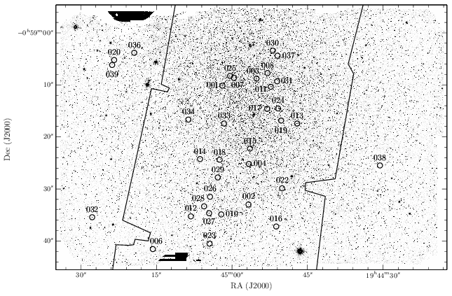
Figure 1.— J-Band image of NGC 6822 created from our FourStar data with the overlapping Spitzer IRAC field of view overlaid with black lines. The total Spitzer IRAC field of view extends beyond the northern and southern edges of the FourStar field of view. Cepheids that fall within the FourStar field of view are marked with circles.

To remedy the resulting bias new methodologies need to be explored. One possibility is to keep the basic approach the same, but limit the analysis to a very restricted sample of Cepheids containing (say) only those stars that have data at all of the considered wavelengths, and/or completely dropping from the analysis wavelengths that have the smallest number of observations. The first-suggested, sample restricted approach was recently adopted by F12 in their analysis of Cepheid data for NGC 6822. While minimizing systematic effects of incoherent samples, the downside of this approach is that large numbers of stars or wavelengths drop out of the analysis and stop contributing to the solution. Some, often hard-won, information is inevitably lost; the trade-off being sample-size reduction (decreased precision) for increased accuracy (decreased bias).

In this paper, we present a new method for determining extinction and true distance modulus using samples of varying sizes and compositions at multiple wavelengths. Following the discussion of Freedman et al. (1991), we calculate individual distance moduli for each Cepheid and use the results to generate a true distance modulus gaussian mixture distribution. With our method we hope to bypass some of the possible biases introduced in choosing which Cepheids to use in defining a PL relation. Throughout this paper we adopt a distance to the LMC of $\mu_{o}=18.477\pm 0.033$ (Freedman et al. 2012; Monson et al. 2012) and the Cepheid PL relations used in Scowcroft et al. (2013), derived by Fouqué et al. (2007) for the V & I bands, Persson et al. (2004) for the J, H & K_s bands and Scowcroft et al. (2011); Monson et al. (2012) for the IRAC 3.6$\mu$m & 4.5$\mu$m data.

2. Sample, Observations and Reduction

In this paper we use both previously published as well as new observations. To compose our sample of Cepheids, we refer to the work of Pietrzyński et al. (2004), which includes coordinates and the most up-to-date list of Cepheids in NGC 6822, including the re-discovery of Cepheids previously observed with both photographic plates and CCDs (Hubble 1925; Kayser 1967; McAlary et al. 1983; Gallart et al. 1996; Antonello et al. 2002). To simplify matters, we refer to the stars used in our analysis by the unique identifier given in Pietrzyński et al. (2004) and adopt the periods determined with their well-sampled data. We restrict our analysis to Cepheids with a periods greater than 6 days, resulting in 39 stars. Their positions are shown in Figure 1, a list of the Cepheids with new observations presented in this work is given in Table 1, and a list of all the Cepheids used for our analysis is given in Table 2. Where observations have already been published, we do not re-reduce or re-photometer the existing data. An example of the phased data points is shown in Figure 2 and the remaining Cepheid data plots are given in the Appendix.

Table 1New Spitzer & FourStar Photometry

Name	$passband$	mag.	$\sigma$	MJD
CEP001	[3.6]	14.44	0.05	55137.1
CEP001	[3.6]	14.44	0.04	55151.0
CEP001	[3.6]	14.40	0.06	55159.5
CEP001	[3.6]	14.62	0.04	55168.6
CEP001	[3.6]	14.61	0.03	55345.5
CEP001	[3.6]	14.56	0.03	55359.3
CEP001	[3.6]	14.48	0.05	55367.5
CEP001	[3.6]	14.38	0.03	55376.5
CEP001	[3.6]	14.41	0.05	55512.4
CEP001	[3.6]	14.55	0.05	55526.2
CEP001	[3.6]	14.59	0.04	55535.2
CEP001	[3.6]	14.69	0.04	55544.7

Multi-epoch photometry of Cepheids measured from our new Spitzer and FourStar data. Table 1 is published in its entirety in the electronic edition of ApJ. A portion is shown here for guidance regarding its form and content.

Figure 2.— Light curve photometry for a typical Cepheid from our sample. The average magnitude and its error are calculated using the GLOESS fits, shown in this plot as the continuous lines. In cases where the data were not well-sampled, J, H or K_s magnitudes are not plotted and were calculated by finding the average value of the data points (see Table 2). The FourStar data, plotted as stars, agree well with those of F12, as discussed in section 2.4. In all cases the J, H and K_s fits are dominated by the F12 data. Error bars have been omitted for clarity; they are listed in Table 1.

Table 2Mean Magnitudes

Cepheid ID	P (Days)	V($\sigma$)	I($\sigma$)	J($\sigma)$	H($\sigma$)	Ks($\sigma$)	[3.6]($\sigma$)	[4.5]($\sigma$)	Notes
CEP001	123.90	17.90(03)	16.48(03)	15.61(05)	15.14(05)	14.95(05)	14.56(04)	14.52(04)	b
CEP002	65.320	17.69(03)	16.44(02)	15.62(03)	15.16(02)	15.00(02)	14.90(02)	14.87(03)	b
CEP003	37.461	18.69(04)	17.38(03)	16.55(03)	16.04(03)	15.91(03)	15.56(04)	15.63(04)	a
CEP004	34.663	18.92(04)	17.60(03)	16.77(03)	16.26(03)	16.13(02)	15.88(05)	15.99(05)	a
CEP005	32.419	18.87(03)	17.68(02)	…	…	…	…	…
CEP006	31.868	18.63(05)	17.42(03)	16.58(02)	16.11(01)	16.05(01)	15.82(03)	…	d,e
CEP007	30.512	19.08(05)	17.76(03)	16.84(03)	16.34(03)	16.18(04)	15.85(04)	15.92(03)	a
CEP008	29.211	19.25(04)	17.95(03)	16.94(02)	16.38(01)	16.36(01)	16.01(03)	16.15(03)	d
CEP009	21.120	19.45(04)	18.29(02)	…	…	…	…	…
CEP010	19.960	19.52(04)	18.27(03)	17.51(04)	17.03(04)	16.90(04)	16.72(03)	16.75(02)	a
CEP011	19.887	19.90(03)	18.53(02)	17.61(03)	17.04(03)	16.94(05)	16.85(03)	16.86(03)	a
CEP012	19.602	19.79(03)	18.47(02)	17.68(02)	17.14(02)	17.04(02)	16.85(04)	16.90(02)	a
CEP013	19.295	19.76(04)	18.61(03)	…	…	…	…	…
CEP014	18.339	19.59(04)	18.35(03)	17.59(02)	17.13(02)	17.01(03)	16.75(04)	16.81(05)	a
CEP015	17.344	19.54(04)	18.38(03)	17.67(02)	17.23(02)	17.11(02)	16.66(02)	16.74(02)	a
CEP016	16.960	19.91(04)	18.71(02)	17.88(03)	17.38(04)	17.23(04)	17.01(04)	16.88(02)	a,e
CEP017	16.855	20.15(03)	18.79(02)	17.89(02)	17.31(02)	17.23(04)	16.83(02)	16.90(02)	a
CEP018	13.872	19.92(03)	18.68(02)	17.95(02)	17.51(02)	17.31(02)	17.01(02)	17.07(04)	a
CEP019	11.164	19.99(02)	18.83(01)	17.99(03)	17.49(02)	17.49(02)	17.00(01)	17.17(01)	d
CEP020	10.925	19.55(03)	18.69(02)	17.96(02)	17.58(01)	17.60(01)	…	…	d
CEP021	10.783	19.91(04)	18.91(02)	…	…	…	…	…
CEP022	10.277	20.56(02)	19.39(02)	18.45(08)	17.98(05)	18.03(06)	…	…	c
CEP023	9.5731	20.24(04)	19.14(02)	…	…	…	17.74(04)	…
CEP024	9.3664	20.49(04)	19.27(02)	18.45(09)	17.98(06)	18.04(06)	…	…	c
CEP025	8.9367	20.94(02)	19.24(01)	18.14(02)	17.42(02)	17.18(02)	…	…	a,f
CEP026	8.4670	20.27(03)	19.14(02)	18.51(03)	18.04(01)	17.90(03)	17.63(02)	17.70(01)	a,g
CEP027	8.3912	20.58(03)	19.39(02)	…	…	…	17.63(01)	17.65(02)
CEP028	7.2085	19.93(02)	18.53(01)	17.52(02)	16.89(01)	16.71(02)	…	…	a,g
CEP029	7.1054	20.94(03)	19.75(01)	…	…	…	…	…	g
CEP030	6.8842	20.98(03)	19.79(02)	…	…	…	…	…
CEP031	6.8665	20.86(04)	19.73(02)	…	…	…	…	…
CEP032	6.7650	20.74(02)	19.75(02)	…	…	…	…	…
CEP033	6.7356	20.97(03)	19.69(02)	…	…	…	…	…
CEP034	6.5391	20.76(03)	19.55(02)	…	…	…	…	…
CEP035	6.2965	20.78(03)	19.67(02)	…	…	…	…	…
CEP036	6.1457	20.58(02)	19.63(01)	…	…	…	…	…
CEP037	6.1387	21.10(03)	20.03(02)	…	…	…	…	…
CEP038	6.0637	20.95(04)	19.84(02)	…	…	…	…	…
CEP039	6.0011	20.72(03)	19.73(02)	…	…	…	…	…

Cepheid ID and periods for all Cepheids with periods greater than 6 days from (Pietrzyński et al., 2004)
(a) F12 and FourStar data used in Gloess fit
(b) F12 data only used in Gloess fit, FourStar data excluded due to phase shifting
(c) F12 and FourStar data averaged to determine mean magnitude
(d) No F12 data available, FourStar data only averaged to determine mean magnitude
(e) Spitzer cold data excluded from Gloess fit due to phase shifting
(f) Star excluded from further analysis due to crowding (See Figure A.1)
(g) Star excluded from further analysis due to deviation from PL relations (Pietrzyński et al., 2004; Gieren et al., 2006)

2.1. Warm Spitzer Observations

New mid-infrared observations of NGC 6822 were taken during the Warm Spitzer mission as part of a larger survey of Cepheids in external galaxies (PID 61001). Data were taken for twelve separate epochs from November 2009 to December 2010. The data were taken with IRAC at 3.6 $\mu$m and 4.5 $\mu$m, with frame times of 30 s. Both IRAC channels were observed simultaneously and the total area covered by the Spitzer observations forms a rectangle roughly 0.15° by 0.45° centered on the galaxy, with the long axis aligned roughly 12 degrees west of north. The field covered in all 12 epochs corresponds to a subset of the rectangle centered on the galaxy approximately 0.11° by 0.23°. Due to the 1.2′ offset in the FOV of the 3.6 $\mu$m channel from the 4.5 $\mu$m channel and the rotation of the spacecraft throughout the year, the number of epochs a star is observed can vary from 4 to 8 in the outer regions of the field to 12 epochs in the main portion (see, e.g., Scowcroft et al. 2013).

The data reduction and analysis follow the same steps described in detail in Scowcroft et al. (2013). In short, a time-averaged mosaic is created from all 12 epochs to build a deep picture of the field. For the brighter stars, individual epoch mosaics are then used to measure the light curves. For the fainter stars, the deep frame is used for producing an average photometric magnitude. Photometry was carried out with DAOPHOT and ALLFRAME (Stetson 1987, 1994) on both the time-averaged mosaics and the single-epoch mosaics. DAOPHOT was used initially to create a PSF model and object catalog, while final photometry was performed using ALLFRAME. A model PSF for each mosaic was generated using bright, unsaturated, uncrowded stars and allowed to vary in a linear fashion across the field of view. To determine the accuracy of the photometry thousands of artificial stars were added in a grid to each mosaic and the photometry was rerun several times, shifting the grid in a systematic fashion with each subsequent re-run. Artificial star tests resulted in recovery of greater than 95% of artificial stars down to ${\sim}17.5$ mag at ${\sim}$0.1 mag photometric accuracy. Our Spitzer photometry is calibrated using the standard system of Reach et al. (2005).

2.2. Cold Spitzer Data

We include in this analysis archival, single-epoch observations taken prior to the end of the cryogenic mission by the SINGS survey (Kennicutt et al., 2003). Photometry of the Cepheids from those observations was first presented by Madore et al. (2009), who showed the utility of even single-epoch data for determining mid-IR mean magnitudes for the low amplitude light curves encountered even for luminous Cepheids. Taken together with the new warm Spitzer data, the Cepheids in our sample have up to 13 individual epochs. Mean magnitudes should therefore be well determined even for the faintest stars, whose light curves cannot be delineated.

2.3. FourStar Observations

NGC 6822 was imaged with the FourStar Infrared Camera (Persson et al., 2013) on the 6.5 m Baade telescope at Las Campanas Observatory. The J, H and K_s observations were made on the nights of May 7, 11, 28 2012; the median seeing was 0.45, 0.7, 1.1″FWHM respectively. The FourStar field of view is 11’$\times$11’ (4 detectors with 18″ gaps and a pixel scale of 0.159″/pixel) allowing most of NGC 6822 (5’$\times$11’) to fit onto two detectors. A 2-position beam-switching technique was used to measure the sky background. In the A-position NGC 6822 is placed on detectors 1 and 2 (aligned N-S) with sky on detectors 3 and 4 (also N-S). In the B-position, NGC 6822 is placed on detectors 3 and 4 with the sky on detectors 1 and 2. A nine-position dither pattern was used at each beam position to mitigate array artifacts and cosmic rays. Final exposure times were 2.1, 2.2 and 3.8 hours at J, H and K_s respectively.

Photometry of stars in the resulting 9 FourStar mosaics (three bands for each epoch) was performed using DAOPHOT (Stetson, 1987). star tests were carried out in the same manner as described in section 2.1. The artificial stars were accurately recovered brighter than roughly 19th magnitude in J, H and K_s, with an accuracy in the photometry of approximately 10% at the faint end increasing to 1% at the bright end (${\sim}$13th mag), except for the May 7 observations where the accuracy is about a factor of two less due to marginal sampling caused by excellent seeing.

The JH_s photometry was calibrated to the 2MASS system (using 2MASS stars in the NGC 6822 field itself) for the nights of May 11 and 28. The excellent seeing for the May 7 observations was such that the number of unsaturated stars in the image that match those in the 2MASS catalog was too few and too inaccurate to calculate a calibration. The zero point offset from 2MASS for May 7 was therefore calculated by comparing unsaturated stars from the May 7th catalog to the 2MASS calibrated May 11th catalog.

2.4. Previously Published near-IR Observations

Extensive J, H and K_s observations were done by F12 using the SIRIUS camera on the Infrared Survey Facility Telescope at the South African Astronomical Observatory. These data cover 16 to 19 epochs, thus sampling the Cepheid light curves extremely well. Gieren et al. (2006) obtained two to four epochs of J and K_s observations using the PANIC and SOFI instruments at Las Campanas and La Silla, respectively. F12 noted systematic discrepancies between their measured magnitudes and those of Gieren et al. (2006), though they did not determine a cause. These discrepancies, which amount to mean differences of 0.126$\pm$0.022 mag in J and 0.061$\pm$0.014 mag in K_s, are not only major, but lead to unaccounted for differences in the derived distance moduli. They should therefore be cleared up.

One possible cause of the discrepancies is the photometric calibration applied to each dataset: F12 use 2MASS stars within the field to calibrate their data, as shown in F12. Gieren et al. (2006) use separate observations of standard stars to put their data on the UKIRT system, then transform that data to the Persson et al. (2004) system, which is virtually identical to the 2MASS system (Carpenter, 2001). Thus system transformations don’t seem relevant to the problem above perhaps a few hundredths of a magnitude. Another possibility lies in the different methods used to calculate mean magnitudes: F12 used Fourier-fits, while Gieren et al. (2006) determine a mean magnitude from one to three individual observations using the template fitting method of Soszyński et al. (2005). Phasing problems should not be an issue in the latter method, because the Gieren et al. (2006) and Soszyński et al. (2005) data were acquired nearly contemporaneously.

The F12 data sample the light curves much better than do our new FourStar data, and the latter cannot materially improve the F12 mean magnitudes. Nevertheless, the FourStar data are important in deciding which of the two published datasets – F12 or Gieren et al. (2006) – is correct. We first did GLOESS fits to the F12 light curve data. We then examined the differences between our individual data points and that of the fitted F12 data, on a point-by-point basis. This was done only in those cases where the F12 phase coverage in the neighborhood of the FourStar data points was sufficient to allow a reasonable local GLOESS fit in principle (noise is another matter). The average differences, in the sense FourStar minus F12, are $-0.03\pm 0.06$ (10, 21), $-0.02\pm 0.05$ (10, 21), and $0.01\pm 0.07$ (9,16), in J, H, and K_s, respectively, where the error bars are the dispersions, and the numbers in parentheses are the numbers of stars and comparison points respectively. The rather large scatters in the differences arise mostly from cases in which the F12 data themselves scatter around the fitted light curves, thus leading to uncertain fits. The average differences and their uncertainties ( $\sim$ 0.0.014 mag) are small enough, however, to decisively favor the F12 data over the Gieren et al. (2006) data. Our final mean magnitudes were found by inserting the FourStar data directly into the F12 light curves (with no transformations) and using GLOESS to produce the values in Table 2.

2.5. Previously Published Optical Data

We do not present any new optical data in this paper, but we do make use of published V and I-band data obtained with the Warsaw 1.3 m telescope at Las Campanas Observatory over 77 nights in 2002. These well-sampled data, taken as part of the OGLE survey and Araucaria projects, were presented by Pietrzyński et al. (2004).

3. Results

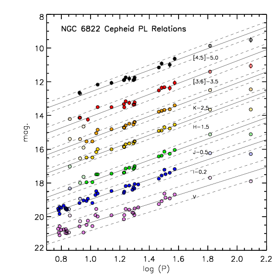
Figure 3.— Period-Luminosity relations in all of the bands used in this paper; data are in Table 1. The solid lines represent the unweighted least-squares fits and the dashed lines show the $\pm$2-$\sigma$ deviations. The open symbols are not used in the fitting. Magnitudes are uncorrected for extinction.

3.1. Average Magnitude Determination

We have re-determined the mean magnitudes in all of the passbands used, including data from the literature. This includes the individual epoch V and I data from Pietrzyński et al. (2004), J, H and K_s data from F12 (including the FourStar data, and the new multi-epoch IRAC data with a single point added to the light curves where applicable from Madore et al. (2009). Where possible, we have fitted smooth light curves using the GLOESS program (Persson et al. 2004). For the V and I-band data we decrease and increase the width of the gaussian smoothing window where the data are well sampled and less well sampled, respectively. The mean magnitudes that we measure for V and I respectively are, on average, fainter than the means calculated by Pietrzyński et al. (2004) by $0.03\pm 0.02$ and $0.01\pm 0.01$ mag. Our J, H and K_s mean magnitudes are fainter than those found in F12 by $0.01\pm 0.02$, $0.00\pm 0.01$ and $0.01\pm 0.01$ respectively.

An example of the resulting light curve fits to the data in all available passbands is shown in Figure 2; the remaining fits are given in the Appendix. We omit the FourStar data from the light curves of CEP001 and CEP002 as there appears to be some phase shifting. The Madore et al. (2009) data for CEP006 and CEP016 do not phase well with the new warm Spitzer data and have also been omitted from the light curve fit. The mean magnitudes and errors are determined from the light curve fits with GLOESS and are listed in Table 2. The total error in each band is a combination of the systematic (i.e., from fitting) and random photometric errors. As the data are randomly sampled, the photometric error decreases as $1/\sqrt{N}$, where N is the total number of independent observations in each passband.

Of the 22 stars in our sample with J, H and K_s photometry, four were not measured by F12. For these, the FourStar data are not sufficient to fit light curves. In a study of IC 1613, Scowcroft et al. (2013) determined that the shifts in the period and phase over time lead to inaccuracies in template fitting to their FourStar data points. They therefore adopt mean magnitudes and errors by simply averaging the available data points. We do the same for the stars in our sample which lack sufficient near-IR data to fit a light curve: mean magnitudes and their errors are noted in Table 2. Note that the J, H and K_s magnitudes derived from GLOESS fits are dominated primarily by the F12 data, as our FourStar observations only add two to three data points to the curves (e.g. Fig. 2). Of the 22 stars in our sample with J, H and K_s magnitudes, only four were not measured by F12.

Table 3PL Relation Slopes and Zero Points

band	Slope (a)	Slope (a)	Zero-point (b)	Zero-point (b)	N
	fitted	literature	NGC 6822	LMC
V	-2.65	-2.734	23.08	14.318	34
I	-2.89	-2.957	22.14	13.632	34
J	-3.03	-3.153	21.56	13.183	17
H	-3.14	-3.234	21.17	12.845	17
Ks	-3.27	-3.281	21.15	12.770	17
$[3.6]$	-3.14	-3.31	20.86	12.70	16
$[4.5]$	-2.91	-3.21	20.79	12.69	14

We derive distance moduli by fixing our slope to the literature values in column 2. The references are for V & I Fouqué et al. 2007; for J, H & K_s: Persson et al. 2004; for $[3.6]$ & $[4.5]$: Scowcroft et al. 2011; Monson et al. 2012. The number of stars used in each fit is given in column 6.

3.2. Period-Luminosity Relations

To determine the PL relation in each passband we use the largest possible sample of mean magnitudes for each color and fit only stars with periods between 6 and 60 days. Following the discussion of Pietrzyński et al. (2004) and Gieren et al. (2006), we reject CEP026, CEP028 and CEP029 from the V, I, J, H and K_s fits due to their distance from the mean PL relation in those studies and CEP025 from the J, H and K_s fits due to crowding (see Table 2). The PL relations take the form:

$$M_{\lambda}=a_{\lambda}(\log P-1.0)+b_{\lambda}$$

An unweighted least-squares fit is performed to each passband; the resulting fit PL relations for each pass-band are shown in Figure 3. The slopes and zero points that we derive are given in Table 3.

4. Distance Determinations to NGC 6822

A low galactic latitude leads to a large extinction along the line of sight to NGC 6822, extinction within the galaxy itself, and variable extinction across its face (Fusco et al., 2012). It is thus of particular importance to solve for the extinction with high accuracy. Reddening-insensitive Wesenheit magnitudes (Madore 1976, 1982) can be calculated using two optical passbands, as in Pietrzyński et al. (2004), resulting in a lower dispersion PL relation and a more accurate extinction-free distance. Alternatively, a distance modulus can be measured for each observed passband and a reddening law fit to the individual distance moduli for each passband, resulting in an extinction-corrected true distance modulus. Gallart et al. (1996) present BVRI photometry of six Cepheids outlining the utility of this method and the importance of using an appropriate reddening law (Gieren et al., 2006; Madore et al., 2009; Feast et al., 2012). The latter method uses all the available data, and with the addition of [3.6 $\mu$m] whould give a more robust solution with less extrapolation.

4.1. Distance and Extinction of the Ensemble

In this method we use the adopted slope solutions $a_{\lambda}$ given in Table 3 and find $b_{\lambda}$. Offsets of $b_{\lambda}$ with respect to those for the LMC give the apparent distance moduli for each passband, under our assumption that the true (reddening-corrected) distance modulus of the LMC is 18.477$\pm$0.033 mag. Table 4 lists these apparent distance moduli and Figure 4 plots them against $\lambda^{-1}$. The curve is a weighted least-squares fit assuming a Cardelli et al. (1989) reddening law with a fixed R${}_{v}=3.1$. To account for the varying samples and sets, we estimated the statistical errors in the distance moduli by performing the fit for each band 5000 times while resampling the population with both a random number of objects and a random shift in the measured magnitude within the assigned error bar. The final error is derived from a gaussian fit to the resulting distribution of moduli. We then apply the reddening law of Cardelli et al. (1989) to the apparent moduli to determine a true distance modulus $\mu_{o}$ = 23.38$\pm$0.05 and extinction $E(B-V)$ = 0.36$\pm$0.09. We exclude the Spitzer 4.5 $\mu$m band from our final $\mu_{o}$ calculation both here and in our subsequent analyses and discussion; in previous studies the 4.5 $\mu$m band was found to be contaminated by the CO band-head at 4.6 $\mu$m (Freedman et al., 2011; Scowcroft et al., 2011; Monson et al., 2012).

Table 4Individual Passband Observed Distance Moduli

	V	I	J	H	Ks	[3.6]	[4.5]
$\mu$	24.51	24.03	23.71	23.59	23.56	23.35	23.38
$\sigma$	0.08	0.05	0.09	0.08	0.07	0.09	0.08

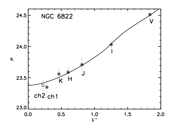
Figure 4.— First method for calculating a true distance modulus, $\mu_{o}$ and $E(B-V)$. Data points correspond to the distance modulus from each band plotted as a function of inverse wavelength, $\lambda^{-1}$. A reddening law fit to the moduli (excluding 4.5$\mu$m ) is plotted as the solid line. The Cardelli et al. (1989) reddening law was used with a fixed R${}_{v}=3.1$ and $E(B-V)$ and $\mu_{o}$ allowed to vary. The resulting fit provides an extinction-corrected distance modulus of 23.38$\pm$0.05 mag and $E(B-V)$ = 0.36$\pm$0.09.

4.2. Distances and Extinctions of Individual Cepheids

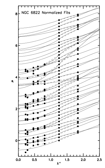
Figure 5.— Individual reddening fits applied to each Cepheid, normalized to each star’s I-band magnitude and offset from one another by an arbitrary constant amount for plotting purposes. The fits to all 39 Cepheids are shown, increasing in period from CEP039 at the top to CEP001 at the bottom.

Table 5Derived Individual passband $\mu$ and Fit Values

Name	$\mu_{V}$	$\mu_{I}$	$\mu_{J}$	$\mu_{H}$	$\mu_{K_{s}}$	$\mu_{3.6}$	$\mu_{4.5}$	$\mu_{o}$	$\sigma$	AV	$\sigma$
CEP001	25.05	24.56	24.35	24.31	24.24	23.96	23.81	23.96	0.02	1.07	0.04
CEP002	24.08	23.69	23.48	23.42	23.38	23.38	23.27	23.28	0.01	0.74	0.03
CEP003	24.41	23.92	23.65	23.53	23.49	23.24	23.26	23.30	0.02	1.09	0.04
CEP004	24.55	24.04	23.76	23.65	23.61	23.44	23.51	23.46	0.02	1.03	0.04
CEP005	24.43	24.04	…	…	…	…	…	23.46	0.08	0.96	0.10
CEP006	24.17	23.75	23.53	23.46	23.53	23.27	…	23.38	0.01	0.67	0.04
CEP007	24.57	24.04	23.71	23.59	23.52	23.23	23.26	23.26	0.02	1.31	0.04
CEP008	24.68	24.17	23.69	23.55	23.51	23.33	23.43	23.35	0.01	1.28	0.03
CEP009	24.50	24.10	…	…	…	…	…	23.51	0.08	0.98	0.10
CEP010	24.50	24.00	23.74	23.63	23.58	23.49	23.50	23.45	0.02	0.97	0.04
CEP011	24.88	24.26	23.85	23.65	23.58	23.61	23.61	23.48	0.02	1.33	0.03
CEP012	24.75	24.18	23.88	23.72	23.70	23.59	23.63	23.55	0.01	1.12	0.03
CEP013	24.70	24.30	…	…	…	…	…	23.70	0.08	0.98	0.11
CEP014	24.47	23.98	23.72	23.64	23.56	23.40	23.45	23.43	0.02	0.99	0.04
CEP015	24.36	23.94	23.70	23.62	23.58	23.23	23.29	23.36	0.01	1.04	0.03
CEP016	24.69	24.24	23.90	23.75	23.69	23.55	23.41	23.42	0.01	1.33	0.03
CEP017	24.93	24.30	23.90	23.71	23.66	23.35	23.42	23.38	0.01	1.57	0.03
CEP018	24.46	23.94	23.69	23.60	23.49	23.25	23.31	23.34	0.01	1.09	0.03
CEP019	24.28	23.81	23.44	23.28	23.21	22.94	23.11	23.01	0.01	1.32	0.02
CEP020	23.81	23.65	23.41	23.42	23.38	…	…	23.34	0.01	0.39	0.03
CEP021	24.16	23.85	…	…	…	…	…	23.41	0.08	0.74	0.11
CEP022	24.75	24.27	23.78	23.66	23.78	…	…	23.54	0.03	1.21	0.05
CEP023	24.35	23.92	…	…	…	23.46	…	23.38	0.04	0.92	0.06
CEP024	24.57	24.03	23.67	23.54	23.65	…	…	23.37	0.04	1.14	0.06
CEP025	24.96	23.94	23.28	22.88	22.70	…	…	22.42	0.01	2.54	0.02
CEP026	24.23	23.77	23.56	23.44	23.37	23.16	23.25	23.21	0.00	1.00	0.02
CEP027	24.53	24.01	…	…	…	23.16	23.19	23.09	0.01	1.48	0.02
CEP028	23.70	22.95	22.37	22.07	21.95	…	…	21.73	0.01	2.01	0.02
CEP029	24.69	24.16	…	…	…	…	…	23.38	0.05	1.30	0.08
CEP030	24.70	24.15	…	…	…	…	…	23.35	0.07	1.34	0.09
CEP031	24.57	24.09	…	…	…	…	…	23.39	0.08	1.18	0.11
CEP032	24.44	24.09	…	…	…	…	…	23.58	0.05	0.85	0.07
CEP033	24.66	24.03	…	…	…	…	…	23.11	0.07	1.53	0.09
CEP034	24.42	23.85	…	…	…	…	…	23.01	0.07	1.39	0.09
CEP035	24.39	23.92	…	…	…	…	…	23.23	0.07	1.15	0.09
CEP036	24.16	23.85	…	…	…	…	…	23.40	0.04	0.75	0.05
CEP037	24.68	24.25	…	…	…	…	…	23.62	0.07	1.05	0.09
CEP038	24.52	24.04	…	…	…	…	…	23.35	0.09	1.16	0.12
CEP039	24.27	23.92	…	…	…	…	…	23.40	0.06	0.87	0.08

Although the longer-wavelength Spitzer data should provide a more accurate measure of the distance modulus owing to the low extinction at mid-IR wavelengths, the number of Cepheids within the appropriate period range with accurate photometry at 3.6 $\mu$m and 4.5 $\mu$m is lower than at shorter wavelengths. Not only does this increase the uncertainty in the value of the distance modulus derived with the Spitzer data, the Spitzer sample does not necessarily match that observed or recovered at other wavelengths, nor will it sample the instability strip sufficiently at all periods. At the shortest periods, for example, Cepheids that fall below the PL relation at visible wavelengths may not be recovered in the Spitzer bands where the PSF is relatively large and the crowding effects more serious.

To mitigate the problem of varying sample sizes and selections at different wavelengths, we apply a new method for determining the extinction-corrected distance. Rather than using the PL in each passband and applying a reddening law to find the true modulus for the ensemble, we use all of the available photometry for each individual star to find its true modulus and extinction. The averages over all stars are then the results we seek. The only criterion for this to work is that photometry be available for two or more passbands.

1. Take the apparent magnitudes of an individual Cepheid at two or more wavelengths $\lambda_{i}$ and use the fiducial PL relations to derive its apparent distance moduli $\mu_{\lambda_{i}}$.

2. Fit a reddening law to the run of apparent distance moduli with inverse wavelength for that single star to determine its individually-estimated true distance modulus, and the statistical error on that modulus.

3. Apply steps (a) and (b) for all the stars, with each fit using all the $\mu_{\lambda_{i}}$ values available. Each fit gives a value of $\mu_{o}$ at $\lambda^{-1}$ = 0.

4. Calculate the weighted mean distance modulus and its statistical error from the individual distance moduli and their uncertainties. The intrinsic dispersion in the instability strip is reintroduced at this step.

This procedure is in analogy with the ensemble method above, but in this case a $\mu_{o}$ value returned from the fit is not an actual modulus for that given star, nor is its E(B-V). Each star will appear to have a modulus and reddening that is biased by its position in the instability strip as compared to the mean (ridge-line) solution (See the discussion of this effect by Freedman et al. 1991.) The reason the method works for an ensemble is that we are making the tacit assumption that the instability strip is uniformly filled, and at all periods. This assumption is not, of course, justified for small samples.

For each of the 39 Cepheids in the OGLE sample above a period of 6 days we perform steps (a) & (b), with the results given in Table 5 and plotted in Figures 5 and 6. The apparent magnitudes for each star are plotted as points, with a least-squares fit deriving the $E(B-V)$ and $\mu_{o}$ for each star using the Cardelli et al. (1989) reddening law and R_v = 3.1. One advantage of this method is it immediately reveals problems with either the extinction corrections or true moduli.

Figure 6 shows more clearly how the individual curves converge to a distribution of true distance moduli at $\lambda^{-1}=0$. Each one of the true distance moduli has a corresponding statistical error, which is primarily dominated by the number of bands available to perform the fit

Figure 7 shows a Frequentist approach to deriving the mean true distance modulus and its error. Each Cepheid’s true modulus and uncertainty is represented by a unit-area Gaussian having a dispersion equal to the uncertainty in the reddening-law fit to the apparent distance moduli extrapolated to $\lambda^{-1}=0$. Once the mixture distribution is created, the average distance modulus is its median value. Errors are assigned by measuring the cumulative area from this point to a gaussian one $\sigma$, or 34%, of the area from the mean. The mean and errors measured using this method are $\mu_{o}=23.38\pm 0.02$. The final mean $E(B-V)$ from the analogous method is $0.35\pm 0.04$.Thus, our two fitting methods give virtually identical results for the true distance modulus: $\mu_{o}$ = 23.38 $\pm$ 0.05 mag (ensemble method), and 23.38$\pm 0.02_{stat}\pm 0.04_{sys}$ mag (individual star method), respectively. The individual star method has the advantage of using the data more efficiently: it is not necessary to exclude any sub-samples lacking complete wavelength coverage.

4.3. Sources of Systematic Error

Our analysis builds on previously published work done as part of the CHP and as such our analysis is subject to the same sources of systematic error as those studies. Freedman et al. (2012) and Monson et al. (2012) in particular provide an excellent summary and discussion of the systematic errors associated with the Spitzer data, including photometric zero-points and crowding. Those studies focus on the more nearby Magellanic clouds, so we investigate the effect of crowding on our photometry with artificial stars, following the methodology of Scowcroft et al. (2013). The artificial star tests provide a useful measure of the photometric error (§§2.1, 2.3), but we do not find a systematic offset due to crowding in the measured artificial star magnitudes for neither the FourStar nor the Spitzer data we present here, consistent with the study of IC 1613 by Scowcroft et al. (2013). The larger source of systematic error in our photometry is the photometric zero point. We measure an error of 0.01 mag in our FourStar data, and adopt the zero point error of 0.016 mag for the Spitzer data (Reach et al., 2005).

The largest source of systematic error in our analysis is the uncertainty in the zero-point of the Cepheid PL relation, which is defined in our work through the adoption of a true distance to the LMC. We adopt the Freedman et al. (2012) value of $\mu_{o}$ = 18.477 mag with a systematic uncertainty of 0.033 mag, as determined with Cepheids and mid-IR data, consistent with our analysis. The value we use is consistent with measurements made with other distance determination methods (see Walker 2012 for a summary), including a recent eclipsing binary measurement by Pietrzyński et al. (2013). When added in quadrature, the sum of our systematic errors results in a total systematic error of 0.04 mag.

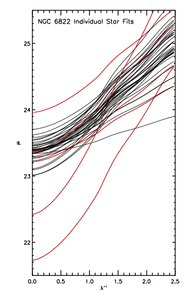
Figure 6.— Same as Figure 5, but without normalization applied and individual data points removed.. All 39 Cepheids are plotted, each with a smooth curve that follows the adopted reddening law. Cepheid fits excluded from the final distance calculation are plotted in red; these include the steep outliers and those discussed in the text. The lines of reddening intercept $\lambda^{-1}=0$ at the true modulus.

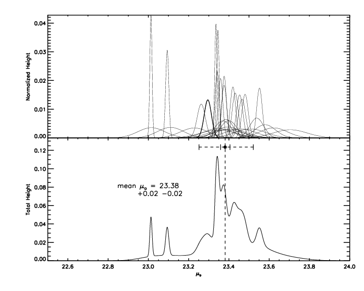
Figure 7.— Mixture distribution of distance moduli in Table 5. Top panel: Normal distributions with centers defined by $\mu_{o}$ and width ($\sigma$) corresponding to the error in $\mu_{o}$. Bottom: sum of the normal distributions in the top panel. The dashed vertical line corresponds to the mean, also plotted as a point above the distribution. The widest error bars correspond to the 1$\sigma$, or 34.1% of the total area starting from the center outward; the narrower error bars correspond to the the error in the mean divided by the square root of the number of stars used in the fit, i.e., $\sqrt{33}$.

Table 6True Distance Moduli from the Literature

Type	$\mu_{o}$	$\sigma_{stat}$	$\sigma_{sys}$	$\sigma_{tot}$	Reference
Cepheid ($VRIJHK_{s}[3.6]$)	23.38	0.02	0.03	—	This paper
Cepheid ($BVRI$)	23.49	0.08	—	—	Gallart et al. (1996)
Cepheid ($W_{V-I}$)	23.34	0.04	0.05	—	Pietrzyński et al. (2004)
Cepheid ($\bm{V}$)	23.29	0.05	—	—	Pietrzyński et al. (2004)
Cepheid ($\bm{I}$)	23.32	0.05	—	—	Pietrzyński et al. (2004)
Cepheid ($JK_{s}$)	23.31	0.02	0.06	—	Gieren et al. (2006)
Cepheid ($VIJHK_{s}$)	23.43	0.02	—	—	Feast et al. (2012)
RR-Lyrae	23.36	—	—	0.17	Clementini et al. (2003)
TRGB	23.46	—	—	0.10	Lee et al. (1993)
TRGB	23.20	0.05	0.2	—	Wyder (2003)
TRGB	23.53	0.05	—	—	Fusco et al. (2012)
Red Clump	23.34	0.10	0.2	—	Wyder (2003)
CMD (Field 1)	23.38	0.06	—	0.06	McQuinn et al. (2010)
CMD (Field 2)	23.39	—	—	0.06	McQuinn et al. (2010)
CMD (Field 3)	23.45	—	—	0.06	McQuinn et al. (2010)
CMD	23.40	—	—	—	Fusco et al. (2012)
Mira	23.56	0.03	—	—	Whitelock et al. (2013)

The errors given above correspond to the statistical, systematic or total error as defined by each reference.

5. Comparison with Previously Measured Distances

The distance moduli found using the two related methods agree well, which should be the case since they use similar datasets and assumptions about PL slopes. The new method based on individual stars, however, has the advantage of using the data more efficiently: it is not necessary to exclude any sub-samples lacking complete wavelength coverage.

Table 6 compiles distance moduli, reddenings, and their associated errors reported in the literature.

5.1. Cepheid Distance Comparison

The study with the largest sample of Cepheids by far is the work by Pietrzyński et al. (2004) as part of the Araucaria project. Their V & I observations combined with A${}_{V}=1.66$ mag and A_I=0.71 mag (using $E(B-V)=0.36$ mag from McAlary et al. 1983 and the reddening maps of Schlegel et al. 1998) yields extinction-corrected distance moduli $\mu_{oV}=23.29$ mag and $\mu_{oI}=23.32$ mag which they compare with their calculated Wesenheit W_VI value of $\mu_{W}=23.338$ mag. Interestingly, when we restrict our new method to only the V and I bands, we obtain a mean $E(B-V)=0.37$ mag and a modulus of $\mu_{o}=23.29$ mag which, accounting for the difference in $\mu_{LMC}$ used, agrees with Pietrzyński et al. (2004). When applying the the V & I-band PL relation slopes derived by the OGLE project (Udalski et al. 1999; Udalski 2000), we find the same distance modulus $\mu_{o}=23.38$, with a slightly higher mean $E(B-V)=0.38$.

The addition of multiple bands helps constrain the distance measured. BVRI photometry of 6 Cepheids by Gallart et al. (1996) yielded a higher value of $\mu=23.49\pm 0.08$ mag, though the reddening found in that work was a lower $E(B-V)$=0.24 mag. The addition of even a single near or mid-IR band helps to further constrain the extinction and correspondingly the measured distance modulus. The work by Gieren et al. (2006) as part of the Araucaria project combined J and K_s observations with the OGLE V and I data and found a total reddening of $E(B-V)$=0.356 mag and distance $\mu_{o}=23.312$ mag. When we restrict our new method to V, I, J and K_s only we find a higher $\mu_{o}=23.39$ mag, though this is likely due to the discrepancy between the J and K_s values used in our work: our adopted mean $\mu_{J}$ and $\mu_{K_{s}}$ are 0.14 and 0.10 mag fainter, respectively.

As our near-IR light curves are dominated by data from F12, the near-IR magnitudes we measure are consistent with those published in that study. With a few exceptions, our individual observations phase well within the light curves observed by F12. As such, the near-IR distances we derive are essentially equal to the apparent moduli in F12. They use a consistent set of Cepheids across all bands, and also re-fit the distance moduli in all bands using their own PL relations. Despite the agreement between our near-IR observations, the $\mu_{V}$ and $\mu_{I}$ F12 find are 0.32 and 0.14 mag lower than the values we derive, which leads to a correspondingly lower $E(B-V)=0.215$ mag in their work. This discrepancy is due to the difference in zero point and slope between their derived PL relation and the zero point and slopes we apply (Fouqué et al., 2007). This difference accounts for the higher $\mu_{VIJHK}=23.43$ mag in their work compared to our $\mu_{VIJHK}=23.36$.

5.2. TRGB Distance Comparison

In addition to the recent and substantial work on Cepheid distances, there are also a number of tip of the red giant branch (TRGB) distance measurements available for comparison to our work. The TRGB traces stars older than Cepheids and provides an independent measure of the distance. On average, TRGB measurements taken from the literature produce a larger distance than those measured with Cepheids, including our measurement.

The most recent study calculating a TRGB distance to NGC 6822 is Fusco et al. (2012). They perform a new photometric analysis of archival HST ACS observations, obtaining color-magnitude diagrams (CMD) for three fields. They determine a reddening using the similar CMD of the nearly extinction-free IC 1613, finding $E(B-V)=0.30\pm 0.032$ mag in their outer fields and $E(B-V)=0.37\pm 0.02$ mag in their inner field. The higher extinction in the central field calculated by Fusco et al. (2012) is consistent with the average reddening we calculate using our Cepheids, which have a distance from the center consistent with the location of their central field.

Fusco et al. (2012) use a new theoretical calibration to determine a TRGB distance of $\mu_{o}=23.54\pm 0.05$ mag, which is 0.16 mag larger than our distance, but consistent with the mean of other TRGB distance measurements. Although the values do not overlap within the statistical error, Fusco et al. (2012) note that their value is consistent with the Cepheid distance of F12 when the offset in the LMC distance is taken into account. This does not, however, account for the discrepancy between our value and that of Fusco et al. given the slightly larger difference in distance modulus and decreased uncertainty in $\mu_{LMC}$ (Freedman et al., 2011; Monson et al., 2012). The discrepancy may be due to metallicity. Fusco et al. note the tip of the red giant branch varies by 0.08 magnitudes over [Fe/H] from -0.8 to -2.0. Lee et al. (1993), for instance, find $\mu_{TRGB}=23.46\pm 0.1$ and [Fe/H]$=-1.8$; while Fusco et al. note in their discussion of metallicity effects that a value of $\mu_{o}=23.40$ would imply a much higher [Fe/H]$=-0.8$.

5.3. Other Methods

Some other distance measurements have been explored in the literature and can be compared with our Cepheid distance calculation. Clementini et al. (2003) examine a sample of short period variables in NGC 6822 and determine a distance using RR-Lyrae variables, which trace older field stars and provide an alternative pathway to distance calibration. They find a distance of $\mu_{o}=23.36\pm 0.17$, which, given the error, is consistent with both our estimate and the TRGB distance given in Fusco et al. (2012).

McQuinn et al. (2010) use HST WFPC2 data and a CMD fitting routine to determine distance moduli of $\mu_{o}=23.38,23.39$ and $23.445$ mag in three different fields. They also fit a corresponding A${}_{V}=1.1,1.1$ and $0.7$ mag, consistent with our results. Wyder (2003) also examines HST WFPC2 data and derive a CMD in several fields, and find a distance using the red clump of $\mu_{o}=23.34\pm 0.1$ mag. The TRGB distance derived by Wyder is much lower, at $\mu_{o}=23.20\pm 0.05(random)\pm 0.2(systematic)$ mag, which the author attributes to a large systematic uncertainty due to chemical enrichment. This is in contrast with Fusco et al. (2012), whose $\mu_{cmd}=23.40$ is 0.14 mag less than their $\mu_{TRGB}$.

Finally, Whitelock et al. (2013) use Mira variables to derive a distance of $\mu_{o}=23.56\pm 0.03$ mag. Even accounting for the 0.03 mag difference in the $\mu_{LMC}$ used (18.50 vs. our 18.47) this value deviates significantly from our measurement. Whitelock et al. (2013) adopt a lower extinction value of A${}_{V}=0.77$ mag from Clementini et al. (2003) and extinction values from Schlegel et al. (1998). Even with their near-IR observations, when compared with our adopted extinction this can lead to a difference of 0.09 magnitudes at J and 0.05 magnitudes at K which begins to account for the difference.

6. Conclusions

In this study we presented a new distance measurement to the nearby dwarf starburst NGC 6822 derived using multiple passband observations. In addition to previously published data we utilized new, previously unpublished mid-infrared Spitzer data and new near-IR FourStar observations. Using both old and new multi-epoch data, we calculated new mean magnitudes for 39 cepheids in the V, I, J, H, K_s, 3.6 $\mu$m and 4.5 $\mu$m bands.

In addition to calculating distance moduli for each band and calculating an average line-of-sight extinction and true distance, we introduce a new method for dealing with different samples of available Cepheids at different wavelengths. We use the mean magnitudes for each individual star to fit a distance modulus $\mu$ to that star and corresponding extinction. We then use the resulting individual moduli to create a mixture distribution from which we derive a true, extinction-corrected distance modulus of $\mu_{o}=23.38\pm 0.02$ mag.

We compare our results with both previous distance measurements using Cepheid variables as well as other distance measures. Our value agrees broadly with other distances calculated in the literature, though our result shows a discrepancy compared to the newest calculation of a TRGB distance to NGC 6822 by Fusco et al. (2012).

This appendix contains supplemental information about the objects and analysis used in this paper. Table A1 lists the coordinates of the cepheids used in this paper, adopted from Pietrzyński et al. (2004), adjusted slightly to account for an apparent offset of approximately 1.4″west and 0.8″north. Figure A.2 shows postage-stamp images of Cepheids with FourStar data used in our analysis. Figs. A.2 through A.11 show the light curves fit to the individual passbands using GLOESS, as shown first in Figure 2.

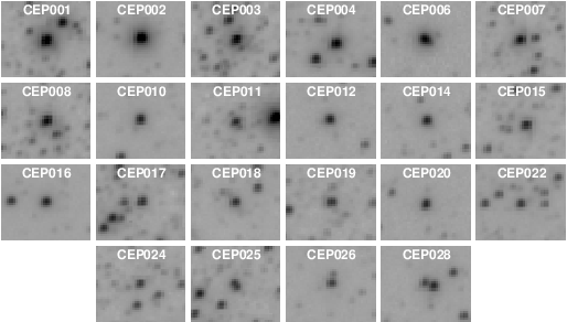
Figure A.1.— Postage stamps of the Cepheids with near-IR magnitudes measured in our analysis. The images are from our May 7, 2012 FourStar observations for which we had exceptionally good seeing.

Table A.1Cepheid Coordinates

Designation	$RA(J2000)$	$Dec(J2000)$	Designation	$RA(J2000)$	$Dec(J2000)$
CEP001	19:45:01.92	-14:47:32.3	CEP021	19:45:46.53	-14:56:41.6
CEP002	19:44:56.72	-14:53:14.9	CEP022	19:44:50.06	-14:52:28.2
CEP003	19:44:55.13	-14:47:11.9	CEP023	19:45:04.46	-14:55:07.7
CEP004	19:44:56.66	-14:51:17.7	CEP024	19:44:50.84	-14:48:36.5
CEP005	19:45:24.95	-14:58:44.0	CEP025	19:45:00.37	-14:47:04.0
CEP006	19:45:15.71	-14:55:23.4	CEP026	19:45:04.37	-14:52:52.7
CEP007	19:44:59.62	-14:47:10.0	CEP027	19:45:04.55	-14:53:39.8
CEP008	19:44:52.95	-14:46:55.8	CEP028	19:45:05.57	-14:53:20.1
CEP009	19:45:43.20	-14:45:42.3	CEP029	19:45:02.84	-14:51:56.5
CEP010	19:45:02.13	-14:53:43.4	CEP030	19:44:51.90	-14:45:51.4
CEP011	19:44:52.32	-14:47:35.6	CEP031	19:44:51.02	-14:47:19.8
CEP012	19:45:08.17	-14:53:49.1	CEP032	19:45:27.76	-14:53:51.6
CEP013	19:44:47.08	-14:49:21.1	CEP033	19:45:01.53	-14:49:21.1
CEP014	19:45:06.35	-14:51:04.0	CEP034	19:45:08.67	-14:49:09.9
CEP015	19:44:56.46	-14:50:33.5	CEP035	19:45:01.49	-14:43:09.3
CEP016	19:44:51.22	-14:54:18.3	CEP036	19:45:19.40	-14:45:57.6
CEP017	19:44:52.99	-14:48:39.0	CEP037	19:44:50.96	-14:46:05.2
CEP018	19:45:02.45	-14:51:06.0	CEP038	19:44:30.61	-14:51:21.3
CEP019	19:44:50.25	-14:49:12.8	CEP039	19:45:23.78	-14:46:32.5
CEP020	19:45:23.38	-14:46:18.2	…	…	…

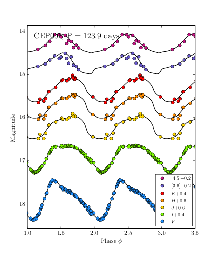
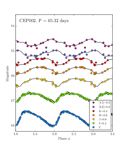
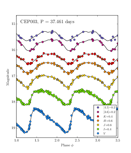
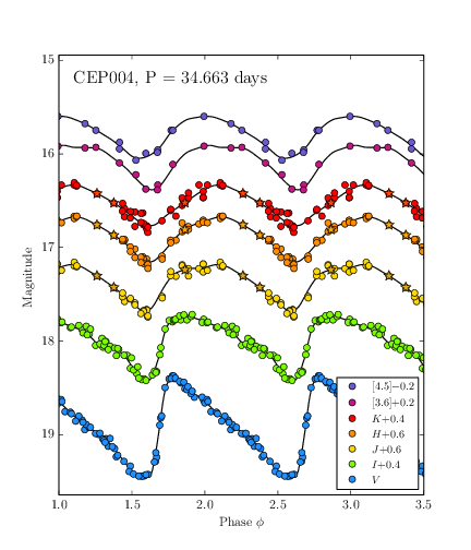
Figure A.2.— Light curves for the GLOESS fits to four Cepheids (CEP001, CEP002, CEP003, CEP004), as in Fig. 2. The average magnitude and its error are calculated using the GLOESS fits, shown in this plot as the continuous lines. In cases where the data were not well-sampled, J, H or K_s magnitudes are not plotted and were calculated by finding the average value of the data points (see Table 2). The FourStar data, plotted as stars, agree with those of F12, as discussed in section 2.4. The J, H and K_s fits are dominated by the F12 data.

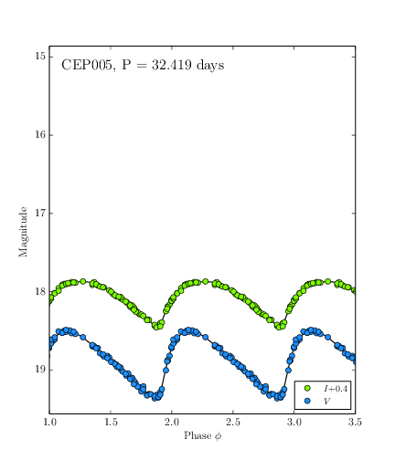
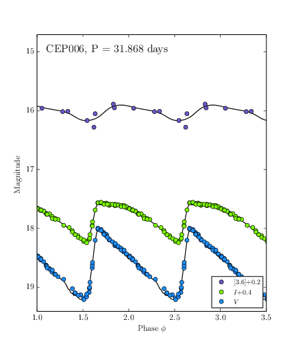
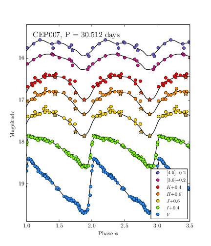
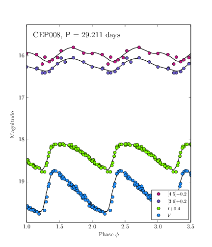
Figure A.3.— Same as Figure A2, but for CEP005, CEP006, CEP007 and CEP008.

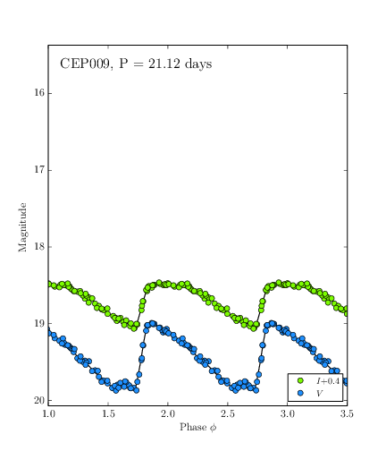
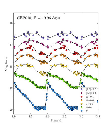
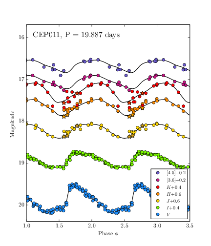
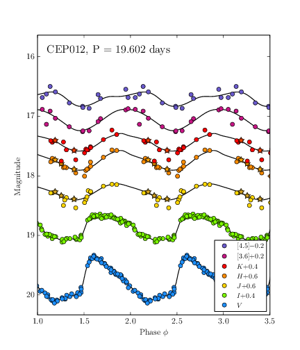
Figure A.4.— Same as Figure A2, but for CEP009, CEP010, CEP011 and CEP012.

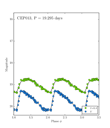
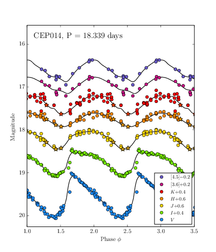
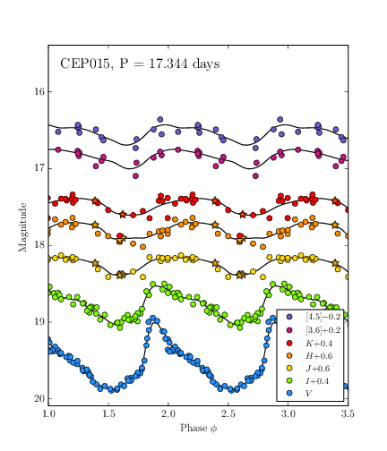
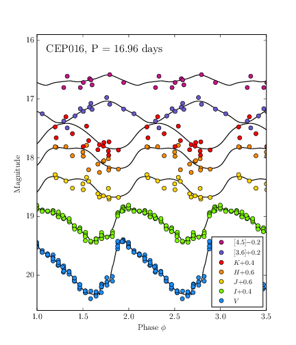
Figure A.5.— Same as Figure A2, but for CEP013, CEP014, CEP015 and CEP016.

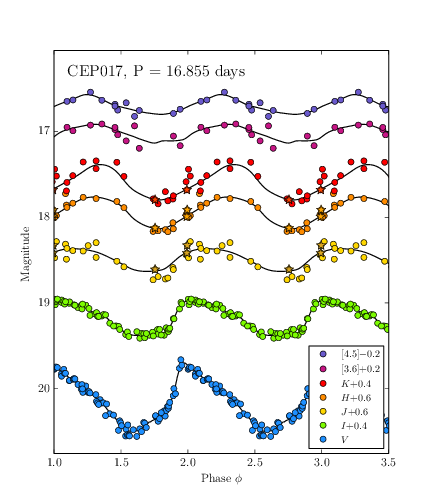
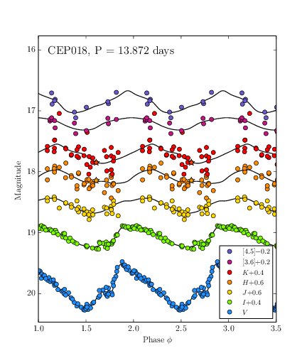
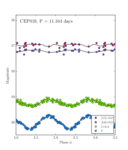
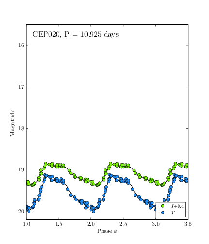
Figure A.6.— Same as Figure A2, but for CEP017, CEP018, CEP019 and CEP020.

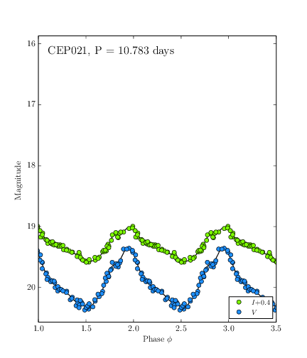
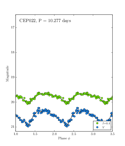
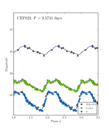
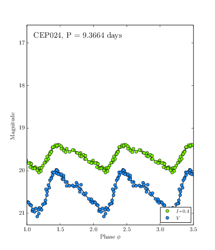
Figure A.7.— Same as Figure A2, but for CEP021, CEP022, CEP023 and CEP024.

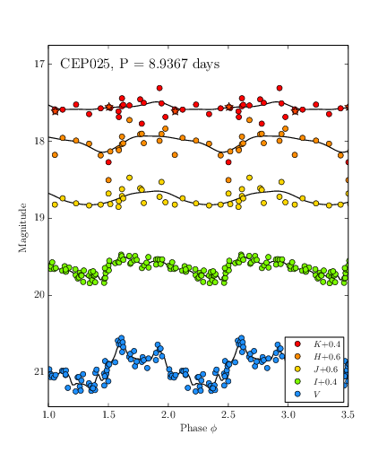
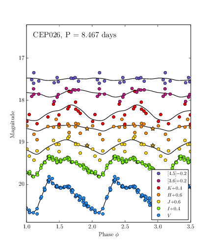
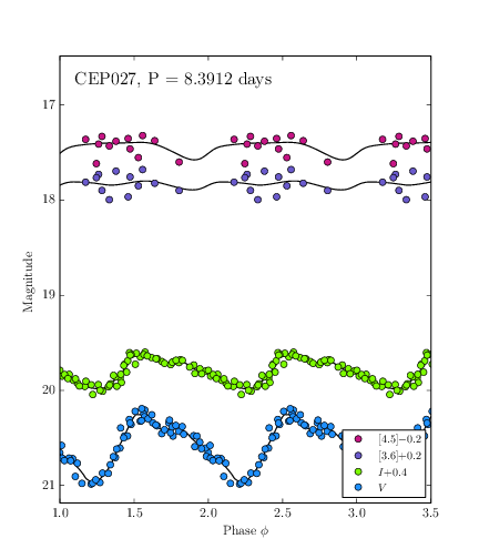
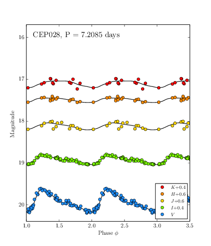
Figure A.8.— Same as Figure A2, but for CEP025, CEP026, CEP027 and CEP028.

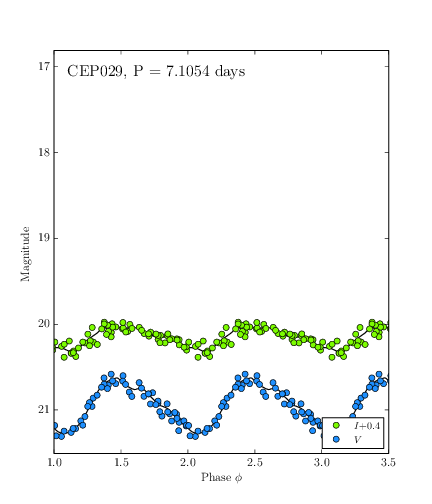
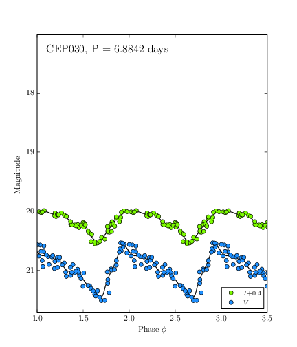
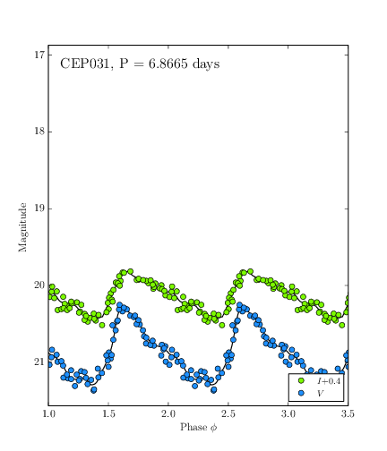
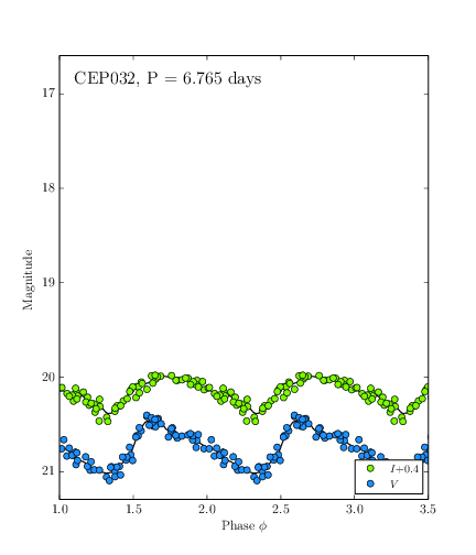
Figure A.9.— Same as Figure A2, but for CEP029, CEP030, CEP031 and CEP032.

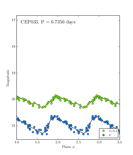
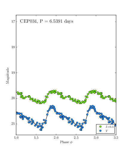
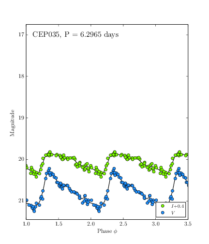
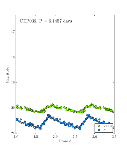
Figure A.10.— Same as Figure A2, but for CEP033, CEP034, CEP035 and CEP036.

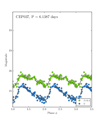
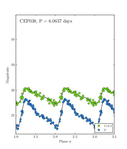
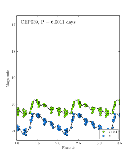
Figure A.11.— Same as Figure A2, but for CEP037, CEP038 and CEP039.

References

- Antonello et al. (2002) Antonello, E., Fugazza, D., Mantegazza, L., Stefanon, M., & Covino, S. 2002, A&A, 386, 860
- Cardelli et al. (1989) Cardelli, J. A., Clayton, G. C., & Mathis, J. S. 1989, ApJ, 345, 245
- Carpenter (2001) Carpenter, J. M. 2001, AJ, 121, 2851
- Clementini et al. (2003) Clementini, G., Held, E. V., Baldacci, L., & Rizzi, L. 2003, ApJ, 588, L85
- Feast et al. (2012) Feast, M. W., Whitelock, P. A., Menzies, J. W., & Matsunaga, N. 2012, MNRAS, 421, 2998
- Fouqué et al. (2007) Fouqué, P., et al. 2007, A&A, 476, 73
- Freedman (1985) Freedman, W. L. 1985, in IAU Colloq. 82: Cepheids: Theory and Observation, ed. B. F. Madore, 225
- Freedman (1988) Freedman, W. L. 1988, ApJ, 326, 691
- Freedman et al. (1985) Freedman, W. L., Grieve, G. R., & Madore, B. F. 1985, ApJS, 59, 311
- Freedman et al. (2012) Freedman, W. L., Madore, B. F., Scowcroft, V., Burns, C., Monson, A., Persson, S. E., Seibert, M., & Rigby, J. 2012, ApJ, 758, 24
- Freedman et al. (1991) Freedman, W. L., Wilson, C. D., & Madore, B. F. 1991, ApJ, 372, 455
- Freedman et al. (2011) Freedman, W. L., et al. 2011, AJ, 142, 192
- Fusco et al. (2012) Fusco, F., Buonanno, R., Bono, G., Cassisi, S., Monelli, M., & Pietrinferni, A. 2012, A&A, 548, A129
- Gallart et al. (1996) Gallart, C., Aparicio, A., & Vilchez, J. M. 1996, AJ, 112, 1928
- Gieren et al. (2006) Gieren, W., Pietrzyński, G., Nalewajko, K., Soszyński, I., Bresolin, F., Kudritzki, R.-P., Minniti, D., & Romanowsky, A. 2006, ApJ, 647, 1056
- Hubble (1925) Hubble, E. P. 1925, ApJ, 62, 409
- Joye & Mandel (2003) Joye, W. A., & Mandel, E. 2003, in Astronomical Society of the Pacific Conference Series, Vol. 295, Astronomical Data Analysis Software and Systems XII, ed. H. E. Payne, R. I. Jedrzejewski, & R. N. Hook, 489–+
- Kayser (1967) Kayser, S. E. 1967, AJ, 72, 134
- Kennicutt et al. (2003) Kennicutt, Jr., R. C., et al. 2003, PASP, 115, 928
- Lee et al. (1993) Lee, M. G., Freedman, W. L., & Madore, B. F. 1993, ApJ, 417, 553
- Madore (1976) Madore, B. F. 1976, in Royal Greenwich Observatory Bulletins, Vol. 182, The Galaxy and the Local Group, ed. R. J. Dickens, J. E. Perry, F. G. Smith, & I. R. King, 153
- Madore (1982) Madore, B. F. 1982, ApJ, 253, 575
- Madore et al. (2009) Madore, B. F., Rigby, J., Freedman, W. L., Persson, S. E., Sturch, L., & Mager, V. 2009, ApJ, 693, 936
- McAlary et al. (1983) McAlary, C. W., Madore, B. F., McGonegal, R., McLaren, R. A., & Welch, D. L. 1983, ApJ, 273, 539
- McQuinn et al. (2010) McQuinn, K. B. W., et al. 2010, ApJ, 721, 297
- Monson et al. (2012) Monson, A. J., Freedman, W. L., Madore, B. F., Persson, S. E., Scowcroft, V., Seibert, M., & Rigby, J. R. 2012, ApJ, 759, 146
- Persson et al. (2004) Persson, S. E., Madore, B. F., Krzemiński, W., Freedman, W. L., Roth, M., & Murphy, D. C. 2004, AJ, 128, 2239
- Persson et al. (2013) Persson, S. E., et al. 2013, PASP, 125, 654
- Pietrzyński et al. (2004) Pietrzyński, G., Gieren, W., Udalski, A., Bresolin, F., Kudritzki, R.-P., Soszyński, I., Szymański, M., & Kubiak, M. 2004, AJ, 128, 2815
- Pietrzyński et al. (2013) Pietrzyński, G., et al. 2013, Nature, 495, 76
- Reach et al. (2005) Reach, W. T., et al. 2005, PASP, 117, 978
- Schlegel et al. (1998) Schlegel, D. J., Finkbeiner, D. P., & Davis, M. 1998, ApJ, 500, 525
- Scowcroft et al. (2013) Scowcroft, V., Freedman, W. L., Madore, B. F., Monson, A. J., Persson, S. E., Seibert, M., Rigby, J. R., & Melbourne, J. 2013, ApJ, 773, 106
- Scowcroft et al. (2011) Scowcroft, V., Freedman, W. L., Madore, B. F., Monson, A. J., Persson, S. E., Seibert, M., Rigby, J. R., & Sturch, L. 2011, ApJ, 743, 76
- Soszyński et al. (2005) Soszyński, I., Gieren, W., & Pietrzyński, G. 2005, PASP, 117, 823
- Stetson (1987) Stetson, P. B. 1987, PASP, 99, 191
- Stetson (1994) —. 1994, PASP, 106, 250
- Udalski (2000) Udalski, A. 2000, Acta Astron., 50, 279
- Udalski et al. (1999) Udalski, A., Szymanski, M., Kubiak, M., Pietrzynski, G., Soszynski, I., Wozniak, P., & Zebrun, K. 1999, Acta Astron., 49, 201
- Walker (2012) Walker, A. R. 2012, Ap&SS, 341, 43
- Whitelock et al. (2013) Whitelock, P. A., Menzies, J. W., Feast, M. W., Nsengiyumva, F., & Matsunaga, N. 2013, MNRAS, 428, 2216
- Wyder (2003) Wyder, T. K. 2003, AJ, 125, 3097