All graphs have tree-decompositions displaying their topological ends

Abstract

We show that every connected graph has a spanning tree that displays all its topological ends. This proves a 1964 conjecture of Halin in corrected form, and settles a problem of Diestel from 1992.

1 Introduction

In 1931, Freudenthal introduced a notion of ends for second countable Hausdorff spaces [20], and in particular for locally finite graphs [21]. Independently, in 1964, Halin [23] introduced a notion of ends for graphs, taking his cue directly from Carathéodory’s Primenden of simply connected regions of the complex plane [4]. For locally finite graphs these two notions of ends agree.

For graphs that are not locally finite, Freudenthal’s topological definition still makes sense, and gave rise to the notion of topological ends of arbitrary graphs [17]. In general, this no longer agrees with Halin’s notion of ends, although it does for trees.

Halin [23] conjectured that the end structure of every connected graph can be displayed by the ends of a suitable spanning tree of that graph. He proved this for countable graphs. Halin’s conjecture was finally disproved in the 1990s by Seymour and Thomas [27], and independently by Thomassen [30].

In this paper we shall prove Halin’s conjecture in amended form, based on the topological notion of ends rather than Halin’s own graph-theoretical notion. We shall obtain it as a corollary of the following theorem, which proves a conjecture of Diestel [13] of 1992 (again, in amended form):

Theorem 1.

Every graph has a tree-decomposition $(T,{{\cal V}})$ of finite adhesion such that the ends of $T$ define precisely the topological ends of $G$.
See Section 2 for definitions.

The tree-decompositions constructed for the proof of Theorem 1 have several further applications. In [6] we use them to answer the question to what extent the ends of a graph - now in Halin’s sense - have a tree-like structure at all. In [8], we apply Theorem 1 to show that the topological cycles of any graph together with its topological ends induce a matroid. We remark that although the existence of a tree-decomposition as in Theorem 1 for an arbitrarily subset of the vertex-ends in place of the topological ends implies the existence of a suitable spanning tree in Halin’s sense for that subset by Section 6, the converse is not true, see Section 3.

This paper is organised as follows. In Section 2 we explain the problems of Diestel and Halin in detail, after having given some basic definitions. In Section 3 we continue with examples related to these problems. Section 4 only contains material that is relevant for Section 5 in which we prove that every graph has a nested set of separations distinguishing the vertex-ends efficiently. In Section 6, we use this theorem to prove Theorem 1. Then we deduce Halin’s amended conjecture. Finally, Section 7 contains concluding remarks.

2 Definitions

Throughout, notation and terminology for graphs are that of [14]. And $G$ always denotes a graph.

A vertex-end in a graph $G$ is an equivalence class of rays (one-way infinite paths), where two rays are equivalent if they cannot be separated in $G$ by removing finitely many vertices. Put another way, this equivalence relation is the transitive closure of the relation relating two rays if they intersect infinitely often.

Example .

The vertex-ends of rooted trees are (in bijection with) the rays starting at the root; of course vertex-ends do not depend on the choice of a root.

Let $X$ be a locally connected Hausdorff space. Given a subset $Y\subseteq X$, we write $\overline{Y}$ for the closure of $Y$, and $F(Y):=\overline{Y}\cap\overline{X\setminus Y}$ for its frontier. In order to define the topological ends of $X$, we consider infinite sequences ${U_{1}\supseteq U_{2}\supseteq...}$ of non-empty connected open subsets of $X$ such that each $F(U_{i})$ is compact and $\bigcap_{i\geq 1}\overline{U}_{i}=\emptyset$. We say that two such sequences ${U_{1}\supseteq U_{2}\supseteq...}$ and ${U_{1}^{\prime}\supseteq U_{2}^{\prime}\supseteq...}$ are equivalent if for every $i$ there is some $j$ with $U_{i}\supseteq U_{j}^{\prime}$. This relation is transitive and symmetric [20, Satz 2]. The equivalence classes of those sequences are the topological ends of $X$ [17, 20, 26].

For the simplicial complex of a graph $G$, Diestel and Kühn described the topological ends combinatorically: a vertex dominates a vertex-end $\omega$ if for some (equivalently: every) ray $R$ belonging to $\omega$ there is an infinite fan of $v$-$R$-paths that are vertex-disjoint except at $v$. In [17], they proved that the topological ends are given by the undominated vertex-ends. Hence in this paper, we take this as our definition of topological end of $G$.

Example .

For locally finite graphs the notions of vertex-ends and topological ends agree.

Example .

For trees the notions of vertex-ends and topological ends agree. Hence we just call the vertex-ends of trees ends.

For us, a separation is an (ordered) pair $(A,B)$ of vertex sets $A$ and $B$ such that no edge has an endvertex in $A\setminus B$ and the other endvertex in $B\setminus A$. The set $A\cap B$ is called the separator of $(A,B)$. The size of the separator is the order of $(A,B)$. The sets $A$ and $B$ are called the sides of the separation. The reverse of the separation $(A,B)$ is the separation $(B,A)$.

Given two separations $(A,B)$ and $(C,D)$, we write $(A,B)\leq(C,D)$ if $A\subseteq C$ and $D\subseteq B$. These separations are nested if $(A,B)\leq(C,D)$ or one of the other three possibilities obtained by replacing $(A,B)$ or $(C,D)$ by their reverse. Formally, $(A,B)$ and $(C,D)$ are nested if $(A,B)\leq(C,D)$, $(B,A)\leq(C,D)$, $(A,B)\leq(D,C)$ or $(B,A)\leq(D,C)$.

Remark .

Most separations of interest are ‘proper’, see below. By Section 2, proper separations $(A,B)$ and $(C,D)$ satisfy $(A,B)\leq(C,D)$ already if $A\subseteq C$. In this sense our definition of nestedness corresponds to the notion of nestedness for sets.

A separation $(A,B)$ is proper if every vertex in the separator $A\cap B$ has a neighbour in $A\setminus B$ and $B\setminus A$.

Observation .

For proper separations $(A,B)$ and $(C,D)$ the following are equivalent.

1. $(A,B)\leq(C,D)$;

2. $A\subseteq C$;

3. $A\setminus B\subseteq C\setminus D$.

Proof.

As $(A,B)$ is proper, the side $A$ is determined by the set $A\setminus B$; indeed, it is $A\setminus B$ together with its neighbourhood. Conversely, also the side $A$ determines the set $A\setminus B$: this set consists of those vertices of $A$ that have all their neighbours in $A$. So (2) and (3) are equivalent.

Clearly (1) implies (2). Now conversely assume that $A\subseteq C$. By the above it suffices to show that $D\setminus C$ is included in $B\setminus A$. In other words: $G\setminus C$ is included in $G\setminus A$. This follows from $A\subseteq C$. ∎

A vertex-end $\omega$ lives in a side $B$ of a separation $(A,B)$ of finite order if the side $B$ includes a ray belonging to $\omega$. In this case $B$ includes a subray of every ray belonging to $\omega$, see Figure 1.

Figure 1: Every ray traverses the finite separator $A\cap B$ finitely often and then is eventually included in one of the sides $A$ or $B$.

A separation $(A,B)$ of finite order distinguishes two vertex-ends $\omega$ and $\mu$ if one of them lives in the side $A$ and the other lives in the side $B$. It distinguishes them efficiently if $(A,B)$ has minimal order amongst all separations distinguishing $\omega$ and $\mu$.

A tree-decomposition of a graph $G$ consists of a tree $T$ together with a family of subgraphs $(P_{t}|t\in V(T))$ of $G$ such that every vertex and edge of $G$ is in at least one of these subgraphs, and such that if $v$ is a vertex of both $P_{t}$ and $P_{w}$, then it is a vertex of each $P_{u}$, where $u$ lies on the $v$-$w$-path in $T$. We call the subgraphs $P_{t}$ the parts of the tree-decomposition. The adhesion of a tree-decomposition is finite if adjacent parts intersect only finitely. Given an edge $tu$ of $T$, we denote by $T_{t}$ the subtree of $T-tu$ that contains $t$. Given a directed edge $tu$ of $T$, the separation corresponding to $tu$ is the separation $(A_{t},A_{u})$, where $A_{i}$ is the union of all parts $P_{x}$ with $x\in T_{i}$ for $i=u,t$.

In [2, 25, 29], tree-decompositions of finite adhesion are used to study the structure of infinite graphs. In [13, Problem 4.3], Diestel wanted to know whether every graph $G$ has a tree-decomposition $(T,P_{t}|t\in V(T))$ of finite adhesion that somehow encodes the structure of the graph with its ends.

Let us be more precise. Given a vertex-end $\omega$, we take $O(\omega)$ to consist of those oriented edges $tu$ of $T$ such that $\omega$ lives in its corresponding separation. Note that $O(\omega)$ contains precisely one of the two directions $tu$ and $ut$ of each edge of the tree. Furthermore this orientation $O(\omega)$ of $T$ points towards a node of $T$ or to an end of $T$. We say that $\omega$ lives in the part for that node or that end, respectively.

A vertex-end $\omega$ is thin if every set of vertex-disjoint rays belonging to $\omega$ is finite; otherwise $\omega$ is thick. Diestel asked whether every graph has a tree-decomposition $(T,P_{t}|t\in V(T))$ of finite adhesion such that different thick vertex-ends live in different parts and such that the ends of $T$ define precisely the thin vertex-ends; here the ends of $T$ define precisely a set $\Psi$ of vertex-ends of $G$ if in every end of $T$ there lives a unique vertex-end and it is in $\Psi$ and conversely every vertex-end in $\Psi$ lives in some end of $T$, see Figure 2.

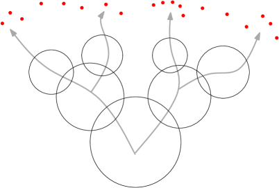
Figure 2: The ends of the decomposition tree - this tree is indicated in grey - define precisely the vertex-ends of the graph indicated by dots. Other vertex-ends living in parts are not drawn.

Unfortunately, that is not true; in Section 3, we construct a graph such that each of its tree-decompositions of finite adhesion has a part in which two (thick) vertex-ends live. In Section 3 we refine that construction by constructing a graph such that there live two thin vertex-ends in some part of every such a tree-decomposition.

Hence there remains the open question whether there is a natural subclass of the vertex-ends (similar to the class of thin vertex-ends) such that every graph has a tree-decomposition of finite adhesion such that the ends of its decomposition tree define precisely the vertex-ends in that subclass. Another question that arises in this context is: what is the largest possible natural class of vertex-ends such that every graph has a tree-decomposition distinguishing the vertex-ends in that class? Theorem 1 above answers the first question affirmatively. In Section 7, we show how Theorem 1 can be used to obtain a satisfying answer to the second question.

It is impossible to construct a tree-decomposition as in Theorem 1 with the additional property that for any two topological ends $\omega$ and $\mu$, there is a separation corresponding to an edge of the tree that separates $\omega$ and $\mu$ efficiently, see Section 3.

A recent development in the theory of infinite graphs seeks to extend theorems about finite graphs and their cycles to infinite graphs and the topological circles formed with their ends, see for example [1, 3, 18, 19, 22, 28], and [12] for a survey. We expect that Theorem 1 has further applications in this direction aside from the one mentioned in the introduction.

A rooted spanning tree $T$ of a graph $G$ is end-faithful for a set $\Psi$ of vertex-ends if each vertex-end $\omega\in\Psi$ is uniquely represented by $T$ in the sense that $T$ contains a unique ray belonging to $\omega$ and starting at the root. For example, every normal spanning tree is end-faithful for all vertex-ends. Halin conjectured that every connected graph has an end-faithful tree for all vertex-ends. At the end of Section 6, we show that Theorem 1 implies the following nontrivial weakening of this disproved conjecture:

Corollary .

Every connected graph has an end-faithful spanning tree for the topological ends.

One might ask whether it is possible to construct an end-faithful spanning tree for the topological ends with the additional property that it does not include any ray to any other vertex-end. However, this is not possible in general. Indeed, Seymour and Thomas constructed a graph $G$ with no topological end that does not have a rayless spanning tree [27].

3 Example section

Example .

In this example we give two constructions of graphs that have no tree-decompositions of finite adhesion that distinguish all vertex-ends. These constructions motivate the construction of Section 3, where we can construct such a graph not only for the class of vertex-ends but for the finer class of thin vertex-ends.

The simplest example of a graph with no such tree-decomposition for the vertex-ends known to the author is the (infinite) binary tree with tops, see Figure 3; this graph is obtained from the binary tree $T_{2}$ by adding one new vertex for every ray starting at the root. This new vertex is adjacent to all vertices on that ray. We call these new vertices the tops.

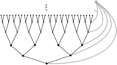
Figure 3: The binary tree is indicated in black. In grey we indicated the addition of a top along the right most ray.

We omit the proof that this graph has no tree-decompositions of finite adhesion that distinguishes all vertex-ends.

A slightly more complicated example is obtained from the regular tree $T_{\omega}$ with countably infinite degree by adding fat tops; here adding fat tops means that at each ray of $T_{\omega}$ starting at the root, we attach uncountably many, say $\aleph_{1}$, tops (that is new vertices adjacent to all vertices on the ray).

We sketch the proof that $T_{\omega}$ with fat tops has no tree-decompositions of finite adhesion that distinguishes all vertex-ends. First one checks that the vertex-ends of $T_{\omega}$ with fat tops are the ends of $T_{\omega}$ (this proof is similar to Section 3 below). The vertex-ends of $T_{\omega}$ with fat tops, however, are fat, that is, they are dominated by uncountably many vertices. The key observation is the following.

Lemma .

Let $H$ be any graph with a tree-decomposition $(T,{{\cal V}})$ of finite adhesion. Then no fat vertex-end of $H$ lives in an end of $T$.

Proof.

Vertex-ends living in ends $\mu$ of $T$ can only be dominated by those vertices that eventually are in the separators corresponding to the edges on some ray in $\mu$. Since the tree-decomposition has finite adhesion, there can only be countably many such vertices. So vertex-ends living in ends of the decomposition tree cannot be fat. ∎

In the final step one assumes that some tree-decomposition of finite adhesion distinguishes all vertex-ends. Since the graph $T_{\omega}$ is countable, it can only have countably many separators. A finite separator of $T_{\omega}$ with fat tops separates the same vertex-ends as their restriction to $T_{\omega}$ does. This essentially means that the decomposition tree has only countably many edges. So it can only have countably many nodes. Since there are uncountably many vertex-ends, two of them have to live in the same part as they cannot live in an end of the decomposition tree by Section 3.

We remark that this proof also works for any graph obtained from $T_{\omega}$ by attaching some $\aleph_{1}$ fat tops at $T_{\omega}$. So there is a counterexample against the statement that every graph has a tree-decomposition of finite adhesion distinguishing its vertex-ends of cardinality $\aleph_{1}$ – which is independent of the Continuum Hypothesis.

Example .

In this example we construct a graph $G$ such that each of its tree-decomposition of finite adhesion cannot distinguish all thin vertex-ends.

We start the construction with the regular tree $T_{\omega}$ of countably infinite degree. For each vertex of $T_{\omega}$, we add a ray through its neighbours in the next level. Call the resulting graph $G^{\prime}$, see Figure 4.

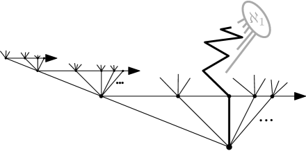
Figure 4: The graph $G^{\prime}$ is indicated in black. We indicated in grey the addition of fat tops at the highlighted ray. We obtain the graph $G$ from the graph $G^{\prime}$ by adding these fat tops at all rays starting at the root.

The vertex-ends of $G^{\prime}$ are those of $T_{\omega}$ together with one vertex-end for every newly added ray.

We obtain $G$ from $G^{\prime}$ by adding for every ray of $T_{\omega}$ starting at the root a clique of uncountable cardinality $\aleph_{1}$ that is complete to that ray.

Lemma .

The vertex-ends of $G^{\prime}$ are (in bijection with) the vertex-ends of $G$.

Proof.

Every ray of $G$ is equivalent to a ray of $G^{\prime}$. Conversely any two vertex-ends of $G^{\prime}$ can be separated by a path of $T_{\omega}$ starting at the root. This path still separates rays belonging to these vertex-ends of $G^{\prime}$ in $G$. Hence $G$ and $G^{\prime}$ have the same vertex-ends.

∎

The thin vertex-ends of $G$ are those vertex-ends of $G^{\prime}$ coming from newly added rays; indeed, if we remove the finite path of $T_{\omega}$ below such a newly added ray, all vertices on that ray become cut-vertices. All other vertex-ends are each dominated by uncountably many vertices, that is, they are fat.

We use the vertices of $T_{\omega}$ to refer to the thin vertex-ends. More precisely, we say that the vertex-end sitting above a vertex $v$ is the one to which the ray in the upward neighbourhood of $v$ belongs.

Suppose for a contradiction that the graph $G$ has a tree-decomposition $(T,P_{t}|t\in V(T))$ of finite adhesion that distinguishes all its thin vertex-ends. First we show the following.

Lemma .

There is a ray $R$ of $T$ such that a fat vertex-end of $G$ lives in the end to which $R$ belongs.

Proof.

Our aim is to construct a sequence $(v_{n}|n\in{\mathbb{N}})$ of vertices that lie on a ray of the tree $T_{\omega}$ starting at the root together with a sequence $((A_{n},B_{n})|n\in{\mathbb{N}}^{*})$ of separations corresponding to edges of the decomposition tree such that $(A_{n},B_{n})\leq(A_{n+1},B_{n+1})$ and $v_{n}$ is contained in $B_{n}\setminus A_{n}$.

We start the construction by picking an arbitrary separation $(C,D)$ corresponding to an edge of the decomposition tree such that it distinguishes two thin vertex-ends. We pick for $v_{0}$ the root of the tree $T_{\omega}$. By replacing the separation $(C,D)$ by its reverse $(D,C)$ if necessary, we may assume that the thin vertex-end sitting above $v_{0}$ lives in the side $C$. We let $(A_{1},B_{1})=(C,D)$. Let $\mu$ be a thin vertex-end living in $B_{1}$ and let $u$ be the vertex of $T_{\omega}$ above which $\mu$ sits. The vertex $u$ must be contained in the side $B_{1}$ and have all but finitely many of its upward-neighbours in the side $B_{1}$. Since the separator $A_{1}\cap B_{1}$ is finite, the vertex $u$ has an upward-neighbour $v_{1}$ in the rooted tree $T_{\omega}$ that is contained in $B_{1}\setminus A_{1}$. We let $P_{1}$ be the unique path included in the tree $T_{\omega}$ from the vertex $v_{0}$ to the vertex $v_{1}$.

Now assume that we already constructed a path $P_{n}$ and a separation $(A_{n},B_{n})$ corresponding to an edge of the decomposition tree such that the last vertex $v_{n}$ of $P_{n}$ is contained in $B_{n}\setminus A_{n}$ and is a vertex of $T_{\omega}$. Next we construct the path $P_{n+1}$ and the separation $(A_{n+1},B_{n+1})$. As the separator $A_{n}\cap B_{n}$ is finite, the vertex $v_{n}$ has two upward-neighbours $u$ and $u^{\prime}$ in the rooted tree $T_{\omega}$ contained in $B_{n}\setminus A_{n}$. By assumption there is a separation $(C,D)$ corresponding to an edge of the decomposition tree such that the thin vertex-ends sitting above $u$ and $u^{\prime}$ are distinguished by $(C,D)$.

Sublemma .

The separation $(A_{n},B_{n})$ is $\leq$ to the separation $(C,D)$ or its reverse $(D,C)$.

Proof.

This is a simple consequence of the fact that the separations $(C,D)$ and $(A_{n},B_{n})$ are nested as separations corresponding to edges of a decomposition tree of the same tree-decomposition.

The sides $C$ and $B_{n}$ both contain all but finitely many vertices of every ray belonging to the vertex-end sitting above the vertex $u$. Hence the intersection $C\cap B_{n}$ is infinite. Similarly, we conclude that the intersection $D\cap B_{n}$ is infinite. As the separator $C\cap D$ is finite, the side $B_{n}$ cannot be included in one of the sides $C$ or $D$. Hence as the separations $(C,D)$ and $(A_{n},B_{n})$ are nested, it must be that the separation $(A_{n},B_{n})$ is $\leq$ to the separation $(C,D)$ or its reverse $(D,C)$. ∎

By replacing the separation $(C,D)$ by its reverse $(D,C)$ if necessary we may assume by Section 3 that $(A_{n},B_{n})\leq(C,D)$. We let $(A_{n+1},B_{n+1})=(C,D)$. Since the separator $A_{n+1}\cap B_{n+1}$ is finite and the thin vertex-end sitting above $u^{\prime}$ lives in $B_{n+1}$, the vertex $u^{\prime}$ has an upward-neighbour $v_{n+1}$ in the rooted tree $T_{\omega}$ contained in $B_{n+1}\setminus A_{n+1}$. We obtain the path $P_{n+1}$ from $P_{n}$ by adding the unique path included in $T_{\omega}$ from the vertex $v_{n}$ to the vertex $v_{n+1}$.

This completes the construction of the paths $P_{n}$ and the separations $(A_{n},B_{n})$. Hence by recursion, there is a sequence $(v_{n}|n\in{\mathbb{N}})$ of vertices that lie on a ray $S$ of the tree $T_{\omega}$ starting at the root together with a sequence $((A_{n},B_{n})|n\in{\mathbb{N}}^{*})$ of separations corresponding to edges of the decomposition tree such that $(A_{n},B_{n})\leq(A_{n+1},B_{n+1})$ and $v_{n}$ is contained in $B_{n}\setminus A_{n}$. The vertex-end $\mu$ to which the ray $S$ belongs is an end of the tree $T_{\omega}$; and thus is fat in the graph $G$. Since the ray $S$ contains infinitely many vertices of all sides $B_{n}$, its vertex-end $\mu$ lives in all sides $B_{n}$. The edges corresponding to the separations $(A_{n},B_{n})$ lie on a ray $R$ of the decomposition tree; and the vertex-end $\mu$ lives in the end of $R$. This completes the proof. ∎

Section 3 contradicts Section 3. This is the desired contradiction. Hence $G$ has no tree-decomposition of finite adhesion that distinguishes all its thin vertex-ends.

Example .

In this example, we construct a graph $G$ such that for any of its tree-decompositions $(T,P_{t}|t\in V(T))$ there are two topological ends such that no separation corresponding to an edge of $T$ distinguishes them efficiently.

We start the construction with the (cartesian) product $W$ of a ray with the path of five vertices, see Figure 5.

Figure 5: The construction of the graph $G$. It is obtained from the graph depicted on the left by attaching on each set of vertices surrounded by a ‘P’-shaped box a graph like the one on the right of the appropriate size.

By $P[n]$, we denote a graph that has the shape of a ‘P’. More precisely, it is obtained from a path of $n$ vertices by adding an edge such that one endvertex of the edge is joined to the last vertex of the path and the other endvertex to the second but last. By $H_{n}$ we denote the product of a ray with the graph $P[n]$. We obtain $G$ from $W$ by for each $n\geq 3$ attaching two copies of $H_{n}$ as follows. We attach these new graphs $H_{n}$ on copies of $P[n]$. The first copy is that containing the initial path of the ray of length $n$ times the second vertex of the five-path together with the edge whose endvertices are the $n$-th and $(n-1)$-st vertex of the ray times the first vertex of the five-path. The second copy is that containing the initial path of the ray of length $n$ times the forth vertex of the five-path together with the edge whose endvertices are the $n$-th and $(n-1)$-st vertex of the ray times the fifth vertex of the five-path. In Figure 5 these attachment sets are surrounded by grey ‘P’-shaped boxes. This completes the construction of $G$.

The vertex-ends of the attached graphs $H_{n}$ are clearly topological. The graph $G$ has the property that although we attach the graphs $H_{n}$ at a copy of $P[n]$, the vertex-end of a new graph $H_{n}$ can be separated from the vertex-end of the other copy of $H_{n}$ by a separator properly contained in the attachment set $P[n]$; namely just those vertices in the attachment set that in $W$ have a neighbourhood in the infinite component of $W$ without the attachment set. The set of these vertices has the shape of an ‘$L$’ turned around and consists of $n+1$ vertices. We denote these separators by $S_{n}^{1}$ and $S_{n}^{2}$, depending on whether they are contained in the first or second attachment set $P[n]$, respectively.

It is straightforward to check that any separation separating the two vertex-ends of the two attached copies of $H_{n}$ efficiently has the separating set $S_{n}^{1}$ or $S_{n}^{2}$.

Suppose for a contradiction that $G$ has a tree-decomposition $(T,P_{t}|t\in V(T))$ that separates any two topological ends efficiently. Then infinitely many of its separations must have separating sets of the form $S_{n}^{1}$ or $S_{n}^{2}$. By symmetry we may assume that there are infinitely many of the form $S_{n}^{1}$.

By $(1,1)$ we denote the vertex of $G$ that is the product of the first vertex of the five-path and first vertex of the ray, see Figure 5. Similarly, by $(1,5)$ we denote the vertex of $G$ that is the product of the last vertex of five-path and first vertex of the ray. Let $P_{a}$ be a part of the tree-decomposition that contains $(1,1)$ and similarly let $P_{b}$ be a part of the tree-decomposition that contains $(1,5)$. The edges corresponding to the separations with separators of the form $S_{n}^{1}$ separate in $T$ the vertex $a$ from the vertex $b$; that is, they lie on the unique $a$-$b$-path. Since this path is finite, we derive the desired contradiction. Thus $G$ has no tree-decomposition $(T,P_{t}|t\in V(T))$ such that for any two topological ends there is a separation corresponding to an edge of $T$ distinguishes them efficiently.

We remark that all topological ends of $G$ are thin vertex-ends and so this construction also shows that thin vertex-ends cannot always be distinguished efficiently.

4 Separations and tangles

In this section, we define tangles and related concepts and prove some intermediate lemmas that we will apply in Section 5.

4.1 Tangles

Tangles are a central concept in Graph Minor Theory that describe highly connected substructures of a graph such as complete subgraphs or grid minors. They do not explicitly describe these substructures. Instead, for every low order separation they point towards a side, where that substructure ‘lives’. This side is called the big side and the other side of the separation is the small side. These assignments have to satisfy certain rules such as sides including big sides are big.

Formally, a tangle of order $k+1$ assigns to each separation of order at most $k$ a big side. The other side is called small. These assignments satisfy the following properties:

1. three small sides $A_{1}$, $A_{2}$, $A_{3}$ cannot cover all edges,
   in formulas: $G\neq G[A_{1}]\cup G[A_{2}]\cup G[A_{3}]$;

2. if $X$ is a set of at most $k$ vertices, there is a component $C$ of $G-X$ such that $C\cup X$ is the big side of the separation $(C\cup X,G\setminus C)$.

From the first property it follows that if $(A,B)$ is a separation of order at most $k$ and $A\subseteq B$, then $A$ is small and $B$ is big in any tangle of order $k+1$. In particular, the empty set $\emptyset$ is the small side of $(\emptyset,G)$. Furthermore every separation of order at most $k$ has precisely one big side in a tangle of order $k+1$ by the first property. And a side including a big side cannot be small. Thus if a side is a big side of some separation, it must be the big side of any separation it is a side of. Thus we shall say things like ‘$A$ is big’ without specifying a separation $(A,B)$ of which $A$ is the big side.

Remark .

In the standard definition of tangles for finite graphs (or more generally for locally finite graphs), the second property is omitted. The reason is that for finite graphs there is a simple well-known argument that it follows from the first. This argument relies on an induction on the number of components of $G-X$ and this implication no longer holds for quite simple infinite graphs like the infinite star (in fact without the second conditions non-principle ultra-filters on the leaves of the infinite star would give rise to a tangle of infinite order). It is not the scope of this paper to analyse such objects. Hence we require this second condition.

We refer to this second condition as the component property.

In this paper we are mostly interested in the following examples of tangles.

Example .

Each vertex-end $\omega$ induces a tangle; indeed, for a finite order separation $(A,B)$ we define $A$ to be big in this tangle if $\omega$ lives in $A$. It is straightforward to check that this defines a tangle of infinite order.

Given two separations $(A,B)$ and $(C,D)$, the separation $(A\cap C,B\cup D)$ is called the corner separation at the corner $A\cap C$, see Figure 6.

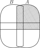
Figure 6: The corner diagram for the two separations $(A,B)$ and $(C,D)$. The separation $(A,B)$ separates vertically, while $(C,D)$ separates horizontally. The corner $A\cap C$ is shaded in grey. The middle region $A\cap B\cap C\cap D$ is called the center. The four other regions ‘linking the corners’ are called the links. Formally, they are $(A\cap B)\setminus C$, $(A\cap B)\setminus D$, $(C\cap D)\setminus A$ and $(C\cap D)\setminus B$.

In Figure 6 the separator of $(A\cap C,B\cup D)$ has the shape of an ‘L’. Hence we denote this separator by $L(A,C)$; formally, $L(A,C)$ is the intersection of $A\cap C$ and $B\cup D$. The pair consisting of $(A,B)$ and $(C,D)$ has three more corner separations, corresponding to the corners of Figure 6. These are $(A\cap D,B\cup C)$, $(B\cap C,A\cup D)$ and $(B\cap D,A\cup C)$. Analogously to $L(A,C)$ we define the separators $L(A,D)$, $L(B,C)$ and $L(B,D)$.

Observation .

$|L(A,C)|+|L(B,D)|=|A\cap B|+|C\cap D|$. ∎

Given two separations $(A,B)$ and $(C,D)$ of order at most $k$ such that $L(A,C)$ contains at most $k$ vertices, then the corner separation $(A\cap C,B\cup D)$ has order at most $k$. If additionally $P$ is a tangle of order $k+1$ such that $A$ and $C$ are big in $P$, then the side $A\cap C$ of $(A\cap C,B\cup D)$ is big in $P$; this follows from the first property of tangles as $B$, $D$ and $A\cap C$ cover all edges. We shall refer to that property of tangles as the corner property.

Another property of tangles of order $k+1$ that also follows from the property that no three small sides cover is that they are robust; that is: given two separations $(A,B)$ and $(C,D)$, where the first separation has order at most $k$ and the second separation has arbitrary finite order such that the corner separators $L(A,C)$ and $L(B,C)$ have at most $k-1$ vertices. Then if the side $C$ is big, then one of the corners $C\cap A$ or $C\cap B$ must be big.

A separation $(A,B)$ distinguishes two tangles $P_{1}$ and $P_{2}$ if the side $A$ is big in some $P_{i}$ and small in $P_{i+1}$. Note that $(A,B)$ distinguishes the $P_{i}$ if and only if $(B,A)$ distinguishes them. A separation distinguishes $P_{1}$ and $P_{2}$ efficiently if it distinguishes them and has minimal order amongst all separations distinguishing them.

4.2 Blocks and torsos

Given a set ${\cal N}$ of separations, an ${\cal N}$-block is a maximal set of vertices no two of which are separated by a separation in ${\cal N}$. For any ${\cal N}$-block $\beta$, any separation in ${\cal N}$ has (at least) one side that includes $\beta$. And $\beta$ can be written as an intersection of all these sides.

Let ${\cal N}$ be a nested set of separations of order at most $k$ and let $\beta$ be an ${\cal N}$-block of at least $k+1$ vertices. Let $P$ be a tangle of order $\ell+1$ greater than $k$. We say that the tangle $P$ lives in the block $\beta$ if for every separation $(A,B)$ of $G$ of order at most $k$ with $\beta\subseteq A$ the side $A$ is big in $P$.

Remark .

Unlike for finite graphs, not every tangle of order $k+1$ of an infinite graphs lives in an ${\cal N}$-block; indeed for tangles defined from ends the intersections of all big sides of separations in ${\cal N}$ may be empty. Subsection 4.2 shows that the definition of ‘lives in’ cannot be weakened by replacing ‘$(A,B)$ of $G$’ by ‘$(A,B)$ of ${\cal N}$’.

Example .

In this example we construct a nested set of separations of order three such that the intersections of the big sides of the tangle forms a block of size four in which the tangle does not live. We obtain the graph $G$ from a ray by attaching vertices $v$ and $w$ complete to the ray and then attaching an edge complete to $v$ and $w$, see Figure 7.

Figure 7: The graph $G$.

The tangle we focus on is the tangle of the vertex-end of $G$. The set ${\cal N}$ consists of those separations of the form $(P_{n}+v+w,G\setminus P_{n})$, where $P_{n}$ is the initial subpath of the ray of length $n$. The attached edge together with $v$ and $w$ is an ${\cal N}$-block. This ${\cal N}$-block is the intersection the big sides of separations in ${\cal N}$. Still the tangle does not live in that block in the sense that it induces a tangle in that block in the sense of Subsection 4.2 below.

The next lemma gives a criterion when tangles do live in blocks.

Lemma .

Let ${\cal N}$ be a nested set of separations of order at most $k$ and $(A,B)$ a separation of order $\ell\geq k+1$ nested with ${\cal N}$. Assume that $(A,B)$ distinguishes two tangles $P$ and $Q$ efficiently. Then there is an ${\cal N}$-block $\beta$ such that $A\cap B\subseteq\beta$ and $P$ and $Q$ live in $\beta$.

Proof.

Since the separation $(A,B)$ is nested with any separation in ${\cal N}$, no such separation separates the vertex set $A\cap B$. Note that $A\cap B$ contains at least $k+1$ vertices. Let $\beta$ be the unique ${\cal N}$-block including $A\cap B$: as above $\beta$ is unique as each separation in ${\cal N}$ has precisely one side containing $A\cap B$.

Next we show that $P$ and $Q$ live in $\beta$. For that let $(C,D)$ be a separation of order at most $k$ of $G$ with $\beta\subseteq C$. Our aim is to show that $C$ is big in $P$ and $Q$.

Suppose for a contradiction that the side $D$ is big in one of the tangles, say $P$. By symmetry, we may assume that the side $A$ is big in $P$. Since the link $(A\cap B)\setminus C$ is empty, the corner separation $(A\cap D,B\cup C)$ has order at most $k$. As $P$ has the corner property, the corner $A\cap D$ is big in $P$. On the other hand, the side $B\cup C$ must be big in $Q$ as it includes the big side $B$. Hence the corner separation $(A\cap D,B\cup C)$ distinguishes $P$ and $Q$. As this separation has order at most $k$, this is a contradiction to the efficiency of the separation $(A,B)$. Thus the side $C$ is big in both tangles $P$ and $Q$. ∎

Observation .

In the proof of Subsection 4.2 we do not make use of the whole strengths of the property of tangles that three small sides do not cover but just of the slightly weaker corner property. This will be used only once, namely in Subsection 4.2

Given a set ${\cal N}$ of separations and an ${\cal N}$-block $\beta$, the torso $G_{T}[\beta]$ of $\beta$ is obtained from $G[\beta]$ by adding an edge between any two vertices of $\beta$ that are in a common separator $A\cap B$ of some separation $(A,B)$ in ${\cal N}$. This definition is compatible with the usual definition of torso [14] in the context of tree-decompositions: if ${\cal N}$ is the set of separations corresponding to the edges of a tree-decomposition, then the vertex set of every maximal part is an ${\cal N}$-block and its torso is just the torso of that part. Moreover, we have the following.

Lemma .

Let $K$ be a component of $G-\beta$. Then any two vertices $v$ and $w$ in the neighbourhood of $K$ in $\beta$ are adjacent in the torso $G_{T}[\beta]$.

Proof.

Let $P$ be a path between $v$ and $w$ whose interior vertices are in $K$. For each separation $(C,D)$ in ${\cal N}$ its restriction to $P\cup\beta$ is $(C\cap(P\cup\beta),D\cap(P\cup\beta))$. By reversing separations in ${\cal N}$ if necessary, we may assume that $\beta\subseteq C^{\prime}$ for every restriction $(C^{\prime},D^{\prime})$. Since nestedness is preserved by restricting, there is one such restriction $(C^{\prime},D^{\prime})$ such that $D^{\prime}\setminus C^{\prime}$ includes all sets $D^{\prime\prime}\setminus C^{\prime\prime}$ for all other such restrictions $(C^{\prime\prime},D^{\prime\prime})$. As no vertex of $P-v-w$ is in $\beta$ the set $D^{\prime}\setminus C^{\prime}$ must be equal to $P-v-w$. Hence $vw$ is an edge in the torso. ∎

Lemma .

Let ${\cal N}$ be a nested set of separations of order at most $k$ and let $\beta$ be an ${\cal N}$-block. Then every component $C$ of $G-\beta$ has at most $k$ neighbours in $\beta$.

Proof.

This lemma is a well-known fact for finite graphs. We give an argument that reduces the infinite version to the finite version.

Suppose for a contradiction that some component $C$ of $G-\beta$ has at least $k+1$ vertices in its neighbourhood. Then there is a finite connected subset $C^{\prime}$ of $C$ that has a set $\beta^{\prime}$ of $k+1$ vertices of $\beta$ included in its neighbourhood. We obtain the graph $G^{\prime}$ from $G$ by deleting all vertices not in the finite vertex set $C^{\prime}\cup\beta^{\prime}$. The restrictions $(A^{\prime},B^{\prime})=(A\cap G^{\prime},B\cap G^{\prime})$ of separations $(A,B)$ in ${\cal N}$ form a nested set of separations in $G^{\prime}$. Hence we get the desired contradiction by the finite version of the lemma. This completes the proof. ∎

Remark .

Tangles have many nice properties. However, they do not always induce tangles in blocks they live in, see Subsection 4.2 below. This property will be essential for our proof strategy later on. We will overcome that problem by working within the class of ‘robust profiles’, a slight superclass of tangles.

It should be noted that robust profiles unlike tangles do not always have the following property, which makes tangles work very well with graph minors: let $G^{\prime}$ be a minor of $G$ and $T^{\prime}$ be a tangle in $G^{\prime}$, then there is a tangle in $G$ inducing $T^{\prime}$. This last statement is not used in this paper.

Example .

Consider the unique tangle of order $k+1$ on the complete bipartite graph $K_{k,k+1}$ for $k>3$. The separations of order $k$ are nested and the torso of the block in which the tangle lives is isomorphic to $K_{k}$. However, there is no tangle of order $k+1$ at $K_{k}$. (The largest tangle has order roughly $\frac{2}{3}\cdot k$.)

Robust profiles will be defined like tangles except that we weaken the property that three small sides never cover; namely we just forbid this for very particular configurations. To be precise, we define robust profiles like ‘tangles’ except that we replace the first property that three small sides never cover all edges by the following three properties.

1. no two small sides cover all edges;

2. the corner property;

3. the robustness property.

Example .

We have seen above that tangles are examples of robust profiles. A different example is the robust profile of order $k+1$ on the graph $K_{k}$.

All definitions for tangles are extended to robust profiles in the obvious way. The proof of Subsection 4.2 is the only one in the paper where we make use of the difference between tangles and robust profiles (except from those implicit places where we apply Subsection 4.2). This is necessary in order to cope with examples such as those in Subsection 4.2.

Next we define how a robust profile living in an ${\cal N}$-block $\beta$ defines a robust profile in the torso graph $G_{T}[\beta]$. The restriction of a separation $(A,B)$ of $G$ to $\beta$ is the separation $(A\cap\beta,B\cap\beta)$ of $G[\beta]$.

Lemma .

Given an ${\cal N}$-block $\beta$ and a separation $(A,B)$ nested with ${\cal N}$, the restriction of $(A,B)$ is a separation in the torso graph $G_{T}[\beta]$.

Proof.

It suffices to show that for any separation $(C,D)\in{\cal N}$ that $C\cap D$ is a subset of $A$ or $B$. This follows from the nestedness of $(A,B)$ with $(C,D)$. ∎

For any separation $(A^{\prime},B^{\prime})$ of a torso graph $G_{T}[\beta]$, there is a separation $(A,B)$ of $G$ that restricts to $(A^{\prime},B^{\prime})$ and has the same separator. Now let $P$ be a robust profile of order $\ell+1>k$ that lives in an ${\cal N}$-block $\beta$. The induced robust profile $P_{\beta}$ of $P$ at $\beta$ is defined as follows. A side $A^{\prime}$ of a separation $(A^{\prime},B^{\prime})$ of the torso graph $G_{T}[\beta]$ of order at most $\ell$ is big in $P_{\beta}$ if and only if there is a side $A$ of a separation $(A,B)$ of $G$ that restricts to $(A^{\prime},B^{\prime})$ and has the same separator such that $A$ is big in $P$.

Lemma .

Assume that a robust profile $P$ of order $\ell+1>k$ lives in the ${\cal N}$-block $\beta$. Then the induced robust profile $P_{\beta}$ is a robust profile of the torso $G_{T}[\beta]$.

Proof.

First we show that if $(A^{\prime},B^{\prime})$ is a separation of order at most $k$ of the torso, then it can have at most one big side in $P_{\beta}$.

By the component property, there is a component $K$ of the graph $G-A^{\prime}\cap B^{\prime}$ such that the side $K\cup(A^{\prime}\cap B^{\prime})$ is big in $P$. As $P$ lives in $\beta$ by assumption, the block $\beta$ is included in that side. As $\beta$ has at least $k+1$ vertices, the component $K$ contains a vertex of the block $\beta$. That is, the vertex set $K^{\prime}=K\cap\beta$ is not empty.

As $K^{\prime}$ is a restriction of a connected set, it is connected in the torso by Subsection 4.2. As the vertex set $K^{\prime}$ is disjoint from the separator $A^{\prime}\cap B^{\prime}$, there is a unique side of the separation $(A^{\prime},B^{\prime})$ that includes $K^{\prime}$, say $A^{\prime}$. Now let $(A,B)$ be any separation of $G$ that restricts to $(A^{\prime},B^{\prime})$ and has the separator $A^{\prime}\cap B^{\prime}$. Since $K$ includes $K^{\prime}$, the set $K$ cannot be included in $B$. So it is included in $A$. So $A$ must be big in $P$ as it includes a big side. In particular $B$ is small in $P$. Since $(A,B)$ is arbitrary, $B^{\prime}$ cannot be big.

To see that $P_{\beta}$ has the component property, let $X$ be a set of at most $\ell$ vertices of the torso. Let $K$ be a component of $G-X$ such that the side $(K\cup X)$ of $(K\cup X,G\setminus K)$ is big in $P$. Let $K^{\prime}=K\cap\beta$, which is connected in the torso by Subsection 4.2.

Next we show that $K^{\prime}$ is not empty. Suppose not for a contradiction. Then the component $K$ contains no vertex of the block $\beta$. So $K$ is a component of $G-\beta$. By Subsection 4.2, the component $K$ has at most $k$ neighbours in the block $\beta$. So the separation $(K\cup N(K),G\setminus K)$ has order at most $k$. As $P$ lives in $\beta$, the side $G\setminus K$ is big in $P$. This is a contradiction to the fact that $P$ is a robust profile as the side $K\cup N(K)$ is big in $P$. Hence the set $K^{\prime}$ must be nonempty.

Let $K^{\prime\prime}$ be the component of the torso $G_{T}[\beta]$ without $X$ including the connected nonempty set $K^{\prime}$. Then $K^{\prime\prime}\cup X$ is big in the induced robust profile. So $P_{\beta}$ has the component property.

It remains to show that two small sides in the torso do not cover and to show the corner property and robustness for $P_{\beta}$. To see the first, suppose for a contradiction that the torso is covered by two small sides. We observe that if the edge set of a complete graph is covered by two subgraphs, then one of these subgraphs must include the whole vertex set of the complete graph. Hence by Subsection 4.2 for each component $K$ of $G$ without the torso, there is one of the sides that includes the whole neighbourhood of $K$. So we can assign each component $K$ to a side that includes its neighbourhood. Each of the two covering sides together with its assigned components forms a side of a separation of order at most $\ell$ in the graph $G$. As this side restricts to a small side in the torso, it must be small in the original robust profile $P$ by definition of the induced robust profile and by the first part of the proof. Hence the graph $G$ is covered by two sides that are small in $P$, which is not possible as $P$ is a robust profile $P$.

Having shown that two small sides cannot cover in the torso, it remains to verify the the corner property and robustness for $P_{\beta}$. In a nutshell, they are both true as taking the corner separation commutes with taking the torso. In detail, let $(A^{\prime},B^{\prime})$ and $(C^{\prime},D^{\prime})$ be two separations of the torso of order at most $\ell$ and assume that their corner separator $L(A^{\prime},C^{\prime})$ contains at most $\ell$ vertices. Then there are separations $(A,B)$ and $(C,D)$ of $G$ that restrict to $(A^{\prime},B^{\prime})$ and $(C^{\prime},D^{\prime})$ and have the same separator; in particular, all vertices of the separators $A\cap B$ and $C\cap D$ are vertices of the torso. Hence the corner separator $L(A,C)$ is equal to the corner separator $L(A^{\prime},C^{\prime})$. So the corner property for $P_{\beta}$ follows from the corner property for $P$. Similarly robustness for $P_{\beta}$ follows from robustness for $P$. So $P_{\beta}$ is a robust profile of the torso. ∎

Observation .

Subsection 4.2 is true with ‘tangle’ replaced by ‘robust profile’.

Proof.

This follows from Subsection 4.2. ∎

4.3 Extending separations of the torsos

The aim of this subsection is to explain how for a given nested set ${\cal N}$ of separations and a torso of an ${\cal N}$-block, a nested set of separations of the torso can be extended to a nested set of separations of the whole graph that is nested with ${\cal N}$. This is more technical and hence more complicated as one might expect. Indeed, extending a single separation of the torso is quite easy – but it is not uniquely defined. We have to make some choices. If we make these choices arbitrarily for two nested separations, it could happen that their extensions are no longer nested, see Subsection 4.3 below.

Throughout this subsection we fix a nested set ${\cal N}$ of separations and an ${\cal N}$-block $\beta$. For each separation $(C,D)\in{\cal N}$ at least one of the sides $C$ and $D$ includes $\beta$. Let ${\cal N}_{\beta}$ consist of those separations $(C,D)$ such that $\beta$ is included in $C$ and $(C,D)$ or $(D,C)$ is in ${\cal N}$.

Given a separation $(A,B)$ of the torso $G_{T}[\beta]$, one way to ‘extend’ $(A,B)$ to a separation of $G$ is to decide for each component of $G-\beta$, whether we put it on the $A$-side or on the $B$-side. Below we define what it means when such a component is ‘forced’. Informally, it is forced when we must put it on the $A$-side in order to extend $(A,B)$ to a separation of $G$.

A component $K$ of $G-\beta$ is forced at step $1$ by $(A,B)$ if one of its vertices has a neighbour in $A\setminus B$. A separation $(C,D)\in{\cal N}_{\beta}$ is forced at step $2n+2$ if there is a component $K$ forced at step $2n+1$ that contains a vertex of $D\setminus C$. A component $K$ of $G-\beta$ is forced at step $2n+1$ for $n>0$ if there is a separation $(C,D)\in{\cal N}_{\beta}$ forced at step $2n$ so that $K$ contains a vertex of $D\setminus C$. An alternative definition of ‘forcing’ is the following.

Example .

We define the bipartite graph whose left side are the components of $G-\beta$ and whose right side are the separations in ${\cal N}_{\beta}$. We add an edge between a component $K$ and a separation $(C,D)$ if $K$ contains a vertex of $D\setminus C$. A component (or separation) is forced if and only if its connected component in this bipartite graph contains a component forced at step one. We will not use the fact that this definition is equivalent in our proofs.

The following lemma implies that if a component is forced at some step, it is forced at step one or three; and if a separation is forced, it is forced at step two or four.

Lemma .

Let $(C,D)$ be a separation in ${\cal N}_{\beta}$ forced by $(A,B)$. There is some $(C^{\prime},D^{\prime})$ in ${\cal N}_{\beta}$ forced by $(A,B)$ with $D\setminus C\subseteq D^{\prime}\setminus C^{\prime}$ such that some vertex of $C^{\prime}\cap D^{\prime}$ is in $A\setminus B$.

Proof.

Let $2n$ be the smallest step at which $(C,D)$ is forced. We prove Subsection 4.3 by induction on $n$.

The base case is that $2n=2$. Let $K$ be a component forced at step one ‘forcing’ $(C,D)$; here we say that $K$ forces the separation $(C,D)$ if there is a vertex of $K$ in $D\setminus C$ and $(C,D)$ is not forced at an earlier step than $K$.

As $K$ is forced at step one, there is a vertex $v$ of $K$ that has a neighbour $w$ in $A\setminus B$. As $v$ is not in $\beta$, there is a separation $(E,F)$ in ${\cal N}_{\beta}$ such that $v$ is in $F\setminus E$. As $w$ is in $\beta$, it is in $E$. As it has a neighbour in $F\setminus E$, it also must be in $F$.

We call a separation $(E^{\prime},F^{\prime})$ a candidate if the separator $E^{\prime}\cap F^{\prime}$ contains a vertex of $A\setminus B$ and $F^{\prime}\setminus E^{\prime}$ contains a vertex of the component $K$. For example, the separation $(E,F)$ is a candidate. To conclude the base case, we show the following.

Sublemma .

Assume that there is a candidate. Then there is a separation $(C^{\prime},D^{\prime})$ in ${\cal N}_{\beta}$ forced by $(A,B)$ with $D\setminus C\subseteq D^{\prime}\setminus C^{\prime}$ such that some vertex of $C^{\prime}\cap D^{\prime}$ is in $A\setminus B$.

Proof.

We pick a candidate $(E,F)$. Let $w$ be a vertex of the separator $E\cap F$ in $A\setminus B$. If the vertex $w$ was in the separator $C\cap D$, the lemma would be true with ‘$(C,D)$’ in place of ‘$(C^{\prime},D^{\prime})$’. Hence we may assume that the vertex $w$ of $\beta$ is not in the side $D$ as $\beta\subseteq C$. So the vertex $w$ is in the link $(E\cap F)\setminus D$. So from the nestedness of $(C,D)$ and $(E,F)$ it follows that either $D\setminus C\subseteq F\setminus E$ or else $D\setminus C$ and $F\setminus E$ are vertex-disjoint.

Our aim is to construct a candidate $(E,F)$ that satisfies the first condition $D\setminus C\subseteq F\setminus E$. Let $u$ and $v$ be vertices of $K$ that are in $D\setminus C$ and $F\setminus E$, respectively (such vertices exist as we may assume that $D\setminus C$ is not empty and $(E,F)$ is a candidate).. Let $P$ be a path from the vertex $u$ to vertex $v$ included in the component $K$ of $G-\beta$. By assumption for every vertex $x$ on $P$, there is a separation $(C_{x},D_{x})\in{\cal N}_{\beta}$ with $x\in D_{x}\setminus C_{x}$. If possible we choose the separation $(C_{x},D_{x})$ such that the vertex $w$ is in the separator (in that case it is a candidate).

Our goal is to show that it is possible to choose the separation $(C_{u},D_{u})$ at $u$ such that the vertex $w$ is in the separator. Indeed, then we can use the nestedness of $(C_{u},D_{u})$ and $(C,D)$ to deduce as above that $D\setminus C\subseteq D_{u}\setminus C_{u}$ or else $D\setminus C$ and $D_{u}\setminus C_{u}$. However, here the second outcome is not possible as the vertex $u$ is in the intersection of these two sets.

Suppose for a contradiction that such a choice for $(C_{u},D_{u})$ is not possible. Let $x$ be the vertex on the path $P$ nearest to $u$ such that the vertex $w$ is in its separator $C_{x}\cap D_{x}$. Let $y$ be the neighbour of $x$ on $P$ nearer to $u$, which exists as $x\neq u$. Then the vertex $w$ is in the link $(C_{x}\cap D_{x})\setminus D_{y}$. As above we deduce from the nestedness of the separations $(C_{x},D_{x})$ and $(C_{y},D_{y})$, that either $D_{y}\setminus C_{y}\subseteq D_{x}\setminus C_{x}$ or else $D_{y}\setminus C_{y}$ and $D_{x}\setminus C_{x}$ are vertex-disjoint. Since we cannot choose $(C_{x},D_{x})$ in place of $(C_{y},D_{y})$, the first outcome is impossible. The second outcome is not possible either as the vertex $x\in D_{x}\setminus C_{x}$ is adjacent to the vertex $y\in D_{y}\setminus C_{y}$. So this is the desired contradiction. Hence we can choose $(C_{u},D_{u})$ such that it is a candidate, which completes the proof as shown above. ∎

So the base case follows from Subsection 4.3 and the fact that $(E,F)$ is a candidate.

Now let $n>1$ and assume that we already proved Subsection 4.3 for separations $(E,F)$ forced at some step before $2n$. Let $(C,D)$ be a separation in ${\cal N}_{\beta}$ forced at step $2n$. Let $K$ force $(C,D)$. Let $(C_{1},D_{1})$ be a separation forcing $K$, which exists as $n>1$. By the induction hypothesis, there is a separation $(C_{2},D_{2})$ in ${\cal N}_{\beta}$ forced by $(A,B)$ with $D_{1}\setminus C_{1}\subseteq D_{2}\setminus C_{2}$ such that some vertex $w$ of $C_{2}\cap D_{2}$ is in $A\setminus B$. As $D_{1}\setminus C_{1}\subseteq D_{2}\setminus D_{2}$, there is a vertex $v$ of $K$ that is in $D_{2}\setminus C_{2}$. So $(C_{2},D_{2})$ is a candidate. So the induction step follows from Subsection 4.3. This completes the proof. ∎

Lemma .

For any separation $(A,B)$ of the torso, no component $K$ of $G-\beta$ is forced by both $(A,B)$ and $(B,A)$.

Proof.

As any component of $G-\beta$ forces some separation in ${\cal N}_{\beta}$, it suffices to show that no separation $(C,D)$ in ${\cal N}_{\beta}$ is forced by both $(A,B)$ and $(B,A)$. Suppose for a contradiction that there is such a separation $(C,D)$.

By Subsection 4.3, there is a separation $(C^{\prime},D^{\prime})\in{\cal N}_{\beta}$ forced by $(A,B)$ with $D\setminus C\subseteq D^{\prime}\setminus C^{\prime}$ such that some vertex $v$ of $C^{\prime}\cap D^{\prime}$ is in $A\setminus B$. As $D^{\prime}\setminus C^{\prime}$ is a superset of $D\setminus C$, the separation $(C^{\prime},D^{\prime})$ is also forced by $(B,A)$. Applying Subsection 4.3 to $(C^{\prime},D^{\prime})$ and to $(B,A)$, yields a separation $(C^{\prime\prime},D^{\prime\prime})$ with $D^{\prime}\setminus C^{\prime}\subseteq D^{\prime\prime}\setminus C^{\prime\prime}$ such that some vertex $w$ of $C^{\prime\prime}\cap D^{\prime\prime}$ is in $B\setminus A$. Since the vertex $v$ is in $\beta$, it must be in $C^{\prime\prime}$. As $D^{\prime\prime}$ includes $D^{\prime}$, it also is in $D^{\prime\prime}$. In short, $v$ is in the separator $C^{\prime\prime}\cap D^{\prime\prime}$.

Hence the separation $(C^{\prime\prime},D^{\prime\prime})$ witnesses that $vw$ is an edge of the torso. As $v$ is in $A\setminus B$ and $w$ is in $B\setminus A$, we deduce that $(A,B)$ cannot be a separation of the torso. That is the desired contradiction. ∎

Having finished the proof of Subsection 4.3, we now define naive extensions of separations of the torso, explain why they are not quite the object we need and define extensions of nested sets of separations of the torso.

Given a separation $(A,B)$ of the torso, the side $\hat{A}$ is obtained from $A$ by adding all components $K$ of $G-\beta$ that are forced at some step. We obtain $\widehat{\hat{B}}$ from $B$ by adding all components $K$ that are not forced at any step. Note that $\widehat{\hat{B}}=B\cup(G\setminus\hat{A})$. We define the naive extension of $(A,B)$, denoted by $\widehat{(A,B)}$, to be $(\hat{A},\widehat{\hat{B}})$. This construction ensures that $\widehat{(A,B)}$ is a separation of $G$ that restricts to $(A,B)$.

Remark .

We chose the notation ‘$\widehat{\hat{B}}$’ instead of simply ‘$\hat{B}$’ as the term $\hat{A}$ for the separation $(A,B)$ and the term ‘$\widehat{\hat{A}}$’ for the separation $(B,A)$ need not a priori agree – and in fact they do not agree for $(A,B)$ defined as in Subsection 4.3.

In particular, the reverse separation of $\widehat{(A,B)}$ is in general not equal to $\widehat{(B,A)}$.

Observation .

Given two separations $(A,B)$ and $(X,Y)$ of the torso, if $(A,B)\leq(X,Y)$, then $\widehat{(A,B)}\leq\widehat{(X,Y)}$. ∎

Observation .

Let $(A,B)$ be a separation of the torso and $(C,D)\in{\cal N}_{\beta}$ be a proper separation. Then $\widehat{(A,B)}$ or its reverse separation $(\widehat{\hat{B}},\hat{A})$ is $\leq(C,D)$.

In particular, $\widehat{(A,B)}$ is nested with every proper separation of ${\cal N}$.

Proof.

First assume that the separation $(C,D)$ is forced at some step. Then $D\setminus C$ is a subset of $\hat{A}$. Since the separator $A\cap B$ of the separation $(\widehat{\hat{B}},\hat{A})$ is a subset of the block $\beta$, which is included in the side $C$, we conclude that $D\setminus C$ is a subset of $\hat{A}\setminus\widehat{\hat{B}}$. As in the proof of Section 2 one combines this with the assumption that the separation $(C,D)$ is proper to deduce that $(D,C)\leq\widehat{(A,B)}$.

Hence it remains to consider the case that the separation $(C,D)$ is not forced at any step. Analoguously as above, one shows that $(D,C)\leq(\widehat{\hat{B}},\hat{A})$ in that case. So $\widehat{(A,B)}$ or its reverse separation $(\widehat{\hat{B}},\hat{A})$ is $\leq(C,D)$.

∎

Subsection 4.3 gives an example of nested separations $(A,B)$ and $(C,D)$ of the torso $G_{T}[\beta]$ whose naive extensions $\widehat{(A,B)}$ and $\widehat{(C,D)}$ are not nested.

Example .

Let $G$ be the labelled graph depicted in Figure 8. The set ${\cal N}$ consists of the separation of order one and its reverse. Then the torso is $G-6$. We define $A=\{1,2,3,5\}$, $B=\{3,4,5\}$, $C=\{2,3,4,5\}$, $D=\{1,2,5\}$. Then $(A,B)$ and $(C,D)$ are nested but not $\widehat{(A,B)}$ and $\widehat{(C,D)}$.

Figure 8: The graph $G$ is obtained by from a triangle by attach two more triangles at distinct edges and by then attaching a leaf at the unique vertex of degree four.

Examples like Subsection 4.3 motivate the slightly technical definition of $\widetilde{{\cal L}}$ below. Given a nested set ${\cal L}$ of separations of $G_{T}[\beta]$, the extension $\widetilde{{\cal L}}$ of ${\cal L}$ (depending on a well-order $({(A_{\alpha},B_{\alpha})}\mid\alpha\in\kappa)$ of ${\cal L}$) is the set $\{\widetilde{(A_{\alpha},B_{\alpha})}\mid(A_{\alpha},B_{\alpha})\in{\cal L}\}$, where the extension $\widetilde{(A,B)}$ of $(A,B)$ is defined as follows: for the smallest element $(A_{0},B_{0})$ of the well-order, we just let $\widetilde{(A_{0},B_{0})}=\widehat{(A_{0},B_{0})}$.

Assume that we already defined $\widetilde{(A_{\alpha},B_{\alpha})}$ for all $\alpha<\gamma$. A component $K$ of $G-\beta$ is $\gamma$-forced if there is some $\alpha<\gamma$ such that $K$ is a subset of $\tilde{B}_{\alpha}$ and $(B_{\alpha},A_{\alpha})\leq(A_{\gamma},B_{\gamma})$. We obtain $\tilde{A}_{\gamma}$ from $A_{\gamma}$ by adding all components $K$ of $G-\beta$ that are forced by $(A_{\gamma},B_{\gamma})$ or are $\gamma$-forced. We obtain $\tilde{B}_{\gamma}$ from $B_{\gamma}$ by adding all other components. The extension $\widetilde{(A_{\gamma},B_{\gamma})}$ of $(A_{\gamma},B_{\gamma})$ is defined to be $(\tilde{A}_{\gamma},\tilde{B}_{\gamma})$.

Example .

The nested set ${\cal L}=\{(A,B),(C,D)\}$ defined in Subsection 4.3 has different extensions $\widetilde{\cal L}$ depending on which well-order we choose.

Observation .

The extension $(\tilde{A}_{\gamma},\tilde{B}_{\gamma})$ is a separation.

Proof.

It suffices to show that any component $K$ of $G-\beta$ included in $\tilde{A}_{\gamma}$ is not forced by $(B_{\gamma},A_{\gamma})$. By Subsection 4.3, we may assume that $K$ is $\gamma$-forced. As any class of ordinals has a least element, there is some $\alpha$ minimal such that $K$ is a subset of $\tilde{B}_{\alpha}$ and $(B_{\alpha},A_{\alpha})\leq(A_{\gamma},B_{\gamma})$. In particular, $K$ is not forced by $(A_{\alpha},B_{\alpha})$. As $B_{\gamma}\setminus A_{\gamma}$ is a subset of $A_{\alpha}\setminus B_{\alpha}$, we deduce that $K$ cannot be forced by $(B_{\gamma},A_{\gamma})$. ∎

Observation .

Any separation $(A,B)$ of the torso has the same separator as its extension $\widetilde{(A,B)}$.∎

Observation .

For any two separations $(A,B)$ and $(B,A)$ in ${\cal L}$, the extension $\widetilde{(A,B)}$ is the reverse of $\widetilde{(B,A)}$.

Proof.

We may assume that $(A,B)=(A_{\alpha},B_{\alpha})$ and $(B,A)=(A_{\gamma},B_{\gamma})$ for some $\alpha<\gamma$. It suffices to show that $\tilde{B}_{\alpha}=\tilde{A}_{\gamma}$. By construction $\tilde{B}_{\alpha}\subseteq\tilde{A}_{\gamma}$. Suppose for a contradiction that $\tilde{B}_{\alpha}$ is a proper subset of $\tilde{A}_{\gamma}$. Then there is a component $K$ that is included in $\tilde{A}_{\alpha}$ and in $\tilde{A}_{\gamma}$. We split into four cases and derive a contradiction in each of them.

Case 1A: $K$ is forced by $(A,B)$ and $(B,A)$. This is impossible by Subsection 4.3.

Case 1B: $K$ is forced by $(A,B)$ and $\gamma$-forced. So there is some ordinal $\delta<\gamma$ such that $K$ is a subset of $\tilde{B}_{\delta}$ and $(B_{\delta},A_{\delta})\leq(A_{\gamma},B_{\gamma})$. Then $(A,B)\leq(A_{\delta},B_{\delta})$. So $K$ is forced by $(A_{\delta},B_{\delta})$. So it cannot be a subset of $\tilde{B}_{\delta}$, a contradiction.

Case 2A: $K$ is $\alpha$-forced and forced by $(B,A)$. This case is analogue to Case 1B.

Case 2B: $K$ is $\alpha$-forced and $\gamma$-forced. So there is some ordinal $\delta<\alpha$ such that $K$ is a subset of $\tilde{B}_{\delta}$ and $(B_{\delta},A_{\delta})\leq(A_{\alpha},B_{\alpha})$; and there is some ordinal $\epsilon<\gamma$ such that $K$ is a subset of $\tilde{B}_{\epsilon}$ and $(B_{\epsilon},A_{\epsilon})\leq(A_{\gamma},B_{\gamma})$. To summarise:

$$(B_{\delta},A_{\delta})\leq(A,B)\leq(A_{\epsilon},B_{\epsilon})$$

If $\delta<\epsilon$, then the component $K$ is $\epsilon$-forced and hence not in $\tilde{B}_{\epsilon}$, which is impossible. Similarly, we also cannot have $\delta>\epsilon$. So $\delta=\epsilon$. But then the component $K$ is included in the sides $B_{\delta}$ and $A_{\delta}\supseteq B_{\epsilon}$, which is the desired contradiction. ∎

Observation .

For any two separations $(A_{\alpha},B_{\alpha})$ and $(A_{\gamma},B_{\gamma})$ in the nested set ${\cal L}$, their extensions $\widetilde{(A_{\alpha},B_{\alpha})}$ and $\widetilde{(A_{\gamma},B_{\gamma})}$ are nested.

Proof.

By symmetry we may assume that $\alpha<\gamma$. If $B_{\alpha}$ is a subset of $A_{\gamma}$, it follows immediately from the definitions that $\widetilde{(B_{\alpha},A_{\alpha})}\leq\widetilde{(A_{\gamma},B_{\gamma})}$. If $A_{\alpha}$ is a subset of $A_{\gamma}$, then $\widetilde{(A_{\alpha},B_{\alpha})}\leq\widetilde{(A_{\gamma},B_{\gamma})}$ by construction.

The other two cases can be deduced using Subsection 4.3 as follows. First assume that $(B_{\gamma},A_{\gamma})$ is not in ${\cal L}$. Then we add that separation at the end of the well-order for ${\cal L}$. Now we apply the above argument to $(A_{\alpha},B_{\alpha})$ and $(B_{\gamma},A_{\gamma})$. Hence $\widetilde{(A_{\alpha},B_{\alpha})}$ and $\widetilde{(B_{\gamma},A_{\gamma})}$ are nested. By Subsection 4.3 also $\widetilde{(A_{\alpha},B_{\alpha})}$ and $\widetilde{(A_{\gamma},B_{\gamma})}$ are nested.

The same argument works if $(B_{\gamma},A_{\gamma})$ is in ${\cal L}$ but in the well-order after position $\alpha$. If it is before $\alpha$, we replace $(A_{\alpha},B_{\alpha})$ or $(A_{\gamma},B_{\gamma})$ by their reverses if they appear before in the well-order and then do the above argument. This implies the desired result by Subsection 4.3. ∎

Observation .

For any separation $(A,B)\in{\cal L}$, its extension $\widetilde{(A,B)}$ is nested with every proper separation in ${\cal N}$.

Proof.

Let $(A,B)=(A_{\gamma},B_{\gamma})$. We say that a separation $(C,D)$ of ${\cal N}_{\beta}$ is $\gamma$-forced if there is some component $K$ of $G-\beta$ that contains a vertex of $D\setminus C$ and is $\gamma$-forced or forced by $(A_{\gamma},B_{\gamma})$.

We claim that if a separation of ${\cal N}_{\beta}$ is $\gamma$-forced, then every component of $G-\beta$ that contains a vertex of $D\setminus C$ is $\gamma$-forced or forced by $(A_{\gamma},B_{\gamma})$. Indeed, if any such component is forced by a separation of the nested set ${\cal L}$, then all of these components are. Hence this follows by transfinite induction on the well-order of ${\cal L}$.

Using this, we can argue as in the proof of Subsection 4.3. ∎

Lemma .

Let ${\cal N}$ be a nested set of proper separations and let $\beta$ and $\gamma$ be distinct ${\cal N}$-block. Let ${\cal L}_{\beta}$ and ${\cal L}_{\gamma}$ be nested sets of separations of $G_{T}[\beta]$ and $G_{T}[\gamma]$, respectively. Then $\widetilde{{\cal L}}_{\beta}$ is a set of nested separations. For any separations $(A,B)\in{\cal L}_{\beta}$ and $(C,D)\in{\cal L}_{\gamma}$, their extensions $\widetilde{(A,B)}$ and $\widetilde{(C,D)}$ are nested. Moreover, they are nested with every separation in ${\cal N}$.

Proof.

The set $\widetilde{{\cal L}}_{\beta}$ is nested by Subsection 4.3. The ‘Moreover’-part follows from Subsection 4.3. So it remains to show that for any separations $(A,B)\in{\cal L}_{\beta}$ and $(C,D)\in{\cal L}_{\gamma}$, the extensions $\widetilde{(A,B)}$ and $\widetilde{(C,D)}$ are nested.

Since the blocks $\beta$ and $\gamma$ are distinct, there is a separation $(E,F)$ of ${\cal N}$ such that one side includes the block $\beta$ and the other side includes the block $\gamma$. By symmetry we may assume that $\beta$ is included in $E$ and $\gamma$ is included in $F$. By Subsection 4.3 $\widetilde{(A,B)}$ is nested with $(E,F)$. An argument as in the proof of Subsection 4.3 gives that $F\setminus E$ is included in $B\setminus A$ or $A\setminus B$. So either $\widetilde{(A,B)}$ or its reverse is $\leq(E,F)$.

By Subsection 4.3 it would be enough to show that one of $\widetilde{(A,B)}$ or its reverse is nested with $\widetilde{(C,D)}$. Hence by replacing ‘$(A,B)$’ by $(B,A)$ if necessary, we assume that $\widetilde{(A,B)}\leq(E,F)$. Similarly, one may assume that $(E,F)\leq\widetilde{(C,D)}$. Combining this yields that $\widetilde{(A,B)}$ and $\widetilde{(C,D)}$ are nested. ∎

Observation .

Let $\beta$, $P$, $Q$, $P_{\beta}$ and $Q_{\beta}$ as in Subsection 4.2. Let ${\cal L}$ be a nested set of separations in $G_{T}[\beta]$. If a separation $(C,D)\in{\cal L}$ distinguishes the induced robust profiles $P_{\beta}$ and $Q_{\beta}$ in the torso $G_{T}[\beta]$, then the extension $\widetilde{(C,D)}$ distinguishes the robust profiles $P$ and $Q$.

Proof.

By symmetry we may assume that $C$ is big in $P_{\beta}$ and $D$ is big in $Q_{\beta}$. As $P_{\beta}$ is a robust profile by Subsection 4.2, the component property yields that there is a component $K_{1}$ of $\beta-(C\cap D)$ such that $K_{1}\cup(C\cap D)$ is big in $P_{\beta}$. So $K_{1}$ is a subset of $C$.

The extension $\widetilde{(C,D)}=(\tilde{C},\tilde{D})$ has the separator $C\cap D$ by Subsection 4.3. Let $K_{1}^{\prime}$ be the components of $G-C\cap D$ such that the side $K_{1}^{\prime}\cup(C\cap D)$ is big in $P$. As $P_{\beta}$ is induced by $P$, it must be that $K_{1}$ contains a vertex of $K_{1}^{\prime}$. In particular $K_{1}^{\prime}$ cannot be a subset of $\tilde{D}$. So it must be a subset of $\tilde{C}$. Hence $\tilde{C}$ is big in $P$. Similarly one shows that $\tilde{D}$ is big in $Q$. So the extension $\widetilde{(C,D)}$ distinguishes the robust profiles $P$ and $Q$. ∎

4.4 Miscellaneous

The lemmas summarised in this subsection are well-known.

Lemma .

Let $(A,B)$ and $(C,D)$ be proper separations such that $A\setminus B$ is connected and does not intersect the separator $C\cap D$. Then $(A,B)$ and $(C,D)$ are nested.

Proof.

By the definition of nestedness, it suffices to show that $(A,B)\leq(C,D)$ or $(A,B)\leq(D,C)$. As the connected set $A\setminus B$ does not intersect the separator $C\cap D$, it is included in $C\setminus D$ or $D\setminus C$. By symmetry, we may assume that is is included in $C\setminus D$. So $A\setminus B$ is included in $C\setminus D$. Hence by Section 2 $(A,B)$ and $(C,D)$ are nested. ∎

Lemma ([9, Lemma 2.2]).

Let $(A,B)$, $(C,D)$ and $(E,F)$ be proper separations such that first $(A,B)$ and $(C,D)$ are not nested and second the corner separation $(A\cap C,B\cup D)$ is not nested with $(E,F)$. Then $(E,F)$ is not nested with $(A,B)$ or $(C,D)$.

A separation $(A,B)$ of a graph $G$ is tight if every component of $G$ without the separator $A\cap B$ has the whole separator $A\cap B$ in its neighbourhood.

Lemma .

Let $(A,B)$ be a separation of order at most $k$. Let $(C,D)$ be a tight separation such that the graph $G$ without the separator $C\cap D$ has at least $k+1$ components. Then one of the links $(C\cap D)\setminus A$ or $(C\cap D)\setminus B$ is empty.

Proof.

Suppose not for a contradiction, then there are vertices $v\in(C\cap D)\setminus A$ and $w\in(C\cap D)\setminus B$. Then $v$ and $w$ are in the neighbourhood of every component of $G$ without the separator $C\cap D$. Thus there are $k+1$ internally disjoint paths from $v$ to $w$. All of these paths contain vertices of the separator $A\cap B$. This contradicts the assumption that the separator $A\cap B$ contains at most $k$ vertices. ∎

Given two vertices $v$ and $w$, a separator $S$ separates $v$ and $w$ minimally if each component of $G-S$ containing $v$ or $w$ has the whole of $S$ in its neighbourhood.

Lemma ([24, Statement 2.4]).

Given vertices $v$ and $w$ and $k\in{\mathbb{N}}$, there are only finitely many distinct separators of size at most $k$ separating $v$ from $w$ minimally.

5 Distinguishing the tangles

The aim in this section is to construct for any graph a nested set of separations of finite order that distinguishes any two vertex-ends efficiently, which is needed in the proof of Theorem 1. A related result is proved in [11]. Actually, we shall prove the stronger statement that there is a nested set ${\cal N}$ of separations that distinguishes any two tangles efficiently. A simplified version of this proof for finite graphs has been published in [7].

Overview of the proof

We shall construct the set ${\cal N}$ as an ascending union of sets ${\cal N}_{k}$ one for each $k\in{\mathbb{N}}$, where ${\cal N}_{k}$ is a nested set of separations of order at most $k$ distinguishing efficiently any two tangles of order $k+1$, see Figure 9.

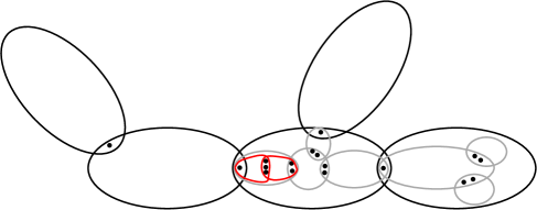
Figure 9: The tree-decomposition corresponding to the nested set ${\cal N}_{1}$ is indicated by black parts. In torsos of that tree-decomposition, in grey we indicated a tree-decomposition for ${\cal N}_{2}$. In each torso of that tree-decomposition we have a further tree-decomposition given by ${\cal N}_{3}$, etc.

Any two tangles of order $k+2$ that are not distinguished by ${\cal N}_{k}$ will live in the same ${\cal N}_{k}$-block. We obtain ${\cal N}_{k+1}$ from ${\cal N}_{k}$ by adding for each ${\cal N}_{k}$-block $\beta$ a nested set $\widetilde{{\cal N}_{k+1}(\beta)}$ that distinguishes efficiently any two tangles of order $k+2$ living in $\beta$. Working in the torsos $G_{T}[\beta]$ will ensure that the sets $\widetilde{{\cal N}_{k+1}(\beta)}$ for different blocks $\beta$ will be nested with each other.

Summing up, we are left with the task of finding in these torso graphs $G_{T}[\beta]$ a nested set distinguishing efficiently tangles of order $k+2$. Theorem 5.1 deals with this problem if the torso $G_{T}[\beta]$ is ‘nice enough’. In order to make all torso graphs nice enough, we first do an additional step in which we enlarge ${\cal N}_{k}$ a little bit so that for the larger nested set the new torso graphs are the old ones with the junk cut off. The main lemma for this enlargement is Section 5.

As explained in Subsection 4.2 and Subsection 4.2, for such a torso-approach to work we need to work within the superclass of robust profiles that includes all the tangles (instead of just the tangles).

Finishing the overview, we first state Theorem 5.1 and Section 5 and introduce the necessary definitions for that.

For any robust profile $P$ and $k\in{\mathbb{N}}$, its restriction $P_{k}$ to $k$ consists of those separations in $P$ that have order at most $k$. The order of $P_{k}$ is the minimum of $k+1$ and the order of $P$. A (robust) profile set is a set of robust profiles that is closed under restrictions. Until the end of Subsection 5.2, we fix a graph $G$, a number $k\in{\mathbb{N}}\cup\{\infty\}$ and a profile set ${{\cal P}}$.

A nested set ${\cal N}$ of separations is extendable (for ${{\cal P}}$) if for any two (distinct) robust profiles in ${{\cal P}}$ of the same order, there is some separation distinguishing these two robust profiles efficiently that is nested with ${\cal N}$.

A separation is relevant (for a number $k\in{\mathbb{N}}\cup\{\infty\}$, a graph $G$ and a profile set ${{\cal P}}$) if it has order at most $k$ and it distinguishes two robust profiles in ${{\cal P}}$ efficiently – in particular, it has finite order. We denote the set of all relevant separations by $R(k,{{\cal P}},G)$.

Given a separation $(A,B)$, a component $C$ of $G-A\cap B$ is degenerated if its neighbourhood $N(C)$ is a proper subset of the separator $A\cap B$, see Figure 10.

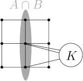
Figure 10: The separator $A\cap B$ is indicated in grey and has size three. The component $K$ of $G-A\cap B$ has only two neighbours in the separator $A\cap B$ and thus is degenerated.

A separation is degenerated relative to $(A,B)$ if it is of the form $(C\cup N(C),G\setminus C)$, where $C$ is a degenerated component of $G-A\cap B$. Given a set ${{\cal S}}$ of separations, its degenerator is the set of separations that are degenerated relative to some separation in ${{\cal S}}$. We denote the degenerator of the set $R(k,{{\cal P}},G)$ of relevant separations by $S(k,{{\cal P}},G)$. If it is clear from the context what $G$ is, we shall just write $R(k,{{\cal P}})$ or $S(k,{{\cal P}})$, or even just $R(k)$ or $S(k)$.

Example .

Every relevant separation in $R(k)$ is tight if and only if $S(k)$ is empty.

Theorem 5.1.

Let $k\in{\mathbb{N}}$. Assume that $S(k)=\emptyset$ and $R(k-1)=\emptyset$. Let ${\cal N}$ be any nested subset of $R(k)$ that is inclusion-wise maximal.

Then ${\cal N}$ distinguishes any two robust profiles of order $k+1$ in ${{\cal P}}$ efficiently and is extendable.

Lemma .

If $R(k-1)$ is empty, then the degenerator $S(k)$ is a nested extendable set of separations.

5.1 Proof of Section 5.

In this subsection we prove Section 5. First we need some preparation.

A separation $(A,B)$ pre-disqualifies a separation $(C,D)$ if the order of $(C,D)$ is strictly larger than the sizes $|L(A,C)|$ and $|L(B,C)|$ of corner separators. A separation $(A,B)$ disqualifies a separation $(C,D)$ if it pre-disqualifies $(C,D)$ or its reverse $(D,C)$.

The following lemma shows that relevant separations cannot be disqualified.

Lemma .

If $(C,D)$ distinguishes robust profiles $P_{1}$ and $P_{2}$ efficiently, then no separation $(A,B)$ disqualifies $(C,D)$.

Proof.

We may assume that $C$ is big in $P_{1}$ and $D$ is big in $P_{2}$. Suppose for a contradiction that some separation $(A,B)$ pre-disqualifies $(C,D)$.

So the order of $(C,D)$ is strictly larger than $|L(A,C)|$ and $|L(B,C)|$. The side $B\cup D$ of the corner separation $(A\cap C,B\cup D)$ is big in the robust profile $P_{2}$ as it includes a big side. By the efficiency of $(C,D)$, this corner separation cannot distinguish $P_{1}$ and $P_{2}$. Thus $A\cap C$ is small in $P_{1}$. A similar argument shows that also the corner $B\cap C$ must be small in $P_{1}$. This violates the robustness of $P_{1}$. This is a contradiction to the assumption that $P_{1}$ is a robust profile. Hence $(A,B)$ cannot pre-disqualify $(C,D)$. Analogously, one shows that $(A,B)$ cannot pre-disqualify $(D,C)$. ∎

Lemma .

Let $(A,B)$ and $(C,D)$ be two separations distinguishing robust profiles in ${{\cal P}}$ efficiently such that the order of $(A,B)$ is $k$ and the order of $(C,D)$ is at least $k$. Let $K$ be a degenerated component of $G-A\cap B$.

If $R(k-1)$ is empty, then $K$ does not intersect the separator $C\cap D$.

Proof.

By symmetry, we may assume that the component $K$ is included in $A\setminus B$.

Sublemma .

If $R(k-1)$ is empty, then the side $K\cup N(K)$ is small in every robust profile of order greater than $k$ of $G$.

Proof.

By assumption, there is a robust profile $P$ of order greater than $k$ such that the side $B$ is big in $P$. As the side $G\setminus K$ of the separation $(K\cup N(K),G\setminus K)$ includes the big side $B$, it must also be big in $P$. Since $R(k-1)$ is empty, the side $K\cup N(K)$ is small in every robust profile of order greater than $k$. ∎

Sublemma .

If the corner separation $(A\cap C,B\cup D)$ distinguishes two robust profiles of order greater than $k$ efficiently, then the component $K$ does not intersect the separator $C\cap D$.

Proof.

The corner separation of the separations $(A\cap C,B\cup D)$ and $(G\setminus K,N(K)\cup K)$ is $((A\cap C)\setminus K,B\cup D\cup K)$. In particular, $((A\cap C)\setminus K,B\cup D\cup K)$ is a separation. The separator of the separation $((A\cap C)\setminus K,B\cup D\cup K)$ is the corner separator $L(A,C)$ without $K$; in formulas $L(A,C)\setminus K$. This separation also distinguishes two robust profiles efficiently: if the side $B\cup D$ is big in a robust profile, then also the side $B\cup D\cup K$ is big in that robust profile. By Subsection 5.1 if the side $A\cap C$ is big in a robust profile, then also the side $(A\cap C)\setminus K$ is big in that robust profile as it satisfies the component property and $G\setminus K$ is big in all robust profiles. Hence by the efficiency of the separation $(A\cap C,B\cup D)$, it must be that the order of the separation $((A\cap C)\setminus K,B\cup D\cup K)$ is at least the order of $(A\cap C,B\cup D)$; that is, the corner separator $L(A,C)$ does not intersect the component $K$.

If the component $K$ intersects the separator $C\cap D$, it does so in the link $(C\cap D)\setminus B$ as $K$ is a subset of $A\setminus B$. Since this link is a subset of the corner separator $L(A,C)$, the component $K$ cannot intersect that link as shown above. So the component $K$ does not intersect the separator $C\cap D$. ∎

Let $Q_{1}$ and $Q_{2}$ be two robust profiles distinguished efficiently by the separation $(C,D)$ such that $C$ is big in $Q_{1}$ and $D$ is big in $Q_{2}$. By replacing the separation $(A,B)$ by the separation $(B\cup K,A\setminus K)$ if necessary we may assume that the side $A$ is big in $Q_{1}$.

Sublemma .

Either $|L(A,C)|\leq|C\cap D|$ and the corner $A\cap C$ is big in $Q_{1}$ or else $|L(A,D)|\leq|C\cap D|$ and the corner $A\cap D$ is big in $Q_{2}$.

Proof.

Either the side $A$ or $B$ must be big in the robust profile $Q_{2}$. We distinguish two cases.

Case 1: the side $B$ is big in $Q_{2}$.

If $|L(B,D)|<|A\cap B|$, then the corner $B\cap D$ is in $Q_{2}$ by the corner property. Thus the corner separation $(B\cap D,A\cup C)$ will distinguish $Q_{1}$ and $Q_{2}$, which is impossible by the efficiency of $(C,D)$. Thus by Subsection 4.1 $|L(A,C)|\leq|C\cap D|$, yielding that the corner $A\cap C$ is big in $Q_{1}$ by the corner property, as desired.

Case 2: the side $A$ is big in $Q_{2}$.

By Subsection 5.1, the separation $(C,D)$ does not pre-disqualify $(B,A)$. Thus either $|L(B,C)|\geq|A\cap B|$ or $|L(B,D)|\geq|A\cap B|$. In the first case, by Subsection 4.1 $|L(A,D)|\leq|C\cap D|$. Then the corner $A\cap D$ is big in $Q_{2}$ by the corner property. Similarly in the second case, $|L(A,C)|\leq|C\cap D|$. Then the corner $A\cap C$ is big in $Q_{1}$ by the corner property, as desired. ∎

By Subsection 5.1, one of the corner separations $(A\cap C,B\cup D)$ or $(A\cap D,B\cup C)$ distinguishes the robust profiles $Q_{1}$ and $Q_{2}$ efficiently. Hence by Subsection 5.1 or the corresponding fact for the corner separation $(A\cap D,B\cup C)$, we deduce that the component $K$ does not intersect the separator $C\cap D$.

∎

Proof of Section 5..

Let $(A,B)$ be a relevant separation in $R(k)$ and $(C,D)$ be some separation that distinguishes two robust profiles efficiently of order at least $k$. Let $K_{1}$ be a degenerated component of $G-A\cap B$ and ${K_{2}}$ be a component of $G-C\cap D$. In order to see that $S(k)$ is a nested, it suffices to show that for any such $K_{1}$ and ${K_{2}}$ that the separations $(K_{1}\cup N(K_{1}),G\setminus K_{1})$ and $(K_{2}\cup N(K_{2}),G\setminus K_{2})$ are nested. This is true by Subsection 5.1 and Subsection 4.4. In order to see that $S(k)$ is an extendable, it suffices to show that for any such $K_{1}$ and $(C,D)$ that the separations $(K_{1}\cup N(K_{1}),G\setminus K_{1})$ and $(C,D)$ are nested. This is true by Subsection 5.1 and Subsection 4.4, as well. ∎

5.2 Proof of Theorem 5.1.

We actually prove the following extension of Theorem 5.1. It is more general in the sense that it allows for even more flexibility which sets ${\cal N}$ we could choose. Recall that a separation is relevant (in $R(\infty)$) if it distinguishes some two robust profiles efficiently.

Theorem 5.2.

Let $k\in{\mathbb{N}}$. Assume that $S(k)=\emptyset$ and $R(k-1)=\emptyset$. Any set ${\cal N}$ of nested tight separations of order at most $k$ that are not disqualified by any relevant separation is extendable.

In particular, any maximal such set distinguishes any two robust profiles of order $k+1$ in ${{\cal P}}$ efficiently.

Before we prove Theorem 5.2, we need some intermediate lemmas. Throughout this subsection, we assume that $S(k)$ is empty. Let $U$ be the set of those tight separations of order at most $k$ that are not disqualified by any relevant separation. Since $R(k)$ is a subset of $U$, Theorem 5.2 implies Theorem 5.1.

Lemma .

For any relevant separation $(A,B)$ such that $A\setminus B$ is connected, there are only finitely many separation $(C,D)\in U$ not nested with $(A,B)$.

Proof.

First, we show that the separation $(A,B)$ is nested with every separation $(C,D)\in U$ such that the link $(A\cap B)\setminus C$ is empty. By Subsection 4.4, it suffices to show that the link $(C\cap D)\setminus B$ is empty. As $(A,B)$ does not pre-disqualify $(D,C)$, one of the links $(C\cap D)\setminus A$ or $(C\cap D)\setminus B$ is empty. As we are done otherwise, we may assume that the link $(C\cap D)\setminus A$ is empty. If $(C,D)$ is not nested with $(A,B)$, there must be a component of $K$ of $G-(C\cap D)$ all of whose neighbours are in the center $(A\cap B)\cap(C\cap D)$. As $(C,D)$ is tight, it must be that $(C\cap D)=(A\cap B)\cap(C\cap D)$ so that $(C\cap D)\setminus B$ is empty. Hence $(A,B)$ and $(C,D)$ are nested by Subsection 4.4.

Similarly one shows that the separation $(A,B)$ is nested with every separation $(C,D)\in U$ such that the link $(A\cap B)\setminus D$ is empty.

It remains to show that there are only finitely many separations $(C,D)\in U$ not nested with $(A,B)$. As shown above, in that case both links $(A\cap B)\setminus C$ and $(A\cap B)\setminus D$ are nonempty. By Subsection 4.4, there are only finitely many triples $(v,w,T)$ where $v,w\in(A\cap B)$ and $T$ is a separator of size at most $k$ separating $v$ and $w$ minimally. Since each separator $C\cap D$ for some $(C,D)$ as above is such a separator $T$, it suffices to show that there are only finitely many separations in $U$ that have the same separator as $(C,D)$. This is true as the connected graph $G$ without the separator $C\cap D$ has only finitely many components by Subsection 4.4 (in fact it has at most $|C\cap D|+1$ components). ∎

Lemma .

Let ${\cal N}$ be a nested subset of $U$. For any two robust profiles $P$ and $Q$ of order $\ell\geq k+1$ that are not distinguished by any separation of order less than $k$, there is some separation $(A,B)$ that is nested with ${\cal N}$ and distinguishes $P$ and $Q$ efficiently.

Proof.

First, we show that there is a separation $(A,B)$ distinguishing $P$ and $Q$ efficiently that is nested with all but finitely many separations of ${\cal N}$. Since $S(k)$ is empty, $R(k)$ is a subset of $U$. Let $(A,B)$ be a separation distinguishing $P$ and $Q$ efficiently. As the robust profiles $P$ and $Q$ have the component property, we can pick (and we do pick) the separation $(A,B)$ such that $A\setminus B$ is connected. By Subsection 5.2, $(A,B)$ is nested with all but finitely many separations of ${\cal N}$. Hence we can pick a separation $(A,B)$ distinguishing $P$ and $Q$ efficiently such that it is not nested with a minimal number of $(C,D)\in{\cal N}$.

Suppose for a contradiction that there is some separation $(C,D)\in{\cal N}$ that is not nested with $(A,B)$. We may assume that $(C,D)$ does not distinguish $P$ and $Q$ since otherwise $(C,D)$ would distinguish $P$ and $Q$ efficiently by assumption. Thus either the side $C$ is big in both $P$ and $Q$ or else the side $D$ is big in both $P$ and $Q$. Since $(D,C)$ is nested with ${\cal N}$, we may by symmetry assume that $C$ is big in both $P$ and $Q$.

Since $(A,B)$ does not pre-disqualify $(D,C)$ by the definition of $U$, either $|L(A,D)|\geq|C\cap D|$ or $|L(B,D)|\geq|C\cap D|$. By symmetry, we may assume that $|L(A,D)|\geq|C\cap D|$. By exchanging the roles of $P$ and $Q$ if necessary, we may assume that $A$ is big in $P$ and $B$ is big in $Q$. By Subsection 4.1, $|L(B,C)|\leq|A\cap B|$. Note that the corner $B\cap C$ is small in $P$ as it is included in the small side $B$ of $P$. On the other hand, by the corner property the corner $B\cap C$ is be big in $Q$. Thus the corner separation $(B\cap C,A\cup D)$ distinguishes $P$ and $Q$ efficiently. Any separation in ${\cal N}$ not nested with the corner separation $(B\cap C,A\cup D)$ is by footnote 15 not nested with $(A,B)$. As $(C,D)$ is nested with the corner separation $(B\cap C,A\cup D)$, this corner separation violates the minimality of $(A,B)$. Hence $(A,B)$ is nested with ${\cal N}$, completing the proof. ∎

Proof of Theorem 5.2..

By Subsection 5.2 and since $R(k-1)$ is empty, any nested subset ${\cal N}$ of $U$ is extendable.

Since by assumption any relevant separation in $R(k)$ is in the set $U$, it follows that any maximal such set ${\cal N}$ distinguishes any two robust profiles of order $k+1$ in ${{\cal P}}$. It distinguishes efficiently as $R(k-1)$ is empty. ∎

5.3 Proof of the main result of this section.

In this subsection, we prove the following.

Theorem 5.3.

For any graph $G$, there is a nested set ${\cal N}$ of separations that distinguishes efficiently any two robust profiles (that are not restrictions of one another).

First we need an intermediate lemma about sticking together a nested set ${\cal N}$ of proper separations with nested sets of separations in the torsos of the ${\cal N}$-blocks. We fix a finite number $k$ and a profile set ${{\cal P}}$. Let ${\cal N}$ be a nested set of separations of order at most $k$ that is extendable for ${{\cal P}}$ and that distinguishes efficiently any two robust profiles of ${{\cal P}}$ that can be distinguished by a separation of order at most $k$ in $G$. For each ${\cal N}$-block $\beta$, we denote by ${{\cal P}}(\beta)$ the set of robust profiles in ${{\cal P}}$ living in $\beta$. And let ${\cal N}_{\beta}$ be a set of nested separations of the torso $G_{T}[\beta]$ of $\beta$ that is extendable for the induced robust profiles, induced by those robust profiles in ${{\cal P}}(\beta)$. We abbreviate ${\cal M}={\cal N}\cup\bigcup\widetilde{{\cal N}_{\beta}}$, where the union ranges over all ${\cal N}$-blocks $\beta$. (Here in order to define the sets $\widetilde{{\cal N}_{\beta}}$ we choose arbitrary well-orderings on the sets ${\cal N}_{\beta}$.)

Lemma .

The set ${\cal M}$ is nested, proper and extendable for ${{\cal P}}$.

Proof.

The set ${\cal M}$ is nested by Subsection 4.3. The separations in ${\cal N}$ are proper by assumption and those in some ${\cal N}_{\beta}$ are proper as they are efficient. By Subsection 4.3 extensions of proper separations are proper.

It remains to show for every $\ell\geq k+1$ and any two robust profiles $P$ and $Q$ in ${{\cal P}}$ that are distinguished efficiently by a separation of order $\ell$ in $G$ that there is a separation nested with ${\cal M}$ that distinguishes $P$ and $Q$ efficiently. We may assume that $P$ and $Q$ both have order $\ell+1$ as ${{\cal P}}$ is a profile set. Since ${\cal N}$ is extendable, there is a separation $(A,B)$ of order $\ell$ nested with ${\cal N}$ that distinguishes $P$ and $Q$. By Subsection 4.2, there is a unique ${\cal N}$-block $\beta$ including the separator $A\cap B$ such that $P$ and $Q$ live in $\beta$. The restriction of $(A,B)$ to $\beta$ distinguishes the robust profiles $P_{\beta}$ and $Q_{\beta}$, induced by $P$ and $Q$ respectively. As ${\cal N}_{\beta}$ is extendable, there is a separation $(A^{\prime},B^{\prime})$ of the torso $G_{T}[\beta]$ that distinguishes $P_{\beta}$ and $Q_{\beta}$ efficiently; in particular it has order at most $\ell$. By Subsection 4.3, the extension $\widetilde{(A^{\prime},B^{\prime})}$ is nested with ${\cal M}$. By Subsection 4.3 it has order at most $\ell$. So by Subsection 4.3 it distinguishes $P$ and $Q$ efficiently. As $P$ and $Q$ were arbitrary, the nested set ${\cal M}$ is extendable. ∎

Proof of Theorem 5.3..

We shall construct the nested set ${\cal N}$ of Theorem 5.3 as a nested union of sets ${\cal N}_{k}$ one for each $k\in{\mathbb{N}}\cup\{-1\}$, where ${\cal N}_{k}$ is a nested extendable set of separations of order at most $k$ that distinguishes any two robust profiles efficiently that are distinguished by a separation of order at most $k$. We start the construction with ${\cal N}_{-1}=\emptyset$. Assume that we already constructed ${\cal N}_{k}$ with the above properties.

We denote by ${{\cal P}}$ the set of all robust profiles of $G$. For an ${\cal N}_{k}$-block $\beta$, we denote the set of robust profiles in ${{\cal P}}$ living in $\beta$ by ${{\cal P}}(\beta)$, and by ${{\cal P}}_{\beta}$ the induced robust profiles of $\beta$, induced by robust profiles in ${{\cal P}}(\beta)$. Note that ${{\cal P}}_{\beta}$ is a profile set by Subsection 4.2.

Sublemma .

The set $R(k,{{\cal P}}_{\beta},G_{T}[\beta])$ is empty.

Proof.

Suppose for a contradiction, two robust profiles $P_{\beta}$ and $Q_{\beta}$ in ${{\cal P}}_{\beta}$ can be distinguished by a separation $(A,B)$ of order at most $k$. Then $\widetilde{(A,B)}$ has the same order as $(A,B)$ by Subsection 4.3. It distinguishes the robust profiles $P$ and $Q$ which induce $P_{\beta}$ and $Q_{\beta}$ by Subsection 4.3. Since $P_{\beta}$ and $Q_{\beta}$ are distinct, also $P$ and $Q$ are distinct. But then by the induction hypothesis $P$ and $Q$ are distinguished by ${\cal N}_{k}$ – as they are distinguishable by the separation $\widetilde{(A,B)}$ of order at most $k$. This contradicts the fact that $P$ and $Q$ are both in ${{\cal P}}(\beta)$. ∎

By Subsection 5.3, we can apply Section 5 to the torso graph $G_{T}[\beta]$ and ${{\cal P}}_{\beta}$, yielding that the degenerator $S(k+1,{{\cal P}}_{\beta},G_{T}[\beta])$ is a nested extendable set of separations. For each $S(k+1,{{\cal P}}_{\beta},G_{T}[\beta])$-block $\beta^{\prime}$, we define ${{\cal P}}(\beta^{\prime})$ and ${{\cal P}}_{\beta^{\prime}}$ similarly as ${{\cal P}}(\beta)$ and ${{\cal P}}_{\beta}$, respectively.

Sublemma .

The degenerator $S(k+1,{{\cal P}}_{\beta}^{\prime},G_{T}[\beta^{\prime}])$ is empty.

Proof.

Suppose for a contradiction that this degenerator is not empty. Then there is a relevant separation $(C,D)$ in $R(k+1,{{\cal P}}_{\beta}^{\prime},G_{T}[\beta^{\prime}])$ that has a degenerated component. By Subsection 4.3 and Subsection 4.3, the extension $\widetilde{(C,D)}$ of $(C,D)$ distinguishes efficiently two robust profiles in ${{\cal P}}(\beta)$. In particular that extension is relevant in $G_{T}[\beta]$, that is, it is contained in $R(k+1,{{\cal P}}_{\beta},G_{T}[\beta])$.

By assumption there is a degenerated component $K^{\prime}$ of $\beta^{\prime}$ without the separator $C\cap D$. The component $K^{\prime}$ is included in a component $K$ of $\beta$ without the separator $C\cap D$. As $K^{\prime}$ and $K$ have the same neighbours in the separator $C\cap D$, also $K$ is degenerated. So the separation $(K\cup N(K),\beta\setminus K)$ is in the degenerator $S(k+1,{{\cal P}}_{\beta},G_{T}[\beta])$. Thus $\beta^{\prime}$ is disjoint from the component $K$. So $K^{\prime}$ is empty, which is the desired contradiction. ∎

By Zorn’s Lemma we pick a maximal nested subset ${\cal N}(\beta^{\prime})$ of $R(k+1,{{\cal P}}_{\beta^{\prime}},G_{T}[\beta^{\prime}])$, that is, of separations of order at most $k+1$ in the graph $G_{T}[\beta^{\prime}]$ distinguishing efficiently two robust profiles in ${{\cal P}}_{\beta^{\prime}}$. By Theorem 5.1 the set ${\cal N}(\beta^{\prime})$ is extendable for ${{\cal P}}_{\beta^{\prime}}$ and distinguishes any two robust profiles of order $k+2$ in ${{\cal P}}_{\beta^{\prime}}$ efficiently.

Let ${\cal N}_{k+1}(\beta)$ be the union of the nested set $S(k+1,{{\cal P}}_{\beta},G_{T}[\beta])$ with the sets $\widetilde{{\cal N}(\beta^{\prime})}$, where $\beta^{\prime}$ is an $S(k+1,{{\cal P}}_{\beta},G_{T}[\beta])$-block. By Subsection 5.3, ${\cal N}_{k+1}(\beta)$ is a nested and extendable set of separations of order at most $k+1$ in $G_{T}[\beta]$. Let ${\cal N}_{k+1}$ be the union of ${\cal N}_{k}$ with the sets $\widetilde{{\cal N}_{k+1}(\beta)}$, where $\beta$ is an ${\cal N}_{k}$-block. By applying Subsection 5.3 again, we deduce that ${\cal N}_{k+1}$ is a nested and extendable set of separations of order at most $k+1$ in $G$.

Sublemma .

${\cal N}_{k+1}$ distinguishes efficiently any two robust profiles $P$ and $Q$ of $G$ that are distinguished by a separation of order at most $k+1$.

Proof.

As ${\cal N}_{k}$ is a subset of ${\cal N}_{k+1}$, we may assume by the induction hypothesis that any separation distinguishing $P$ and $Q$ efficiently has order $k+1$. Let $(C,D)$ be such a separation distinguishing them efficiently. As ${\cal N}_{k+1}$ is extendable by Subsection 5.3, we can pick (and we do pick) $(C,D)$ so that it is nested with ${\cal N}_{k+1}$.

By Subsection 4.2, there is an ${\cal N}_{k}$-block $\beta$ including the separator $C\cap D$ such that $P$ and $Q$ live in $\beta$. The induced robust profiles of $P$ and $Q$ in $\beta$ are denoted by $P_{\beta}$ and $Q_{\beta}$, respectively. The restriction of $(C,D)$ is nested with the degenerator $S(k+1,{{\cal P}}_{\beta},G_{T}[\beta])$ by construction. By Subsection 4.2, there is an $S(k+1,{{\cal P}}_{\beta},G_{T}[\beta])$-block $\beta^{\prime}$ including the separator $C\cap D$ such that $P$ and $Q$ induce distinct robust profiles in ${{\cal P}}_{\beta^{\prime}}$. These induced robust profiles are distinguished efficiently by ${\cal N}(\beta^{\prime})$ by construction. Applying Subsection 4.3 twice and Subsection 4.3 yields that $P$ and $Q$ are distinguished by ${\cal N}_{k+1}$. As every separation in ${\cal N}_{k+1}$ has order at most $k+1$, the robust profiles $P$ and $Q$ are distinguished efficiently by ${\cal N}_{k+1}$. ∎

Finally, the nested union ${\cal N}$ of the sets ${\cal N}_{k}$ is a nested set of separations that distinguishes efficiently any two robust profiles of the same order, as desired. ∎

Corollary .

For any graph $G$, there is a nested set ${\cal N}$ of finite separations that contains for any two vertex-ends a separation distinguishing them efficiently.

Proof.

By Subsection 4.1, each vertex-end induces a tangle, which in return defines a robust profile. All these tangles are distinct (also as robust profiles) for different vertex-ends. So this is a consequence of Theorem 5.3. ∎

6 A tree-decomposition distinguishing the topological ends

In this section, we prove Theorem 1 already mentioned in the introduction. A key lemma in the proof of Theorem 1 is the following.

Lemma .

Let $G$ be a graph with a finite nonempty set $W$ of vertices. Then $G$ has a star-decomposition $(S,Q_{s}|s\in V(S))$ of finite adhesion such that each topological end lives in a part $Q_{s}$ with $s$ a leaf.

Moreover, only the central part $Q_{c}$ contains vertices of $W$, and for each leaf $s$, a topological end lives in the part $Q_{s}$, and the set $Q_{s}\setminus Q_{c}$ is connected.

Proof that Section 6 implies Theorem 1..

We shall recursively construct a sequence ${{\cal T}}^{n}=(T^{n},P_{t}^{n}|t\in V(T^{n}))$ of tree-decompositions of $G$ of finite adhesion as follows. We start by picking a vertex $r^{\prime}$ of $G$ arbitrarily and we obtain ${{\cal T}}^{1}$ by applying Section 6 with $W=\{r^{\prime}\}$. We refer to $r^{\prime}$ as the rooting vertex. Assume that we already constructed ${{\cal T}}^{n}$. For each leaf $s$ of ${{\cal T}}^{n}$, we denote by $W_{s}$ the set of those vertices in $Q_{s}$ also contained in some other part of ${{\cal T}}^{n}$. Note that $W_{s}$ is contained in the part adjacent to $Q_{s}$ and thus is finite. By Section 6, we obtain a star-decomposition ${{\cal T}}_{s}$ of $G[Q_{s}]$ such that no $w\in W_{s}$ is contained in a leaf part of ${{\cal T}}_{s}$ and such that each topological end living in $Q_{s}$ lives in a leaf of ${{\cal T}}_{s}$. We obtain ${{\cal T}}^{n+1}$ from ${{\cal T}}^{n}$ by replacing each leaf part $Q_{s}$ by ${{\cal T}}_{s}$, which is well-defined as the set $W_{s}$ is contained in a unique part of ${{\cal T}}_{s}$.

By $r$, we denote the center of ${{\cal T}}_{1}$. For each $j<m<n$, the balls of radius $j$ around $r$ in $T^{m}$ and $T^{n}$ are the same. Thus we take $T$ to be the tree whose nodes are those that are eventually a node of $T^{n}$. For each node $t\in V(T)$, the parts $P_{t}^{n}$ are the same for $n$ larger than the distance between $t$ and $r$, and we take $P_{t}$ to be the limit of the $P_{t}^{n}$.

It is easily proved by induction that each vertex in the set $W_{s}$ for $s$ a leaf of the tree $T^{n}$ has distance at least $n-1$ from the rooting vertex $r^{\prime}$ in the graph $G$. Thus for each $j<n$ the ball of radius $j$ around the rooting vertex $r^{\prime}$ in $G$ is included in the union over all parts $P_{t}^{n}$ where $t$ is in the ball of radius $j$ around $r$ in ${{\cal T}}_{n}$. Hence $(T,P_{t}|t\in V(T))$ is a tree-decomposition, and it has finite adhesion by construction.

It remains to show that the ends of $T$ define precisely the topological ends of $G$, which is done in the following four sublemmas.

Sublemma .

Each topological end $\omega$ of $G$ lives in an end of $T$.

Proof.

There is a unique leaf $s$ of $T^{n}$ such that $\omega$ lives in $P_{s}^{n}$. Let $s_{n}$ be the predecessor of $s$ in $T^{n}$. Then $\omega$ lives in the end of $T$ to which $s_{1}s_{2}\ldots$ belongs. ∎

Sublemma .

In each end $\tau$ of $T$, there lives a vertex-end of $G$.

Proof.

Let $X$ be a spanning tree of the graph $G$. Our aim is to find a ray included in $X$ whose vertex-end lives in the end $\tau$.

Let $s_{1}s_{2}...$ be the ray in $T$ starting at $r$ that belongs to the end $\tau$. By construction, the sets $W_{s_{i}}$ are disjoint and finite. Let $U$ be the union of the sets $W_{s_{i}}$. Since each vertex is separated by some set $W_{s_{i}}$ from all but finitely many vertices of $U$, the tree $X$ does not include a subdivision of an infinite star with all leaves in $U$. Hence by the Star-Comb-Lemma [14, Section 8], there is a comb with infinitely many leaves in the set $U$. Thus the vertex end of the ray of that comb lives in the end $\tau$. ∎

Sublemma .

No two distinct vertex-ends $\omega_{1}$ and $\omega_{2}$ of $G$ live in the same end $\tau$ of $T$.

Proof.

Suppose for a contradiction, there are such vertex-ends $\omega_{1}$, $\omega_{2}$ living in the same end $\tau$. Let $U$ be a finite separator separating $\omega_{1}$ from $\omega_{2}$ and let $n$ be the maximum over the distances between the rooting vertex $r^{\prime}$ and a vertex in $U$. Let $s$ be the unique node of the tree T on the ray starting at the root belonging to the end $\tau$ that has distance $n$ from the root. By construction, in the tree $T^{n+1}$ the node $s$ is leaf. Let $C_{i}$ be the component of the graph $G-U$ in which the vertex-end $\omega_{i}$ lives. Recall that the leaf-part $Q_{s}$ (of ${{\cal T}}_{n+1}$) with the separator $W_{s}$ removed is connected. Since the set $W_{s}$ separates the separator $U$ from the set $Q_{s}\setminus W_{s}$, the connected set $Q_{s}\setminus W_{s}$ is contained in a component of the graph $G-U$. As the vertex-end $\omega_{i}$ lives in the graph $Q_{s}\setminus W_{s}$ by assumption, it must be that the set $Q_{s}\setminus W_{s}$ is a subset of the component $C_{i}$. Hence the components $C_{1}$ and $C_{2}$ intersect, which is the desired contradiction. ∎

Sublemma .

No vertex $u$ dominates a vertex-end $\omega$ living in some end of $T$.

Proof.

Suppose for a contradiction a vertex $u$ dominates the vertex-end $\omega$. Let $n$ be the distance between the vertex $u$ and the rooting vertex $r^{\prime}$ in $G$. Then there is a leaf $s$ of the tree $T^{n+1}$ such that the vertex-end $\omega$ lives in the leaf-part $Q_{s}$. Thus the finite set $W_{s}$ separates the vertex $u$ from the vertex-end $\omega$, contradicting the assumption that the vertex $u$ dominates the vertex-end $\omega$. ∎

Section 6, Section 6, Section 6 and Section 6 imply that the ends of $T$ define precisely the topological ends of $G$, as desired. ∎

Remark .

Let $(T,\leq)$ be the tree order on $T$ as in the proof of Theorem 1 where the root $r$ is the smallest element. We remark that we constructed $(T,\leq)$ such that $(T,P_{t}|t\in V(T))$ has the following additional property. For each edge $tu$ with $t\leq u$, the vertex set $\bigcup_{w\geq u}V(P_{w})\setminus V(P_{t})$ is connected.

Moreover, we construct $(T,P_{t}|t\in V(T))$ such that if $st$ and $tu$ are edges of $T$ with $s\leq t\leq u$, then $V(P_{s})\cap V(P_{t})$ and $V(P_{t})\cap V(P_{u})$ are disjoint.

In order to prove Section 6, we need the following.

Lemma .

Let $G$ be a connected graph and $W$ a finite and nonempty vertex set of $G$. Then there is a set ${{\cal X}}$ of separations $(A_{i},B_{i})$ of finite order such that every vertex-end not dominated by a vertex of $W$ lives in a side $B_{i}$. Moreover, the sets $B_{i}\setminus A_{i}$ are disjoint and the set $W$ is vertex-disjoint from all sides $B_{i}$.

Proof that Section 6 implies Section 6..

If a set $B_{i}\setminus A_{i}$ has several components, we replace the separation $(A_{i},B_{i})$ in ${{\cal X}}$ by the set of separations for the form $(G\setminus C,C\cup N(C))$, where $C$ is a component of $B_{i}\setminus A_{i}$. Call the resulting set ${{\cal X}}^{\prime}$. By replacing ${{\cal X}}$ by ${{\cal X}}^{\prime}$ if necessary, we may assume that all sets $B_{i}\setminus A_{i}$ in Section 6 are connected.

We may assume that the graph $G$ in Section 6 is connected. Our aim is to construct a star-decomposition of $G$. It gets a leaf-part for every every separation $(A_{i},B_{i})$ in ${{\cal X}}$ such that a topological end lives in $B_{i}$. Its part is $B_{i}$.

Let $C$ be the intersection of the sides $A_{i}$ with $(A_{i},B_{i})\in{{\cal X}}$ together with all sides $B_{i}$ such that no topological end lives in $B_{i}$. The set $C$ gets the central part of our star-decomposition. By construction, this is a star-decomposition and it has finite adhesion. This star-decomposition has all the desired properties by construction. ∎

The rest of this section is devoted to the proof of Section 6. We shall need the following lemma.

Lemma .

Let $G$ be a connected graph and $W$ a finite nonempty vertex set. There is a nested set ${\cal N}$ of proper separations $(A_{i},B_{i})$ of finite order such that every vertex-end not dominated by a vertex of $W$ lives in a side $B_{i}$ and the set $W$ is vertex-disjoint from all sides $B_{i}$.

Moreover, if two distinct separations $(A_{i},B_{i})$ and $(A_{j},B_{j})$ of ${\cal N}$ satisfy $(A_{i},B_{i})\leq(A_{j},B_{j})$, then the order of $(A_{i},B_{i})$ is strictly larger than the order of $(A_{j},B_{j})$.

Proof.

We obtain the graph $G_{W}$ from the graph $G$ by first deleting the vertex set $W$ and then adding a copy of the complete graph $K_{\omega}$ in such a way that it is joined completely to the neighbourhood of $W$ in $G$. Applying Subsection 5.3 to the graph $G_{W}$, yields a nested set ${\cal N}^{\prime}$ of separations of finite order such that any two vertex-ends of $G_{W}$ are distinguished efficiently by a separation in ${\cal N}^{\prime}$. Let $\tau$ be the vertex-end to which the rays of the newly added copy of $K_{\omega}$ belong. Let ${\cal N}^{\prime\prime}$ consist of those separations in ${\cal N}^{\prime}$ that distinguish $\tau$ efficiently from some other vertex-end. By reversing separations in ${\cal N}^{\prime\prime}$ if necessary, we may assume that the added graph $K_{\omega}$ is included in the side $A$ for every separation $(A,B)\in{\cal N}^{\prime\prime}$. As the separations in ${\cal N}^{\prime\prime}$ distinguish efficiently, for no separation $(A,B)$ in ${\cal N}^{\prime\prime}$ the side $B$ contains a vertex of the added graph $K_{\omega}$.

Given a natural number $k$, a $k$-sequence $((A_{\alpha},B_{\alpha})|\alpha\in\gamma)$ (for ${\cal N}^{\prime\prime}$) is an ordinal indexed sequence of elements of ${\cal N}^{\prime\prime}$ of order at most $k$ such that if $\alpha<\beta$, then $B_{\alpha}\subseteq B_{\beta}$. (Recall that every separation in ${\cal N}^{\prime\prime}$ is proper so $B_{\alpha}\subseteq B_{\beta}$ implies that $(A_{\beta},B_{\beta})\leq(A_{\alpha},B_{\alpha})$ by Section 2.) The union separation of a $k$-sequence $((A_{\alpha},B_{\alpha})|\alpha\in\gamma)$ is the separation obtained by taking the union over all $B$-sides and the intersection of all $A$-sides, formally it is: $(\bigcap_{\alpha\in\gamma}A_{\alpha},\bigcup_{\alpha\in\gamma}B_{\alpha})$.

The set ${\cal N}^{\prime\prime\prime}$ consists of all union separations of $k$-sequences of ${\cal N}^{\prime\prime}$ for all $k$. Since we allow constant sequences, the nested set ${\cal N}^{\prime\prime}$ is included in the set ${\cal N}^{\prime\prime\prime}$. A standard transfinite induction argument yields that the set ${\cal N}^{\prime\prime\prime}$ is nested. Given a natural number $k$, the set ${\cal N}_{k}$ consists of those separations of the nested set ${\cal N}^{\prime\prime\prime}$ that have order at most $k$; and the set ${\cal N}_{k}^{\prime}$ consists of those elements $(A,B)$ of the nested set ${\cal N}_{k}$ whose $B$-side is inclusion-wise maximal in ${\cal N}_{k}$.

We take ${\cal N}_{W}$ to be the union of the nested sets ${\cal N}_{k}^{\prime}$. By construction, for each separation $(A,B)$ in ${\cal N}_{W}$, the side $B$ contains no vertex of the added graph $K_{\omega}$. We obtain ${\cal N}$ from ${\cal N}_{W}$ by replacing each separation $(A,B)$ in ${\cal N}_{W}$ by the separation where we modify the side $A$ by replacing the added graph $K_{\omega}$ by the finite vertex set $W$. Clearly, the set ${\cal N}$ is a nested set of proper separations of the graph $G$.

We claim that the nested set ${\cal N}$ has all the properties stated in Section 6: the ‘Moreover’-part is clear by construction. Thus it remains to show that each vertex-end $\omega$ of $G$ not dominated by a vertex of $W$ lives in a side $B_{i}$ for some separation $(A_{i},B_{i})$ in the nested set ${\cal N}$.

Let $R$ be a ray belonging to the vertex-end $\omega$. Since the vertex-end $\omega$ is not dominated by any vertex of $W$, for each vertex $x$ of $W$ there is a finite vertex set $S_{x}$ separating a subray $R_{x}$ of $R$ from $x$. We let $S$ be the union of these finite separators $S_{x}$. The finite set $S$ separates the intersection $R^{\prime}$ of the subrays $R_{x}$ from vertex set $W$ in the graph $G$. In the graph $G-W$, the set $S$ separates the ray $R^{\prime}$ from the added graph $K_{\omega}$. Let $\omega^{\prime}$ be the vertex-end of $G_{W}$ to which the ray $R^{\prime}$ belongs. Note that the separator $S$ witnesses that the vertex-end $\omega^{\prime}$ is not equal to the vertex-end $\tau$ of the added $K_{\omega}$. Thus there is a separation $(A_{i},B_{i})$ of ${\cal N}^{\prime\prime\prime}$ so that the vertex-end $\omega^{\prime}$ lives in the side $B_{i}$. Let $k$ be the order of the separation $(A_{i},B_{i})$. By Zorn’s lemma, the nested ${\cal N}^{\prime\prime\prime}$ contains a separation $(A^{\prime},B^{\prime})$ with $B_{i}\subseteq B^{\prime}$ of order at most $k$ whose $B$-side is inclusion-wise maximal amongst all separations of ${\cal N}^{\prime\prime\prime}$ of order at most $k$. By construction the separation $(A^{\prime},B^{\prime})$ is in the nested set ${\cal N}_{k}^{\prime}$ and includes a subray of $R^{\prime}$. So the separation $((A^{\prime}\setminus K_{\omega})\cup W,B^{\prime})$ is in ${\cal N}$ and the vertex-end $\omega$ lives in the side $B^{\prime}$. This completes the proof. ∎

Next we show how Section 6 implies Section 6. A good candidate for the nested set ${{\cal X}}$ of Section 6 might be the separations $(A,B)$ in the nested set ${\cal N}$ such that the side $B$ is inclusion-wise maximal amongst members of the nested set ${\cal N}$. However, there might be an infinite strictly increasing – that is, the $B$-sides are strictly increasing – sequence of members in ${\cal N}$, whose orders are also strictly increasing, so that we cannot expect that the union of all these $B$-sides is a side of a finite order separation, and hence cannot come from a separation in ${\cal N}$, see Section 6. Thus we have to make a more sophisticated choice for ${{\cal X}}$ than just taking the ‘maximal members’ of ${\cal N}$.

Example .

The set $W$ just consists of a single vertex, which is complete to a ray. At each initial path $P_{n}$ of the ray, we attach a copy of the ladder of width $n$. The set ${\cal N}$ consists of those separations $(A_{n},B_{n})$ with separator $P_{n}$ separating the first $n$ ladders from the vertex of $W$. These separations are strictly increasing in order and this sequence does not have a maximal element in the sense explained above this example.

Proof that Section 6 implies Section 6..

Let ${\cal N}$ be a nested set as in Section 6. The first step in the proof is to define a graph $H$ that visualises the structure of the nested set ${\cal N}$.

Let $(A,B)$ be a separation of the nested set ${\cal N}$ such that there is another separation $(C,D)$ in ${\cal N}$ with $B\subseteq D$. (Recall that all separations of the set ${\cal N}$ are proper. So this implies that $(C,D)\leq(A,B)$ by Section 2.) Then the order of $(C,D)$ is larger than that of $(A,B)$.

Such a separation $(C,D)$ is called a successor of the side $B$ (we use the condensed notation ‘of $B$’ instead of ‘of $(A,B)$’ as every proper separation is uniquely determined by one of its sides); the separation $(C,D)$ is an immediate succesor if it has minimal order amongst all successors. Let $H$ be the digraph with vertex set ${\cal N}$ where we put in the directed edge $BD$ if the separation $(C,D)$ is an immediate successor of $B$. A connected component of $H$, is a connected component of the underlying graph of $H$. A typical example for a connected component of the graph $H$ is the canopy tree, see Figure 11.

Figure 11: The canopy tree. We obtain an interesting example for the graph $H$ by directing all edges away from the leaves.

Sublemma .

Let $(A^{\prime},B^{\prime})$ and $(C^{\prime},D^{\prime})$ be separations in ${\cal N}$. Then $B^{\prime}\subseteq D^{\prime}$ if and only if there is a directed path in $H$ from $B^{\prime}$ to $D^{\prime}$. Moreover, if two separations $(A,B)$ and $(C,D)$ in ${\cal N}$ are not joined by a directed path, then $B\setminus A$ and $D\setminus C$ are disjoint.

Proof.

Clearly, if there is a directed path from $B^{\prime}$ to $D^{\prime}$, then $B^{\prime}\subseteq D^{\prime}$. Conversely, let $(A^{\prime},B^{\prime})$ and $(C^{\prime},D^{\prime})$ be separations in ${\cal N}$ with $B^{\prime}\subseteq D^{\prime}$. Let $(A_{n},B_{n})$ be a sequence of distinct separations in ${\cal N}$ such that $B^{\prime}\subseteq B_{1}\subseteq...\subseteq B_{n}\subseteq D^{\prime}$. By Section 6, $n\leq|\partial(D^{\prime})|-|\partial(B^{\prime})|+1$. Thus there is a maximal such chain $(E_{n},F_{n})$, which satisfies $F_{1}=B^{\prime}$ and $F_{n}=D^{\prime}$ and $F_{i+1}\in F(B_{i})$ for all $i$ between $1$ and $n-1$. Hence $F_{1}...F_{n}$ is a path from $B^{\prime}$ to $D^{\prime}$.

To see that “Moreover”-part, let $(A,B)$ and $(C,D)$ be separations in ${\cal N}$. Since the set $W$ is nonempty, the side $B$ does not include the side $C$. As the sides $B$ and $D$ cannot be subsets of one another by assumption, the nestedness yields that $B\subseteq C$ and $D\subseteq A$. Hence the sets $D\setminus C$ and $B\setminus A$ are disjoint. ∎

Sublemma .

Each vertex $v$ of $H$ has out-degree at most one.

Proof.

Suppose for a contradiction the side $v$ has out-degree at least 2. Then there are distinct immediate successors $(A,B)$ and $(C,D)$. By the conditions of Section 6, it must be that neither $B\subseteq D$ nor $D\subseteq B$. Thus $B\setminus A$ and $D\setminus C$ are disjoint by Section 6. Since $v\subseteq B\cap D$, it cannot be the side of a proper separation. This is the desired contradiction to the assumption that $v$ is a side of a separation in ${\cal N}$. ∎

Sublemma .

Any undirected path $P$ joining two vertices $v$ and $w$ contains a vertex $u$ such that $vPu$ and $wPu$ are directed paths which are directed towards $u$.

Proof.

It suffices to show that the path $P$ contains at most one vertex of out-degree zero on $P$. If it contained two such vertices, then between them would be a vertex of out-degree two, which is impossible by Section 6. ∎

We define the set ${{\cal X}}$ as the union of sets ${{\cal X}}_{K}$, one for each component $K$ of $H$. The sets ${{\cal X}}_{K}$ are defined as follows. If a component $K$ contains a vertex $v_{K}$ of out-degree $0$, then by Section 6 $K$ cannot contain a second such vertex and for any other vertex $v$ in the component $K$, there is a directed path from $v$ to the vertex $v_{K}$ directed towards $v_{K}$. Hence the side $v_{K}$ includes any other the side $v$ that is a vertex of the component $K$. We choose for ${{\cal X}}_{K}$ the unique separation in ${\cal N}$ with the side $v_{K}$; here the uniqueness follows from the fact that proper separations are uniquely determined by one of their sides.

Otherwise, every vertex of the component $K$ has outdegree precisely one by Section 6. Since the component $K$ cannot contain a directed cycle by Section 6, it must contain a directed ray; that is, a ray $B_{1}B_{2}\ldots$ with $B_{i}\subseteq B_{i+1}$. In this case, we define the set ${{\cal X}}_{K}$ to consist of the separations $(C_{i},D_{i})$ defined as follows. Let $(A_{i},B_{i})$ be the unique proper separation with side $B_{i}$. We let $(C_{1},D_{1})=(A_{1},B_{1})$. Roughly, we obtain $(C_{i},D_{i})$ from $(A_{i},B_{i})$ by flipping the set $B_{i-1}\setminus A_{i-1}$ from the side $B_{i}$ to the side $A_{i}$; in formulas for $i>1$, we let $C_{i}=A_{i}\cup(B_{i-1}\setminus A_{i-1})$ and $D_{i}=B_{i}\setminus(B_{i-1}\setminus A_{i-1})$. Note that the order of $(C_{i},D_{i})$ is bounded by the sum of the orders of $(A_{i},B_{i})$ and $(A_{i-1},B_{i-1})$, and thus finite. Since no side $B_{i}$ contains a vertex of $W$, the same is true for the sides $D_{i}$. This completes the definition of the set ${{\cal X}}_{K}$ and thus ${{\cal X}}$.

Any two distinct separations $(A,B)$ and $(C,D)$ in the set ${{\cal X}}$ have the property that $B\setminus A$ and $D\setminus C$ are disjoint; indeed, if these separations are in the same set ${{\cal X}}_{K}$, this is clear by construction. Otherwise it follows from the definition of the side $D_{i}$ and Section 6. Thus it remains to prove the following:

Sublemma .

Every vertex-end $\omega$ not dominated by some vertex of $W$ lives in some side $B$ with $(A,B)\in{{\cal X}}$.

Proof.

By Section 6, there is a separation $(E,F)$ in the nested set ${\cal N}$ such that the vertex-end $\omega$ lives in $F$. Let $K$ be the component of $H$ containing the vertex $F$. If ${{\cal X}}_{K}=\{v_{K}\}$, then $F\subseteq v_{K}$; and we are done as the vertex-end $\omega$ lives in the side $v_{K}$. Otherwise let the $B_{i}$ and the $D_{i}$ be as in the construction of ${{\cal X}}_{K}$. If $F=B_{j}$ for some $j$, then we pick $j$ minimal such that $\omega$ lives in $B_{j}$. Since $\omega$ does not live in $B_{j-1}$, it must live in $D_{j}$, as desired.

Thus we may assume that the side $F$ is not equal to any side $B_{j}$. Let $P$ be a path joining the vertex $F$ and the vertex $B_{1}=D_{1}$. By Section 6, the path $P$ contains a vertex $u$ such that the subpaths $FPu$ and $B_{1}Pu$ are directed paths which are directed towards $u$. Thus $F\subseteq u$. Since the out-degree is at most one, the path $B_{1}Pu$ is a subpath of the ray $B_{1}B_{2}\ldots$. Thus the vertex $u$ is equal to $B_{j}$ for some $j$. In particular, $F\subseteq B_{j}$.

As the side $B_{j}$ is the union of the finitely many sides $D_{1},D_{2},...,D_{j}$, the vertex-end $\omega$ has to live in some side $D_{i}$ with $i\leq j$. This completes the proof. ∎

∎

Finally we deduce Section 2.

Proof that Theorem 1 implies Section 2..

By Theorem 1, $G$ has a tree-decomposition $(T,P_{t}|t\in V(T))$ of finite adhesion such that the ends of $T$ define precisely the topological ends of $T$, and we choose this tree-decomposition as in Section 6. In particular, we can pick a root $r$ of $T$ such that for each edge $tu$ with $t\leq u$, the vertex set $\bigcup_{w\geq u}V(P_{w})\setminus V(P_{t})$ is connected.

Furthermore for each edge $tu$ with $t\leq u$, one may assume that if a vertex is in the separator $V(P_{t})\cap V(P_{u})$, then it has a neighbour in $P_{u}\setminus P_{t}$ by deleting other vertices from the part $P_{u}$ if necessary.

Thus for each such edge $tu$, there is a finite connected subgraph $S_{u}$ of the induced subgraph $G[\bigcup_{w\geq u}V(P_{w})]$ that contains the separator $V(P_{t})\cap V(P_{u})$. Let $Q_{t}$ be a maximal subforest of the union of the $S_{u}$, where the union ranges over all upper neighbours $u$ of $t$. We recursively build a maximal subset $U$ of $V(T)$ such that if $a,b\in U$, then $Q_{a}$ and $Q_{b}$ are vertex-disjoint. In this construction, we first add the nodes of $T$ with smaller distance from the root. This ensures by the “Moreover”-part of Section 6 that $U$ contains infinitely many nodes of each ray of $T$.

Let $S^{\prime}$ be the union of those $Q_{t}$ with $t\in U$. We obtain $S$ by extending $S^{\prime}$ to a spanning tree of $G$, and rooting it at some $v\in V(S)$ arbitrarily. By the Star-Comb-Lemma [14, Section 8], each spanning tree of $G$ contains for each topological end $\omega$ a ray belonging to $\omega$.

Thus it remains to show that $S$ does not contain two disjoint rays $R_{1}$ and $R_{2}$ that both belong to the same topological end $\omega$ of $G$. Suppose there are such $R_{1}$, $R_{2}$ and $\omega$. Let $t_{1}t_{2}\ldots$ be the ray of $T$ in which $\omega$ lives. Let $n$ be so large that both $R_{1}$ and $R_{2}$ meet $P_{t_{n}}$. Then for each $m\geq n$, the set $S_{t_{m}}$ contains a path joining $R_{1}$ and $R_{2}$. Thus the set $Q_{t_{m-1}}$ contains such a path. Since $Q_{t_{m-1}}\subseteq S$ for infinitely many $m$, the tree $S$ contains a cycle, which is the desired contradiction. ∎

Remark .

In the above proof of Section 2 in the application of the Star-Comb-Lemma we used the property that topological ends are not dominated by vertices.

However, with a little bit more care, one can show more generally that if a graph has a tree-decomposition such that the ends of the decomposition tree define precisely a set $\Psi$ of vertex-ends of the graph, then this graph has a spanning tree that is end-faithful for that set $\Psi$.

To see that we show that if a graph $G$ has such a tree-decomposition $(T,P_{t}|t\in V(T))$, then it has a connected subgraph $G^{\prime}$ with the same vertex set such that all vertex-ends in the set $\Psi$ are vertex-ends of $G^{\prime}$ that are topological.

It is fairly easy to see that we may assume that the tree-decomposition $(T,P_{t}|t\in V(T))$ has the following additional properties.

1. By $Q_{t}$ we denote the union of the part $P_{t}$ with all parts $P_{u}$, where $u$ is above $t$ in the decomposition tree, without the part $P_{s}$; here $s$ is the downward-neighbour of $t$ and $t$ is not the root. Then the graph $Q_{t}$ is connected.

2. Every part $P_{t}$ contains a finite connected set $C_{t}$ such that $C_{t}\subseteq P_{t}\setminus P_{s}$ and every vertex of the separator $V(P_{t})\cap V(P_{s})$ is in the neighbourhood of $C_{t}$; here $s$ and $t$ are as in the first property.

3. Let $s\leq t\leq u$ such that $st,tu\in E(T)$. Then the separator $V(P_{t})\cap V(P_{u})$ is not a subset of $V(P_{s})\cap V(P_{t})$.

For a node $t$ different from the root, let $K_{t}$ be the union of $P_{t}$ with all sets $C_{u}$, where $u$ is an upward-neighbour of $t$, without the part $P_{s}$, where $s$ is the down-ward neighbour of $t$. Since the set $Q_{t}$ is connected and no separator $V(P_{t})\cap V(P_{u})$ is a subset of $P_{s}$ by the third property, the graph $K_{t}$ must be connected. If $t$ is the root, we define $K_{t}$ the same but without removing a part $P_{s}$; this graph is connected as the graph $G$ is connected.

We define $G^{\prime}$ to be the union of the connected subgraphs $K_{t}$. This graph is connected. It is straightforward to check that every vertex-end of $\Psi$ is a topological end of $G^{\prime}$. So we can apply Section 2 to the graph $G^{\prime}$ to deduce that the graph $G$ has a spanning tree that is end-faithful for the set $\Psi$.

7 Concluding Remarks

We have shown that any graph has a tree-decomposition of finite adhesion that distinguishes its topological ends. It is natural to ask whether such a statement is true if we replace ‘topological ends’ by some other classes of vertex-ends.

Let us be more precise. A class ${\cal C}$ of vertex-ends is tree-distinguishable if every graph has a tree-decomposition of finite adhesion that distinguishes any two vertex-ends that are in ${\cal C}$. We would like to know which natural classes ${\cal C}$ of vertex-ends are tree-distinguishable?

As demonstrated in Section 3 the class of all vertex-ends is not tree-distinguishable. A class that has received a lot of attention in the literature, see for example [25], is the class of ‘$k$-thin’ vertex-ends; here, given a natural number $k$, a vertex-end $\omega$ is $k$-thin if the number $k_{1}$ of vertices dominating $\omega$ and the cardinality $k_{2}$ of any family of vertex-disjoint rays belonging to $\omega$ sum up to at most $k$, that is $k_{1}+k_{2}\leq k$. For example, thin ends are $k$-thin for every sufficiently large value of $k$; indeed vertex-ends dominated by infinitely many vertices have infinitely many vertex-disjoint rays belonging to that end, see [15]. Although the class of thin vertex-ends is not tree-distinguishable by Section 3, the class of $k$-thin vertex-ends is; this is well-known and also follows from Theorem 7.1 below.

For general graphs the class of $k$-thin vertex-ends and topological ends are not subsets of one another. Is there a natural tree-distinguishable class that contains both of them?

Yes, there is such a class and the proof that it is tree-distinguishable is an easy application of our main theorem, as follows. Given a natural number $k$, a vertex-end is $k$-dominated if it is dominated by at most $k$ vertices. For example, the $0$-dominated vertex-ends are the topological ends. Clearly every $k$-thin vertex-end is $k$-dominated. The following extension of Theorem 1 implies that the class of $k$-dominated vertex-ends is tree-distinguishable for any fixed $k$.

Theorem 7.1.

For any fixed natural number $k$, every graph has a tree-decomposition $(T,{{\cal V}})$ of finite adhesion such that the ends of $T$ define precisely the $k$-dominated vertex-ends of $G$.

Proof.

We shall prove Theorem 7.1 by induction on $k$. All trees in this proof are rooted; and we denote their root by $r$. Along that induction we shall prove the following property: if a vertex-end lives in a part $P_{t}$ of $(T,{{\cal V}})$, then it is dominated by $k+1$ vertices contained in the separator $V(P_{t})\cap V(P_{s})$, where $s$ is the neighbour of $t$ in the tree $T$ that is nearer to the root. (In particular, no vertex-end lives in the root part $P_{r}$, which may be assumed to consist of finitely many vertices).

We remark that in our proof of Theorem 1 we could construct the tree-decomposition $(T,{{\cal V}})$ such that if a vertex-end lives in a part $P_{t}$, then it is dominated by at least one vertex contained in the separator $V(P_{t})\cap V(P_{s})$ (with $s$ as above). Indeed, we just have to use the variant of Section 6, where we replace ‘each topological end’ by ‘each vertex-end not dominated by a vertex of $W$’. This variant is deduced with the same proof from Section 6 except that we replace ‘topological end’ by ‘vertex-end not dominated by a vertex of the set $W$’. During this proof we assume that Theorem 1 includes this additional statement.

So the base case $k=0$ follows from Theorem 1.

Now assume that we already have a suitable tree-decomposition $(T,{{\cal V}})=(T,P_{t}|t\in V(T))$ for $k$. We take each torso of a part of that tree-decomposition and delete the separator $V(P_{t})\cap V(P_{s})$. Call the resulting graph $H_{t}$. Now we apply Theorem 1 to the graph $H_{t}$. Call this tree-decomposition $(T[t],{{\cal V}}[t])$. We obtain a tree-decomposition of the part $P_{t}$ by adding the separator $V(P_{t})\cap V(P_{s})$ to all parts of the tree-decomposition $(T[t],{{\cal V}}[t])$. Call that tree-decomposition $(T^{\prime}[t],{{\cal V}}^{\prime}[t])$.

We obtain a suitable tree-decomposition from $(T,{{\cal V}})$ by replacing each part $P_{t}$ by the tree-decomposition $(T^{\prime}[t],{{\cal V}}^{\prime}[t])$. This is well-defined as each separator of $(T,{{\cal V}})$ is a complete subgraph of $H_{t}$. Indeed, then we can attach the parts of $(T,{{\cal V}})$ above $P_{t}$ at the unique part of $(T^{\prime}[t],{{\cal V}}^{\prime}[t])$ nearest to the root that includes the corresponding separator. It is straightforward to check that this tree-decomposition has the desired property. ∎

In this paper we considered various classes of vertex-ends. In Figure 12, we depict the inclusion-relations that hold between the classes of vertex-ends considered in this paper. In Figure 13 we summarise which classes of vertex-ends are tree-distinguishable and which classes have end-faithful spanning trees. We recall that countable graphs have normal spanning trees and hence end-faithful spanning trees for vertex-ends. Hence the questions of this paper are of particular interest for uncountable graphs.

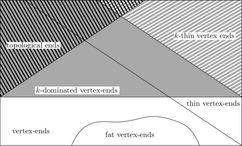
Figure 12: The classes of vertex-ends considered in this paper.

Figure 13: We put a tick in an entry of this table if the corresponding class of vertex-ends is tree-distinguishable or there is an end-faithful spanning tree for that class, respectively. If it is false we put a cross. In the one case where it is open, we put a question mark.

All positive results of Figure 13 are proved in this paper. The counterexamples corresponding to the cross in the bottom right corner were constructed by Seymour and Thomas and Thomassen as mentioned in the introduction. The other two crosses are derived from Section 3 and Section 3. The question mark in Figure 13 corresponds to the following question.

Question .

Does every graph have an end-faithful spanning tree for the thin vertex-ends?

The strengthening of Section 7 with ‘thin’ replaced by the class of vertex-ends that are dominated by finitely (or more generally: countably) many vertices is also open. Since this class contains the topological ends, this possible strengthening implies Section 2.

However, by Section 3 the class of thin vertex-ends is not tree-distinguishable. Thus, if the answer to Section 7 was ‘yes’, the obvious strategy suggested by Section 6 directly via tree-decompositions defining precisely the thin ends cannot succeed.

In the introduction of this paper we claimed that we repaired Halin’s Conjecture. In the presence of Section 7 this might deserve some further justification. Given the counterexamples against Halin’s original conjecture, we explain the subtle difference between the following two questions.

1. How can Halin’s Conjecture be repaired?

2. What is the largest possible natural subclass of the vertex-ends for which the weakening of Halin’s Conjecture is true?

The second question is still open. Candidates for that subclass are the $k$-dominated vertex-ends, or more generally the finitely or countably dominated ones. These subclasses are vertex-ends with some finiteness or countability assumption. Unlike for the topological ends, it would not have been natural to ask the weakening of Halin’s Conjecture for those subclasses in 1964. Hence these subclasses can hardly give answers to question one. The thin vertex-ends are also vertex-ends together with some finiteness assumption and might have served as a solution to question one if Diestel’s original problem was true. Since the original problem is not true (and in fact can be repaired for the topological ends), the author is convinced that Section 2 is the most natural way to repair Halin’s Conjecture.

References

- [1] Eli Berger and Henning Bruhn. Eulerian edge sets in locally finite graphs. Combinatorica, 31(1):21–38, 2011.
- [2] N. Bowler and J. Carmesin. Infinite matroids and determinacy of games. Preprint 2013, current version available at http://arxiv.org/abs/1301.5980.
- [3] H. Bruhn and M. Stein. On end degrees and infinite circuits in locally finite graphs. Combinatorica, 27:269–291, 2007.
- [4] C. Carathéodory. Über die Begrenzung einfach zusammenhängender Gebiete. Math. Ann., 73(3):323–370, 1913.
- [5] J. Carmesin. All graphs have tree-decompositions displaying their topological ends. Preprint 2015, available at http://arxiv.org/pdf/1409.6640v4.
- [6] J. Carmesin. On the end structure of infinite graphs. Preprint 2014, available at http://arxiv.org/pdf/1409.6640v1.
- [7] J. Carmesin. A short proof that every finite graph has a tree-decomposition displaying its tangles. European J. Combin., 58:61–65, 2016.
- [8] J. Carmesin. Topological cycle matroids of infinite graphs. European J. Combin, 60:135–150, 2017.
- [9] J. Carmesin, R. Diestel, M. Hamann, and F. Hundertmark. -blocks: a connectivity invariant for graphs. SIAM J. Discrete Math., 28(4):1876–1891, 2014.
- [10] J. Carmesin, R. Diestel, M. Hamann, and F. Hundertmark. Canonical tree decompositions of finite graphs I: Existence and algorithms. J. Combin. Theory (Series B), pages 1–24, 2016.
- [11] J. Carmesin, R. Diestel, F. Hundertmark, and M. Stein. Connectivity and tree-structure in finite graphs. Combinatorica, 34:11–46, 2014.
- [12] R. Diestel. Locally finite graphs with ends: a topological approach. http://arxiv.org/abs/0912.4213.
- [13] R. Diestel. The end structure of a graph: Recent results and open problems. Disc. Math., 100:313–327, 1992.
-
[14]
R. Diestel.
Graph Theory (4th edition).
Springer-Verlag, 2010.
Electronic edition available at:
http://diestel-graph-theory.com/index.html. -
[15]
R. Diestel.
Graph Theory (5th edition).
Springer-Verlag, 2016.
Electronic edition available at:
http://diestel-graph-theory.com/index.html. - [16] R. Diestel. Ends and tangles. Abhandlungen Math. Sem. Univ. Hamburg, 2017.
- [17] R. Diestel and D. Kühn. Graph-theoretical versus topological ends of graphs. J. Combin. Theory (Series B), 87:197–206, 2003.
- [18] R. Diestel and D. Kühn. On infinite cycles I. Combinatorica, 24:68–89, 2004.
- [19] R. Diestel and D. Kühn. On infinite cycles II. Combinatorica, 24:91–116, 2004.
- [20] H. Freudenthal. Über die Enden topologischer Räume und Gruppen. Math. Zeitschr., 33:692–713, 1931.
- [21] Hans Freudenthal. Über die Enden diskreter Räume und Gruppen. Comment. Math. Helv., 17:1–38, 1945.
- [22] A. Georgakopoulos. Infinite Hamilton cycles in squares of locally finite graphs. Advances in Mathematics, 220:670–705, 2009.
- [23] R. Halin. Über unendliche Wege in Graphen. Math. Annalen, 157:125–137, 1964.
- [24] R. Halin. Lattices of cuts in graphs. Abh. Math. Sem. Univ. Hamburg, 61:217–230, 1991.
- [25] M. Hamann and J. Pott. Transitivity conditions in infinite graphs. Combinatorica, 32:649–688, 2012.
- [26] B. Hughes and A. Ranicki. Ends of complexes. Cambridge Tracts in Mathematics 123, Cambridge Univ. Press, 1996.
- [27] P. Seymour and R. Thomas. An end-faithful spanning tree counterexample. Proc. Amer. Math. Soc., 113:1163–1171, 1991, no. 4.
- [28] M. Stein. Arboriticity and tree-packing in locally finite graphs. J. Combin. Theory (Series B), 96:302–312, 2006.
- [29] R. Thomas. Well-quasi-ordering infinite graphs with forbidden finite planar minor. Trans. Amer. Math. Soc., 312:279–313, 1989, no. 1.
- [30] C. Thomassen. Infinite connected graphs with no end-preserving spanning trees. J. Combin. Theory (Series B), 54:322–324, 1992.