Formation and decay of Einstein-Yang-Mills black holes

Abstract

We study various aspects of black holes and gravitational collapse in Einstein-Yang-Mills theory under the assumption of spherical symmetry. Numerical evolution on hyperboloidal surfaces extending to future null infinity is used. We begin by constructing colored and Reissner-Nordström black holes on surfaces of constant mean curvature and analyze their perturbations. These linearly perturbed black holes are then evolved into the nonlinear regime and the masses of the final Schwarzschild black holes are computed as a function of the initial horizon radius. We compare with an information-theoretic bound on the lifetime of unstable hairy black holes derived by Hod. Finally we study critical phenomena in gravitational collapse at the threshold between different Yang-Mills vacuum states of the final Schwarzschild black holes, where the $n=1$ colored black hole forms the critical solution. The work of Choptuik et al. [Phys. Rev. D 60, 124011 (1999)] is extended by using a family of initial data that includes another region in parameter space where the colored black hole with the opposite sign of the Yang-Mills potential forms the critical solution. We investigate the boundary between the two regions and discover that the Reissner-Nordström solution appears as a new approximate codimension-two attractor.

I Introduction

The Einstein-Yang-Mills equations have proven to be a particularly versatile model for studying nonlinear phenomena in gravitational collapse. Whereas for the Einstein-Maxwell equations, a version of Birkhoff’s theorem implies that any spherically symmetric solution must be static, this does not apply to Yang-Mills fields. Hence one can study interesting dynamical behavior in spherical symmetry even with modest computational resources.

What makes the Einstein-Yang-Mills equations particularly interesting is the existence of nontrivial static solutions, which play a dynamical role in gravitational collapse. The Bartnik-McKinnon solitons Bartnik and McKinnon (1988) are a discrete family of regular static solutions. There are also black hole solutions, the so-called colored black holes Bizoń (1990); Volkov and Gal’tsov (1989). They are hairy black holes in the sense that there is Yang-Mills field outside the horizon but the solutions do not carry a global charge. This is in contrast to Maxwell and Klein-Gordon fields, where black hole uniqueness theorems imply that the solutions are characterized solely by their mass, angular momentum and electric/magnetic charge evaluated at infinity Chruściel et al. (2012). The Einstein-Yang-Mills equations also admit the Reissner-Nordström black hole as an embedded Abelian solution Yasskin (1975); this solution does carry a global (magnetic) charge. We remark that although we restrict ourselves to spherical symmetry in this paper, more general axisymmetric regular and black hole solutions to the Einstein-Yang-Mills equations have been found Kleihaus and Kunz (1997a, b).

There are interesting relations between these spherically symmetric static solutions. The colored black holes have the horizon radius $R_{h}$ as a free parameter. As $R_{h}\rightarrow 0$, the solutions approach the Bartnik-McKinnon soliton. In fact, in Ashtekar et al. (2001) the authors suggested a model of the colored black hole as a bound state of a bare (Schwarzschild) black hole and the Bartnik-McKinnon soliton. And as one sends the index $n$ labeling the member of the discrete family of colored black holes to infinity, the solutions approach the Reissner-Nordström black hole.

All the above static solutions are unstable Straumann and Zhou (1990a, b); Bizoń and Wald (1991); Breitenlohner et al. (1992, 1995); Kahl (2011). Within the magnetic ansatz for the Yang-Mills field considered in this paper (Sec. II.1), the $n$th soliton and colored black hole have $n$ unstable modes Lavrelashvili and Maison (1995); Volkov et al. (1995). The Reissner-Nordström solution has an infinite number of unstable modes. This may come as a surprise because this solution is certainly stable in Einstein-Maxwell theory. An explanation in the isolated horizon framework was given in Ashtekar et al. (2001): the properly defined horizon mass in this framework is smaller than the ADM mass in Einstein-Yang-Mills theory, while the two are the same in Einstein-Maxwell theory. This mass difference in the Einstein-Yang-Mills case accounts for the available energy that can be radiated away to infinity.

The relevance of these static solutions to the Einstein-Yang-Mills equations in the context of the present paper lies in their role as critical solutions in gravitational collapse. Here one starts with a one-parameter family of regular initial data; depending on the value of the parameter, the outcome of the evolution is different. First discovered for the spherically symmetric Einstein-massless scalar field system by Choptuik Choptuik (1993), critical phenomena in gravitational collapse have since been found for a plethora of matter models coupled to the Einstein equations (see Gundlach and Martín-García (2007) for a review article). The Einstein-Yang-Mills system is particularly rich in this sense as it admits both types of critical behavior, as well as a new third type, depending on the initial data chosen. Type I and II concern the threshold between dispersal of the field to flat spacetime and black hole formation. In Type I critical collapse, black hole formation turns on at a finite mass, and the critical solution is static; in this case it is the Bartnik-McKinnon soliton Choptuik et al. (1996). In Type II critical collapse, one can make infinitesimally small black holes, and the critical solution is discretely self-similar Choptuik et al. (1996); Gundlach (1997). A new “Type III” critical phenomenon was discovered in Choptuik et al. (1999). Here the endstates on both sides of the threshold are black holes, but the Yang-Mills field is in different vacuum states. It is a curious property of the magnetic ansatz for the Yang-Mills field in spherical symmetry that there are two solutions for the connection (or vector potential), namely $w=\pm 1$, that both give rise to a vanishing field strength tensor. At the threshold between black hole formation with $w=\pm 1$, the $n=1$ colored black hole was found to be the critical solution Choptuik et al. (1999). Across the threshold there is a mass gap between the final Schwarzschild black holes.

This paper is mainly concerned with “Type III” critical collapse. We have studied this phenomenon for a wide range of parameters; in particular, we address the question how the mass gap depends on the horizon radius of the colored black hole critical solution. Motivated by work on critical collapse in the five-dimensional vacuum Einstein equations Bizoń et al. (2006), where the authors exploited discrete symmetries to find a new critical solution with two unstable modes by tuning two parameters in their initial data, we were led to the following question. The Einstein-Yang-Mills equations are invariant under a sign flip of the potential, $w\rightarrow-w$. So each colored black hole solution has a “dual” with the opposite sign. One would expect that this dual solution can also be an attractor in critical collapse, for different initial data. Is there a single smooth two-parameter family of initial data that connects both regimes? And if so, what happens at the boundary between them?

Studying these questions requires a robust and efficient numerical code that is able to carry out accurate long-term evolutions. A formulation of the Einstein equations on hyperboloidal hypersurfaces developed with Vincent Moncrief Moncrief and Rinne (2009) has proven to be extremely useful. The standard approach to numerical relativity is based on evolution on Cauchy hypersurfaces truncated at a finite distance, where boundary conditions must be imposed. The hyperboloidal approach avoids any inaccuracies resulting from imperfect boundary conditions, as the hypersurfaces extend all the way to future null infinity $\mathrsfs{I}^{+}\,$, where all the characteristics leave the computational domain and no boundary conditions need to be imposed (or they are determined uniquely by regularity considerations). In principle we obtain access to the entire future of the initial hyperboloidal surface. Furthermore, the constant mean curvature surfaces we use extend smoothly to the interior of black hole horizons so that we are able to study gravitational collapse.

In Rinne (2010) this approach was first implemented for the vacuum axisymmetric Einstein equations, achieving long-term stable evolutions of a perturbed Schwarzschild black hole. In Rinne and Moncrief (2013) we included matter sources and studied power-law tails of massless scalar and Yang-Mills fields in spherical symmetry. The present paper uses this latter implementation to study critical phenomena in gravitational collapse and associated properties of Einstein-Yang-Mills black holes.

We would like to mention a few other numerical studies (in addition to those on critical collapse mentioned above) relevant to the topic of this paper. In Pürrer and Aichelburg (2009), the authors studied power-law tails for the Einstein-Yang-Mills system. They included $\mathrsfs{I}^{+}\,$ in the computational domain by employing Bondi coordinates. Those have the disadvantage that they cannot penetrate black hole horizons, and hence are unsuitable for gravitational collapse. In Zenginoğlu (2008), tails of Yang-Mills fields were computed using hyperboloidal evolution as in our case, however on a fixed Schwarzschild background spacetime. A similar approach was used in Bizoń et al. (2010) to study interesting saddle-point behavior of Yang-Mills fields on a Schwarzschild background. The test field admits static solutions with one unstable mode, which act as unstable attractors between basins of attraction belonging to the two different vacuum states of the Yang-Mills field. This is reminiscent of the behavior seen in colored black hole critical collapse.

This paper is organized as follows. In Sec. II we briefly review our formulation of the Einstein-Yang-Mills equations and numerical method. In Sec. III we compute the relevant static solutions on the constant mean curvature surfaces we use. We also analyze their perturbations, focusing particularly on the Reissner-Nordström solution. The eigenvalues are compared with an information-theoretic bound derived by Hod Hod (2008). In Sec. IV we turn to nonlinear numerical evolutions. First we evolve linearly perturbed colored and Reissner-Nordström black holes into the nonlinear regime and investigate how their final masses depend on the initial horizon radius (Sec. IV.1). These results are useful for the following Sec. IV.2, which is devoted to critical collapse. We present an extended family of initial data that includes regions where the critical behavior found in Choptuik et al. (1999) is reproduced, as well as regions where the colored black hole with the opposite sign appears as the critical solution. We then investigate the behavior at the threshold between the two and demonstrate that the Reissner-Nordström solution is an approximate codimension-two attractor. We conclude and discuss some further questions in Sec. V.

II Formulation and methods

In this section we briefly describe the formulation of the Einstein-Yang-Mills equations and the numerical methods we use. For simplicity we restrict ourselves to spherical symmetry and a purely magnetic ansatz for the Yang-Mills field here. More details and generalizations can be found in Rinne and Moncrief (2013).

II.1 Einstein-Yang-Mills equations

The Einstein-Yang-Mills equations derive from the action

$$S=\int d^{4}x\;\mu_{\,{}^{(4)}g}\left(\frac{1}{2\kappa}\,{}^{(4)}R-\frac{1}{4}F^{(a)}_{\mu\nu}F^{(a)\mu\nu}\right),$$ (1)

where $\,{}^{(4)}g_{\mu\nu}$ is the spacetime metric, $\mu_{\,{}^{(4)}g}$ its volume element, $\kappa=8\pi$ in geometric units, $\,{}^{(4)}R$ is the scalar curvature, and $F^{(a)}_{\mu\nu}$ is the Yang-Mills field strength tensor

$$F_{\mu\nu}^{(a)}=\partial_{\mu}A_{\nu}^{(a)}-\partial_{\nu}A_{\mu}^{(a)}+\epsilon^{abc}A_{\mu}^{(b)}A_{\nu}^{(c)}.$$ (2)

(For consistency with the literature we have chosen the coupling constant $g$ in Rinne and Moncrief (2013) to be $g=1$ here.)

We write the spacetime metric as

$$\,{}^{(4)}g_{\mu\nu}=\Omega^{-2}\,{}^{(4)}\gamma_{\mu\nu},$$ (3)

where the conformal factor $\Omega\searrow 0$ at $\mathrsfs{I}^{+}\,$. In spherical symmetry we may write the conformal metric in isotropic coordinates as

$$\,{}^{(4)}\gamma=-\tilde{N}^{2}dt^{2}+(dr+rX\,dt)^{2}+r^{2}d\sigma^{2}$$ (4)

with $d\sigma^{2}=d\theta^{2}+\sin^{2}\theta\,d\phi^{2}$. We consider an ADM Arnowitt et al. (1962) decomposition with respect to the time coordinate $t$. Constant mean curvature (CMC) slicing is used; i.e., the mean curvature of the $t=\mathrm{const}$ slices is a spacetime constant $K>0$. The tracefree part of the ADM momentum $\pi^{\mathrm{tr}\,ij}$ has only one degree of freedom in spherical symmetry, which we take to be $\pi:=(r^{4}\sin\theta)^{-1}\pi^{\mathrm{tr}\,rr}$. The gravitational field is thus described by the four variables $\Omega,\tilde{N},X$ and $\pi$, which are functions of $t$ and $r$ only. In the following we use an overdot to denote $t$-derivatives and a prime to denote $r$-derivatives.

Preserving the isotropic spatial coordinate condition and the CMC slicing condition under the time evolution yields

$$0 = r^{-1}X^{\prime}+\textstyle\frac{3}{2}\tilde{N}\pi,$$ (5)

$$0 = -\Omega^{2}\tilde{N}^{\prime\prime}+3\Omega\Omega^{\prime}\tilde{N}^{\prime}-2\Omega^{2}r^{-1}\tilde{N}^{\prime}-\textstyle\frac{3}{2}\Omega^{\prime 2}\tilde{N}$$ (6)

$$+{\textstyle\frac{1}{6}}\tilde{N}K^{2}+\textstyle\frac{15}{8}\tilde{N}\Omega^{2}r^{4}\pi^{2}+{\textstyle\frac{1}{2}}\kappa\tilde{N}\Omega^{4}(\tilde{S}+2\tilde{\rho}).$$

The Einstein equations reduce to the Hamiltonian and momentum constraint,

$$0 = -4\Omega\Omega^{\prime\prime}+6\Omega^{\prime 2}-8\Omega r^{-1}\Omega^{\prime}+\textstyle\frac{3}{2}\Omega^{2}r^{4}\pi^{2}$$ (7)

$$-\textstyle\frac{2}{3}K^{2}+2\kappa\Omega^{4}\tilde{\rho},$$

$$0 = \Omega(r\pi^{\prime}+5\pi)-2r\Omega^{\prime}\pi+\kappa\Omega^{3}r^{-1}\tilde{J}^{r}.$$ (8)

The source terms $\tilde{\rho}$, $\tilde{S}$ and $\tilde{J}^{r}$ in (6)–(8) are components of the conformally rescaled energy-momentum tensor $\tilde{T}_{\mu\nu}=\Omega^{-2}T_{\mu\nu}$ and are defined for Yang-Mills fields below in (15) and (16).

The Yang-Mills equations are conformally invariant and hence we may define the fields in terms of the conformal metric $\,{}^{(4)}\gamma_{\mu\nu}$, indicated by tildes in the following. We take the gauge group to be SU(2) and adopt a purely magnetic ansatz for the vector potential in temporal gauge,

$$\tilde{A}^{i(a)}=[aij]x^{j}W(t,r),\quad\tilde{A}_{0}^{(a)}=0,$$ (9)

where the symbol $[aij]$ is totally antisymmetric with $[123]=1$. (We considered a more general ansatz in Rinne and Moncrief (2013).) In the literature Bizoń (1990); Straumann and Zhou (1990b); Choptuik et al. (1996, 1999) the vector potential is often written in “(maximally) Abelian gauge” Bartnik (1997) as

$$\tilde{A}=w\tau^{\theta}d\theta+(\cot\theta\,\tau^{r}+w\tau^{\phi})\sin\theta\,d\phi$$ (10)

where $\tau^{a}$ are the Pauli matrices. The two potentials $W$ and $w$ in (9) and (10) are related by

$$\qquad W=\frac{1-w}{r^{2}}.$$ (11)

We prefer to use $W$ also for numerical reasons (regularity at $r=0$). The electric field is defined as

$$\tilde{\mathcal{D}}^{i(a)}=\mu_{\,{}^{(4)}\gamma}\,\tilde{F}^{(a)0i}=[aij]x^{j}D(t,r).$$ (12)

The Yang-Mills field equations take the form of a nonlinear wave equation for $W$:

$$\dot{W} = rXW^{\prime}+2XW-\tilde{N}D,$$ (13)

$$\dot{D} = (rXD-\tilde{N}W^{\prime})^{\prime}+2XD-4\tilde{N}r^{-1}W^{\prime}$$ (14)

$$-2Wr^{-1}\tilde{N}^{\prime}+\tilde{N}W^{2}(r^{2}W-3).$$

The matter source terms in (6)–(8) are given by

$$\tilde{\rho}=\tilde{S} = {\textstyle\frac{1}{2}}\big{[}2r^{2}D^{2}+12W^{2}+r^{2}W^{3}(r^{2}W-4)$$ (15)

$$\quad+2rW^{\prime}(rW^{\prime}+4W)\big{]},$$

$$\tilde{J}^{r} = 2rD(rW^{\prime}+2W).$$ (16)

II.2 Numerical methods

We discretize the equations in space using fourth-order finite differences. A mapping of the radial coordinate with an adjustable parameter Rinne and Moncrief (2013) is used in order to provide more resolution where it is needed, especially near the black hole horizon where the fields typically develop steep gradients. The outermost grid point is placed at $\mathrsfs{I}^{+}\,$, which we choose to correspond to $r=1$. Typical resolutions used for the simulations in this paper range from $500$ to $2000$ radial grid points.

Following the method of lines, the evolution equations (13) and (14) are first discretized in space and then integrated forward in time using a fourth-order Runge-Kutta method with sixth-order Kreiss-Oliger dissipation Kreiss and Oliger (1973). At each time step, the ODEs (5)–(8) are solved using a Newton-Raphson method, at each iteration solving the resulting linear system using a direct band-diagonal solver.

Boundary conditions at the origin $r=0$ (before a black hole forms) follow from the fact that all the fields $\Omega,\tilde{N},X,\pi,W,D$ are even functions of $r$. Once an apparent horizon forms, we place an excision boundary sufficiently far inside it and remove its interior from the computational domain. One-sided finite differences are used at this inner boundary. Since the excision boundary lies inside the black hole, all characteristics leave the domain and hence no boundary conditions are required for the evolution equations (13) and (14). The outer boundary $\mathrsfs{I}^{+}\,$ is an outflow boundary as well and is treated in the same fashion. Boundary conditions for the elliptic equations (5)–(8) follow from regularity at $\mathrsfs{I}^{+}\,$ and compatibility with the remaining Einstein evolution equations at the excision boundary; see Rinne and Moncrief (2013) for details.

In all our evolutions the value of the mean curvature is taken to be $K=1/2$.

The code has been written in and the figures produced with Python, making use of the NumPy, SciPy and matplotlib extensions (for an excellent recent introduction see Stewart (2014)).

III Static solutions and their linear perturbations

In order to evolve perturbed Yang-Mills black holes and to analyze their role in dynamical collapse evolutions, we need first to construct these solutions. So far these solutions have been considered on maximal slices $K=0$ approaching spacelike infinity (Sec. III.1), whereas we use CMC slices $K>0$ approaching future null infinity. We develop a general procedure for transforming a static solution on a maximal slice to a CMC slice in Sec. III.2. Finally we find the unstable eigenmodes of the solutions in Sec. III.3.

III.1 Solutions on a maximal slice

Static spherically symmetric solutions to the Einstein-Yang-Mills equations are most commonly constructed in polar-areal coordinates, in which the spacetime metric takes the form

$$\,{}^{(4)}g = -\left(1-\frac{2m}{R}\right)e^{-2\delta}dT^{2}+\left(1-\frac{2m}{R}\right)^{-1}dR^{2}$$ (17)

$$+R^{2}d\sigma^{2},$$

where $m$ and $\delta$ are functions of the areal radius $R$ only.

An example in closed form is the familiar Schwarzschild solution, a vacuum solution to the Einstein equations with

$$m=M=\mathrm{const},\quad\delta=0,\quad w=\pm 1,\quad D=0,$$ (18)

$M$ being the black hole mass, $M=0$ corresponding to Minkowski spacetime. Note there are two different solutions for the Yang-Mills potential, $w=\pm 1$, that both give rise to vacuum $\tilde{F}^{(a)}_{\mu\nu}=0$. This plays a crucial role in critical collapse where the end state can be a Schwarzschild black hole with the Yang-Mills field in either of its two vacua.

Another closed-form static solution to the Einstein-Yang-Mills equations relevant to the present paper is the Reissner-Nordström solution Yasskin (1975) (with unit magnetic charge)

$$m=M-\frac{1}{2R},\quad\delta=0,\quad w=0,\quad D=0.$$ (19)

Further spherically symmetric, static, purely magnetic solutions to the Einstein-Yang-Mills equations have been found: a discrete family of regular solutions known as Bartnik-McKinnon solitons Bartnik and McKinnon (1988) and a discrete family of colored black holes Bizoń (1990); Volkov and Gal’tsov (1989). These solutions are not known in closed form but can be constructed numerically by solving the static Einstein-Yang-Mills equations, which read

$$0 = R^{2}\left(1-\frac{2m}{R}\right)w_{,RR}$$ (20)

$$+\left[2m-\frac{(1-w^{2})^{2}}{R}\right]w_{,R}+(1-w^{2})w,$$

$$m_{,R} = \left(1-\frac{2m}{R}\right)\left(w_{,R}\right)^{2}+\frac{(1-w^{2})^{2}}{2R^{2}},$$ (21)

$$\delta_{,R} = -\frac{2}{R}(w_{,R})^{2}.$$ (22)

We proceed as in Bizoń (1990). Expanding the solution about the black hole event horizon at $R=R_{h}$, where $R_{h}=2m(R_{h})$, one finds that given a value of $R_{h}$, there is one undetermined parameter at the horizon, namely $b:=w(R_{h})$. We integrate the pair of ODEs (20) and (21) numerically from the horizon to some large value of $R$ and, using the shooting method, search for a value of $b>0$ such that $w\rightarrow-1$ as $R\rightarrow\infty$. Here we are only interested in the solution with one zero of $w$, the $n=1$ colored black hole. Once the solution for $w$ and $m$ is found, (22) is solved for $\delta$. We choose the initial value of $\delta$ at the horizon to be $\delta_{h}=0$; later a constant is subtracted so that $\delta\rightarrow 0$ as $R\rightarrow\infty$, ensuring that the metric (17) approaches the flat metric in the standard coordinates as $R\rightarrow\infty$.

Note that because (20)–(22) are invariant under $w\rightarrow-w$, each static solution has a related solution with the opposite sign of $w$. This will play an important role in Sec. IV.2.

III.2 Transforming to a CMC slice

Given the metric (17) on the maximal slice, we now show how to transform it to a CMC slice and a conformally compactified radial coordinate. This generalizes the method used in Malec and Ó Murchadha (2003) to find the Schwarzschild solution on CMC slices to arbitrary static spherically symmetric spacetimes.

First we introduce a new time coordinate

$$t=T-h(R),$$ (23)

where $h(R)$ is the height function. The mean curvature of a $t=\mathrm{const}$ slice is found to be

$$K=e^{\delta}R^{-2}\frac{d}{dR}\left\{\frac{R^{2}e^{-\delta}h_{,R}\left(1-\frac{2m}{R}\right)}{\left[\left(1-\frac{2m}{R}\right)^{-1}e^{2\delta}-(h_{,R})^{2}\left(1-\frac{2m}{R}\right)\right]^{1/2}}\right\}.$$ (24)

We require this to be a constant $K>0$. Let us introduce the function

$$\Delta(R):=\frac{3}{R^{3}}\left(\int_{R_{h}}^{R}\bar{R}^{2}e^{-\delta(\bar{R})}d\bar{R}+C_{h}\right),$$ (25)

where $C_{h}$ is an integration constant discussed below, and $R_{h}$ is the areal radius of the horizon. Eq. (24) can now be solved for $h_{,R}$ to obtain

$$h_{,R}=\frac{{\textstyle\frac{1}{3}}K\Delta e^{2\delta}}{\left(1-\frac{2m}{R}\right)f},$$ (26)

where we have defined

$$f:=\left[\frac{1}{R^{2}}\left(1-\frac{2m}{R}\right)+e^{2\delta}\left({\textstyle\frac{1}{3}}K\Delta\right)^{2}\right]^{1/2}.$$ (27)

Using (26) we can write the metric with respect to the new $t$ coordinate as

$$\,{}^{(4)}g=-N^{2}dt^{2}+\,{}^{(3)}g_{RR}(dR+N^{R}dt)^{2}+R^{2}d\sigma^{2},$$ (28)

where

$$N=e^{-\delta}Rf,\quad N^{R}=-{\textstyle\frac{1}{3}}K\Delta R^{2}f,\quad\,{}^{(3)}g_{RR}=(Rf)^{-2}.$$ (29)

Next we transform to conformal radius $r$ defined by

$$\frac{dr}{dR}=\frac{r[\,{}^{(3)}g_{RR}]^{1/2}}{R}=\frac{r}{R^{2}f}.$$ (30)

Thus we arrive at the line element (3)–(4) with

$$\Omega=\frac{r}{R},\quad\tilde{N}=re^{-\delta}f,\quad X=-{\textstyle\frac{1}{3}}K\Delta.$$ (31)

We also compute

$$\pi=\textstyle\frac{2}{3}KRr^{-3}(1-e^{\delta}\Delta),$$ (32)

and from $\dot{W}=0$ in (13) we find the electric field

$$D={\textstyle\frac{1}{3}}K\Delta e^{\delta}r^{-3}R^{2}w_{,R}.$$ (33)

This completes the computation of all the evolved fields.

Numerically, we need to integrate (25) and (30) to find $\Delta(R)$ and $r(R)$. The conformal radius $r$ may be multiplied by an overall constant so that $r=1$ at $R=\infty$ corresponding to $\mathrsfs{I}^{+}\,$. The function $r(R)$ is inverted (by interpolation) to find $R(r)$ on the numerical grid chosen for the conformal radius $r$, and this then allows us to specify all the fields as functions of $r$ on the numerical grid.

Finally we comment on the integration constant $C_{h}$ in (25). The expansion of the outgoing radial null rays is computed as

$$\Theta_{+}={\textstyle\frac{1}{3}}K\Delta e^{\delta}+f.$$ (34)

At the horizon, we have $R_{h}=2m_{h}$ and thus

$$\Theta_{+,h}={\textstyle\frac{1}{3}}Ke^{\delta_{h}}(\Delta_{h}+|\Delta_{h}|).$$ (35)

Hence in order to have $\Theta_{+,h}=0$ we need the constant $C_{h}<0$ in (25). In Schwarzschild (and also Reissner-Nordström) spacetime we have $\delta\equiv 0$, and the constant $C$ appearing in the metric on the CMC slice in Malec and Ó Murchadha (2003) is related to our constant $C_{h}$ via

$$C_{h}=-\frac{C}{K}+\frac{1}{3}R_{h}^{3}.$$ (36)

III.3 Mode analysis

In order to compute the eigenmodes of linear perturbations about static solutions of the Einstein-Yang-Mills equations, we prefer to work on the CMC slice using conformal radius. This is because our coordinates smoothly extend to the black hole interior, unlike the standard Schwarzschild-like coordinates, or Kruskal-Szekeres coordinates where the horizon is pushed off to negative infinity in the radial coordinate used (cf. the debate on smoothness of the modes in Straumann and Zhou (1990b); Bizoń (1991); Bizoń and Wald (1991)). Also our computational domain extends all the way out to future null infinity.

Separating the time dependence, we make the general ansatz

$$w=\bar{w}+e^{\lambda t}\delta w(r),$$ (37)

with $\lambda\in\mathbb{C}$, where $\bar{w}$ refers to the static background solution and $\delta w$ to its linear perturbation. We are looking for unstable modes corresponding to positive real eigenvalues $\lambda>0$. Substituting the ansatz (37) into the dynamical Einstein-Yang-Mills equations (Sec. II.1), we find the pulsation equation

$$c_{2}\delta w^{\prime\prime}+c_{1}\delta w^{\prime}+c_{0}\delta w=0,$$ (38)

where as in Sec. II.1 a prime refers to a derivative with respect to conformal radius $r$. The coefficients $c_{i}$ are given by

$$c_{2} = \tilde{N}^{2}-r^{2}X^{2},$$ (39)

$$c_{1} = \tilde{N}^{-1}\tilde{N}^{\prime}(\tilde{N}^{2}+r^{2}X^{2})-2r^{2}XX^{\prime}-2rX^{2}$$ (40)

$$+2\lambda rX,$$

$$c_{0} = -2r^{-2}\tilde{N}^{2}+3\tilde{N}^{2}r^{-2}(1-\bar{w}^{2})$$ (41)

$$+\lambda(X-\tilde{N}^{-1}\tilde{N}^{\prime}rX+rX^{\prime})-\lambda^{2},$$

where $\tilde{N}$ and $X$ are to be evaluated for the background solution. At $\mathrsfs{I}^{+}\,$ the following conditions hold Rinne and Moncrief (2013):

$$r\tilde{N}^{\prime}=\tilde{N},\quad rX=-\tilde{N},\quad X^{\prime}=0.$$ (42)

Substituting these into (38) yields

$$\delta w^{\prime}=-\delta w\,\frac{\hat{\lambda}^{2}+2r^{-2}}{2\hat{\lambda}}$$ (43)

at $\mathrsfs{I}^{+}\,$, where we have defined $\hat{\lambda}:=\lambda/\tilde{N}_{\infty}$, and we choose the lapse at $\mathrsfs{I}^{+}\,$ to be $\tilde{N}_{\infty}=K/3$ so that time $t$ agrees with the standard time coordinate in flat spacetime asymptotically Rinne and Moncrief (2013). The value of $\delta w$ at $\mathrsfs{I}^{+}\,$ can be freely chosen, and (43) provides us with initial data for the pulsation equation (38) at $\mathrsfs{I}^{+}\,$, which we integrate inwards toward the horizon. There the solution $\delta w$ must be finite, and this condition determines the eigenvalues $\lambda$. Once an eigenvalue has been found, (38) can be integrated to the interior of the horizon as well.

For the $n=1$ colored black hole, there is precisely one unstable mode, which was first computed in Straumann and Zhou (1990b). A plot of the eigenvalue as a function of the horizon radius can be found in Bizoń and Chmaj (2000). Our results are in good agreement with this.

In the Einstein-Yang-Mills system, the Reissner-Nordström solution has an infinite number of unstable modes Bizoń and Wald (1991); Breitenlohner et al. (1995); Kahl (2011). The $n$th mode has $n$ zeros, $n=0,1,2,\ldots$ The first three modes are plotted in Fig. 1 for one value of the horizon radius. Note how they are perfectly smooth at the horizon in our coordinates. Fig. 2 shows the corresponding eigenvalues as functions of horizon radius.

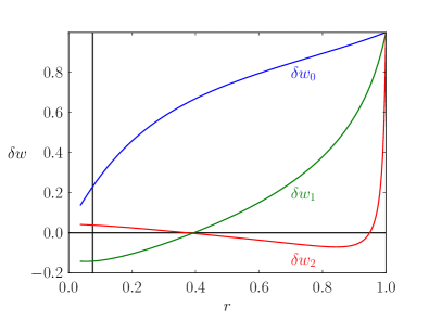
Figure 1: The first three unstable eigenmodes of the Reissner-Nordström solution as a function of conformal radius $r$. The horizon radius $R_{h}=2.57$ and slicing constant $C_{h}=-1.84$ in (25) have been chosen to agree with the attractor observed in the evolutions of Sec. IV.2. The modes have been normalized so that $\delta w=1$ at $\mathrsfs{I}^{+}\,$. The location of the horizon is indicated by the vertical line.

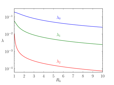
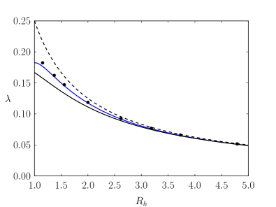
Figure 2: Top: the first three unstable eigenvalues of the Reissner-Nordström solution as functions of horizon radius $R_{h}$. Bottom: comparison of the dominant eigenvalue (middle curve, solid blue) with Hod’s bound Hod (2008) in its weak (upper curve, dashed black) and strong (lower curve, solid black) form, where for the latter we take $\Delta\mathcal{E}$ to be the entire mass outside the horizon. If instead $\Delta\mathcal{E}$ is taken to be the fraction of this mass that falls into the black hole in a nonlinear evolution, the black points result.

It is interesting to compare the eigenvalues of the Reissner-Nordström solution with a bound on the lifetime of unstable hairy black holes proposed by Hod Hod (2008), based on arguments from quantum information theory. This bound was shown in Hod (2008) to be satisfied for the $n=1$ colored black hole but the situation for the Reissner-Nordström solution remained inconclusive. The bound implies that the eigenvalues should be bounded by

$$\lambda\leqslant[4(R_{h}+\Delta\mathcal{E})]^{-1}\leqslant(4R_{h})^{-1}.$$ (44)

We refer to the first bound on the right-hand side as the strong bound and the second as the weak bound. In the strong bound, $\Delta\mathcal{E}$ is the mass that is swallowed by the unstable black hole in a nonlinear evolution. As a first approximation, this was taken in Hod (2008) to be the entire mass outside the horizon of the initial black hole, $\Delta\mathcal{E}=\Delta M_{\mathrm{max}}=M-{\textstyle\frac{1}{2}}R_{h}$. For the Reissner-Nordström solution, we have

$$M=\frac{R_{h}^{2}+1}{2R_{h}}\,\Rightarrow\,\Delta M_{\mathrm{max}}=M-\frac{R_{h}}{2}=\frac{1}{2R_{h}}.$$ (45)

Figure 2 shows that close to the extremal value $R_{h}=1$, only the weak bound is satisfied, whereas the above version of the strong bound is violated (unlike for the colored black holes, where both are satisfied Hod (2008)). However, $\Delta\mathcal{E}$ should really be taken to be the actual amount of hair that falls into the black hole; this will be computed in the following section.

IV Nonlinear evolutions

In this section we perform nonlinear numerical evolutions of the Einstein-Yang-Mills equations. While we are ultimately interested in the formation (and later decay) of Yang-Mills black holes as intermediate attractors in gravitational collapse (Sec. IV.2), we begin by studying the final fate of linear perturbations of these static solutions (Sec. IV.1). The reason is that in critical collapse, the situation near the critical solution can be described in terms of linear perturbations. As we shall see, the critical solutions relevant to the present study are the $n=1$ colored black holes and the Reissner-Nordström solution. In order to approach these critical solutions, one needs to tune one (or even two, as in Sec. IV.2) parameters in the initial data, which is done by a bisection search involving a large number of evolutions. If we are only interested in the behavior after the critical solution is approached, it suffices and is much less time-consuming to start with the linearly perturbed critical solution and evolve it into the nonlinear regime.

IV.1 Perturbed black holes

We begin with a colored black hole solution of a given horizon radius $R_{h0}$ and add to it the unstable mode with a typical amplitude $\sim 5\times 10^{-3}$. Depending on the sign of the perturbation, the solution evolves to a Schwarzschild black hole with the Yang-Mills field either in its $w=+1$ or $w=-1$ vacuum state. Fig. 3 illustrates that in a $w\rightarrow+1$ evolution, most (but not all) of the Yang-Mills hair falls into the black hole, whereas in a $w\rightarrow-1$ evolution, most (but not all) of it escapes to infinity. The resulting mass gap is plotted in Fig. 4 as a function of the horizon radius of the initial colored black hole for a few evolutions. Note that the case $R_{h}=0$ corresponds to the regular, horizon-less Bartnik-McKinnon soliton, which either disperses to Minkowski spacetime or collapses to a Schwarzschild black hole swallowing nearly all of the soliton’s mass.

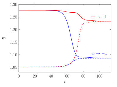
Figure 3: Bondi mass $m_{\mathrsfs{I}^{+}\,}$ (solid lines) and apparent horizon mass $m_{h}={\textstyle\frac{1}{2}}R_{h}$ (dashed lines) as functions of time for two perturbed colored black hole evolutions with opposite sign of the perturbation, leading to final vacuum states $w=-1$ (blue) or $w=+1$ (red). The initial horizon radius is $R_{h}=2.11$ (chosen to agree with the attractor of the evolution with $r_{b}=0.7$ in Sec. IV.2).

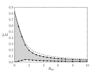
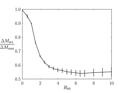
Figure 4: Masses of colored black holes and their decay products. In the top panel, the dashed line shows the total mass of hair $\Delta M_{\mathrm{max}}=M-{\textstyle\frac{1}{2}}R_{h0}$ outside the horizon radius $R_{h0}$ of the initial colored black hole. The upper solid line represents the quantity $M_{f+}-{\textstyle\frac{1}{2}}R_{h0}$, where $M_{f+}$ is the mass of the final Schwarzschild black hole in a $w\rightarrow+1$ evolution. The lower solid line shows the corresponding $M_{f-}-{\textstyle\frac{1}{2}}R_{h}$ for a $w\rightarrow-1$ evolution. The difference $\Delta M_{\mathrm{act}}=M_{f+}-M_{f-}$ is the actual mass gap, indicated by the shaded region. The ratio of the actual and the maximal mass gap is plotted in the lower panel. The error bars indicate an estimate of the numerical accuracy.

In Fig. 4 we compare the actual mass gap observed in the nonlinear evolutions with the maximal mass gap (see Fig. 2 of Bizoń and Chmaj (2000)) that would result if either all of the Yang-Mills hair outside the horizon fell into the black hole or all of it escaped to infinity. In Bizoń and Chmaj (2000) the authors wondered whether the actual mass gap goes to zero at some large but finite $R_{h}$, so that the line of colored black holes in a phase space diagram Choptuik et al. (1999) would terminate at a finite distance, “in an amusing similarity to the gas-liquid boundary on phase diagrams for typical substances”. While our results cannot exclude this possibility, if the trend continues then the mass gap will only approach zero asymptotically as $R_{h}\rightarrow\infty$. We remark that the numerical evolution is stopped when the horizon mass ${\textstyle\frac{1}{2}}R_{h}$ and the Bondi mass differ by less than one part in $10^{4}$, so we can only determine the final mass up to that accuracy. As a result, the relative mass gap, being the quotient of two small quantities, has relatively large errors for large values of $R_{h}$.

We repeat this calculation for the Reissner-Nordström solution in Fig. 5, where we add the dominant unstable mode. Since the background solution has $w=0$ and the Einstein-Yang-Mills equations are symmetric under $w\rightarrow-w$, the evolutions for both signs of the perturbation are identical up to a sign, and there is no mass gap. We have already computed the mass outside the horizon of the Reissner-Nordström solution, $\Delta M_{\mathrm{max}}$ in (45). The part of this mass that falls into the black hole in a nonlinear evolution is shown in Fig. 5. It shows remarkably little variation, starting at about $50\%$ of $\Delta M_{\mathrm{max}}$ for $R_{h0}\rightarrow 1$ and settling down to about $40\%$ for $R\sim 10$. Since we cannot evolve the extremal Reissner-Nordström solution ($R_{h}=1$) using our current numerical implementation, we only consider horizon radii close to but larger than this limit.

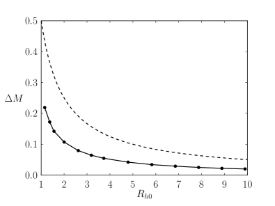
Figure 5: Masses of Reissner-Nordström black holes and their decay products. The dashed line shows the mass of the Yang-Mills field outside the horizon radius $R_{h0}$ of the initial Reissner-Nordström black hole, $\Delta M_{\mathrm{max}}=M-{\textstyle\frac{1}{2}}R_{h0}$. The solid line represents the quantity $M_{f}-{\textstyle\frac{1}{2}}R_{h0}$, where $M_{f}$ is the mass of the final Schwarzschild black hole.

With these results we now return to the comparison of the dominant unstable eigenvalue of the Reissner-Nordström solution with the bound derived by Hod Hod (2008), the lower panel of Fig. 2. If we take $\Delta\mathcal{E}$ in (44) to be the actual amount of mass that falls into the black hole during the evolution, $\Delta\mathcal{E}=M_{f}-{\textstyle\frac{1}{2}}R_{h0}$, then the strong version of the bound is satisfied and saturated remarkably closely.

IV.2 Critical collapse

In this section we study the formation of black holes from regular initial data. The family of initial data for the Yang-Mills potential $w$ we consider consists of a kink as in Choptuik et al. (1999) with an additional Gaussian bump:

$$w(0,r)=-\tanh\left(\frac{r-r_{k}}{\sigma_{k}}\right)-A_{b}\exp\left[-\frac{(r-r_{b})^{2}}{2\sigma_{b}^{2}}\right].$$ (46)

From this we form our evolved field $W$, rolling it off with an additional Gaussian to ensure regularity at $r=0$:

$$W(0,r)=\frac{1-w(0,r)}{r^{2}}\left[1-\exp\left(-\frac{r^{2}}{2\sigma_{r}^{2}}\right)\right].$$ (47)

The time derivative of $w$ is taken to vanish initially. The constraint equations are solved for the gravitational field.

In Choptuik et al. (1999) colored black hole critical collapse was observed in the kink family of initial data (without our additional Gaussian, $A_{b}=0$ in (46)). We observe the same phenomenon in regions of our extended family. Since the Einstein-Yang-Mills equations are symmetric under $w\rightarrow-w$, it is tempting to search for regions in parameter space where the critical solution is the one with the opposite sign as in the original simulations of Choptuik et al. (1999). Indeed such regions exist, and an extensive search in parameter space led us to discover a two-parameter family that smoothly connects two regions with opposite signs of the colored black hole critical solution. We fix $\sigma_{k}=\sigma_{b}=\sigma_{r}=0.05$ and $r_{k}=0.4$ in (46) and vary the two parameters $r_{b}$ and $A_{b}$.

For various values of $r_{b}$, we perform a bisection search for $A_{b}$ between the two possible outcomes of the evolution, Schwarzschild black holes with $w=\pm 1$ (Fig. 6). Let us call the solution that is thus approached $A_{b}$-critical. For values of $r_{b}$ well smaller than some critical value $r_{b}^{*}\approx 0.6036$, we find that the critical solution is a colored black hole with $w=-1$ at $\mathrsfs{I}^{+}\,$, as in Choptuik et al. (1999). For $r_{b}>r_{b}^{*}$, the colored black hole with the opposite sign of $w$ is approached (Fig. 7).

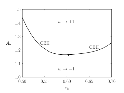
Figure 6: The critical line in the two-dimensional parameter space. For values of $A_{b}$ above (below) the threshold, the evolution ultimately approaches a Schwarzschild black hole with $w\equiv+1$ ($-1$). The critical value $r_{b}=r_{b}^{*}$ is indicated by a dot. For $r_{b}<r_{b}^{*}$ ($r_{b}>r_{b}^{*}$), the critical solution is a colored black hole (CBH) with $w=-1$ ($w=+1$) at $\mathrsfs{I}^{+}\,$.

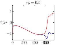
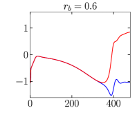
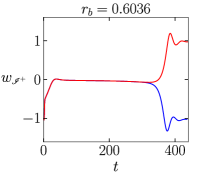
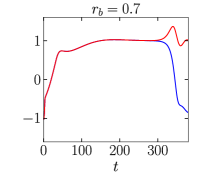
Figure 7: $A_{b}$-near-critical evolutions of $w$ at future null infinity for a few typical values of $r_{b}$. The value of $A_{b}$ for the slightly supercritical (upper curves, red) and slightly subcritical (lower curves, blue) evolutions differs by $\approx 10^{-14}$.

The behavior we find at the $A_{b}$-critical threshold is the same as reported in Choptuik et al. (1999). Figure 8 shows $w$ at $\mathrsfs{I}^{+}\,$ as a function of time for a slightly $A_{b}$-supercritical evolution with $r_{b}=0.7$. The black hole forms at $t=28$, and the different phases of the evolution are clearly visible: approach to the colored black hole with $w=+1$ at $\mathrsfs{I}^{+}\,$, exponential instability of this intermediate attractor, and ringdown to the final Schwarzschild black hole with $w=+1$ at $\mathrsfs{I}^{+}\,$. We only plot $w$ at $\mathrsfs{I}^{+}\,$ here, however the approach to the static solutions can be observed at all radii.

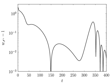
Figure 8: An ever so slightly $A_{b}$-supercritical evolution of $w$ at $\mathrsfs{I}^{+}\,$ for $r_{b}=0.7$.

The time $t=\tau$ when the evolution departs from the critical solution is plotted for this $r_{b}=0.7$ evolution as the dashed line in Fig. 9. Here we define $\tau$ as the time when the zero of $w$ crosses $r=0.5$ in slightly subcritical evolutions. It exhibits critical scaling as in Type I critical collapse Gundlach and Martín-García (2007),

$$\tau=\mathrm{const}-\gamma\ln|A_{b}-A_{b}^{*}|$$ (48)

with a fitted value $\gamma=9.79$. Using the methods of Sec. III.3 we compute the eigenvalue of the unstable mode of the colored black hole (with $R_{h}=2.11$ for this evolution) as $\lambda=0.1020$. Hence $1/\lambda=9.80\approx\gamma$, as expected. Our results demonstrate the universality of the critical phenomenon discovered in Choptuik et al. (1999), as the family of initial data and the critical parameter we use is different (recall the Gaussian in (46) was not included in Choptuik et al. (1999)).

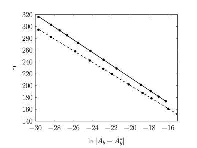
Figure 9: The time $t=\tau$ when the evolution departs from the critical solution as a function of the logarithm of the parameter distance in $A_{b}$-critical searches. The dashed line is for $r_{b}=0.7$, where the critical solution is a colored black hole, whereas the solid line is for $r_{b}=0.6036\approx r_{b}^{*}$, where the critical solution is the Reissner-Nordström black hole. The lines are linear fits to the data points.

We also observe a mass gap between the slightly $A_{b}$-subcritical and slightly $A_{b}$-supercritical evolutions, and this agrees well with the mass gap we obtained in Sec. IV.1 by starting off with the perturbed colored black hole directly. (For the case $R_{h}=2.11$ considered above, the mass gap between near-critical evolutions is found to be $\Delta M=0.1465$; the mass gap from the perturbed colored black hole evolutions is $\Delta M=0.1469$.)

The question arises what happens as $r_{b}$ approaches the critical value $r_{b}^{*}$ that separates the two regions of colored black hole critical behavior with opposite signs of the critical solution. We find that as we tune $r_{b}$ closer and closer to the threshold, the Reissner-Nordström solution corresponding to $w=0$ appears as a new approximate unstable attractor before the colored black hole is approached (Fig. 7); the term approximate will be explained below. Very close to $r_{b}^{*}$ this new attractor dominates and the colored black hole attractor is no longer visible. (Seeing it would require an excessive amount of fine-tuning of $A_{b}$.)

We now analyze the behavior at the $r_{b}$-critical threshold in more detail. First we look at the time the solution spends near the Reissner-Nordström attractor in an $A_{b}$-critical search (the solid line in Fig. 9), this time with $r_{b}\approx r_{b}^{*}$. Here we define $\tau$ as the time when $w$ first passes the value $w=0.1$ at $\mathrsfs{I}^{+}\,$ in slightly $A_{b}$-supercritical evolutions. Again this shows critical scaling, with a fitted exponent $\gamma=10.67$. This agrees well with the inverse of the dominant eigenvalue of the Reissner-Nordström attractor (which has horizon radius $R_{h}=2.57$): $\lambda_{0}=0.09348\,\Rightarrow\,1/\lambda_{0}=10.70$.

Next we look at the departure time from the Reissner-Nordström attractor (defined as above) tangential to the critical line, i.e. we tune $A_{b}$ very closely to threshold and vary $r_{b}$. The result is shown in Fig. 10. Critical scaling with a fitted exponent $\gamma=93.3$ is found, which differs by about one order of magnitude from the exponent away from the critical line. This value agrees well with the next-to-dominant eigenvalue of the Reissner-Nordström solution, $\lambda_{1}=0.01062\,\Rightarrow\,1/\lambda_{1}=94.2$.

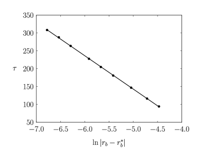
Figure 10: The time $t=\tau$ when the evolution departs from the Reissner-Nordström attractor as a function of $r_{b}$ along the critical line, where $A_{b}$ has been tuned very closely to threshold. The line is a linear fit to the data points.

Finally we evaluate the mass gap $\Delta M=M_{f+}-M_{f-}$ between slightly $A_{b}$-subcritical and $A_{b}$-supercritical evolutions as a function of $r_{b}$ (Fig. 11). This vanishes linearly as $r_{b}\rightarrow r_{b}^{*}$, consistent with perturbations about Reissner-Nordström spacetime, which have vanishing mass gap (Sec. IV.1). In fact, the zero of the mass gap allows for the most accurate determination of the critical value $r_{b}^{*}$.

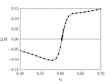
Figure 11: The mass gap $\Delta M=M_{f+}-M_{f-}$ across the $A_{b}$-critical threshold as a function of $r_{b}$.

All these results are consistent with the picture (Fig. 6) that the codimension-two unstable attractor that divides the critical line in the two-dimensional parameter space into colored black hole solutions with opposite sign is the Reissner-Nordström solution. Along its dominant unstable mode, the solution departs immediately to one of the final Schwarzschild endstates. Along its second unstable mode, it first approaches one of the copies of the $n=1$ colored black hole (with either sign) before departing to Schwarzschild.

There remains a puzzle though: the Reissner-Nordström solution has an infinite number of unstable modes. By tuning two parameters in the initial data, one can eliminate the two dominant modes but in general not any of the other unstable modes. These modes have an increasing number of radial oscillations. When decomposing the near-critical solution into the eigenmodes, the coefficients must therefore fall off fast with the mode number, as the solution certainly remains smooth. Thus we would expect the near-critical solution to look qualitatively like the third unstable mode, which has two zeros. Indeed this is what we see (Fig. 12). The third eigenvalue is much smaller than the second (by a factor $33$) and hence the associated eigenmode is seen as almost constant in time.

The Reissner-Nordström solution is thus only an approximate codimension-two attractor, but one that is approached remarkably closely.

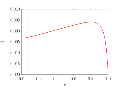
Figure 12: The Yang-Mills potential $w$ as a function of conformal radius $r$ at time $t=250$ for an evolution with $r_{b}=0.6036\approx r_{b}^{*}$. Compare with $\delta w_{2}$ in Fig. 1.

V Conclusions and discussion

We investigated static spherically symmetric black hole solutions to the Einstein-Yang-Mills equations, in particular the $n=1$ colored black hole and the magnetic Reissner-Nordström solution, and the role they play in gravitational collapse.

A new formulation and numerical implementation of the equations on hyperboloidal surfaces of constant mean curvature (CMC) extending out to future null infinity was used Moncrief and Rinne (2009); Rinne (2010); Rinne and Moncrief (2013). This gives us access to the entire part of spacetime to the future of the initial hyperboloidal surface. Our coordinates smoothly pass through the horizon to the interior of the black hole, allowing us to study black hole formation from regular initial data.

We began by constructing the relevant static solutions on CMC surfaces, and we computed the unstable modes and corresponding eigenvalues in linear perturbation theory. The modes are regular at the horizon.

We then studied nonlinear numerical evolutions of these linearly perturbed static black holes. The mass gap between the final Schwarzschild black holes of evolutions with either sign of the perturbation was computed for a range of horizon radii for the first time and compared with the maximal mass gap that would result if all of the black hole’s hair either fell into the black hole or dispersed to infinity. Even though obtaining accurate results for large horizon radii $R_{h}$ is numerically very challenging, our results suggest that the actual mass gap will likely only approach zero as $R_{h}\rightarrow\infty$. Similarly, we computed the final mass of perturbed Reissner-Nordström black holes for a range of horizon radii. In this case there is no mass gap.

For the Reissner-Nordström solution, we compared the dominant eigenvalue with a bound on the lifetime of unstable hairy black holes proposed by Hod Hod (2008). This bound comes in two versions (44). We find that the weak bound is satisfied for all values of the horizon radius. If the quantity $\Delta\mathcal{E}$ appearing in the strong bound is taken to be the entire mass outside the horizon, as in Hod (2008), then this bound is violated for near-extremal Reissner-Nordström black holes. If however $\Delta\mathcal{E}$ is taken to be the fraction of this mass that actually falls into the black hole during the nonlinear evolution (which is suggested by the derivation in Hod (2008)) then the strong bound is satisfied and saturated very closely. It is quite remarkable that the somewhat heuristic arguments from quantum information theory used in Hod (2008) result in such a good prediction.

Finally we turned to critical behavior in gravitational collapse. Our results confirm and demonstrate the universality of the phenomena first observed in Choptuik et al. (1999) at the threshold between the two different final vacua ($w=\pm 1$) of the Yang-Mills field within the class of evolutions that collapse to black holes (“Type III” critical collapse). The critical solution is the $n=1$ colored black hole, and the time spent in its vicinity shows critical scaling with an exponent that is in agreement with the unstable eigenvalue of the colored black hole. We also showed that the mass gap between slightly subcritical and slightly supercritical evolutions agrees well with the mass gap observed by starting off directly with the perturbed colored black hole critical solution.

The main result of this paper is a novel codimension-two critical phenomenon. Using an extended family of regular initial data, we were able to probe regions of parameter space where the colored black hole critical solutions have opposite sign. The existence of two copies of these solutions is a consequence of the invariance of the Einstein-Yang-Mills equations under $w\rightarrow-w$. We constructed a two-parameter family of initial data that smoothly connects these two regions in parameter space and investigated the boundary between them. We gave strong evidence that the Reissner-Nordström solution appears as a new codimension-two attractor. In a neighborhood the evolutions show the expected critical scaling of the time spent near the Reissner-Nordström solution, consistent with the results from the linear mode analysis. Along the dominant unstable mode, the solution departs immediately to one of the two Schwarzschild endstates; along the subdominant mode, it first moves towards one of the copies (with different signs of $w$) of the colored black hole. However, the Reissner-Nordström solution is only an approximate attractor because it has an infinite number of unstable modes, which cannot all be tuned away using two parameters. The contribution of the higher modes is remarkably small though, and at the time of closest approach the solution is dominated by the third eigenmode. This appears to be the first time that a critical solution with an infinite number of unstable modes was shown to play a role as an intermediate attractor in gravitational collapse.

The fact that the Reissner-Nordström solution appears at the boundary between $n=1$ colored black hole solutions of opposite sign came as a surprise—we expected this role to be taken by the $n=2$ colored black hole. In two-parameter studies of Type II critical collapse in the five-dimensional vacuum Einstein equations Bizoń et al. (2006), the authors found a new discretely self-similar solution with two unstable modes as the codimension-two attractor, exploiting discrete symmetries similar to our $w\rightarrow-w$ symmetry. There are arguments that this behavior is quite generic Corlette and Wald (2001). Of course we cannot exclude that there might be other families of initial data that do have the $n=2$ colored black hole as a codimension-two attractor.

One might wonder whether similar behavior exists for the standard Type I critical collapse separating black hole formation and dispersal. In this case the critical solution is the Bartnik-McKinnon soliton Choptuik et al. (1996). Indeed, by the same symmetry of the Einstein-Yang-Mills equations, two copies of this solution with opposite signs of $w$ exist. However, there is no smooth family of initial data covering regions of critical collapse with both versions of the critical solution. The reason is that regularity at the origin $r=0$ requires that the Yang-Mills field be in one of its vacua $w=\pm 1$ at the origin at all times (and our choice of $W$ as an evolved variable (11) selects the $w=1$ vacuum). It is impossible for the Yang-Mills field to switch from one vacuum to the other at the origin during an evolution, and hence it is impossible to have both solitons with opposite signs as critical attractors in the same smooth family of initial data.

Another interesting question suggested by our discovery of the codimension-two critical behavior is whether superextremal ($M<1$) magnetic Reissner-Nordström black holes can be formed in this process. There is not much room for this because the minimum mass of the colored black holes along the critical line is $M\approx 0.83$, the mass of the Bartnik-McKinnon soliton. We have not been able to construct a two-parameter family of initial data that connects such sufficiently light colored black hole attractors of opposite sign without hitting regions of parameter space where the fields disperse instead of forming a black hole. It could well be that this is the way cosmic censorship is enforced in this context.

Finally we point out that we assumed a purely magnetic ansatz for the Yang-Mills field (9). In Rinne and Moncrief (2013) we considered the most general ansatz and used this in numerical studies of power-law tails at future null infinity. The question remains how the presence of a sphaleronic part of the Yang-Mills field affects critical behavior; this will be the subject of future work.