Perfect Prediction Equilibrium

Abstract

In the framework of finite games in extensive form with perfect information and strict preferences, this paper introduces a new equilibrium concept: the Perfect Prediction Equilibrium (PPE).

In the Nash paradigm, rational players consider that the opponent’s strategy is fixed while maximizing their payoff. The PPE, on the other hand, models the behavior of agents with an alternate form of rationality that involves a Stackelberg competition with the past.

Agents with this form of rationality integrate in their reasoning that they have such accurate logical and predictive skills, that the world is fully transparent: all players share the same knowledge and know as much as an omniscient external observer. In particular, there is common knowledge of the solution of the game including the reached outcome and the thought process leading to it. The PPE is stable given each player’s knowledge of its actual outcome and uses no assumptions at unreached nodes.

This paper gives the general definition and construction of the PPE as a fixpoint problem, proves its existence, uniqueness and Pareto optimality, and presents two algorithms to compute it. Finally, the PPE is put in perspective with existing literature (Newcomb’s Problem, Superrationality, Nash Equilibrium, Subgame Perfect Equilibrium, Backward Induction Paradox, Forward Induction).

1 Introduction

In non-cooperative game theory, one of the most common equilibrium concepts is the Subgame Perfect Equilibrium (SPE) (Selten, 1965), a refinement of the Nash Equilibrium (Nash, 1951). The SPE is defined for dynamic games with perfect information, which are mostly represented in their extensive form.

The extensive form represents the game as a tree where each node corresponds to the choice of a player, and each leaf to a possible outcome of the game associated with a payoff distribution. This embodies a Leibnizian account of rational choice in a possible-worlds system. The SPE is obtained by backward induction, i.e. by first choosing at the leaves (in the future) and going backward to the root.

While the Nash equilibrium is widely accepted by the game theory community, there is also a large consensus that it does not account for all real-life scenarios. This is because people do not always act rationally in situations where their emotions impact their decisions, but also because different people may have different forms of rationality, Nash describing one of them. The Perfect Prediction Equilibrium (PPE), presented in this paper, is based on a different form of rationality and accounts for real-life situations that Nash does not predict, such as asynchronous exchange or promise keeping.

1.1 Two forms of rationality

A crucial assumption made by the Nash equilibrium in general and the SPE in particular is that each player considers the other player’s strategy to be independent of their own strategy. Concretely, this means that the other player’s strategy is held for fixed while optimizing one’s strategy. In the extensive form, it means that, at each node, the player whose turn it is to play considers that former moves (especially the other player’s former moves) and her own current choice are independent of each other. Consequently, the past can be taken out of the picture and only the remaining subtree is used to decide on the current move. This motivates Backward Induction reasoning.

This line of reasoning is intuitive to many, because the past is causally independent of the future — which is supported by the fact that nothing has been observed in nature so far that would contradict it.

However, concluding that a rational player must make this assumption would be fallacious, as this relies on a confusion commonly made between causal dependency on one side, and counterfactual dependency on the other side. There are concrete examples of situations where two causally independent events are counterfactually dependent on each other. This is often referred to as a statistical dependency in physics (consider quantum measurements done on two entangled photons), and which is of a nature fundamentally different than that of causality.

The relationship between a move and its anticipation has been at the core of numerous discussions in game theory. There is an apparent conflict between a player’s freedom to make any choice on the one hand, and the other player’s skills at anticipating the moves of his opponent on the other hand.

The Nash equilibrium addresses this tension with the approach described a few paragraphs above. Though, having a different model on the relationship between the past moves and the current move can lead to a different form of rationality that is no less meaningful than the Nash equilibrium approach. A rational player could consider that her decisions are transparent to, and anticipated by former players, and, hence, that she might want to integrate into her reasoning the past’s reaction to her anticipated current move. Concretely, this means that a player reasoning that way would think of her relationship with the past not through a Cournot-like competition (that would be the Nash reasoning), but rather through a Stackelberg-like competition (that would be the reasoning in this paper) .

Newcomb’s problem (see Section 2.2) illustrates that both approaches (Cournot-like, Stackelberg-like) are commonly taken by people in the real world, and that people can feel very strong taking one side or the other. This problem sets up a very simple situation with an action in the past (predicting and filling boxes) and a move in the present (picking one or two boxes), and on purpose leaves open how they depend on each other. Newcomb’s problem demonstrates that some people (the two-boxers) make the assumption that past actions are counterfactually independent of their own moves, which corresponds to what could be called two-boxer rationality (Cournot competition with the predictor). Maybe this explains why most game theoreticians are in this category. However, many other people (the one-boxers) consider that past actions and their own moves are counterfactually dependent – entangled. Making this assumption is no less rational, as their line of reasoning then comes down to optimizing their utility as well, with a Stackelberg view of the relationship with the predictor’s action.

This Stackelberg competition with the past by no means takes away the agents’ freedom to make decisions, nor does it break the laws of physics: the dependency with the past is purely based on counterfactual reasonings such as ”If I were to make this move, the other player would have predicted it and acted in this other way.” There is no such thing as a causal impact on the past or as changing the past.

Let us call this alternate form of rationality one-boxer rationality .

Most equilibria in game theory are refinements of the Nash equilibrium. They account for the behavior of players that are two-boxer-rational, while little work has been done for one-boxer-rational players. This paper introduces the solution concept corresponding to the equilibrium reached by one-boxer-rational players: the Perfect Prediction Equilibrium (PPE).

1.2 The assumptions

This paper defines a solution concept for games that are:

in extensive form,

i.e., the game is represented by an explicit tree, rather than by a flat set of strategies for each player; The game structure is Common Knowledge.

with perfect information,

meaning that for each choice they make, players know at which node they are in the tree;

with strict preferences,

meaning that given two outcomes, players are never indifferent between those;

played by rational players,

in its widely accepted meaning in game theory, i.e., they are logically smart and play to the best of their interests, preferences and knowledge with the goal of maximizing their utility; The player’s rationality is Common Knowledge.

played by agents with a one-boxer form of rationality

– that is, with a Stackelberg account of the past’s reaction, which is the novelty of this paper. The one-boxer rationality of the players is Common Knowledge as well.

We are interested in games exclusively played by one-boxer-rational agents. Past moves are considered to be counterfactually dependent on the current player’s move: Would a player play differently than he actually does, then it would be the rational thing to do, and the other player would have anticipated it. This leads to a form of Stackelberg competition where the current player considers the past’s reaction function. The reaction function can be seen as literally reading each other’s minds (or at least, as believing that the other player does so, which is sufficient). These players consider that there is Common Knowledge (CK) of the solution of the game: CK of the outcome of the game and of each other’s thought processes. Hence, one-boxer rationality can also be seen as the belief that the world is totally transparent, and that the players have as much knowledge as an omniscient external observer (Perfect Prediction).

1.3 Outline of the paper

In the remainder of this paper, and for the sake of a smooth read, we will consider, like the one-boxer-rational players, that it holds that the world is totally transparent and that there is CK of the solution (i.e., of all actual moves) of the game, embracing their account of the world.

Our starting point is the question: if there were an equilibrium which is totally transparent to itself, what would it be?

Starting with the Perfect Prediction abilities (assumed by the players), two principles are postulated (1. Preemption, 2. Rational Choice).

Using these two principles, we can show that the equilibrium reached by one-boxer-rational players, and which we call Perfect Prediction Equilibrium (PPE), exists and is unique. Hence, this answers the question asked above: assuming that there is an equilibrium totally transparent to itself, then it is necessarily the Perfect Prediction Equilibrium. Furthermore, because of its uniqueness, the players, aware of the assumptions, are able to unambiguously calculate the PPE and react accordingly, which leads them to this very equilibrium and makes their prediction correct (self-fulfilling prophecy). This closes the loop: the PPE is totally transparent to itself.

In addition, the Perfect Prediction Equilibrium happens to have the property of Pareto-optimality: there is no other outcome giving a better payoff to both players.

Hence, all conjectures (existence, uniqueness, Pareto-optimality) made by Dupuy (2000) are proven in this paper for the PPE.

In Section 2, we introduce Newcomb’s problem as an illustration of the importance of assuming (or not) counterfactual independence. We then explain the relationship between total transparency and Perfect Prediction. We posit two principles, which we apply to some examples. In Section 3, we give the general definition of the PPE as well as its construction, and prove its existence, uniqueness and Pareto optimality. Finally, Section 4 gives links to existing literature on Superrationality, the Backward Induction Paradox, and Forward Induction. In the annex, we provide more technical background for readers interested in deeper details, such as the analysis of the underlying preemption structure of the PPE, from which two algorithms can be derived to compute it. The annex also gives complementary material such as proofs of the lemmas and theorems, a complete analysis of biped games, and the equations behind the PPE.

2 Perfect Prediction

Before giving the formal definition of the PPE and proving its properties, we focus on a few examples, explain the general semantics of Perfect Prediction and of the PPE, and show how it applies to these examples.

2.1 Examples used throughout this paper

There are three games used repeatedly as examples in this paper.

2.1.1 Take-or-Leave game

The Take-or-Leave game is represented on Fig. 1 and goes as follows: “A referee places dollars on a table one by one. He has only $n$ dollars. There are two players who play in turn. Each player can either take the dollars that have accumulated so far, thereby ending the game, or leave the pot on the table, in which case the referee adds one dollar to it, and it’s the other player’s turn to move.”

The original TOL game does not satisfy the strict preference assumption, so that this example was slightly modified in such a way that the loser of the game still gets increasing payoffs. This does not modify its (inefficient as we will see) Subgame Perfect Equilibrium.

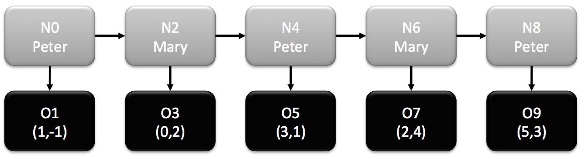
Figure 1: The Take-Or-Leave game (n is odd)

This type of game has often been used to describe the Backwards Induction Paradox in literature (see Section 4.1).

2.1.2 Assurance game

The assurance game (see Fig. 2) models a basic, asynchronous, Pareto-improving exchange in economics (payoffs are utilities). The rule is as follows. First, Peter has the choice between deviating (D - both players get $0$) and cooperating (C). If Peter cooperates, then Mary has the choice between cooperating as well (C), in which case both players get $1$, and deviating (D), in which case Mary gets $2$ and Peter gets $-1$.

Figure 2: The assurance game

This can be interpreted as the possibility for Peter to trust Mary or not, and if he does trust her, Mary can choose to cooperate or not.

2.1.3 $\Gamma$-game

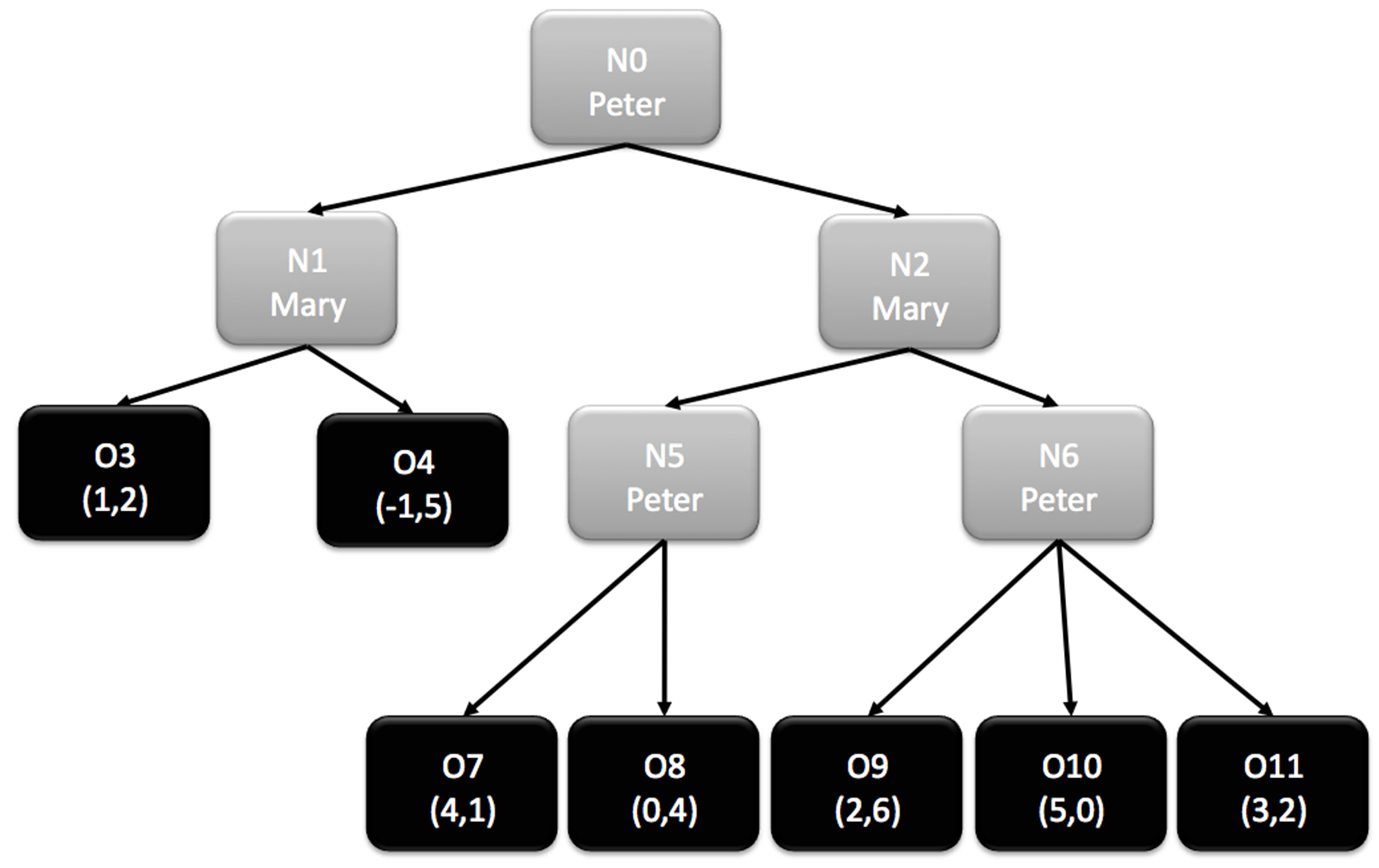
Figure 3: The $\Gamma$-Game

The $\Gamma$-game (see Fig. 3) aims at demonstrating how the PPE is computed on a slightly more complex game. First, Peter has the choice between two nodes. If he chooses $n_{1}$, then Mary chooses between two outcomes; if he chooses $n_{2}$, Mary chooses between two nodes and it is Peter’s turn again. This game does not have a particular interpretation - it was simply designed for the reasoning to be interesting and to help the reader understand how the Perfect Prediction Equilibrium works on general trees.

2.2 Newcomb’s Problem

Newcomb’s problem (Gardner, 1973) is an illustration of how the concepts of prediction and decision interact, and a good starting point to introduce Perfect Prediction. In particular, it is a very good test for distinguishing between agents with two kinds of rationalities that differ by the correlation, or absence thereof, between prediction and decision. Historically, Newcomb’s problem, through the research and literature around it, is actually at the origin of the discovery of these two kinds of rationalities, which is why, in this paper, we decided to call them one-boxer rationality and two-boxer rationality, the latter being the one commonly accepted as game-theoretical perfect rationality. The use of these names, however, by no means reduces the scope of these rationalities to Newcomb’s problem and alternate names are suggested in footnote 2.

Imagine two boxes. One, B, is transparent and contains a thousand dollars; the other, A, is opaque and contains either a million dollars or nothing at all. The choice of the agent is either C1: to take only what is in the opaque box, or C2: to take what is in both boxes. At the time that the agent is presented with this problem, a Predictor has already placed a million dollars in the opaque box if and only if he foresaw that the agent would choose C1. The agent knows all this, and he has very high confidence in the predictive powers of the Predictor. What should he do?

A first line of reasoning leads to the conclusion that the agent should choose C1. The Predictor will have foreseen it and the agent will have a million dollars. If he chose C2, the opaque box would have been empty and he would only have a thousand. The paradox is that a second line of reasoning (taken by most game theorists as it is consistent with Nash) appears to lead just as surely to the opposite conclusion. When the agent makes his choice, there is or there is not a million dollars in the opaque box: by taking both boxes, he will obviously get a thousand dollars more in either case. This second line of reasoning applies dominance reasoning to the problem, whereas the first line applies to it the principle of maximization of expected utility.

The paradox can be solved as follows (although, to be fair, there is to date no established consensus about it). Two-boxers assume that the choice and the prediction are counterfactually independent of each other. In other words, once the prediction is made, the choice is made independently and the prediction, which lies in the past, is held for fixed. Even if the prediction is correct (the player gets $ 1,000), it could have been made wrong (she would have gotten $ 0). One-boxers assume on the contrary that the prediction and the choice are counterfactually dependent. In other words, the prediction is correct (player gets $ 1,000,000), and if the player had made the other choice, the predictor would have correctly anticipated this other choice as well (she would have gotten $ 1,000).

One-boxers and two-boxers are both rational: they merely make different, not to say opposite, assumptions. This illustrates that there are at least two ways of being rational.

A probabilistic illustration along the same lines as this solution has recently been given by Wolpert and Benford (2013). Technically, counterfactual dependence means statistical dependence if events and decisions are seen as random variables. It is a symmetrical relation and ignores the arrow of time (unlike causal dependence).

The Subgame Perfect Equilibrium makes the (“two-boxer”) assumption that decisions are counterfactually independent of the past. More generally, Nash Equilibria make the (“two-boxer”) assumption that the other players’ strategies are held fixed while a single player optimizes her strategy. Perfect Prediction Equilibria, on the other hand, relies on the “one-boxer” assumption of counterfactual dependency. In both cases, players are rational and maximize their utility to the best of their logical abilities. They are, however, rational in two different ways.

2.3 Transparency and Perfect Prediction

In classical game theory (Nash equilibrium), two-boxer-rational agents know that they are rational, know that they know, etc. This is called common knowledge (CK) of rationality in literature. Common knowledge is a form of transparency. In the case of SPE, the possible futures are each considered by, and are transparent to, the current player, for him to decide on his next move.

However, this transparency does not hold the other way round. The player being simulated or anticipated in a possible future – first and foremost, in a subgame that is not actually on the path to the SPE – cannot be fully aware of the rest of the game (that is, of the overall SPE), as this knowledge would be in conflict with the fact of being playing in the subgame at hand. The past is opaque to her, meaning that she cannot be fully aware of the past thought processes. She simply assumes that the past leading to her subgame is fixed, and the other player knows that she does (CK of two-boxer-rationality). This is one-way transparency. Section 4.1 goes into more details on what is known as the backward induction paradox.

It goes otherwise for one-boxer-rational agents. In a game played by one-boxer-rational agents, there is common knowledge of rationality as well, in that players know (and know that they know, etc) that they both react to their knowledge in their best interest. But there is more importantly CK of one-boxer-rationality, which means that (i) each player considers himself to be transparent to the past, in that they integrate this very CK of one-boxer-rationality in their reasoning and consider themselves to be predictable, and (ii) each player P considers himself to be transparent to the future as well, in that they know that a future player F considers player P’s moves to correlate (counterfactually) with their (F’s) decision, whichever way F decides.

This more stringent form of transparency drastically changes the reasoning: since transparency goes both ways, the entire solution of the game (all thought processes, the equilibrium, etc) is CK. In such a perfectly transparent world, each agent would have the same knowledge of the world as an external omniscient spectator, this fact being CK among the agents . The players (profactually) predict the solution correctly, and would also have (counterfactually) predicted it correctly if it had been different. This is what we call Perfect Prediction. This different relation to time was called Projected Time (and the widespread relation to time Occurring Time) by Dupuy (2000).

Rather than considering all possible futures, the one-boxer-rational agents assume that there is one solution of the game that is CK, and based on this assumption, compute and find that very solution of the game that is CK. The players react to their CK of the outcome of the game, play accordingly and reach an outcome which is indeed the predicted outcome. This is nothing else than a fixpoint problem, which can be solved and which has a unique solution, as demonstrated in this paper.

A side effect of assuming CK of the game solution is that the construction of the equilibrium in this paper is supported by reasoning only on the equilibrium path. There is one timeline, and it is completely transparent to itself, by its definition as a fixpoint.

2.4 Two principles behind the computation of the Perfect Prediction Equilibrium

A Perfect Prediction Equilibrium is a path on the tree which can be reached under the assumption of total transparency, or, in other words, by one-boxer rational players that genuinely believe that there is total transparency.

The computation of PPEs by the players or an external game theorist, which is the same, is done by eliminating outcomes of the game which lead to a contradiction (Grandfather Paradox), i.e., which cannot possibly be commonly known as the equilibrium.

At each step of the reasoning, there is CK of the outcomes which are logically impossible (this is part of the thought process). Using this knowledge, it is possible to discard additional outcomes which cannot be commonly known as the equilibrium reached by the game, thanks to the two principles.

2.4.1 First principle

The CK of the outcomes which have been proven logically impossible as well as the assumed CK of the outcome $o$ reached by the game give the players a power of preemption; a player will deviate from the path connecting the root to $o$ (we call this path causal bridge) if the deviation guarantees to him a better payoff than $o$ (whatever the continuation of the game after the deviation can be, and taking into account that some outcomes have been proven logically impossible).

If such is the case, then $o$, which is not a fixpoint, cannot be commonly known as the solution and is logically impossible; it is said to be preempted . We call preemption this process of breaking the causal bridge in reaction to the anticipation of an outcome (see Fig. 4).

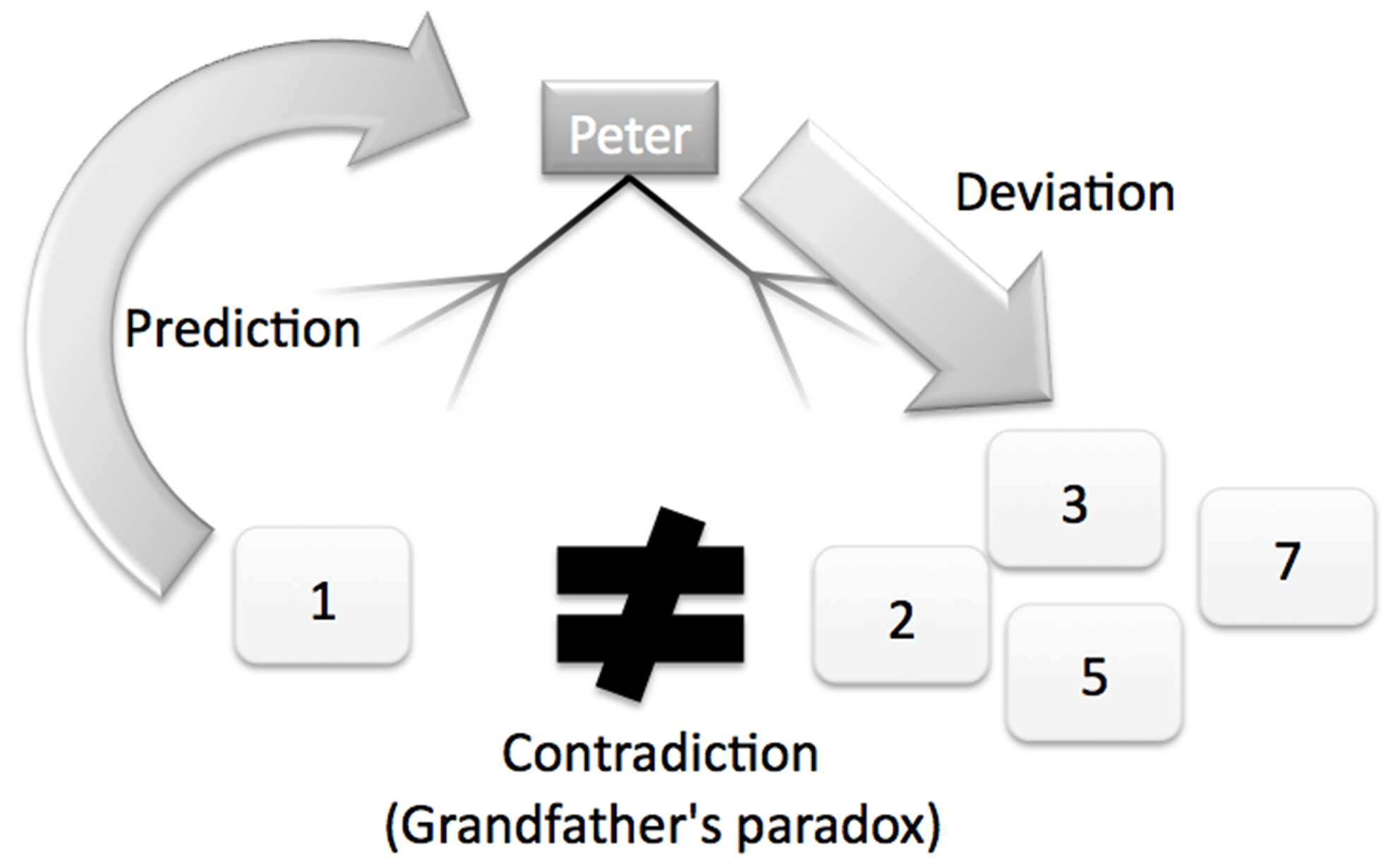
Figure 4: Illustration of the First Principle

Example 1

Let us take $o_{3}$ in the assurance game (Fig. 2). There are no outcomes proven impossible yet. We assume that $o_{3}$ is the outcome eventually reached by the game, which is known to the players. For Peter playing at the root, a deviation from $n_{2}$ (which is on the path leading to $o_{3}$) to $o_{1}$ guarantees him a better payoff (0) than what he gets with $o_{3}$ (-1). This means that anticipating $o_{3}$, Peter deviates and breaks the causal bridge leading to $o_{3}$. Hence, $o_{3}$ cannot be the solution: it is not possible for Peter to predict $o_{3}$ and to play towards $o_{3}$. $o_{3}$ is preempted and is logically impossible. It can be ignored from now on.

Example 2

In the $\Gamma$-game example, $o_{4}$ can also be discarded this way: For Peter playing at the root, a deviation from $n_{1}$ (which is on the path leading to $o_{4}$) guarantees him a better payoff (4, 0, 2, 5 or 3) than what he gets with $o_{4}$ (-1). $o_{4}$ is preempted and can also be ignored from now on.

Principle 1

Let $I$ be the set of the outcomes that have not been discarded yet. The discarded outcomes are ignored. Let $n$ be a given node which is reached by the game and where player $p$ is playing. Let $o\in I$ be an outcome among the descendants of $n$. $o$ is said to be preempted if all outcomes in one of the non-empty subtrees at $n$, give to $p$ a greater payoff than $o$. A preempted outcome is logically impossible, is hence discarded and must be ignored in the remainder of the reasoning.

2.4.2 Second principle

In the assurance game (Fig. 2), given the knowledge that $o_{3}$ is logically impossible, Peter is faced with the choice between $o_{1}$, which gives him 0, and $n_{2}$, which gives him eventually for sure 1 since $o_{3}$ cannot be chosen. Because he is rational, he chooses $n_{2}$. This is the second principle (see Fig. 5).

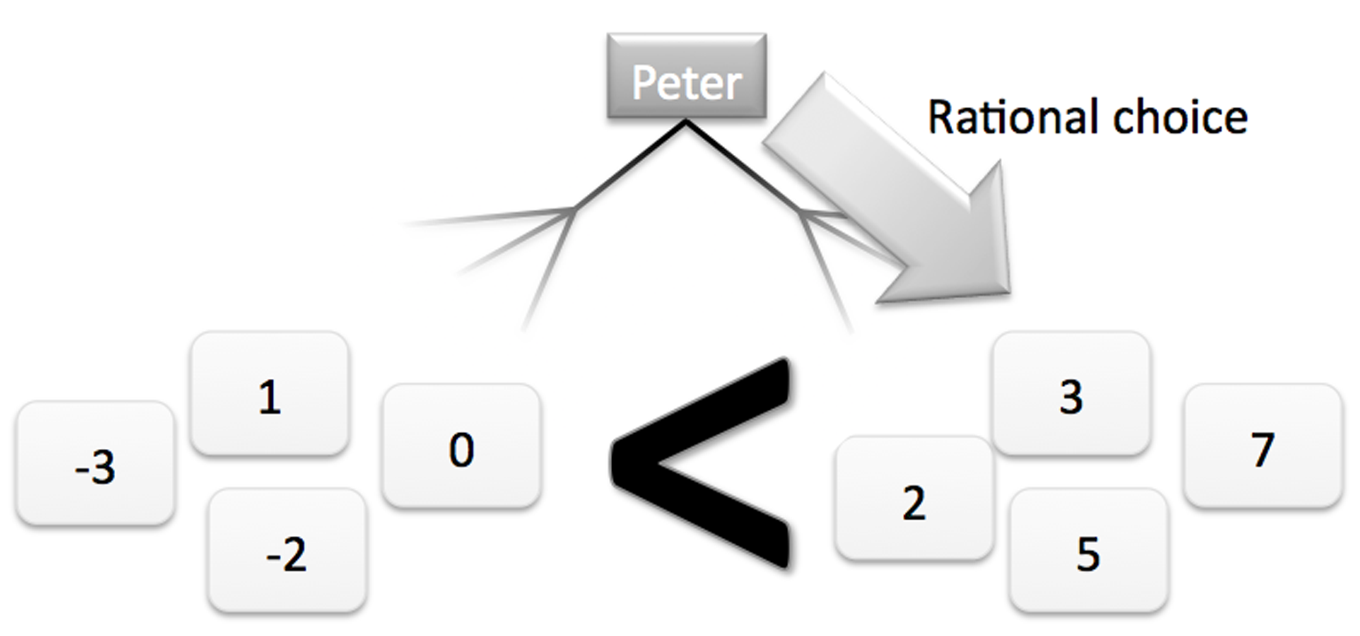
Figure 5: Illustration of the Second Principle

Principle 2

Let $I$ be the set of the outcomes that have not been discarded yet. The discarded outcomes are ignored. Let $n$ be a given node which is reached by the game and where player $p$ is playing. If all outcomes in one of the non-empty subtrees at $n$, of root $r$, are better than any other outcome in the other subtrees, then $p$ chooses $r$. As a consequence, $r$ is also reached by the game, and all remaining outcomes in other subtrees than the one at $r$ are discarded.

The second principle is only applicable if all outcomes on the one side are better than all outcomes on the other side. If the payoffs are “interlaced”, it does not apply - but in this case, the first principle can be used instead.

Also, the second principle applies in the degenerate case where there is only one unique non-empty subtree. Then the player chooses this subtree.

2.4.3 The reasoning to the equilibrium

Based on the two principles, it is possible to build a system of first-order-logic equations for each game, as described in the annex (Section 10.5). By definition, a PPE is a solution to this system. The equations are divided into three groups:

1. Application of the First Principle

2. Application of the Second Principle

3. Causal bridge enforcement (i.e. an equilibrium must be a consistent path starting from the root)

This system can be solved with a technique which turns out to be a forward induction: one starts at the root, discards all outcomes preempted at this step with the first principle, then moves on to the next node - there is always exactly one - with the second principle (this node is now known to be reached by the game), discards all outcomes preempted at this step with the first principle, moves on to the next node with the second principle, etc., until an outcome is reached.

In the reasoning, the list of logically impossible outcomes is initially empty and grows until no more outcomes can be discarded. In fact, as will be proven in Section 3, under the assumption of strict preferences, exactly one outcome remains. The one-boxer rational players have no interest in deviating from the path leading to it and will play towards it: it is the Perfect Prediction Equilibrium, which always exists and is unique.

This system of equations can be described formally, however for pedagogical reasons, from now on, we will reason directly by performing outcome eliminations.

The reasoning is totally transparent and can be performed, ahead of the game or without even playing, by a game theorist or any player, always leading to the same result. Actually, as the structure of the reasoning is a forward induction, it would even be possible to perform the reasoning as you go during the game.

2.5 Computation of the Perfect Prediction Equilibrium for the three examples

We now show how the forward induction reasoning described above can be applied to the examples.

2.5.1 Assurance game (Fig. 2)

We begin at the root.

Being Perfect Predictors, the players at the root cannot predict $o_{3}$ as the final outcome because of the first principle: the prediction of $o_{3}$ would lead Peter to deviate at the root towards $o_{1}$, which invalidates this very prediction. We say that outcome $o_{3}$ has been preempted by the $o_{1}$ move. Therefore, outcome $o_{3}$ has been identified as not being part of the solution: it cannot be commonly known as the outcome reached by the equilibrium and is ignored from now on.

This can also be formulated as a reasoning in Mary’s mind. She is one-boxer rational. Mary includes Peter’s past move as a reaction function to her choice between $o_{3}$ and $o_{4}$. Were she to pick $o_{3}$, Peter would have anticipated it as the rational thing for her to do – and he would have picked $o_{1}$. But this would be inconsistent with her playing at $n_{2}$. Since picking $o_{3}$ is correlated with a past reaction (to the anticipation of $o_{3}$) that is incompatible with $o_{3}$ (Grandfather’s Paradox), she cannot (one-boxer)-rationally pick $o_{3}$.

Now that $o_{3}$ is (identified as being) impossible, we are left with $o_{1}$ and $o_{4}$, and we can apply the second principle: Peter knows that Mary is one-boxer rational and will not pick $o_{3}$. He can either move to $o_{1}$ and win 0, or move to $n_{2}$ and win 1. He chooses the latter and $n_{2}$ is known to be reached by the game.

At $n_{2}$, Mary, according to a trivial application of the second principle (she can only choose $o_{4}$), moves to $o_{4}$, which is known to be reached by the game: it is the only remaining outcome. If there is an equilibrium, it is $o_{4}$.

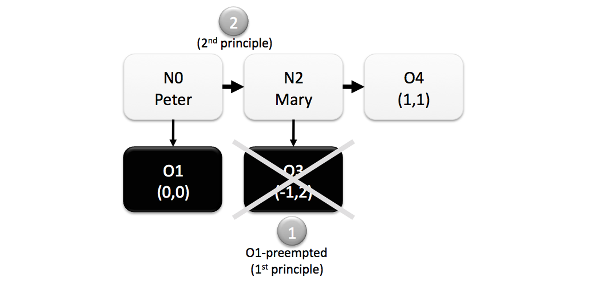
Figure 6: The Perfect Prediction Equilibrium in the Assurance Game

Conversely, it is possible to check that this outcome corresponds to an equilibrium. Predicting $o_{4}$, Peter will not deviate: according to the second principle, he moves to $n_{2}$, i.e., towards $o_{4}$. Mary will not deviate either, since she cannot choose $o_{3}$, which is preempted. More precisely, she forbids to herself to pick $o_{3}$ because her reasoning as a one-boxer rational player stamped it as an illogical move. Like a self-fulfilling prophecy, $o_{4}$ is reached by the game: it is the equilibrium (Fig. 6).

2.5.2 Take-Or-Leave game (Fig. 1)

The previous reasoning can easily be generalized to the Take-Or-Leave-game (Fig. 1).

One begins at the root. The application of the first principle here leads to the preemption of $o_{3}$ because it would be in the interest of Peter to deviate at node $n_{0}$ towards $o_{1}$.

Then, knowing this, according to the second principle, Peter chooses $n_{2}$, since all remaining outcomes in this subtree are better (3, 2, 5) than $o_{1}$ (1), which is discarded.

At $n_{2}$, Mary has to take $n_{4}$ since $o_{3}$ was proven logically impossible (again, her line of reasoning as a one-boxer rational player tells her that it would not be a rational choice).

Then the application of the first principle here leads to the preemption of $o_{7}$ because it would be in the interest of Peter to deviate at node $n_{4}$ towards $o_{5}$.

Then, knowing this, according to the second principle, Peter chooses $n_{6}$, since all remaining outcomes in this subtree are better (5) than $o_{5}$ (3), which is discarded.

At $n_{6}$, Mary has to take $n_{8}$ since $o_{7}$ was proven logically impossible.

At $n_{8}$, Peter chooses the remaining outcome $o_{9}$, which is the Perfect Prediction Equilibrium (Fig. 7).

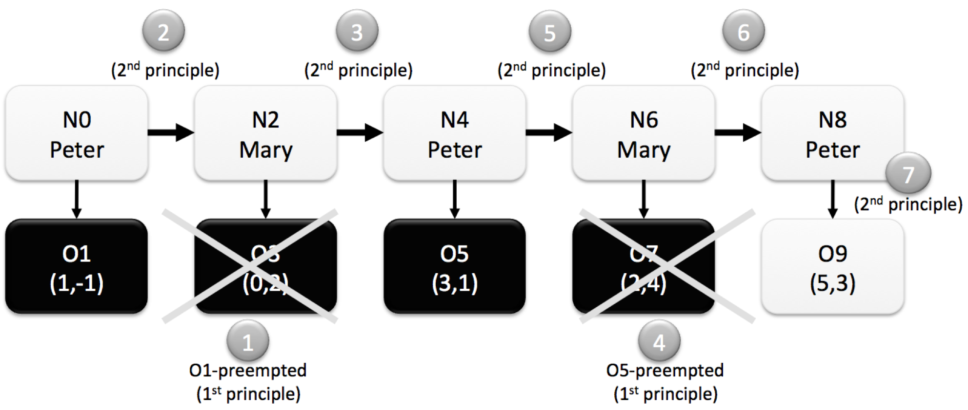
Figure 7: The Perfect Prediction Equilibrium in the Take-Or-Leave game (n is odd)

2.5.3 $\Gamma$-game (Fig. 3)

In this game, the general technique for computing the Perfect Prediction Equilibrium becomes visible.

We start at the root, where the first principle leads to the preemption of $o_{4}$ (Peter would deviate to $n_{2}$ where all payoffs are higher than -1) and then to the preemption of $o_{8}$ (Peter would deviate to $n_{1}$ where all remaining payoffs are now higher than 0).

Since the payoffs are no longer interlaced, we can now apply the second principle. Peter chooses $n_{2}$ (remaining payoffs: 2, 3, 4, 5) over $n_{1}$ (1): $n_{2}$ is now known to be reached by the game, $o_{3}$ is discarded (see Fig. 8).

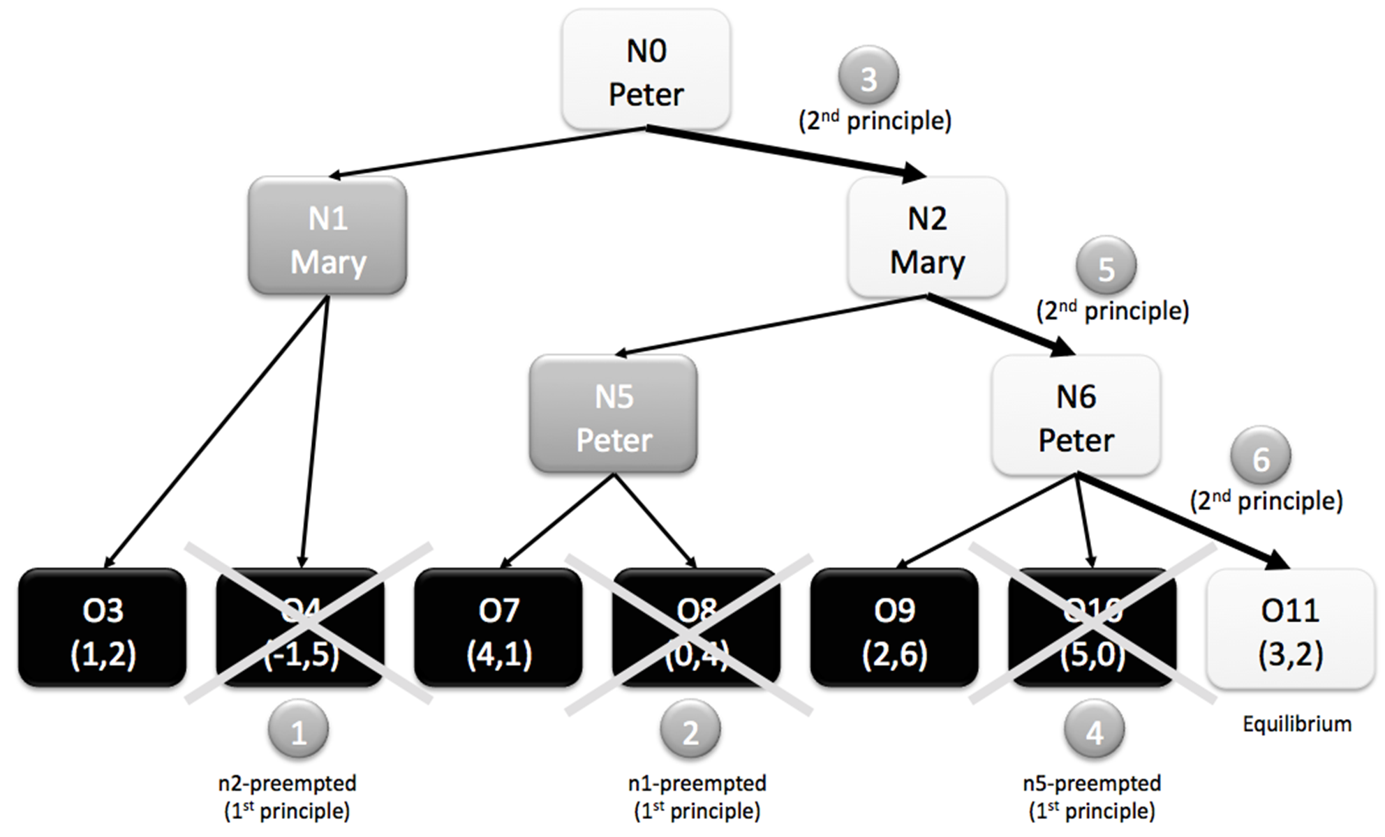
Figure 8: The Perfect Prediction Equilibrium in the $\Gamma$-game

At $n_{2}$ (where the only remaining outcomes are $o_{7}$, $o_{9}$, $o_{10}$ and $o_{11}$), we apply the first principle with Mary: $o_{10}$ is preempted (Mary would deviate to $n_{5}$). Then the second principle applies: Mary chooses $n_{6}$ (2, 3) over $n_{5}$ (1). $n_{6}$ is known to be reached by the game, $o_{7}$ is discarded.

At $n_{6}$ (where the only remaining outcomes are $o_{9}$ and $o_{11}$), we apply directly the second principle: Peter chooses $o_{11}$ (3) over $o_{9}$ (2).

The game reaches $o_{11}$. Conversely, the players, anticipating this outcome, will play towards it: it is the equilibrium.

In fact, the algorithmic procedure will always be the same: identify the subgame with the worst payoff and preempt its worst outcomes by making use of other subgames as potential deviations.

3 Construction of the Perfect Prediction Equilibrium

3.1 A general definition

In the former section, we introduced Perfect Prediction, the idea of preemption and two principles, and constructed the PPE for some examples. We now define the Perfect Prediction Equilibrium for all games in extensive form, without chance moves and strict preferences.

We assume that both players are one-boxer rational. They consider that the solution to the game is CK.

The application of the two principles detailed in Section 2 allows the elimination of all outcomes but one. The remaining, non-discarded outcome is the Perfect Prediction Equilibrium. It is immune against the CK that the players have of it. The two players, having anticipated it, have no interest in modifying their choices and will play towards this outcome: it is a fixpoint.

Note that the definition of the Subgame Perfect Equilibrium in terms of stability is very similar: it is an equilibrium which is reached when both players have no interest in modifying their strategy, knowing the other player’s strategy, including what he would do at unreached nodes. In our definition however, we never consider unreached nodes: the Perfect Prediction Equilibrium is stable with respect to the knowledge of itself as a path, and only of itself. This implies that, as opposed to the Nash Equilibrium, there is no sense in talking of “equilibria in each subgame”. Actually the different subgames of the tree disappear along the construction of the equilibrium: they are just used as temporary possible deviations.

We believe that the Perfect Prediction Equilibrium fulfills a stability condition which is simpler, more natural and more compact (self-contained) than the Subgame Perfect Equilibrium. It may be regarded as both normative (because the Pareto optimality is an incentive to adopt it in the sense that it never reaches sub-optimal outcomes) and positive (it describes game outcomes encountered in real life, like the assurance game).

3.2 The construction of the Perfect Prediction Equilibrium

We consider two-player finite games with perfect information, without chance moves and with strict preferences.

Definition 1

(Labeled tree) A labeled tree is a tree whose root is $n_{0}$, and such that:

- each node $n$, labeled by a player $p_{n}$, has a set $F(n)$ of offsprings (nodes or outcomes).

- each leaf is an outcome $o$ labeled by a couple of integers ($a^{Peter}_{o},a^{Mary}_{o}$).

- all $(a^{Peter}_{o})_{o}$ are distinct and all $(a^{Mary}_{o})_{o}$ are distinct

The label $p_{n}$ at node $n$ indicates whose turn it is to play. The offsprings $F(n)$ of node $n$ are player $p_{n}$’s possible choices.

The label $(a^{Peter}_{o},a^{Mary}_{o})$ at outcome $o$ indicates how much Peter and Mary get.

For convenience, nodes and outcomes are numbered ($n_{0}$, $n_{1}$ or $o_{1}$, $n_{2}$ or $o_{2}$, …) so that it is possible to easily refer to them in the examples.

The last part of the definition corresponds to the assumption that each player has a strict preference between any two outcomes.

We define $D(n)$ as the set of all descendants (nodes and outcomes) of node $n$; it is the transitive and reflexive closure of the offspring-relation.

To compare outcomes, we write that $o_{1}<_{p}o_{2}$ whenever $a^{p}_{o_{1}}<a^{p}_{o_{2}}$. When the player is clear from the context, we will also say that an outcome is better or worse than another one (meaning for the current player).

Example 3

In the Assurance game, we have two nodes, $n_{0}$ (the root) and $n_{2}$, and three outcomes $o_{1}$, $o_{3}$ and $o_{4}$. The players are $p_{n_{0}}=$Peter and $p_{n_{2}}$=Mary. F is defined as $F(n_{0})=\{o_{1},n_{2}\}$ and $F(n_{2})=\{o_{3},o_{4}\}$. The payoffs are $(a^{Peter}_{o_{1}},a^{Mary}_{o_{1}})=(0,0)$, $(a^{Peter}_{o_{3}},a^{Mary}_{o_{3}})=(-1,2)$ and $(a^{Peter}_{o_{4}},a^{Mary}_{o_{4}})=(1,1)$. Peter’s payoffs are all distinct, as well as Mary’s payoffs. D is defined as $D(n_{0})=\{o_{1},n_{2},o_{3},o_{4}\}$ and $D(n_{2})=\{o_{3},o_{4}\}$.

A very short summary of the construction of the Perfect Prediction Equilibrium is the following: the reasoning is done by discarding all outcomes which cannot be CK. We start at the root. The outcomes in all direct subtrees but one are discarded, as well as some outcomes in the remaining subtree. The next move has to be the root of the only subtree where at least one outcome remains. Hence, the next move exists and is unique (Lemma 1). We continue with the next move and so on, until an outcome is reached, which is the outcome of the Perfect Prediction Equilibrium.

3.2.1 Initialization, notations: $c_{i}$ and $I_{i}$

An equilibrium is a path $(c_{i})_{i=1..d}$ such that the first player starts at $c_{1}=n_{0}$, and at each step $i$, given $c_{i-1}$, the next move is $c_{i}\in F({c_{i-1}})$.

Formally :

• $c_{1}=n_{0}$ (the root)

• $\forall i=1..d-1,c_{i}$ is a node

• $\forall i=2..d,c_{i}\in F(c_{i-1})$

• $c_{d}$ is an outcome

Example 4

In the $\Gamma$-game, the equilibrium is $(c_{1},c_{2},c_{3},c_{4})$ where $c_{1}=n_{0},c_{2}=n_{2},c_{3}=n_{6},c_{4}=o_{11}$.

At each step $i$ we are also given $I_{i-1}$, a subset of the set $D(c_{i-1})$ of the outcomes descending from the previous move $c_{i-1}$. This set $I_{i-1}$ is the set of all outcomes that are immune against their knowledge up to $c_{i-1}$ (technically speaking, they have not been discarded yet: the second principle has only been applied up to $c_{i-1}$, their common ancestor, and they could not be preempted with the first principle at any node earlier on the path).

Example 5

In the $\Gamma$-game, the sequence would be $I_{1}=\{\textbf{all outcomes}\}$, $I_{2}=\{o_{7},o_{9},o_{10},o_{11}\}$, $I_{3}=\{o_{9},o_{11}\},I_{4}=\{o_{11}\}$. $o_{7}$ is in $I_{2}$ because it is not discarded, meaning that if Peter at $c_{1}=n_{0}$ anticipates $o_{7}$, he will not deviate. $o_{8}$ does not make it in $I_{2}$ because it is preempted by Peter at $n_{0}$ according to the first principle. $o_{3}$ is not in $I_{2}$ either since it is discarded by the second principle, as well as all outcomes not in the $n_{2}$ subtree.

A node that is not in $I_{i-1}$ cannot be commonly known to be reached by the game, either because it was discarded by the second principle, or because it would bring about a deviation in the past according to the first principle. Note that sometimes, when the outcomes in two subtrees are not interlaced, it can be ambiguous which principle to apply to discard some outcomes: when the second principle potentially selects a subtree and discards the other outcomes, then the first principle could also be used instead to preempt the very same outcomes with this subtree. This leaves room for a philosophical interpretation (preemption or rational choice), but does not change what outcomes are discarded. This is why, in this section, we will apply the first principle whenever it applies, and then the second principle, but we will push forward the word “discard” instead of “preempt” to leave open which principle is used in the interpretation.

Example 6

In the $\Gamma$-game, one could also argue that $o_{3}$ is not in $I_{2}$ by invoking the first principle: $o_{3}$ is preempted by the $n_{2}$ move. Even with this interpretation, it changes nothing to the fact that all outcomes not in the $n_{2}$ subtree are discarded.

In other words, the outcomes that are not in the set $I_{i-1}$ are not to be taken into account anymore: they have been proven not to fit the definition of the equilibrium. The other partially fit the definition: they are immune against their knowledge at least up to $c_{i-1}$, which means that players will play towards this outcome at least until $c_{i-1}$ is reached, but could still deviate later.

At the beginning $I_{1}=\{$all outcomes$\}$, which means that no outcome has been discarded yet: $c_{1}$ is the root and is always reached because the game starts here (the causal bridge is secured).

At each step, we discard outcomes (with the first principle, or possibly the second principle for the very last discarding, which is technically equivalent) until all subtrees but one are completely discarded, and finish with the second principle which allows us to move on to the next node and the next step.

3.2.2 Newcombian States

At step $i$, the last move $c_{i-1}$ and the remaining outcomes $I_{i-1}$ are given. For example at step $2$, the last move is the root ($c_{1}=n_{0}$) and the remaining outcomes are all the outcomes ($I_{1}=\{$all outcomes$\}$), and we are looking for $c_{2}$ and $I_{2}$.

We will now define Newcombian States for the player $p_{c_{i-1}}$ (the current player) so as to recursively determine the outcomes that are not immune against their common knowledge because of a deviation at the node $c_{i-1}$. These outcomes are discarded at this step.

A Newcombian State has a pure part (corresponding to a possible move) and a discarding part (a Newcombian State which invalidates some outcomes as equilibrium candidates, with one of the two principles). It can be thought of as a bundle containing a move (its “pure part”) together with the knowledge and the proof (its “discarding part”) that some of its descendant outcomes are impossible. The proof that such an outcome is impossible consists of a witness: the move in the discarding part

• to which the player $p_{i-1}$ would deviate according to the first principle if the outcome were predicted.

• or to which the player $p_{i-1}$ actually goes according to the second principle.

Definition 2

(Newcombian State, pure part, discarding part) At step $i$, a Newcombian State of order $k$, with $k\geq 1$, is an element $\eta=(\eta_{1},..,\eta_{k})\in{(F(c_{i-1}))}^{k}$, constituted by offsprings of the last move, such that any two consecutive elements are different:

$$\eta=(\eta_{1},..,\eta_{k})\in{(F(c_{i-1}))}^{k}:\eta_{j}\neq\eta_{j+1},\quad j=1..k-1$$ (1)

The pure part of a Newcombian State is its first element: $\mathbf{pure}(\eta)=\eta_{1}\in F(c_{i-1})$.

The discarding part of a Newcombian State of order $k>1$ is the element of $({F(c_{i-1})})^{k-1}$ composed by the $k-1$ last elements of $\eta$:

$$\mathbf{discard}(\eta)=(\eta_{2},..,\eta_{k})\in{(F(c_{i-1}))}^{k-1}$$

.

Example 7

In the $\Gamma$-game, $(n_{1},n_{2})$ is a Newcombian state of order 2. Its pure part is $n_{1}$ and its discarding part is $n_{2}$. $n_{2}$ is a witness that a descendant ($o_{4}$) of $n_{1}$ is impossible, because it is discarded by the first principle ($o_{4}$ is preempted by $n_{2}$).

Likewise, $(n_{2},n_{1},n_{2})$ is a Newcombian state of order 3. Its pure part is $n_{2}$ and its discarding part is $(n_{1},n_{2})$. The latter is a witness that a descendant ($o_{8}$) of $n_{2}$ is discarded by the first principle (it is preempted by $n_{1}$ knowing that $o_{4}$ is impossible).

Finally, $(n_{1},n_{2},n_{1},n_{2})$ is a Newcombian state of order 4. Its pure part is $n_{1}$ and its discarding part is $(n_{2},n_{1},n_{2})$. The latter is a witness that a descendant of $n_{1}$ ($o_{3}$) is impossible. In this case, it is open whether the second principle (Peter chooses $n_{2}$, knowing that $o_{8}$ and $o_{4}$ are impossible, which discards all outcomes in other subtrees) or the first principle ($o_{3}$ is preempted by $n_{2}$ knowing that $o_{8}$ and $o_{4}$ are impossible) is applied, liked we mentioned above. Whichever principle is used, $o_{3}$ is discarded.

A Newcombian State of order 1 is a pure Newcombian State: no outcome has been discarded yet (unless it was at a former step, but we said that outcomes invalidated at a former step are out of the race anyway).

Example 8

$(n_{2})$ is a pure Newcombian state, i.e., in which no outcomes have been discarded yet.

3.2.3 Target function and discarding

Each Newcombian State is associated with the subset of the descendants of its pure part that are not discarded by its discarding part. This is defined recursively by making appeal to the target function $T_{i}$ in the following way:

Definition 3

(Target function and Discarding) At step $i$,

- if $\eta$ is a first-order Newcombian State, i.e. $\eta=(\eta_{1})$, then $T_{i}(\eta)$ is the set of outcomes that are among the descendants of $\eta_{1}$ and that were not discarded before step $i$:

$$T_{i}(\eta)=I_{i-1}\cap D(\eta_{1})$$

- if $\eta$ is a Newcombian State of order $k>1$, i.e. $\eta=(\eta_{1},p)$, then $T_{i}(\eta)$ is the set of outcomes that are among the descendants of $\eta_{1}$ and that were not discarded before step $i$, excluding outcomes worse than the worst outcome in $T_{i}(p)$ if $T_{i}(p)$ is not empty.

Every outcome that is excluded that way is called $p$-discarded. Any outcome in $T_{i}(\eta)$ is said $\mathbf{\eta}$-targeted. If we denote the set of the $p$-discarded outcomes with

$$P_{i}(p)=\{o\in I_{i-1}\setminus D(\textbf{pure}(p))|T_{i}(p)\neq\emptyset\wedge\forall o^{\prime}\in T_{i}(p),o<_{p_{c_{i-1}}}o^{\prime}\}$$

then

$$T_{i}(\eta)=(I_{i-1}\cap D(\eta_{1}))\setminus P_{i}(p)$$

which defines a recursion on $k$.

Note the terminology: an outcome is discarded by a Newcombian State.

The operation of discarding corresponds to the player’s behavior described in the principles:

• With the first principle, if, predicting outcome $o$ will happen, she moves to a subtree with outcomes that are all better than $o$, then $o$ is discarded and is no longer an equilibrium candidate.

• With the second principle, the player selects a move, which discards any outcome in the other subtrees.

Example 9

For example in the $\Gamma$-game, at the root, i.e. step 2, the target functions for the pure Newcombian states are $T_{2}(n_{1})=\{o_{3},o_{4}\}$ and $T_{2}(n_{2})=\{o_{7},o_{8},o_{9},o_{10},o_{11}\}$ (they contain all descendants). The corresponding discarding functions are $P_{2}(n_{1})=\emptyset$ and $P_{2}(n_{2})=\{o_{4}\}$. Knowing this, it is possible to compute the target functions of the Newcombian states of order 1: $T_{2}(n_{2},n_{1})=T_{2}(n_{2})\setminus P_{2}(n_{1})=T_{2}(n_{2})$ and $T_{2}(n_{1},n_{2})=T_{2}(n_{1})\setminus P_{2}(n_{2})=\{o_{3},o_{4}\}\setminus\{o_{4}\}=\{o_{3}\}$.

There are two extreme cases for discarding:

• If $T_{i}(p)=\emptyset$, or if there is no $\eta_{1}$-targeted outcome worse than the worst $p$-targeted outcome, then $T_{i}(\eta)=T_{i}(\eta_{1})$. Discarding $\eta_{1}$-targeted outcomes by $p$ is ineffective.

• If all $\eta$-targeted outcomes are worse than the worst $p$-targeted outcome, then $T_{i}(\eta)=\emptyset$. This time, discarding the descendance of $\eta_{1}$ by $p$ is at its highest efficiency, since $p$ discards every $\eta_{1}$-targeted outcome. $\eta$ is called a degenerate state. A degenerate state cannot discard any outcome.

  It is only for a degenerate state $\eta$ that it is ambiguous which principle is being applied: the first one (the outcomes in $P_{i}(p)$ are preempted) or the second one (the player moves rationally to the pure part of $\eta$). For non-degenerate states, only the first principle makes sense.

3.2.4 Example

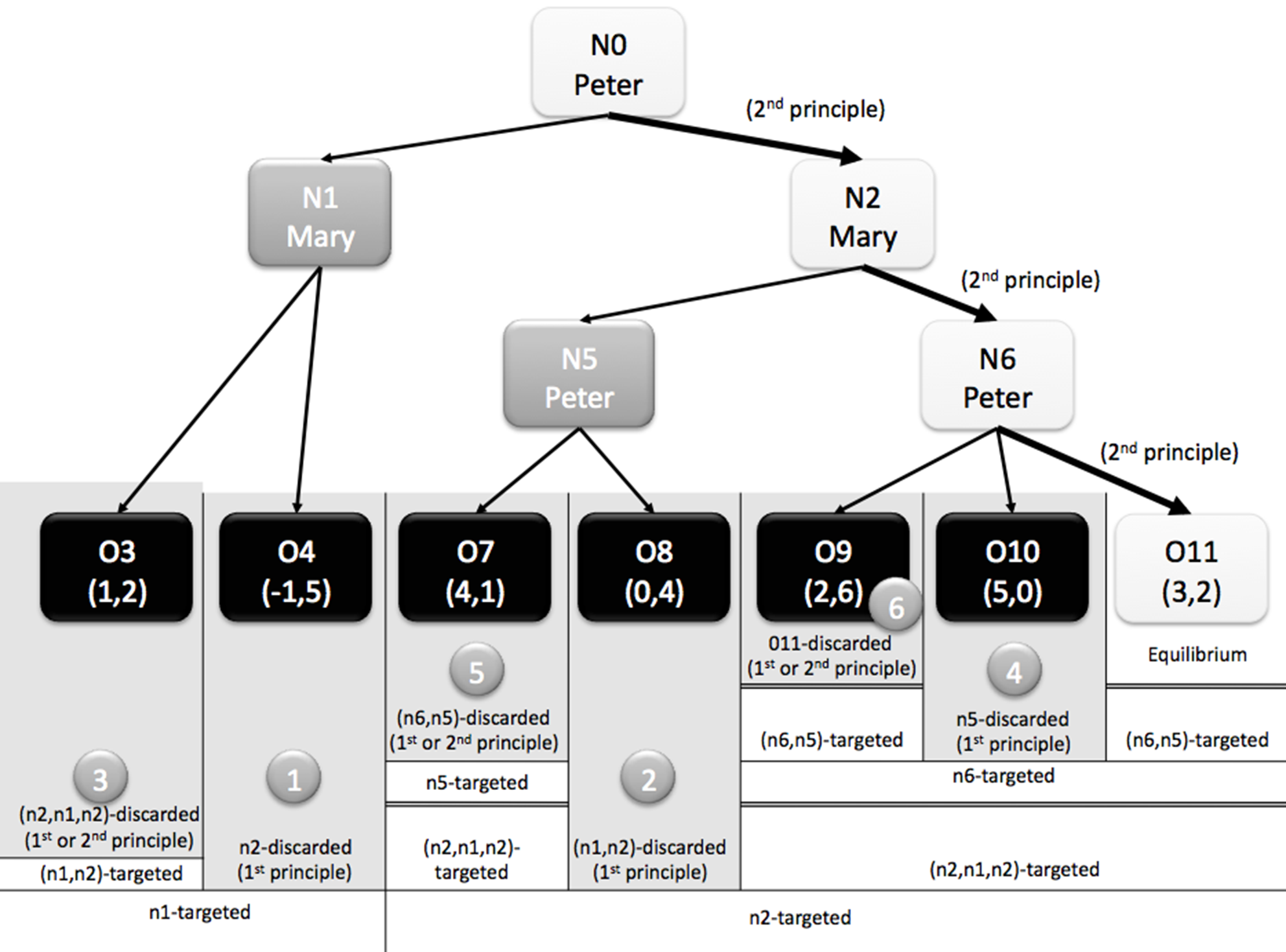
Figure 9: The $\Gamma$-game with Newcombian states and their targeted/discarded outcomes at the root.

At step $1$ of game $\Gamma$, we have $c_{1}=n_{0}$ and $I_{1}=\{$all outcomes$\}$ (initial values).

At step $2$, we compute the target functions of the Newcombian States:

$$T_{2}(n_{1}) = \{o_{3},o_{4}\}$$

$$T_{2}(n_{2}) = \{o_{7},o_{8},o_{9},o_{10},o_{11}\}$$

$$P_{2}(n_{1}) = \emptyset$$

$$T_{2}(n_{2},n_{1}) = T_{2}(n_{2})$$

$$P_{2}(n_{2}) = \{o_{4}\}$$

$$T_{2}(n_{1},n_{2}) = T_{2}(n_{1})\setminus P_{2}(n_{2})=\{o_{3},o_{4}\}\setminus\{o_{4}\}=\{o_{3}\}$$

$$P_{2}(n_{1},n_{2}) = \{o_{8}\}$$

$$T_{2}(n_{2},n_{1},n_{2}) = T_{2}(n_{2})\setminus P_{2}(n_{2})$$

$$= \{o_{7},o_{8},o_{9},o_{10},o_{11}\}\setminus\{o_{8}\}=\{o_{7},o_{9},o_{10},o_{11}\}$$

$$P_{2}(n_{2},n_{1},n_{2}) = \{o_{3},o_{4}\}$$

$$T_{2}(n_{1},n_{2},n_{1},n_{2}) = T_{2}(n_{1})\setminus P_{2}(n_{2},n_{1},n_{2})=\{o_{3},o_{4}\}\setminus\{o_{3},o_{4}\}=\emptyset.$$

The entire reasoning (also at $n_{2}$ and $n_{6}$) is indicated on Fig. 9, where the order of the sub-steps is indicated by the numbers in gray circles. Sub-steps 1, 2 and 3 are performed by Peter at $n_{0}$. One notices that, by discarding all outcomes we can, we are left with outcomes $o_{7}$, $o_{9}$, $o_{10}$ and $o_{11}$, and all of them are descendants of $n_{2}$, which is chosen by Peter ($c_{2}=n_{2}$ and $I_{2}=\{o_{7},o_{9},o_{10},o_{11}\}$). Sub-steps 4 and 5 are then performed by Mary at $n_{2}$ and Sub-step $6$ at $n_{6}$ by Peter. Actually, it always works in the same way, at each step and for any game: we can discard the outcomes of all subtrees but one, as demonstrated in the next part.

3.2.5 The current player’s move

In the example, we saw that after discarding as many outcomes as possible at the root, only outcomes in exactly one subtree remained - this means that this subtree corresponds to the player’s next move. We will now show that at any node reached by the game, the current player’s move exists and is unique.

Having constructed all Newcombian States at step $i$, a certain amount of outcomes, having been discarded, are impossible. We consider all the outcomes that are still available after this: these are the outcomes that are immune against their knowledge up to the current step.

The set $I_{i}\subset I_{i-1}$ of all remaining outcomes is given by:

$$I_{i}=I_{i-1}\setminus(\bigcup_{\eta}P_{i}(\eta))$$

Note that this infinite union is merely a notation, and represents in fact a finite union, since all the $P_{i}(\eta)$ are subsets of $I_{i-1}$ (and the set of subsets of a finite set is finite). Nevertheless, despite being practical, this notation does not allow to create any algorithm for computing the equilibrium. We will present another characterization of the current player’s move which permits this in Section 7.1.2.

Example 10

In the $\Gamma$-game, after reasoning at the root, the set of remaining outcomes is $I_{2}=I_{1}\setminus(P_{2}(n_{1})\cup P_{2}(n_{2})\cup P_{2}(n_{1},n_{2})\cup P_{2}(n_{2},n_{1})\cup...)=\{o_{7},o_{9},o_{10},o_{11}\}$. Note that it is impossible to algorithmically compute the infinite union with this formula, but the result is obtained by noticing that all other outcomes have been discarded, and these four remaining outcomes cannot be discarded by any of the two principles: they are all better for Peter than any outcome in any other subtree.

Lemma 1

Existence and uniqueness of current player’s move

1. (Existence of the current player’s move) There is at least one outcome which has not been discarded during the process:

$$I_{i}=I_{i-1}\setminus(\bigcup_{\eta}P_{i}(\eta))\neq\emptyset$$

2. (Uniqueness of the current player’s move) All remaining outcomes are the descendants of one unique offspring of the last player’s move $c_{i-1}$:

$$\exists!f\in F(c_{i-1}),I_{i}\cap D(f)\neq\emptyset$$

and this very offspring is the current player’s move $c_{i}$:

$$\{c_{i}\}\equiv\{f\in F(c_{i-1}),I_{i}\cap D(f)\neq\emptyset\}$$

Example 11

If we continue with the example above, we see that all remaining outcomes ($o_{7}$, $o_{9}$, $o_{10}$, $o_{11}$) are descendants of $n_{2}$. This implies that $c_{2}=n_{2}$.

Now that all outcomes in all subtrees but one have been discarded, the game reaches $c_{i}$: whatever outcome in $I_{i}$ is anticipated, the players play towards $c_{i}$. Hence, the reasoning can continue at this node, at which further outcomes can be discarded.

3.2.6 End of recursion - Definition and Theorem

When the path reaches an outcome $c_{d}$ ($I_{d}=\{c_{d}\}$), the induction stops, leaving one non-discarded outcome.

Example 12

In the $\Gamma$-game, at step 3, the game reaches $c_{3}=n_{6}$ with the remaining outcomes $I_{3}=\{o_{9},o_{11}\}$. At step 4, it reaches $c_{4}=o_{11}$ with $I_{4}=\{o_{11}\}$. The induction stops here: $o_{11}$ is reached by the game. ($n_{0},n_{2},n_{6},o_{11}$) is the equilibrium: under the assumption of total transparency, the players will reach it; even though they know it in advance, they never deviate. Actually, the fact that they know it in advance causes them to reach it.

Definition 4

(Perfect Prediction Equilibrium) In a game in extensive form represented by a finite tree, with perfect information, without chance moves and with strict preferences between the outcomes, under the assumption of total transparency, a Perfect Prediction Equilibrium is a path leading to a non-discarded outcome, i.e., an outcome which is immune against the CK that the players have of it: the players, anticipating it, have no interest in modifying their choices and do play towards this outcome. It is a fixpoint, in that it follows causally from its prediction.

Theorem 3.1

(Existence and uniqueness of the Perfect Prediction Equilibrium) In a game in extensive form represented by a finite tree, with perfect information, without chance moves and with strict preferences between the outcomes, there is one unique Perfect Prediction Equilibrium.

3.3 Pareto optimality

The Perfect Prediction Equilibrium has the additional property of always being Pareto-optimal. This concept is of crucial importance in economics. In our case, it means that when the PPE is reached, the payoffs are distributed so that no other equilibrium can make a player better off without making the other player worse off.

Theorem 3.2

The outcome of the Perfect Prediction Equilibrium is Pareto-optimal among the outcomes of the game.

Note that, although the PPE is always Pareto-optimal, it is not always a Pareto improvement of the SPE (for a counterexample, see the complete analysis of biped games in the Appendix, case “$1\neq$” with $d=1$ and $f=0$).

4 Related Work

4.1 The Backward Induction Paradox

In the last decades, there has been a debate around the so-called Backward Induction Paradox: CK of rationality is also assumed at nodes that are known to be not reached given this very CK of rationality. This points out that in some way, the SPE is not completely transparent to itself: the players do know their respective strategies, and though cannot be fully – that is, at all nodes in the tree – cognizant of the final equilibrium determined by these two strategies.

One of the motivations behind the Perfect Prediction Equilibrium is to avoid the Backward Induction Paradox (BIP). In this section, we show how literature relates the BIP to the assumption of counterfactual independence and hence, why giving up this assumption circumvents the BIP.

Two kinds of BIPs can be found in literature.

Pettit and Sugden (1989) describe an empirical BIP with the example of the prisoner’s dilemma (a game with imperfect information): “There is a well-known argument – the backward induction argument – to the effect that, in such a sequence, agents who are rational and who share the belief that they are rational will defect in every round. This argument holds however large $n$ may be. And yet, if $n$ is a large number, it appears that I might do better to follow a strategy such as tit-for-tat. […] This is the backward induction paradox.”

Baltag et al (2009) describe a more fundamental, logical BIP as follows: “in order even to start the reasoning, a player assumes that (common knowledge of, or some form of common belief in) rationality’ holds at all the last decision nodes (and so the obviously irrational leaves are eliminated); but then, in the next reasoning step (going backward along the tree), some of these (last) decision nodes are eliminated, as being incompatible with (common belief in) rationality!” Reny (1992) showed that in the Take-or-Leave game, CK of rationality is self-contradictory at each node outside of the equilibrium path.

In the last two decades, the Backward Induction Paradox has been the object of an uninterrupted debate. On the one side, Aumann (1995) proved that “common knowledge of rationality (CKR) implies [that players are reasoning by] backward induction.” (although he does not “claim that CKR obtains or should obtain”). On the other side, Stalnaker states that “Common knowledge of substantive rationality does not imply the backwards induction solution” (Halpern, 2001) and argued (Stalnaker, 1998) that Aumann’s argument “conflates epistemic and causal independence, implicitly making a strong epistemic independence assumption which it explicitly rejects.” The opposition to Aumann’s claim was supported by (Binmore, 1996) and (Binmore, 1997).

Halpern (2001) showed that both sides are right, in that “the key difference between Aumann and Stalnaker lies in how they interpret” the counterfactual’ statement “for all vertices $v$, if the player were to reach vertex $v$, then the player would be rational at vertex $v$” (substantive rationality), i.e., whether it is a material or a counterfactual implication.

Baltag et al (2009) go in another direction by allowing players to have“a moment of temporary irrationality.”

We believe that the Backward Induction Paradox is due to the lack of transparency arising from the widespread assumption that present decisions are counterfactually independent of past moves, an assumption also made explicitly by Baltag et al (2009): “players have no non-trivial “hard” information about the outcomes […]: they cannot foretell the future, cannot irrevocably know the players’ freely chosen future moves (though they do irrevocably know the past, and they may irrevocably know the present […])”.

Perfection prediction theory aims at giving an alternate game-theoretical solution concept with the exact opposite assumption: there is CK of the outcome of the game, and the past is counterfactually dependent on this outcome. There is also CK of rationality on the equilibrium path, and no need for it outside of this path (no counterfactuals on (un)reached nodes, no substantive rationality).

This happens to lead to cooperative, Pareto-optimal behavior. Hence, the Backward Induction Paradox, in the two formulations given above, does not manifest itself in the PPE theory.

Supporting the possibility of having an alternate theory of rational choice, Kreps (2009) argues that “when one says “rational choice theory”, it sounds as if only one theory or model of choice could qualify. How could two distinct theories or models both be rational? But people behave in different ways, depending on the specific context and the more general social situation, and I see no reason to privilege one universal model of behavior with the adjective rational. To do so is, if not demonstrably silly, at least demonstrably misleading.”

4.2 Super-Rationality

Hofstadter (1983) introduced the concept of super-rationality like so: ”Super-rational thinkers, by recursive definition, include in their calculations the fact that they are in a group of super-rational thinkers.” Super-rationality is defined for symmetric games. We believe that the one-boxer rationality underlying the PPE is the equivalent of super-rationality for games in extensive form, as it shares the core idea of transcending rationality, in that players include the knowledge thereof in their calculations.

Shiffrin et al (2009) argue that rationality is ”not a normative concept but rather a social consensus of a sufficiently large proportion of humans judged to be sufficiently expert.” They point out that normative game theory reaches non-(Parent)-efficient optima and initiated research to suggest an alternate equilibrium concept that aims at being Pareto-optimal and that differs from the Nash equilibrium. They explicitly point to Hofstadter’s super-rationality as a starting point. Also, they compare their approach to a single player’s playing against himself under the effect of the Midazolam drug, which makes him forget his past decisions while preserving his reasoning abilities. It can be taken from the draft that, unlike the PPE, no preemption structure is considered. Also, they are facing an exponential explosion of the search space for more than 2 players. The PPE scales to any number of players with the same algorithms.

4.3 Forward Induction

The Perfect Prediction Equilibrium is de facto built with a forward induction, since its construction begins at the root and ends at an outcome. Note that, in game theory, the expression “Forward Induction” carries much more meaning than the fact that the reasoning follows a path from the root to an outcome.

Although in the past many Forward Induction Equilibria have been designed, according to Govindan and Wilson (2008), “the literature provides no formal definition of Forward Induction.”

We now compare our equilibrium with others found in literature by first looking at differences and then at similarities.

First of all, we limit ourselves to games with perfect information, meaning that information sets are all singletons, so that beliefs (as they are defined in the Sequential Equilibria of Kreps and Wilson (1982)) are the trivial function 1 on a singleton.

Additionally, Forward Induction is often used with mixed strategies leading to probability distribution over the game outcomes. Usually, Forward Induction seems to select an equilibrium among the Sequential Equilibria as defined by Kreps and Wilson (1982). In our work we only consider pure strategies, with pure game outcomes.

Finally, there is the issue of what happens outside of the path. It has already been addressed, for example in the Weakly Sequential Equilibrium by Kreps and Wilson (1982), where strategies are required to be optimal only on non-excluded information sets (but are defined also on information sets excluded by these very strategies). Cho and Kreps (1987) introduced signaling games, in which they also address this issue: “If one can restrict the out-of-equilibrium beliefs (or hypotheses) of B, one can sometimes eliminate many of the equilibria.” We find the same idea in the work of Banks and Sobel (1987): “This section presents an equilibrium concept that refines the set of sequential equilibria in signaling games by placing restrictions on off-the-equilibrium-path beliefs”. In our case, pure strategies are simply not defined at all outside the equilibrium path. Actually, outside the equilibrium path, it is not even assumed that players are rational.

In spite of these differences (perfect information, pure strategies, no definition outside of the equilibrium path), we can find some interesting similarities with existing Forward Induction Equilibria.

It is commonly assumed that past play was rational, as opposed to backward induction, where future play only is supposed to be rational. See for example Govindan and Wilson (2008): “Kohlberg and Mertens label this result Forward Induction but they and other authors do not define the criterion explicitly. The main idea is the one expressed by Hillas and Kohlberg in their recent survey: “Forward induction involves an assumption that players assume, even if they see something unexpected, that the other players chose rationally in the past”, to which one can add that ‘and other players will choose rationally in the future.’ This is implicit since rationality presumes that prior actions are part of an optimal strategy.” We also assume rationality of other players in the past, but even more than that, we assume that the past has a power of preemption. Technically, in occurring time for example, it could mean that if a player (she) chooses a move towards a preempted outcome, knowing that the other player (he) anticipated this outcome, this contradicts his rationality in the past, hence, she cannot choose such a move.

Preemption has also already been indirectly used in Forward Induction: e.g., by Cho and Kreps (1987): “Again envisaging the thought process of the players, we have in mind something like Kohlberg and Merten’s process of forward induction: will some type of player A, having arrived introspectively at restrictions in B’s beliefs (hence B’s conceivable actions), see that deviation will lead to a higher payoff than will following the equilibrium?”

CK of the equilibrium has already been considered as well: Cho and Kreps (1987): “An equilibrium is meant to be a candidate for a mode of self-enforcing behavior that is common knowledge among the players. (Most justifications for Nash equilibria come down to something like this. See, for example Aumann [1987] or Kreps [forthcoming]). In testing a particular equilibrium (or equilibrium outcome), one holds to the hypothesis that the equilibrium (outcome) is common knowledge among the players, and one looks for “contradictions”.” This is exactly what we do in PPE: it is the only equilibrium stable against its CK. In our case, it is unique and all other paths lead to contradictions.

Note that Govindan and Wilson (2008) also give a proposal for a Forward Induction criterion with mixed strategies and without the perfect information assumption: “Definition 3.4 (Forward Induction). An outcome satisfies forward induction if it results from a weakly sequential equilibrium in which at every relevant information set the support of the belief of the player acting there is confined to profiles of nature’s strategies and other players’ relevant strategies.” Although the framework is different, it can be interesting to ask whether the PPE fulfills this criterion, knowing that we are in the special case where we have perfection information and pure strategies which are a special case of mixed strategies, and where the ’knowledge’ of each player can be seen as beliefs with probability 1.

The Sequential Equilibrium is close to the Subgame Perfect Equilibrium: in (Kreps and Wilson, 1982), Proposition 3 says: “if $(\mu,\pi)$ is a Sequential Equilibrium, then $\pi$ is a Subgame Perfect Nash Equilibrium.” Since the PPE is not always an SPE, it is not always a Sequential Equilibrium either.

Now, the Weakly Sequential Equilibrium is more general than the Sequential Equilibrium, in that players’ strategies do not need to be optimal at information sets excluded by the equilibrium strategy. Unfortunately, this is not enough: a PPE is not always a WSE either. For example, in the assurance game, the only WSE outcome is (0,0) whereas the PPE leads to its Pareto improvement (1,1). What happens with the WSE is that (1,1), which is the PPE outcome, is already discarded at the beginning of the reasoning by the second player who prefers (-1,2), and the first player then chooses (0,0) by backward induction: there is no notion of preempting (-1,2), which would influence the choice of the second player.

Hence, the Perfect Prediction Equilibrium is not a refinement of any of the above equilibria. While using preemption and CK of the equilibrium outcome, which are not new and have already been addressed in Forward Induction literature, it deviates from the ideas behind the Subgame Perfect Equilibrium.

Although we can find the same intuitions in the Forward Induction literature and in the construction of the PPE, the literature still (implicitly) assumes counterfactual independence of a player’s move from the past, whereas we are using the concept of Perfect Prediction.

Starting with the premise that the game is played by agents for whom the world is totally transparent, we established that exactly one equilibrium, the Perfect Prediction Equilibrium, fulfills this requirement.

5 Conclusion

We introduced an alternate solution concept, the Perfect Prediction Equilibrium, which is reached by players that have a different form of rationality than that used in Subgame Perfect Equilibrium. It accounts for the behavior of players that would pick one box in Newcomb’s problem, as opposed to rational players in the Nash sense, that would pick two boxes with a dominant strategy argument.

One-boxer-rational players seem to get a reward over two-boxer-rational players, as the former can only reach Pareto-optimal outcomes.

Table 1 summarizes the differences between the SPE paradigm and the PPE paradigm.

Table 1: A summary of the differences between the SPE and PPE paradigms

	Subgame Perfect	Perfect Prediction
	Equilibrium	Equilibrium
Form of the Game	Extensive	Extensive
Perfect Information	Yes	Yes
Number of players	Any	Any
Newcomb Choice	Two boxes	One box
Prediction Model	Ad-Hoc Prediction	Perfect Prediction
accounting for	(“could have	(“would also
counterfactuals	been wrong”)	have been right”)
Relationship with the Past	Cournot-like	Stackelberg-like
Reasoning	Backward Induction	Forward Induction
Indifference between payoffs	Allowed	Not allowed in principle
Existence	Always	Always
Uniqueness	Always	Always
Optimality	-	Pareto
Corresponding	Nash	Superrationality (not established/
Normal Form	(subsuming)	conceptually similar)

As a conclusive remark, it is important to note that, for the equilibrium to be reached, it does not require that Perfect Prediction holds. It suffices that the one-boxer rational players believe that it does. Furthermore, the algorithms are simple and efficiently computable. The PPE can also be used by pragmatic two-boxer-rational players to mutually agree on a settlement contract to get a more efficient outcome than they would otherwise. Hence, even if an agent who feels very strong about two-boxer-rationality will not find one-boxer-rationality reasonable, they cannot deny that its benefits are quite reasonable.

6 Acknowledgments

We are thankful to Alexei Grinbaum and Bernard Walliser for their precious advice.

7 Annex - Preemption Structure and Algorithms

We proved that the current player’s move exists and is unique, but we did not give an explicit way of determining how to compute it. In order to introduce algorithms, we need a further analysis of the preemption structure. After giving an explicit construction of the equilibrium, we derive two algorithms.

7.1 Preemption structure analysis - the explicit construction of the PPE

In this part, we first introduce Newcombian Classes for a given step $i$ and then give an explicit characterization of the player’s move at the corresponding node.

7.1.1 Newcombian Classes

Two Newcombian states with the same targeting function can be considered equivalent.

Definition 5

(target-equivalent, Newcombian Class) With respect to step $i$, two Newcombian States $\eta$ and $\eta^{\prime}$ are target-equivalent if they target the same outcomes: $T_{i}(\eta)=T_{i}(\eta^{\prime})$.

This defines an equivalence relation on the set of all Newcombian States relative to the same move: it is reflexive, symmetric, and transitive. The equivalence class of a Newcombian State $\eta$ is denoted $\widehat{\eta}$ and is called the Newcombian Class of $\eta$.

We naturally extend the target function $T_{i}$ to Newcombian Classes: $T_{i}(\widehat{\eta})=T_{i}(\eta)$, where $\eta$ is any element of $\widehat{\eta}$.

If $T_{i}(\widehat{\eta})=\emptyset$, $\widehat{\eta}$ is called a degenerate class.

Example 13

In the assurance game, $T_{2}(o_{1})=\{o_{1}\}$ and $T_{2}(o_{1},n_{2})=\{o_{1}\}$. This means that they belong to the same equivalence class: $\widehat{o_{1}}=\widehat{(o_{1},n_{2})}$. In particular, they can potentially discard the exact same outcomes. Also, in the $\Gamma$-game, $T_{2}(n_{2},n_{1},n_{2},n_{1},n_{2})=T_{2}(n_{2})$ since $(n_{1},n_{2},n_{1},n_{2})$ is degenerate. Hence $\widehat{(n_{2},n_{1},n_{2},n_{1},n_{2})}=\widehat{n_{2}}$.

Two target-equivalent Newcombian states (i) have the same pure part, (ii) have an order like Newcombian classes and (iii) are characterized with their worst payoff.

Definition 6

(pure part of a non-degenerate Newcombian Class) Two non-degenerate target-equivalent Newcombian States always have the same pure part: had they not, then they could not target the same outcomes. Consequently, we can define the pure part of a non-degenerate Newcombian Class as being the pure part of any of its elements: $\widehat{\eta}_{1}\equiv\eta_{1}$, for any $\eta\in\widehat{\eta}$.

Definition 7

(order of a class) We call order of a class the minimum of the orders of its elements.

Example 14

In the assurance game, the Newcombian Class $\widehat{o_{1}}\supset\{o_{1},(o_{1},n_{2})\}$ is of order $1$.

Definition 8

(worst payoff of a Newcombian Class) Let $\widehat{\eta}$ be a non-degenerate Newcombian Class. The set of $\widehat{\eta}$-targeted outcomes is finite and non-empty. Hence the current player’s payoff $\mathbf{payoff}_{i}=a_{.}^{p_{c_{i-1}}}$ has a minimum value on this set, which is $\mathbf{\widehat{\eta}}$’s worst payoff:

$$\mathbf{wp}(\widehat{\eta})=\min_{o\in T_{i}(\widehat{\eta})}\mathbf{payoff}_{i}(o).$$ (2)

Proposition 1

At any step $i$, a non-degenerate Newcombian Class is characterized by its worst payoff.

Example 15

In the assurance game, at step 2, $\widehat{(n_{2},o_{1})}$ is characterized by payoff 1.

Remark 1

As in Definition 8, we could define the best payoff of a non-degenerate class, but in the general case, we may have different classes with the same best payoff. The best payoff does not characterize a class.

Finally, the combination of Newcombian states (i.e., building a new, higher-order state with a node as the pure part and a Newcombian state as the discarding part) translates naturally to Newcombian classes.

Proposition 2

Given a move $m\in F(c_{i-1})$ and a Newcombian Class $\hat{\eta}$, the Newcombian Class of $(m,\eta)$ is the same for all representants $\eta$ of $\hat{\eta}$. Consequently, one can define

$$(m,\hat{\eta})=\widehat{(m,\eta)}$$

for any $\eta\in\hat{\eta}$.

Example 16

In the assurance game, $(n_{2},\widehat{o_{1}})=\widehat{(n_{2},o_{1})}$ (characterized by its worst outcome 1).

7.1.2 The (explicit) current player’s move

We now give another formula to compute the next move, which is equivalent to the one given in Definition 1 (the current player’s move exists and is unique), with the difference that here the proof gives its explicit construction (the corresponding Newcombian State and the remaining, targeted outcomes). This is necessary for the general algorithm to explicitly compute the Perfect Prediction Equilibrium and also to determine the minimum level used in the quick algorithm (Section 7.2.2).

Proposition 3

Let $\widehat{\eta}^{(i)}$ be the only class that discards any outcome targeted by the brothers of its pure part ($\widehat{\eta}^{(i)}$ is also called best Newcombian Class at step $i$):

$$\forall n\in F(c_{i-1})\setminus\{\textbf{pure}(\widehat{\eta}^{(i)})\}:\quad T_{i}(n,\hat{\eta}^{(i)})=\emptyset$$ (3)

This class $\widehat{\eta}^{(i)}$ exists and is unique.

Example 17

In the assurance game, $T_{2}(o_{1},n_{2},o_{1})=\emptyset$ so that $\widehat{(n_{2},o_{1})}$ is the class we are looking for. In the $\Gamma$-game, $T_{2}(n_{1},n_{2},n_{1},n_{2})=\emptyset$ so that $\widehat{(n_{2},n_{1},n_{2})}$ is the class that discards any outcome in the other subtrees than that of its pure part.

Now, if we consider any node $n\in F(c_{i-1})\backslash\{\textbf{pure}(\widehat{\eta}^{(i)})\}$, i.e. any brother of $\widehat{\eta}^{(i)}_{1}$, then every $n$-targeted outcome is worse than the worst $\widehat{\eta}^{(i)}$-targeted outcome, in other words $n$’s best payoff is lower than $\widehat{\eta}^{(i)}$’s worst payoff.

At this stage, the second principle concludes that the current player moves on to the pure part of $\widehat{\eta}^{(i)}$. Later on, a player can only consider outcomes in $T_{i}(\widehat{\eta}^{(i)})$, because had player $p_{c_{i-1}}$ anticipated another outcome, he would have deviated.

Proposition 4

Then:

• the current player’s move is $c_{i}=\textbf{pure}(\widehat{\eta}^{(i)})$

• the remaining outcomes are $I_{i}=T_{i}(\widehat{\eta}^{(i)})$

Example 18

In the assurance game, $c_{2}=\mathbf{pure}(n_{2},o_{1})=n_{2}$ and $I_{2}$ = $T_{2}(n_{2},o_{1})$ = $\{o_{4}\}$. In the $\Gamma$-game, $c_{2}=\mathbf{pure}(n_{2},n_{1},n_{2})=n_{2}$ and $I_{2}=T_{2}(n_{2},n_{1},n_{2})=\{o_{7},o_{9},o_{10},o_{11}\}$.

7.1.3 An illustration of the constructions used in the proofs

The proof of existence in Proposition 3 gives us an explicit algorithm to compute the current player’s move. The main idea is to recursively (over $k$) compute the Newcombian Class $\widehat{\eta}_{(k)}^{(i)}$ of order $k$ which has the highest worst payoff. At some point, one of these Newcombian Classes $\widehat{\eta}^{(i)}$ is the one we are looking for.

The following example shows this construction.

Example 19

In game $\Gamma$, at step $2$ (remember that step 1 is directly defined, because the game starts at the root), with respect to Peter (Fig. 9):

There are two Newcombian Classes of order $1$: $\widehat{n_{1}}$ and $\widehat{n_{2}}$. Their worst payoffs with respect to Peter are, respectively, $-1$, and $0$. $\widehat{n_{2}}$ has the highest worst payoff. Hence $\widehat{\eta}_{(1)}^{(2)}=\widehat{n_{2}}$.

There is only one Newcombian Classes of order $2$: $\widehat{(n_{1},n_{2})}$. $\widehat{(n_{2},n_{1})}$ is not of order $2$, because in fact it is equal to the class $\widehat{n_{1}}$. Hence we have $\widehat{\eta}_{(2)}^{(2)}=\widehat{(n_{1},n_{2})}$.

We proceed by iteration:
$\widehat{\eta}_{(1)}^{(2)}=\widehat{n_{2}}$ and the highest worst payoff is 1 (in $n_{1}$’s subtree),
$\widehat{\eta}_{(2)}^{(2)}=\widehat{(n_{1},n_{2})}$ and the highest worst payoff is 2 (in $n_{2}$’s subtree),
$\widehat{\eta}_{(3)}^{(2)}=\widehat{(n_{2},n_{1},n_{2})}$,
and finally since $T_{1}(n_{1},n_{2},n_{1},n_{2})=\emptyset$, we have $\widehat{\eta}_{(3)}^{(2)}=\widehat{(n_{2},n_{1},n_{2})}=\widehat{\eta}^{(2)}$.

Finally, the proof of uniqueness in Proposition 3 provides us with a quick algorithm to determine the current player’s move - but by skipping the procedure described in the proof of existence in Proposition 3, we cannot tell the order of the move, only its worst payoff and the targeted outcomes.

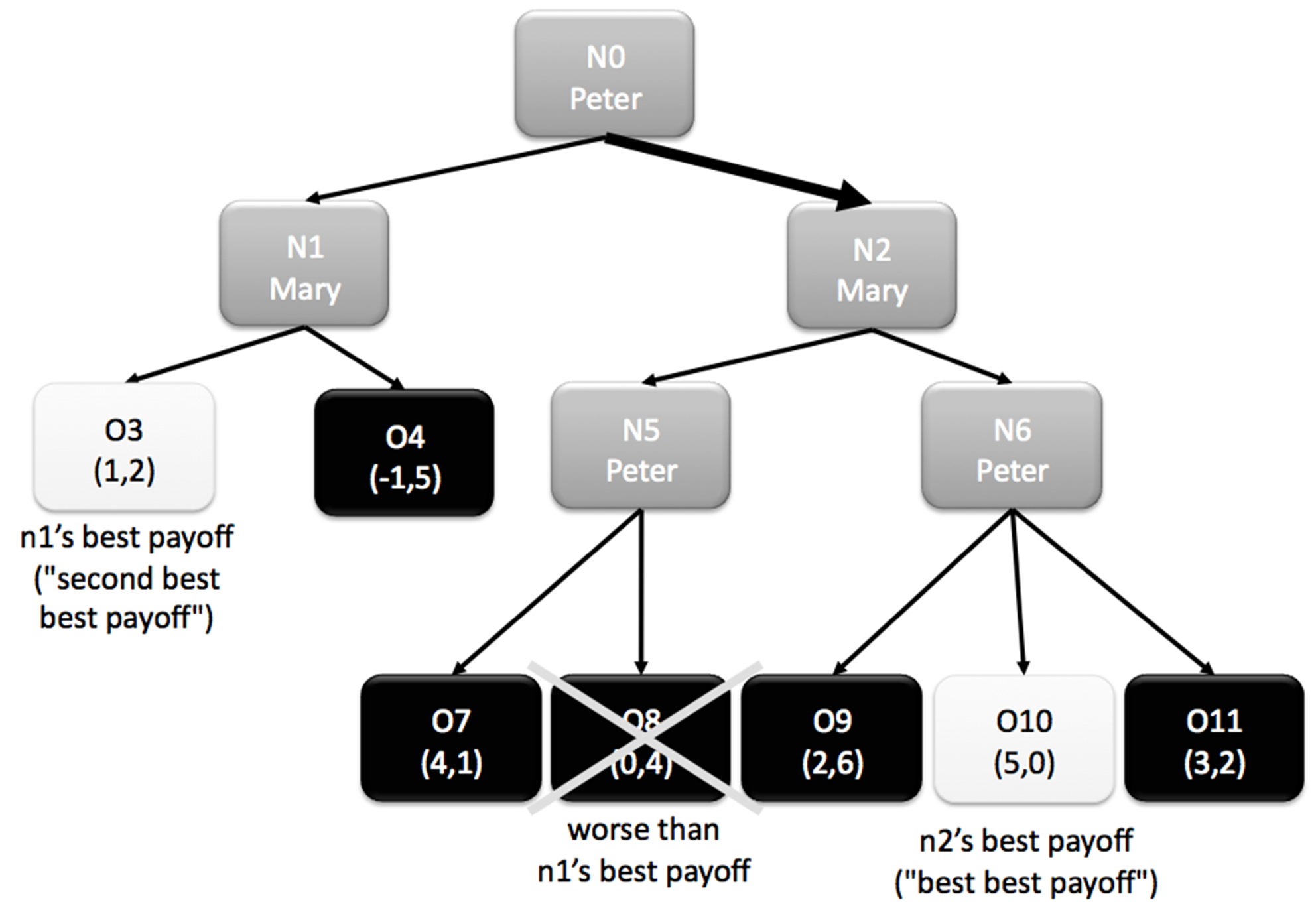
Figure 10: Illustration of the quick algorithm to determine step $2$ in Game $\Gamma$.

Therefore the preemption structure analysis indeed leads to the same results as the original definition, and it is a powerful tool which provides us with two algorithms to compute the equilibrium.

7.2 The algorithms

In this part the reader will find two algorithms computing the PPE as presented in part 3 (see Fig. 9 and 10):

- the general algorithm determines completely the Newcombian structure leading to each current player’s move. It has been directly derived from the proof of existence in Proposition 3, so that this proof is a proof of correctness for the algorithm.

- the quick algorithm calculates directly the set of remaining outcomes at each current player’s move by choosing the branch with the best outcome and eliminating all outcomes below some minimum level. This algorithm has been directly derived from the proof of uniqueness in Proposition 3, so that this proof is also a proof of correctness for the algorithm.

Both algorithms run in polynomial time with respect to the size of the tree.

7.2.1 General algorithm

This algorithm computes explicitly all intermediate discardings. It runs in $O(n^{3}d)$ where $n$ is the number of nodes and leaves in the tree and $d$ its depth.

The equilibrium path is called $(c_{i})_{i=1..d}$.

The algorithm is initialized with:

$c_{1}=n_{0}$ (the root)

$I_{1}=\{$all outcomes of the game$\}$

Then a finite induction on $i$ gives all $(c_{i})_{i=1..d}$ and all $(I_{i})_{i=1..d}$:

at each step $i$, a finite induction on $k$ gives a series of Newcombian States:

$$\{\widehat{\eta}_{(1)}^{(i)}\}\quad=\quad\arg\max_{\begin{array}[]{c}\scriptstyle\widehat{\eta}\\ \scriptstyle\mathrm{order}\left(\widehat{\eta}\right)=1\end{array}}\min_{o\in T_{i}(\widehat{\eta})}\qquad\mathbf{{payoff}}_{i}(o)$$

$$\{\widehat{\eta}_{(k+1)}^{(i)}\}\quad=\quad\arg\max_{\begin{array}[]{c}\scriptstyle\widehat{\eta}\\ \scriptstyle\widehat{\eta}=\widehat{(n,\eta_{(k)}^{(i)})}\\ \scriptstyle n\in F(c_{i-1})\backslash\{\widehat{\eta}_{(k)1}^{(i)}\}\\ \scriptstyle T_{i}(\widehat{\eta})\neq\emptyset\end{array}}\min_{o\in T_{i}(\widehat{\eta})}\qquad\mathbf{{payoff}_{i}(o)}$$

and stops at some k, giving $\widehat{\eta}_{(k)}^{(i)}=\widehat{\eta}^{(i)}$

Then

• the current player’s move is $c_{i}=\textbf{pure}(\widehat{\eta}^{(i)})$

• the remaining outcomes are $I_{i}=T_{i}(\widehat{\eta}^{(i)})$

The induction ends when the path reaches an outcome:

$$I_{d}=\{c_{d}\}$$

7.2.2 Quick algorithm

This algorithm calculates the equilibrium path without using the preemption structure. It runs in $O(nd)$ where $n$ is the number of nodes and leaves in the tree and $d$ its depth.

o $\leftarrow$ the root of the tree

While(o is not an outcome)

p $\leftarrow$ current player at node o

s $\leftarrow$ the subtree starting at an offspring of o

with the maximum payoff for player p

If(there are other subtrees than s)

M $\leftarrow$ player p’s maximum payoff in the other subtrees than s

Eliminate all other subtrees than s

Discard in s all outcomes with a payoff lower than M for player p

Clean the tree (remove all interrupted paths)

o $\leftarrow$ the root of s

Return o

Example 20

An example of application of this algorithm at the root is shown on Fig. 10. Peter’s highest payoff is at the $n_{2}$-targeted outcome $o_{10}$: $5$. Among the brothers of $n_{2}$, the subtree at $n_{1}$ has the highest best payoff: $1$. We discard all $n_{2}$-targeted outcomes whose payoff with respect to Peter are lower than $1$: $o_{8}$. We get the same next move $c_{2}=n_{2}$ and the same set $I_{2}=\{o_{7},o_{9},o_{10},o_{11}\}$as by doing the full procedure at step 2 (Fig. 9)

8 Annex - Proofs of Lemmas, Theorems and Propositions

Proof

(Lemma 1) We prove each of the three points:

1. The outcome in $I_{i-1}$ with the highest payoff for the current player $p_{c_{i-1}}$:

$$\quad\arg\max_{o\in I_{i-1}}a_{o}^{p_{c_{i-1}}}$$

cannot be discarded by a Newcombian State $\eta$. Its payoff would namely have to be lower than the worst outcome of a non-empty subset $T_{i}(\eta)$ of $I_{i-1}$, which is in contradiction with its definition.

2. Let us suppose that $I_{i}$ contains at least two outcomes descending from two different offsprings of $c_{i-1}$.

Let $o_{m}$ be the worst outcome for $p_{c_{i-1}}$ in $I_{i}$ and $f_{m}$ its ancestor among the offsprings of $c_{i-1}$. We will show that $o_{m}$ should have been discarded and so cannot be in $I_{i}$.

By assumption, there is another offspring $f_{p}\neq f_{m}$ of $c_{i-1}$, with at least one outcome which has not been discarded - let $o_{p}$ be the worst one of those, and $(f_{p},\eta)$ a Newcombian State. Because $o_{p}$ is not discarded, $o_{p}\in T_{i}(f_{p},\eta)$. By definition of $o_{m}$ and because of the strict preference between two outcomes, $o_{m}$ is strictly worse than $o_{p}$ (which is the worst outcome in $T_{i}(f_{p},\eta)$), thus is preempted by $(f_{p},\eta)$.

This is in contradiction with the fact that $o_{m}\in I_{i}$. $\Box$

Proof

(Theorem 3.1) The induction presented in Lemma 1 discards all outcomes but one. Furthermore, no other reasoning can discard this last outcome. The two players, having anticipated it, have no interest in modifying their choices and will play towards this outcome. $\Box$

Proof

(Theorem 3.2)

Suppose the outcome of the Perfect Prediction Equilibrium $o$ is not Pareto-optimal. Then there must be some outcome $o^{P}$, which Pareto-improves $o$:

$$a^{Peter}_{o}<a^{Peter}_{o^{P}}$$

$$a^{Mary}_{o}<a^{Mary}_{o^{P}}$$

(Both inequalities are strict because of the strict preferences).

This outcome $o^{P}$ has been discarded at some move $i$ by a Newcombian State $\eta$ of order $k$.

One of two:

- either $o\in T(\eta)$, in which case the current player’s payoff at $o$ is greater than (or equal to) $\eta$’s worst payoff

- or $o\notin T(\eta)$, but since $o$ was not discarded at that stage, the current player’s payoff at $o$ is necessarily strictly greater than $\eta$’s worst payoff

Since the current player’s payoff at $o_{p}$ is lower than $\eta$’s worst payoff, in both cases, we have contradicted the above inequalities. $\Box$

Proof

(Proposition 1) Given a payoff $x$, there is only one outcome $o$ that will give $x$ to the current player, in virtue of the assumption that all payoffs are different. If two nodes $n$ and $n^{\prime}$ in $F(c_{i-1})$ are different, then they cannot target the same outcome: $n\neq n^{\prime}\Rightarrow T_{i}(n)\cap T_{i}(n^{\prime})=\emptyset$. Hence there is a unique node $n$ in $F(c_{i-1})$ such that outcome $o$ is the descendant of node $n$.

There is only one Newcombian Class whose pure part is $n$ and whose worst payoff is $x$. This is because the Newcombian State $p$ discards all outcomes worse than the worst $p$-targeted outcome, whereas all better outcomes are not discarded. Hence the required Newcombian Class is defined by the set of $n$-targeted outcomes whose payoffs are greater than or equal to $x$. $\Box$

Proof

(Proposition 2) Discarding only depends on the worst outcome of the discarding Newcombian State. $\Box$

Proof

(Proposition 3) (Existence and uniqueness of move $\widehat{\eta}^{(i)}$)

Uniqueness: The pure part $n$ of the class $\widehat{\eta}^{(i)}$ necessarily targets the outcome with the highest payoff with respect to the current player. If not, then $\widehat{\eta}^{(i)}$ could not discard precisely this outcome with the highest payoff, which contradicts the definition of $\widehat{\eta}^{(i)}$.

Among the brothers of $n$, we call $m$ the node which has the highest best payoff. Then $\widehat{\eta}^{(i)}$’s worst payoff is the minimum of the payoffs of the $n$-targeted outcomes, which are (strictly) greater than $m$’s best payoff. A reason for it is that it is the minimum level to discard all outcomes targeted by the brothers of $n$. And it cannot be higher, since there is no other class which could have discarded the outcome relative to this value.

According to Proposition 1, $\widehat{\eta}^{(i)}$ is fully determined by its worst payoff.

Existence: let us define a procedure based on several little steps $k$, which are to be distinguished from the step $i$. With respect to step $i$, we define the best Newcombian Class of order $k$ denoted $\widehat{\eta}_{(k)}^{(i)}$ by induction on little step $k$.

Let us begin with $k=1$. The best Newcombian Class of order $1$, $\widehat{\eta}_{(1)}^{(i)}$, is the Newcombian Class of order $1$ with the highest worst payoff. This class exists, since Newcombian Classes of order $1$ are identified with nodes in $F(c_{i-1})$, which are all non-degenerate. Their worst payoffs are all distinct (see Proposition 1), so $\widehat{\eta}_{(1)}^{(i)}$ is unique.

$$\{\widehat{\eta}_{(1)}^{(i)}\}\quad=\quad\arg\max_{\begin{array}[]{c}\scriptstyle\widehat{\eta}\\ \scriptstyle\mathrm{order}\left(\widehat{\eta}\right)=1\end{array}}\min_{o\in T_{i}(\widehat{\eta})}\qquad\mathbf{{payoff}}_{i}(o)$$ (4)

Suppose now we have defined $\widehat{\eta}_{(k)}^{(i)}$ for some $k\geq 1$. We have to distinguish between two cases:

1. Either $\widehat{\eta}_{(k)}^{(i)}$ discards any outcome targeted by the brothers of its pure part $\textbf{pure}(\widehat{\eta}_{(k)}^{(i)})$, so the procedure is over and we have reached $\widehat{\eta}^{(i)}=\widehat{\eta}_{(k)}^{(i)}$.

2. Or there are still some brothers $n$ of $\textbf{pure}(\widehat{\eta}_{(k)}^{(i)})$, such that $(n,\widehat{\eta}_{(k)}^{(i)})$ is not degenerate. Then, by definition, the best Newcombian class $\widehat{\eta}_{(k+1)}^{(i)}$ of order $k+1$ will be the non-degenerate class $(n,\widehat{\eta}_{(k)}^{(i)})$ with the highest worst payoff. As for $\widehat{\eta}_{(1)}^{(i)}$, this class exists and is unique, because it is the maximum of the injective function $\mathbf{wp}$ on a finite set:

$$\{\widehat{\eta}_{(k+1)}^{(i)}\}\quad=\quad\arg\max_{\begin{array}[]{c}\scriptstyle\widehat{\eta}\\ \scriptstyle\widehat{\eta}=(n,\widehat{\eta}_{(k)}^{(i)})\\ \scriptstyle n\in F(c_{i-1})\setminus\{\textbf{pure}(\widehat{\eta}_{(k)}^{(i)})\}\\ \scriptstyle T_{i}(\widehat{\eta})\neq\emptyset\end{array}}\min_{o\in T_{i}(\widehat{\eta})}\qquad\mathbf{{payoff}_{i}(o)}$$ (5)

For each $n\in F(c_{i-1})\setminus\{\textbf{pure}(\widehat{\eta}_{(k)}^{(i)})\}$, because $(n,\widehat{\eta}_{(k)}^{(i)})$ is non-degenerate, there are some $n$-targeted outcomes which have not been discarded by $\widehat{\eta}_{(k)}^{(i)}$, i.e, $\mathbf{wp}((n,\widehat{\eta}_{(k)}^{(i)}))>\mathbf{wp}(\widehat{\eta}_{(k)}^{(i)})$. Since $\widehat{\eta}_{(k+1)}^{(i)}$ is one of these $(n,\widehat{\eta}_{(k)}^{(i)})$, $\mathbf{wp}(\widehat{\eta}_{(k+1)}^{(i)})>\mathbf{wp}(\widehat{\eta}_{(k)}^{(i)})$.

Since the set of outcomes is finite, the sequence $(\mathbf{wp}(\widehat{\eta}_{(k)}^{(i)}))_{k\geq 1}$ cannot increase indefinitely: we will necessarily reach case $1$ for some finite $k$. This shows the existence of $\widehat{\eta}^{(i)}$. $\Box$

Proof

(Proposition 4) (Equivalent definitions of $c_{i}$ and $I_{i}$)

Let us denote $c_{i}$ and $I_{i}$ as the current player’s move and the set of the not-yet-discarded outcomes as defined in Lemma 1, and let us denote $c^{\prime}_{i}$ and $I^{\prime}_{i}$ as they are suggested in Proposition 4.

In the uniqueness proof of $\widehat{\eta}^{(i)}$ we mentioned that $c^{\prime}_{i}$ necessarily targets the outcome $o$ with the highest payoff with respect to the current player. This very outcome cannot be discarded, hence $o\in I_{i}$. According to Lemma 1, all outcomes in $I_{i}$, thus $o$ as well, are the descendants of $c_{i}$. Hence $c_{i}=c^{\prime}_{i}$.

$I_{i}$ is defined as the set of all the outcomes that cannot be discarded at step $i$. First, we have $I_{i}\subset I^{\prime}_{i}$ since a non-discarded outcome at step i must be a descendant of $c_{i}$ (Lemma 1) and has to be targeted by the best Newcombian Class (because it is not discarded).

Then, we have $I^{\prime}_{i}\subset I_{i}$: all outcomes in $I^{\prime}_{i}$ cannot be discarded by anything, because the worst of them is strictly greater than the best outcome among the descendants of the brothers of $c_{i}$ (Uniqueness proof of Proposition 3).

Hence, $I_{i}=I^{\prime}_{i}$ as well. $\Box$

9 Annex - Biped Games: complete analysis

In this section, we perform a complete analysis of biped games and investigate when the Subgame Perfect Equilibrium is the same as the Perfect Prediction Equilibrium and when it is not.

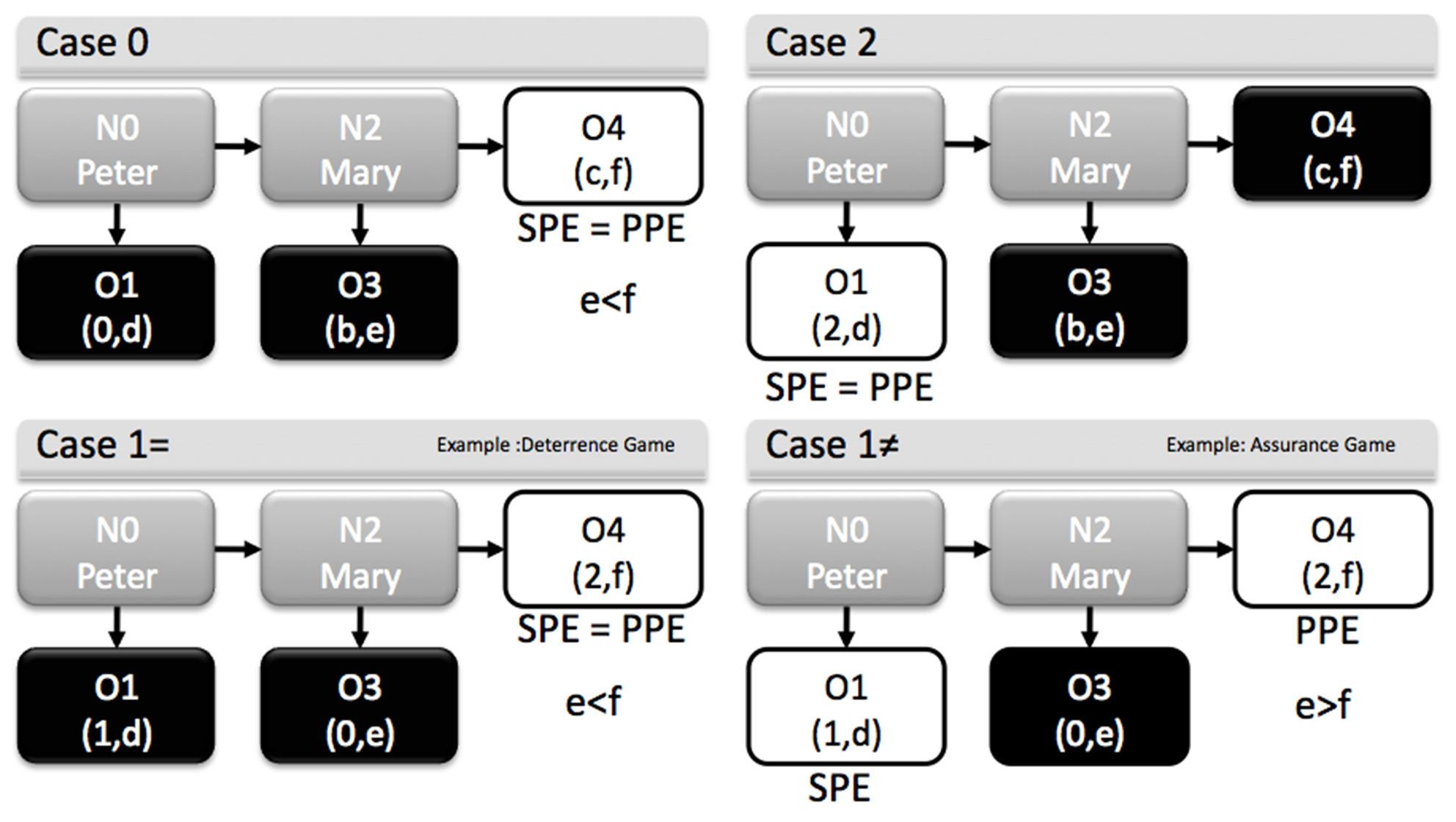
Figure 11: Biped games: the four cases

In our framework, only the order relation (preferences) between the outcomes for each player is relevant, so that without loss of generality we can assume that the payoffs are 0, 1 and 2 for each player. If we label the payoffs $(a,d)$, $(b,e)$ and $(c,f)$, we have $\frac{3!.3!}{2}=18$ different games. (We divide by two because exchanging $(b,e)$ and $(c,f)$ does not change the game). Among these 18 games, we can distinguish four cases.

• Case 0 ($a=0$, assuming $e<f$ without loss of generality - 6 different games). Both equilibria reach outcome 4. In the Subgame Perfect Equilibrium, if Mary plays at node 2, she will prefer outcome 4 which gives her f, and Peter will get c. Since $c>0$ (no indifference), Peter at node 0 will choose node 2. In the Perfect Prediction Equilibrium, Peter cannot preempt anything but outcome 1 (with node 2, since any outcome stemming from node 2 is better than outcome 1) so that Mary can choose her favorite outcome: outcome 4. This is the PPE.

• Case 1 ($a=1$, assuming $b=0$, $c=2$ without loss of generality - 6 different games). This case splits into two subcases:

  • Case 1= ($e<f$, i.e., Mary has the same preferences as Peter at node 2). Both equilibria reach outcome 4. In the Subgame Perfect Equilibrium, Mary playing at node 2 chooses outcome 4. She gets f and Peter gets 2. Peter playing at node 0 will hence choose node 2. In the Perfect Prediction Equilibrium, Peter preempts outcome 3 with outcome 0 and then plays node 2. Mary has no choice but playing outcome 4.

  • Case 1$\neq$ ($e>f$, i.e., Mary has opposite preferences to Peter at node 2). The equilibria are different. In the Subgame Perfect Equilibrium, Mary playing at node 2 chooses outcome 2. She gets e and Peter gets 0. Peter playing at node 0 will hence choose outcome 1, which is the SPE. In the Perfect Prediction Equilibrium, Peter preempts outcome 3 with outcome 0 and then plays node 2. Mary has no choice but playing outcome 4, which is the PPE.

• Case 2 ($a=2$ - 6 different games). Both equilibria reach outcome 1. In the Subgame Perfect Equilibrium, whatever Mary plays at node 2, Peter at node 0 will choose outcome 0 where he gets 2. In the Perfect Prediction Equilibrium, Peter preempts with outcome 0 all outcomes stemming from node 2 so that only outcome 0 remains. This is the PPE.

Hence, it is interesting to see that for 15 biped games out of 18, the Subgame Perfect Equilibrium and the Perfect Prediction Equilibrium are the same. Only 3 games lead to different equilibria.

For one of these three games ($d=0$, $e=2$, $f=1$), the Subgame Perfect Equilibrium encounters the Backward Induction Paradox (see Section 4.1), which is solved by the Perfect Prediction Equilibrium. For the two other games ($d=2$, $e=1$, $f=0$ and $d=1$, $e=2$, $f=0$), Peter’s preempting power is also stronger than Mary’s propensity to deviate, leading though to a PPE whose payoff is worse for Mary than at the SPE ($o_{1}$).

10 Annex - The PPE as the solution of a first-order-logic equation system

In this section, we present how a first-order-logic equation system can be built for each game, so that the PPE is the unique solution to this system. This sets up an unambiguous formal basis for defining the PPE.

The equations described in Section 10.5 induce a graph on the powerset of the outcomes: each equation contributes an edge from a set of logically impossible outcomes to a bigger set of logically impossible outcomes. Only the equations indexed on a vertex in the connected component of the empty set (i.e., all sets of logically impossible outcomes that can appear at all in any step of a reasoning) are considered for the system. A reasoning can be seen as a walk in the powerset graph induced by the first-order-logics equations, starting at the empty set. There is a unique outcome which belongs to no set in the connected component of the empty set, and this outcome is the outcome of the PPE.

10.1 Framework

The framework is the same as in this paper. $O$ is the set of all outcomes, $N$ is the set of all nodes, $F(n)$ is the set of the children of node $n$. $D(n)$ is the set of the outcomes which are descendants of node $n$. $P(n)$ is the parent of node or outcome $n$. $p_{n}$ is the player playing at node $n$. $a_{p}^{o}$ is the payoff of player $p$ at outcome $o$.

10.2 Reaction path of a tree (Second Principle)

For each tree T, we say that a path R = $(r_{i})_{0\leq i\leq l}$ starting at the root is a reaction path of $T$ if it fulfills the following conditions:

• $r_{0}$ is the root.

• For any $0<i\leq l,r_{i}\in F(r_{i-1})$

• $o\in D(r_{l})$

• (Second principle) For any $0<i\leq l$: all outcomes in $D(r_{i})$ are better than all outcomes descending from the siblings of $r_{i}$ for the player at $r_{i-1}$.

• It is maximal (there is no longer reaction path).

A non-empty tree always has exactly one reaction path (possibly simply its root). This is denoted $T\longrightarrow R$. Since a path is uniquely identified by its last node, we will also write $T\longrightarrow r_{l}$. Note that $r_{l}$ (the last node in R) is not necessarily an outcome.

10.3 Preempting reaction path of a tree to an outcome (First Principle)

For each tree T and each one of its outcomes $o$, we say that a path R = $(r_{i})_{i}$ starting at the root is a preempting reaction path of $T$ to $o$ if it fulfills the following conditions:

• $(r_{i})_{i<l}$ is a reaction path of $T$

• $r_{l}\in F(r_{l-1})$

• $o\notin D(r_{l})$

• (First principle) All outcomes in $D(r_{l})$ are better than $o$ for the player at $r_{l-1}$.

This is denoted $T\overset{o}{\rightsquigarrow}R$. Since a path is uniquely identified by its last node, we will also write $T\overset{o}{\rightsquigarrow}r_{l}$. Note that a preempting reaction path may not exist given a tree and an outcome.

10.4 Outcome Powerset Graph

More precisely, we can organize all sets of outcomes (subsets of $O$) in a graph as follows.

For each reaction path $T\setminus U\longrightarrow r$, there is an edge from $U$ to $U\bigcup(O\setminus D(r))$.

For each preempting reaction path $T\setminus U\overset{o}{\rightsquigarrow}r$, there is an edge from $U$ to $U\bigcup\{o\}$.

The semantics of an edge is: if all outcomes on the left cannot be in the solution, then all outcomes on the right cannot be either.

We call $\mathcal{U}$ the connected component of this graph containing the empty set. This corresponds to the sets of eliminated outcomes actually reachable in a reasoning.

10.5 The system of equations

Given a tree T, the system of equation is built as follows. Its unknowns are the variables $S_{n}$ for every node or outcome $n$ in the tree. $S_{n}$ is true if and only if $n$ is on the equilibrium path.

The PPE is defined as the (unique) solution of the system of equations

$$((C_{n})_{n\in(N\cup O)},(P^{1}_{e})_{e\in E_{1}},(P^{2}_{e})_{e\in E_{2}})$$

as follows.

10.5.1 The causal bridge equations

First, the equations maintaining the causal bridge are the following, for any node or outcome $n$:

$$S_{n}\Rightarrow S_{P(n)}\wedge\bigwedge_{s\in F(P(n))\setminus\{n\}}\bar{S_{s}} C_{n}$$ ()

i.e., if a node or outcome is in the solution, then its parent should be as well, and none of its siblings should be. This forces the solution to be a path on the tree.

10.5.2 The second-principle equations

Secondly, the second-principle equations are indexed on indices (U, r) in the subset $E_{2}$ of $\mathcal{U}\times O$ corresponding to reaction paths $T\setminus U\longrightarrow r$:

$$\bigwedge_{p\in U}\bar{S_{p}}\Rightarrow S_{r} P^{2}_{U,R}$$ ()

10.5.3 The first-principle (preempting) equations

Finally, the first-principle equations are indexed on indices (U, o, r) in the subset $E_{1}$ of $\mathcal{U}\times O\times O$ corresponding to preempting reaction paths $T\setminus U\overset{o}{\rightsquigarrow}r$:

$$(\bigwedge_{p\in U}\bar{S_{p}})\wedge S_{o}\Rightarrow S_{r} P^{1}_{U,o,R}$$ ()

10.6 Example for the assurance game

There are five variables here: $S_{o}=[\text{root}\in S],S_{1}=[(P,D)\in S]$, $S_{2}=[(P,C)\in S]$, $S_{3}=[(M,D)\in S]$, $S_{4}=[(M,C)\in S]$ (here we use edge labels to allow comparison with Dupuy’s original equations).

The reaction paths (and the corresponding edges in the outcome powerset graph) are:

$$\begin{array}[]{rcl}{\color[rgb]{0.7,0.2,0.2}T\longrightarrow n_{0}}&{\color[rgb]{0.7,0.2,0.2}\text{ contributing edge }}&{{\color[rgb]{0.7,0.2,0.2}\emptyset\longrightarrow\emptyset}}\\ T\setminus\{o_{1}\}\longrightarrow o_{3}&\text{ contributing edge }&\{o_{1}\}\longrightarrow\{o_{1},o_{4}\}\\ {\color[rgb]{0.7,0.2,0.2}T\setminus\{o_{3}\}\longrightarrow o_{4}}&{\color[rgb]{0.7,0.2,0.2}\text{ contributing edge }}&{\color[rgb]{0.7,0.2,0.2}\{o_{3}\}\longrightarrow\{o_{1},o_{3}\}}\\ T\setminus\{o_{4}\}\longrightarrow o_{1}&\text{ contributing edge }&\{o_{4}\}\longrightarrow\{o_{3},o_{4}\}\\ {\color[rgb]{0.7,0.2,0.2}T\setminus\{o_{1},o_{3}\}\longrightarrow o_{4}}&{\color[rgb]{0.7,0.2,0.2}\text{ contributing edge }}&{\color[rgb]{0.7,0.2,0.2}\{o_{1},o_{3}\}\longrightarrow\{o_{1},o_{3}\}}\\ T\setminus\{o_{1},o_{4}\}\longrightarrow o_{3}&\text{ contributing edge }&\{o_{3},o_{4}\}\longrightarrow\{o_{3},o_{4}\}\\ T\setminus\{o_{3},o_{4}\}\longrightarrow o_{1}&\text{ contributing edge }&\{o_{3},o_{4}\}\longrightarrow\{o_{3},o_{4}\}\\ \end{array}$$ (6)

In this example, only one preempting reaction path can be found:

$$\begin{array}[]{rcl}{\color[rgb]{0.7,0.2,0.2}T\overset{o_{3}}{\rightsquigarrow}o_{1}}&{\color[rgb]{0.7,0.2,0.2}\text{ contributing edge }}&{\color[rgb]{0.7,0.2,0.2}\emptyset\longrightarrow\{o_{3}\}}\\ \end{array}$$ (7)

The edges in the connected component of the empty set are marked in red.

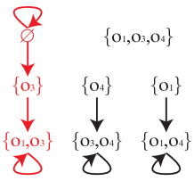
Figure 12: The Outcome Powerset Graph for the promise game

Hence, the equations are:

Causal bridge

$$S_{0}\Rightarrow\text{true} 0:C_{0}$$ ()

$$S_{1}\Rightarrow S_{0}\wedge\bar{S_{2}} 1:C_{1}$$ ()

$$S_{2}\Rightarrow S_{0}\wedge\bar{S_{1}} 2:C_{2}$$ ()

$$S_{3}\Rightarrow S_{2}\wedge\bar{S_{4}} 3:C_{3}$$ ()

$$S_{4}\Rightarrow S_{2}\wedge\bar{S_{3}} 4:C_{4}$$ ()

First Principle

$$S_{3}\Rightarrow S_{1} 5:P^{1}_{\emptyset,o_{3},o_{1})}$$ ()

Second Principle

$$\text{true}\Rightarrow S_{0} 6:P^{2}_{\emptyset,n_{0})}$$ ()

$$\bar{S_{3}}\Rightarrow S_{4} 7:P^{2}_{\{o_{3}\},o_{4})}$$ ()

$$\bar{S_{1}}\wedge\bar{S_{3}}\Rightarrow S_{4} 8:P^{2}_{\{o_{1},o_{3}\},o_{4})}$$ ()

Dupuy’s equations correspond to (5) and (7), which imply $S_{0},\bar{S_{1}},S_{2},\bar{S_{3}},S_{4}$, i.e., $\text{root}\in S$, $(P,D)\notin S$, $(P,C)\in S$, $(M,D)\notin S$ and $(M,C)\in S$ (this is our equilibrium).

Let us show this again.

From (2) and (3), one can deduce $S_{3}\Rightarrow\bar{S_{1}}$, so that because of (5), $\bar{S_{3}}$.

From (7) one deduces $S_{4}$, from (4) $S_{2}$ and from (2) or (6), $S_{0}$.

Is this a solution? With this assignment, the left part of (1), (3), (5) is false, making these implications all true, and in (0), (2), (4), (6), (7), (8), the left part is true, and the right part also, making the implications true as well.

Hence, it is proven that $S_{0},\bar{S_{1}},S_{2},\bar{S_{3}},S_{4}$ is the one and only solution of the system.

11 Annex - Link with Newcombian states

At step $i$ of the reasoning presented in Section 3, given the eliminated outcomes $I_{i-1}$, building a Newcombian state $(\eta,p)$ corresponds to the following reasoning (we abuse notations by using a node for its number).

For the first principle (preempting an outcome $o$), using equation

$$P^{1}_{(O\setminus(I_{i-1})\cup P_{i}(\text{discard}(p)),o,\eta}$$

and equation $C_{o}$ leads for $S_{o}$ to be false.

For the second principle (choosing $\eta$), using equation

$$P^{2}_{(O\setminus(I_{i-1})\cup P_{i}(\text{discard}(p)),\eta}$$

and equation $C_{\eta}$ leads for $S_{\eta}$ to be true and for $S_{o}$ to be false for each sibling $o$ of $\eta$ .

12 Annex - The special case of invertible trees

The assurance game and Take-or-Leave game are special cases of games, which are called invertible trees in Dupuy (2000). They were the starting point for defining the PPE. Their trees detain a natural chronology: at each node, the outcome below the node is in the present, whereas the previous node on the left is in the past and the next one on the right is in the future.

For these games, the procedure is rather simple and we can give a simpler version of the algorithm (but it derives from the same procedure as in the general construction). At each node, starting from the root, the current player compares the present outcome with the outcomes in the future:

1. if the present outcome is better than all outcomes in the future, the procedure stops: the PPE outcome is the present one (the future outcomes are all preempted by the present Take-move)

2. if all outcomes in the future are better than the present one, then the player Leaves (the present outcome is preempted by the Leave-move)

3. if some outcomes in the future are worse and some better than the present outcome, then first all worse outcomes in the future are preempted by the present Take-move, and then the present outcome is discarded like in point 2.

References

- Aumann (1995) Aumann RY (1995) Backward induction and common knowledge of rationality. Games and Economic Behavior 8:6–19
- Baltag et al (2009) Baltag A, Smets S, Zvesper J (2009) Keep “hoping” for rationality: a solution to the backward induction paradox. Synthese 169:301–333, URL http://dx.doi.org/10.1007/s11229-009-9559-z, 10.1007/s11229-009-9559-z
- Banks and Sobel (1987) Banks J, Sobel J (1987) Equilibrium Selection in Signaling Games. Econometrica 55:647–661
- Binmore (1996) Binmore K (1996) A note on backward induction. Games and Economic Behavior 17:135–137
- Binmore (1997) Binmore K (1997) Rationality and backward induction. Journal of Economic Methodology 4: 1:23–41
- Cho and Kreps (1987) Cho IK, Kreps D (1987) Signalling Games and Stable Equilibria. Econometrica 76:117–136
- Dupuy (2000) Dupuy JP (2000) Philosophical Foundations of a New Concept of Equilibrium in the Social Sciences: Projected Equilibrium. Philosophical Studies 100:323–356
- Gardner (1973) Gardner M (1973) Free Will Revisited, With a Mind-Bending Prediction Paradox by William Newcomb. Scientific American 229
- Govindan and Wilson (2008) Govindan S, Wilson R (2008) On Forward Induction. Econometrica 50
- Halpern (2001) Halpern JY (2001) Substantive rationality and backward induction. Games and Economic Behavior 37(2):425 – 435, DOI DOI: 10.1006/game.2000.0838, URL http://www.sciencedirect.com/science/article/pii/S0899825600908388
- Hofstadter (1983) Hofstadter D (1983) Dilemmas for Superrational Thinkers, Leading Up to a Luring Lottery. Scientific American
- Kreps and Wilson (1982) Kreps D, Wilson R (1982) Sequential Equilibria. Econometrica 50:863–894
- Kreps (2009) Kreps DM (2009) Comments on Dupré, Dupuy, and Bender. Occasion: Interdisciplinary Studies in the Humanities 1 1 http://occasion.stanford.edu/node/15
- Nash (1951) Nash J (1951) Non-cooperative Games. Annals of Mathematics 54:286 – 295
- Pettit and Sugden (1989) Pettit P, Sugden R (1989) The backward induction paradox. The Journal of Philosophy 86(4):169–182
- Reny (1992) Reny PJ (1992) Rationality in Extensive-Form Games. Journal of Economic Perspectives 6, 4:103–118
- Selten (1965) Selten R (1965) Spieltheoretische Behandlung eines Oligopolmodells mit Nachfrageträgheit [An oligopoly model with demand inertia]. Zeitschrift für die Gesamte Staatswissenschaft 121
- Shiffrin et al (2009) Shiffrin R, Lee M, Zhang S (2009) Rational Games - ‘Rational’ stable and unique solutions for multiplayer sequential games. Tech. rep., Indiana University
- Stalnaker (1998) Stalnaker R (1998) Belief revision in games: forward and backward induction. Mathematical Social Sciences 36(1):31 – 56, DOI DOI: 10.1016/S0165-4896(98)00007-9, URL http://www.sciencedirect.com/science/article/pii/S0165489698000079
- Wolpert and Benford (2013) Wolpert D, Benford G (2013) The lesson of newcomb’s paradox. Synthese 190(9):1637–1646, DOI 10.1007/s11229-011-9899-3, URL http://dx.doi.org/10.1007/s11229-011-9899-3