Boundary Conditions for Free Interfaces with the Lattice Boltzmann Method

Abstract

In this paper we analyze the boundary treatment of the lattice Boltzmann method (LBM) for simulating 3D flows with free surfaces. The widely used free surface boundary condition of Körner et al. (2005) is shown to be first order accurate. The article presents a new free surface boundary scheme that is suitable for second order accurate simulations based on the LBM. The new method takes into account the free surface position and its orientation with respect to the computational lattice. Numerical experiments confirm the theoretical findings and illustrate the different behavior of the original method and the new method.

1 Introduction

1.1 Motivation

Since its early existence, the lattice Boltzmann method has been applied in simulations of multi-phase flow phenomena (Benzi et al., 1992; Chen and Doolen, 1998; Aidun and Clausen, 2010). For the major part, these efforts have been based on diffusive interface theory (Do-Quang et al., 2000; Nourgaliev et al., 2003). The free surface lattice Boltzmann method (FSLBM) (Körner et al., 2005), instead, is based on the non-diffusive volume of fluid (VOF) approach (Hirt and Shannon, 1968; Scardovelli and Zaleski, 1999), to track the motion of the interface and to impose a free boundary condition locally. The dynamics of the gas phase is neglected and a single-phase free boundary problem is solved instead of a two-phase flow problem. The method has been used successfully in the simulation of liquid-gas flows of high viscosity and density ratio. Examples can be found in N. Thürey (2004, 2006); Xing et al. (2007b, a); Janßen (2010); Janssen et al. (2010); Attar and Körner (2011); Donath et al. (2010); Anderl et al. (2014); Ammer et al. (2014), and in Bogner and Rüde (2013); Svec et al. (2012) for complex liquid-gas-solid flows. However, no theoretical analysis of the FSLBM is currently available. Hence, the continued success in numerous applications motivates the interest in developing a better theoretical foundation of the method. In this paper we present a detailed analysis of the free surface boundary condition as it is used in the papers cited above. The analysis of lattice Boltzmann boundary schemes is mainly due to the works of Ginzburg (Ginzburg and d’Humieres, 2003; Ginzburg et al., 2008; Ginzbourg and Adler, 1994) and Junk (Junk and Yang, 2005a, b). Here, we use a Chapman-Enskog ansatz similar to Ginzburg et al. (2008), to analyze the free surface boundary treatment. We show that the original FSLBM boundary condition, referred to as FSK - rule later on, is of first order in spatial accuracy. We then proceed to propose a second order accurate free surface boundary condition as a possible improvement. The new method is based on linear interpolation (FSL - rule) and can be analyzed by the same techniques mentioned above.

The considered numerical scheme including the free surface treatment is introduced in Sec. 2. The analytic results, including the construction of the new FSL - scheme, can be found in Sec. 3. We present various numerical experiments in Sec. 4 that confirm the predicted behavior. Further discussion and outlook can be found in Sec. 5.

1.2 Liquid Interfaces and Free Boundaries

In this paragraph we introduce the model equations of a free surface. Let here $\mu=\rho\nu$ denote the dynamic viscosity of the liquid. The boundary condition at a free interface with local unit normal $\mathbf{n}$ is given by

$$(P-P_{b}+\sigma\kappa)n_{\alpha}=2\nu S_{\alpha\beta}n_{\beta},$$ (1)

where $P$ and $S_{\alpha\beta}=\frac{1}{2}\left(\partial_{\alpha}j_{\beta}+\partial_{\beta}j_{\alpha}\right)$ are the local pressure and shear rate tensor of the liquid, and $P_{b}$ is the surrounding pressure exerted on the free boundary. The term $\sigma\kappa$ expresses the usual pressure jump due to surface tension. Let $\mathbf{\tau}$ be a unit vector tangential to the interface. Projecting Eq. (1) first on $\mathbf{n}$, and second, on $\mathbf{\tau}$ yields the conditions

$$P-P_{b}+\sigma\kappa =2\nu\left(\partial_{n}j_{n}\right),$$ (2a)

$$0 =\partial_{\tau}j_{n}+\partial_{n}j_{\tau},$$ (2b)

for the normal and tangential viscous stresses, respectively. Here, $\partial_{n}$ and $\partial_{\tau}$ are the directional derivatives along $\mathbf{n}$ and $\mathbf{\tau}$, respectively, while $j_{n}=n_{\alpha}j_{\alpha}$ and $j_{\tau}=\tau_{\alpha}j_{\alpha}$.

The remaining part of this paper deals with the construction of lattice Boltzmann boundary rules, satisfying the above equations. The FSLBM according to Körner et al. (2005) uses a “link-wise” construction, as described in Ginzburg and d’Humieres (2003); Ginzburg et al. (2008) for various Dirichlet- and mixed-type boundary conditions. We follow these works with our notation, such that the new boundary rules can be easily related to the “multi-reflection” context from the same authors. We remark, however, that there exist alternative, non - “link-wise” techniques to model free surface boundary conditions (Ginzburg and Steiner, 2003), which are not considered in this article.

2 Numerical Method

In this work, we will develop the FSLBM based on a two-relaxation-time (TRT) collision operator. This collision operator uses separate relaxation times for even and odd parts of the distribution function. This is particularly important when working with boundary conditions. A generalization to other collision operators is possible, but will not change the convergence orders. The widespread single-relaxation-time (SRT) collision model, also known as lattice BGK model (Qian et al., 1992), is a special case of the TRT model, in which both relaxation times are chosen equal. Hence, the results obtained in the analysis of Sec. 3 can be transferred directly to the SRT model.

2.1 Hydrodynamic TRT-model

We assume a lattice Boltzmann equation (Benzi et al., 1992; Chen and Doolen, 1998; Aidun and Clausen, 2010) with two relaxation times according to Ginzburg et al. (2008); Ginzburg (2005). The evolution of the distribution function $\mathbf{f}=(f_{0},f_{1},..,f_{Q-1})$ on the lattice for the finite set of lattice velocities $\{\mathbf{c}_{q}\,|\,q=0,..,Q-1\}$ is then described by the equations

$$f_{q}(\mathbf{x}+\mathbf{c}_{q},t+1) =\tilde{f_{q}}(\mathbf{x},t),$$ (3a)

$$\tilde{f}_{q}(\mathbf{x},t) =f_{q}(\mathbf{x},t)+\lambda_{+}n_{q}^{+}+\lambda_{-}n_{q}^{-}+F_{q},$$ (3b)

with $n_{q}^{\pm}=f_{q}^{\pm}-e_{q}^{\pm}$. Here, Eq. (3a) is referred to as the stream step, and Eq. (3b) is the collision step, yielding the post-collision distributions $\tilde{\mathbf{f}}$. The equation has two independent relaxation times $\lambda_{+},\lambda_{-}\in(-2,0)$ for the even (symmetric) and odd (anti-symmetric) parts of the distribution function. $F_{q}$ is a source term that will be discussed later. For the discrete range of values $q\in\{0,..,Q-1\}$, the opposite index $\bar{q}$ is defined by the equation $\mathbf{c}_{q}=-\mathbf{c}_{\bar{q}}$ and thus,

$$f_{q}^{+}=\frac{1}{2}(f_{q}+f_{\bar{q}}),\;\text{ and }\;f_{q}^{-}=\frac{1}{2}(f_{q}-f_{\bar{q}}),$$ (4)

respectively. The equilibrium function $\mathbf{f}^{eq}=\mathbf{e}^{+}+\mathbf{e}^{-}$ is of polynomial type with even part

$$e_{q}^{+}(\rho,\mathbf{u})=\frac{w_{q}}{c_{s}^{2}}\Pi_{q},$$ (5)

where $\Pi_{q}=P+N_{q}$, with pressure $P$ and the non-linear contribution

$$N_{q}=\frac{1}{2}\rho_{0}u_{\alpha}u_{\beta}\left(\frac{c_{q,\alpha}c_{q,\beta}}{c_{s}^{2}}-\delta_{\alpha\beta}\right),$$ (6)

and odd equilibrium component

$$e_{q}^{-}(\rho,\mathbf{u}^{eq})=\frac{w_{q}}{c_{s}^{2}}\rho_{0}c_{q,\alpha}u^{eq}_{\alpha}.$$ (7)

Hereby, the pressure is defined by $P=c_{s}^{2}\rho$. The popular “compressible” form used in Qian et al. (1992) is obtained if one sets $\rho_{0}=\rho$. For $\rho_{0}=1$, the “incompressible” equilibrium of He and Luo (1997) is obtained. The lattice weights $w_{q}=w_{|\mathbf{c}_{q}|}$ are chosen as in Qian et al. (1992), with $c_{s}=1/\sqrt{3}$ as the corresponding lattice speed of sound. The non-linear part $N_{q}$ can be dropped for the simulation of Stokes-flow. Macroscopic quantities are defined as moments of $\mathbf{f}$. In particular, the moments of zeroth and first order,

$$\rho=\frac{1}{c_{s}^{2}}P =\sum_{q}f_{q},$$ (8)

$$\rho_{0}\mathbf{U}=\rho_{0}\mathbf{u}-\frac{\mathbf{F}}{2} =\sum_{q}\mathbf{c}_{q}f_{q},$$ (9)

define the pressure $P$ and fluid velocity $\mathbf{u}$. The shift in the fluid momentum by $\mathbf{F}/{2}$ is necessary if external forces such as gravitation are included in simulations (cf. Buick and Greated, 2000; Ginzburg et al., 2008). For the latter, one can either make use of additional force terms $F_{q}$ as in Guo et al. (2002); Buick and Greated (2000) and set $\mathbf{u}^{eq}=\mathbf{U}$, or equivalently work without the source term $F_{q}$ and use $\mathbf{u}^{eq}=\mathbf{U}-\mathbf{F}/{\lambda_{-}}$ instead. The latter simplifies the analysis (Ginzburg et al., 2008) and is adopted in the following. The fluid momentum is $\mathbf{j}=\rho_{0}\mathbf{u}$. The lattice viscosity of the model is related to the symmetric relaxation time, via

$$\nu=-\frac{1}{3}(\frac{1}{\lambda_{+}}+\frac{1}{2}).$$ (10)

2.2 Boundary Conditions

The node positions $\mathbf{x}$ are restricted to a discrete subset (lattice) of nodes within a bounded domain $\Omega\subset\mathbb{R}^{n}$.

Figure 1: Schematic view of boundary node $\mathbf{x}_{b}\in\Omega(t)$ and boundary intersection point $\mathbf{x}_{w}\in\partial\Omega(t)$ along a lattice link $\mathbf{c}_{q}$.

A node $\mathbf{x}$ is called boundary node, if the set of boundary links, $L_{b}(\mathbf{x}):=\{q\,|\,\mathbf{x}+\mathbf{c}_{q}\notin\Omega\}$, is nonempty (cf. Fig. 1). If $\mathbf{x}_{b}$ is a boundary node, then for each $q\in L_{b}(\mathbf{x}_{b})$, there is an intersection $\mathbf{x}_{w}=\mathbf{x}_{b}+\delta\mathbf{c}_{q}\in\partial\Omega$ with $0\leq\delta\leq 1$. The value $f_{\bar{q}}(\mathbf{x},t+1)$ then cannot be computed from Eq.s (3a-3b), and must be given in the form of a closure relation. For this paper we consider linear link-wise closure relations that take the general form

$$f_{\bar{q}}(\mathbf{x}_{b},t+1)=a_{0}\tilde{f}_{q}(\mathbf{x}_{b},t)+\bar{a}_{0}\tilde{f}_{\bar{q}}(\mathbf{x}_{b},t)+a_{1}\tilde{f}_{q}(\mathbf{x}_{b}-\mathbf{c}_{q},t)\\ +f_{q}^{p.c.}(\mathbf{x}_{b},t)+f^{b}_{q}(\mathbf{x}_{w},t).$$ (11)

This can be categorized as a linear multi-reflection closure rule (Ginzburg and d’Humieres, 2003; Ginzburg et al., 2008), with $\kappa_{1}=a_{0}$, $\bar{\kappa}_{-1}=\bar{a}_{0}$, $\kappa_{0}=a_{1}$, and $\kappa_{-1}=\kappa_{-2}=0$ when using the notation of the respective articles. $f_{q}^{p.c}$ is a term depending on the local non-equilibrium component $n_{q}(\mathbf{x}_{b},t)$, and $f^{b}_{q}(\mathbf{x}_{w},t)$ depends on the (macroscopic) boundary values at the wall point $\mathbf{x}_{w}$. For Dirichlet-type boundary conditions on the pressure or the momentum, respectively, this term takes the form

$$f^{b}_{q}=\alpha_{+}e_{q}^{+}(\rho_{b},\mathbf{u}_{b})+\alpha_{-}e_{q}^{-}(\rho_{b},\mathbf{u}_{b}),$$ (12)

where the $\alpha_{\pm}$ are linear combinations of the coefficients $a_{0}$, $\bar{a}_{0}$, $a_{1}$, depending on the specific boundary condition.

2.3 Free Surface Lattice Boltzmann Method

For the FSLBM according to Körner et al. (2005), the lattice Boltzmann equation scheme described above is extended by a volume-of-fluid indicator function $\varphi(\mathbf{x},t)\in[0,1]$ (Hirt and Nichols, 1981; Scardovelli and Zaleski, 1999). This function is defined as the volume fraction of liquid within the cubic unit cell centered around the lattice node at $\mathbf{x}$, thus giving an implicit description of the free surface between liquid and gas. For dynamic simulations the indicator function $\varphi$ must be advected after each time step. It represents a boundary for the hydrodynamic simulation, and its closure relation as given in Körner et al. (2005) reads

$$f_{\bar{q}}(\mathbf{x}_{b},t+1)=-\tilde{f}_{q}(\mathbf{x}_{b},t)+2\cdot e_{q}^{+}(\rho_{b},\mathbf{u}_{b}),$$ (13)

where $P_{b}=c_{s}^{2}\rho_{b}$ is the boundary value for the pressure at the free surface, and $\mathbf{u}_{b}$ is the velocity of the interface and must be extrapolated to the boundary from the nodes. The lattice Boltzmann domain $\Omega(t)$ is thus limited to nodes $\mathbf{x}$ with $\varphi(\mathbf{x},t)>0$. Eq. (13) is applied at interface nodes $\mathbf{x}_{b}$ for all links $q$ that are connected to inactive gas nodes with $\varphi(\mathbf{x}_{b}+\mathbf{c}_{q},t)=0$. Active lattice Boltzmann nodes in $\Omega(t)$ are also called liquid nodes.

Surface tension can be directly incorporated in the FSLBM by including also the Laplace pressure term $\sigma\kappa$ in Eq. (13) in place of $P_{b}$. As other interface capturing methods, this requires a local approximation of the interface curvature $\kappa$ (Scardovelli and Zaleski, 1999; Fuster et al., 2009).

3 Free surface Boundary Conditions

3.1 Chapman-Enskog Analysis

We apply the Chapman-Enskog ansatz of Ginzburg et al. (2008) for incompressible flow. Based on diffusive time scaling (Junk and Yang, 2005a), the time-derivatives of the first order in the expansion parameter $\epsilon$ are dropped and one seeks solutions to the system of Eq.s (3a-3b) with the scaled space and time step satisfying $\Delta x^{2}=\Delta t=\mathcal{O}(\epsilon^{2})$. For brevity, we introduce $\partial_{q}:=c_{q,\alpha}\partial_{\alpha}$, $j_{q}:=c_{q,\alpha}j_{\alpha}$. Then, the non-equilibrium solution up to the third order, split into even and odd parts, for constant external forcing reads

$$n_{q}^{\pm}=\frac{1}{\lambda_{\pm}}\left[\partial_{q}(e_{q}^{\mp}-\Lambda_{\mp}\partial_{q}e_{q}^{\pm})+\partial_{t}e_{q}^{\pm}\right]+\mathcal{O}(\epsilon^{3}),$$ (14)

where the coefficients $\Lambda_{\mp}$ are defined as

$$\Lambda_{\pm}=-(\frac{1}{2}+\frac{1}{\lambda_{\pm}}).$$ (15)

We further define the product $\Lambda:=\Lambda_{+}\Lambda_{-}$, which is useful to characterize the parametrization of the model. Substituting the polynomial equilibrium, Eq.s (5-7) and considering only constant external forcing, we can directly express $n_{q}$ in terms of macroscopic variables by

$$n_{q}^{+} =\frac{1}{\lambda_{+}}\frac{w_{q}}{c_{s}^{2}}\left[\partial_{q}\left(j_{q}-\Lambda_{-}\partial_{q}\Pi_{q}\right)+\partial_{t}\Pi_{q}\right],$$ (16a)

$$n_{q}^{-} =\frac{1}{\lambda_{-}}\frac{w_{q}}{c_{s}^{2}}\left[\partial_{q}(\Pi_{q}-\Lambda_{+}\partial_{q}j_{q})+\partial_{t}j_{q}\right].$$ (16b)

The approximate solution based on Eq. (14) can be used to analyze boundary conditions, by substituting into the respective closure relation and rewriting it for the macroscopic variables in question, after Taylor-expanding all occurrences of $f_{q}$ around $(\mathbf{x}_{b},t)$. Notice that space and time derivatives are of first and second order in $\epsilon$, respectively, and only terms up to $\mathcal{O}(\epsilon^{2})$ need to be included in the analysis. Based on Eq. (14), it is possible to construct new boundary schemes by substituting into a general form like Eq. (11) and then matching the unknown coefficients to yield the desired condition for the macroscopic variables. We will apply this technique to derive a higher order free surface boundary condition in Sec. 3.4. We recall that the analysis of the present paper holds for the popular SRT collision model with only one relaxation time $\lambda_{+}=\lambda_{-}$, too, if all occurrences of the anti-symmetric relaxation time $\lambda_{-}$ are replaced with the symmetric relaxation parameter $\lambda_{+}$, that controls the viscosity (cf. Sec. 2).

3.2 Analysis of the FSLBM

The free surface boundary condition of Eq. (13) is expanded around $(\mathbf{x}_{b},t)$ on the left hand side. Substituting $f_{q}=e_{q}+n_{q}$ to split equilibrium and non-equilibrium parts of the solution, and further separating into even and odd parts, one obtains up to the order $\epsilon^{2}$,

$$\left[e_{q}^{+}-\Lambda_{+}\lambda_{+}n_{q}^{+}+\frac{\lambda_{-}}{2}n_{q}^{-}+\partial_{t}(e_{q}^{+}-e_{q}^{-})\right](\mathbf{x}_{b},t)=e_{q}^{+}(\mathbf{x}_{w}).$$ (17)

Notice, that all terms associated with the point $(\mathbf{x}_{b},t)$ have been collected on the left hand side, while on the right hand side only a boundary value term associated with intersection point $\mathbf{x}_{w}$ remains. Substituting the second order non-equilibrium solution, the left hand side of Eq. (17) results in

$$\left[\left(1+\frac{1}{2}\partial_{q}+\Lambda\partial_{q}^{2}+(1-\Lambda_{+})\partial_{t}\right)e_{q}^{+}-\left(\Lambda_{+}\partial_{q}+\frac{\Lambda_{+}}{2}\partial_{q}^{2}+\frac{1}{2}\partial_{t}\right)e_{q}^{-}\right](\mathbf{x}_{b},t).$$ (18)

Finally, using the polynomial equilibria of Eq.s (5-7), neglecting the non-linear terms and dropping all time derivatives, we obtain

$$\left[(1+\frac{1}{2}\partial_{q}+\Lambda\partial_{q}^{2})P-\Lambda_{+}(1+\frac{1}{2}\partial_{q})\partial_{q}j_{q}\right](\mathbf{x}_{b},t)=P_{b}(\mathbf{x}_{w},t).$$ (19)

Obviously, the left hand side of Eq. (19) can be interpreted as a combination of the Taylor-series approximation of the pressure $P$ and shear rate $\partial_{q}j_{q}$ at the point $\mathbf{x}_{b}+1/2\mathbf{c}_{q}$. Hence, assuming $\delta=1/2$, Eq. (19) implies a second order (third order, for $\Lambda=1/8$) accurate agreement of the pressure with boundary value $P_{b}$, combined with a second order condition of vanishing shear stress in $\mathbf{x}_{w}$. One can show analytically or by numerical experiment that in the special case of a steady parabolic force-driven tangential free-surface flow over a lattice aligned plane with no-slip boundary condition is solved without error by the FSLBM when the boundary condition of Eq. (13) is applied and if the film-thickness is an integer value such that $\delta=1/2$ (cf. also Sec. 4.3). However, if $\delta\neq 1/2$, as in most relevant cases, then the spatial accuracy for both pressure and shear drops to the first order. Also, this boundary rule fulfills Eq. (2b) only, but does not include the normal viscous stress term of Eq. (2a). We will show in Sec. 3.4 how this can be improved.

3.3 Second order boundary condition for the shear rate

Starting from Eq. (11) it is possible to construct a higher order boundary condition for pressure and shear stress. To this end, we use the local correction term

$$f_{q}^{p.c.}(\mathbf{x}_{b},t)=C\cdot n_{q}^{+}(\mathbf{x}_{b},t),$$ (20)

and a boundary value term of the form

$$f_{q}^{b}=\alpha_{+}e_{q}^{+}(\rho_{b},\mathbf{u}_{b})+D\cdot c_{q,\alpha}c_{q,\beta}S_{\alpha\beta}^{b},$$ (21)

which allows to prescribe the boundary values, $P_{b}=c_{s}^{2}\rho_{b}$ for pressure, and $S_{\alpha\beta}^{b}$ for the shear rates in $\mathbf{x}_{w}$. We use $\tilde{f}_{q}(\mathbf{x}_{b}-\mathbf{c}_{q},t)=f_{q}(\mathbf{x}_{b},t+1)\approx f_{q}(\mathbf{x}_{b},t)+\partial_{t}e_{q}(\mathbf{x}_{b},t)$, and then rewrite Eq. (11) placing all terms except the boundary value $f^{b}_{q}(\mathbf{x}_{w},t)$ on the left hand side. Using the Chapman-Enskog approximation from Eq. (14) and rearranging terms, we obtain

$$\left[\alpha_{+}e_{q}^{+}+\beta_{+}n_{q}^{+}+\alpha_{-}e_{q}^{-}+\beta_{-}n_{q}^{-}+\alpha_{+}^{t}\partial_{t}e_{q}^{+}+\alpha_{-}^{t}\partial_{t}e_{q}^{-}\right](\mathbf{x}_{b},t)=f_{q}^{b}(\mathbf{x}_{w}),$$ (22)

where

$$\alpha_{+} =1-a_{0}-\bar{a}_{0}-a_{1},$$ (23a)

$$\beta_{+} =1-(1+\lambda_{+})(a_{0}+\bar{a}_{0})-a_{1}-C,$$ (23b)

$$\alpha_{-} =\bar{a}_{0}-a_{0}-a_{1}-1,$$ (23c)

$$\beta_{-} =(1+\lambda_{-})\bar{a}_{0}-(1+\lambda_{-})a_{0}-a_{1}-1,$$ (23d)

$$\alpha_{+}^{t} =1-a_{1},$$ (23e)

$$\alpha_{-}^{t} =-(1+a_{1}).$$ (23f)

The aim of the following construction is to match these coefficients with the spatial Taylor-series around $\mathbf{x}_{b}$ up to the second order for pressure and shear rate, respectively. As the spatial derivatives of pressure and momentum are contained in the non-equilibrium functions, Eq.s (16a-16b), the system of equations follows as

$$\alpha_{-} =0,$$ (24a)

$$\beta_{-} =\alpha_{+}\delta\lambda_{-},$$ (24b)

$$\beta_{+} =-\alpha_{+}\Lambda_{+}\lambda_{+},$$ (24c)

keeping $\alpha_{+}$ as free parameter. Here, $\beta_{-}$ is chosen to fit the coefficient of the first order derivative of the pressure in $n_{q}^{-}$. $\beta_{+}$ is chosen to fit the coefficient of $\partial_{q}j_{q}$ from $n_{q}^{+}$ with the second order derivative $\partial_{q}^{2}j_{q}$ from $n_{q}^{-}$. The closure relation coefficients follow from the Eq.s (23a, 24a and 24b) as

$$a_{0} =1-\alpha_{+}(\frac{1}{2}+\delta),$$ (25a)

$$\bar{a}_{0} =1-\frac{1}{2}\alpha_{+},$$ (25b)

$$a_{1} =\delta\alpha_{+}-1,$$ (25c)

while the coefficient $$C f_{q}^{p.c}$$ in the correction term , as derived from Eq. (24c), is

$$C=\alpha_{+}\lambda_{+}(\frac{1}{2}+\delta)-2\lambda_{+}.$$ (25d)

Using now Eq. (14) to express Eq. (22) in terms of gradients of the equilibria one obtains

$$\begin{split}\alpha_{+}\left(1+\delta\partial_{q}+\Lambda\partial_{q}^{2}\right)e_{q}^{+}-\alpha_{+}\Lambda_{+}\left(1+\delta\partial_{q}\right)\partial_{q}e_{q}^{-}\\ +\left(1-a_{1}-\alpha_{+}\Lambda_{+}\right)\partial_{t}e_{q}^{+}-\left(1+a_{1}-\alpha_{+}\delta\right)\partial_{t}e_{q}^{-}=f_{q}^{b},\end{split}$$ (26)

and after substituting $a_{1}$ and $f^{b}_{q}$,

$$\begin{split}\alpha_{+}\left(1+\delta\partial_{q}+\Lambda\partial_{q}^{2}\right)e_{q}^{+}-\alpha_{+}\Lambda_{+}\left(1+\delta\partial_{q}\right)\partial_{q}e_{q}^{-}+\left(2-\alpha_{+}(\delta+\Lambda_{+})\right)\partial_{t}e_{q}^{+}\\ =\alpha_{+}e_{q}^{+}(\rho_{b},\mathbf{u}_{b})-\alpha_{+}\Lambda_{+}\frac{w_{q}}{c_{s}^{2}}c_{q,\alpha}c_{q,\beta}S_{\alpha\beta}^{b}.\end{split}$$ (27)

On the right hand side, the unknown coefficient of the boundary term, Eq. (21) is determined as $D=-\alpha_{+}\Lambda_{+}\frac{w_{q}}{c_{s}^{2}}$ to fit with the left hand side. Because the spatial approximation fits up to the second order for both pressure and shear rate, the boundary condition can be classified of second order in space for both pressure and momentum.

Since $e_{q}^{+}$ contains the non-linear terms that are often responsible for numerical instabilities, the corresponding error terms deserve special attention: the spatial error of second order $\alpha_{+}(\delta^{2}/2-\Lambda)\partial_{q}e_{q}^{+}$ is bounded and independent of the viscosity if $\Lambda$ is fixed to a constant value, which is a usual requirement for parametrizations of the TRT collision model (Ginzburg et al., 2008). If the SRT model is used, then $\Lambda=(1/2+1/\lambda_{+})^{2}$, because both relaxation times $\lambda_{+}$ and $\lambda_{-}$ are identical. Hence, one should avoid values close to zero for $\lambda_{+}$, and exclude very high lattice viscosities with the SRT model. The error in time, $\alpha_{+}(1-{2}/{\alpha_{+}}+\delta+\Lambda_{+})\partial_{t}e_{q}^{+}$ depends through $\Lambda_{+}/3=\nu$ on the lattice viscosity. However, usually one either has high Mach numbers and low viscosity (high Reynolds number regime) and hence $\Lambda_{+}\ll 1$, or a high Mach number with high viscosities (low Reynolds number regime). The second case arises typically if the LBM is used to simulate Stokes-like flow, and then the non-linear terms in $e_{q}^{+}$ do not need to be included in the equilibrium function (Ladd, 1994). Hence, in this case the momentum-dependent error in time may be eliminated.

It should be noted that the coefficients $a_{0}$, $\bar{a}_{0}$ and $a_{1}$ are the identical to the linear interpolation based pressure boundary condition “PLI” of Ginzburg et al. (2008). This is a direct consequence of the construction described above of matching the coefficients of the pressure gradients in the closure relation. The coefficients $C$ and $D$, however, are different from the PLI - rule. They are needed to obtain the $\partial_{q}j_{q}$ term in the left hand side of Eq. (27), and to define the boundary value for the shear rate in the right hand side, respectively.

3.4 Second order boundary condition for free surfaces

The boundary condition of the preceding Sec. 3.3 can be used to replace the first order free surface rule of Eq. (13). In fact, the second order version of Eq. (13) is obtained by the defining Eq.s (25a-25d) and setting $S_{\alpha\beta}^{b}=0$ as boundary value. However, for full consistency with the physical model Eq.s (2a-2b), it is necessary to control the tangential and normal shear stresses individually. Let $\{\mathbf{t}_{1},\mathbf{t}_{2},\mathbf{n}\}$ be a local orthonormal basis with $\mathbf{n}$ normal to the free boundary. Using the indices $\{\alpha^{\prime},\beta^{\prime}\}$ for the corresponding coordinate system, related to the standard coordinates by rotation $l_{\alpha\beta}$, the shear rate tensor can be expressed in the local basis via

$$\bar{S}_{\alpha^{\prime}\beta^{\prime}}=l_{\alpha\alpha^{\prime}}l_{\beta\beta^{\prime}}S_{\alpha\beta}.$$ (28)

The respective entries of the shear tensor $\bar{S}_{\alpha^{\prime}\beta^{\prime}}$ can now be set individually according to Eq.s (2a-2b), leaving the remaining components untouched. In practice, $S_{\alpha\beta}$ must be obtained by extrapolation from the bulk.

	$a_{0}$	$\bar{a}_{0}$	$a_{1}$	$\alpha_{+}$	$C$	$D$
FSK	$-1$	$0$	$0$	$2$	$0$	$-2\Lambda_{+}\frac{w_{q}}{c_{s}^{2}}$
FSL	$\frac{1}{2}-\delta$	$\frac{1}{2}$	$\delta-1$	1	$\lambda_{+}(\frac{1}{2}+\delta)-2\lambda_{+}$	$-\Lambda_{+}\frac{w_{q}}{c_{s}^{2}}$

Table 1: Coefficients of closure relation, Eq. (11) with correction term $f_{q}^{p.c.}$ from Eq. (20) and boundary value term $f_{q}^{b}$ from Eq. (21). The FSK boundary rule is first order and purely local. FSL is second order and based on linear interpolation of the PDFs.

In Tab. 1 we have collected the coefficients for all the free surface conditions considered in this paper. The FSK - rule is only first order except for a plane aligned interface at distance $\delta_{x}/2$ from the boundary nodes, and equivalent to the original FSLBM closure relation, Eq. (13), if $D=0$. The FSL-rule is the free surface condition based on the construction of Sec. 3.3. This free surface condition is of second order spatial accuracy, and fully consistent with Eq.s (2a-2b). It should be noted, that by setting $D=0$, we obtain simplified boundary conditions, consistent with Eq. (2b) only, but neglecting the normal viscous stresses in Eq. (2a). The importance of these terms has been discussed for instance in McKibben and Aidun (1995); Hirt and Shannon (1968) and depends on the respective problem. In fact, for $D=0$ all shear stress components vanish at the boundary. Numerical simulations of free surface flows often use this simplified free surface condition. In this case the $S_{\alpha\beta}^{b}$ in Eq. (21) drops out, and the condition can be implemented without the construction above and without extrapolation of $S_{\alpha\beta}$.

4 Numerical Results

All test cases presented in the following have been conducted using the TRT collision operator described in Sec. 2.1 with a $D3Q19$ lattice model. The sketch of numerical test cases for the different channel flows is depicted in Fig. 2. Hereby, the flow variables are assumed constant along the $y$-axis, and the channel is rotated by an angle $\alpha$ about the $y$-axis. The test cases have been realized using the waLBerla (Feichtinger et al., 2011; Thürey et al., 2006) framework.

Figure 2: Sketch of channel flow, rotated by angle $\alpha$ with respect to the lattice.

4.1 Transient Evolution of Plate-Driven Planar Flow

In our first validation case, we monitor the transient behavior of a planar flow with initial condition $\mathbf{u}(\mathbf{x},0)=0$. The domain is periodic in the $x$- and $y$-direction, with a free surface boundary at $z=0$ and a solid wall at $z=h$, moving in the $x$-direction with constant tangential velocity of $u_{wall}=0.001$ lattice units (Cf. Fig. 2 with $\alpha=0$). This setup has been proposed by Yin et al. (2006) with the analytic Fourier series solution,

$$\frac{u_{id}(z,t)}{u_{wall}}=1-\sum_{k=0}^{\infty}{\frac{4(-1)^{k}}{(2k+1)\pi}e^{-(2k+1)^{2}\pi^{2}\mu t/(4\rho h^{2})}\times\cos\left(\frac{(2k+1)\pi z}{2h}\right)},$$ (29)

for the validation of a free-slip boundary condition that leads in this case to the same solution as the free surface condition. For $t\gg 1$ the flow quickly develops into a uniform profile, since the free surface does not impose any friction. A dimensionless time scale $T=\mu t/(\rho h^{2})$ is introduced to facilitate the evaluation of the flow at the times $T=1/64$, $1/8$, $3/8$ and $3/4$. For the simulations, we use $\rho=1$ and $\mu=1/6$ in lattice units for channels of height $h=8$, $16$, $32$, $64$. Qualitative results are shown in Fig. 3. Note, that very similar flow profiles are obtained for both the original free surface boundary condition (FSK) and the newly proposed FSL-rule, since here the channel height is restricted to have an integer value (in lattice cells). For the quantitative evaluation, we define the error as

$$\epsilon(h,T)=\frac{1}{u_{wall}}\sqrt{\frac{1}{h}\sum_{z_{i}}(u_{x}(z_{i},T)-u_{id}(z_{i},T))^{2}},$$ (30)

where $z_{i}$ ranges over all the lattice node positions along the $z$-axis. Fig. 4 shows that both boundary conditions yield correct transient behavior and the expected second order rate of convergence is exhibited clearly. The results have been obtained with a TRT - parametrization of $\Lambda=1/4$.

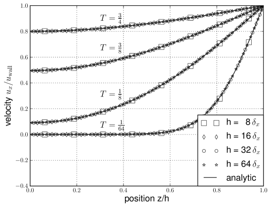
Figure 3: The velocity profile at non-dimensional times $T=1/64$, $1/8$, $3/8$. Both the original free surface boundary condition (FSK) and the new boundary condition based on linear interpolation (FSL) are very close to the analytical formula, Eq. (29).

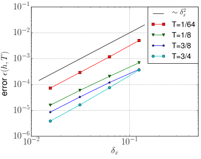
Figure 4: Grid convergence of the FSK-rule (left) and the new FSL-rule, based on linear interpolation (right) in plate driven flow at selected times. Since the channel width is an integral number, both approaches show a second order rate of convergence.

4.2 Linear Couette Flows

The analysis predicts the exact recovery of linear flow profiles when the second order boundary condition of Sec. 3.3 is used (FSL - rule with prescribed boundary value $S_{\alpha\beta}^{b}$). Here we evaluate the case of a steady flow as follows. In a cubic domain, we impose non-slip boundary conditions (bounce-back) at $z=0$, fixing the position of the first lattice nodes to the plane $z=0.5$ (Cf. Fig. 2 with $\alpha=0^{\circ}$). The shear rate condition of Sec. 3.3 is imposed at $z=h$. As a first verification experiment, a tangential shear rate is imposed by setting $S^{b}_{xz}(z=h)=0.001$. The steady Couette profile is recovered without numerical error, independent of choice of equilibrium function and film thickness $h$, in accordance with the analytical properties of the boundary condition.

Our next test case is a rotated linear film flow where bottom and top boundary planes are placed with a slope of $\Delta_{z}/\Delta_{x}=1/4$ (i.e., $\alpha\approx 14^{\circ}$ in Fig. 2). In order to realize the skew non-slip boundary, we use the CLI boundary condition of Ginzburg et al. (2008), which is a second order link-wise boundary condition similar to the one proposed by Bouzidi et al. (2001), based on linear interpolation. This boundary condition can recover steady Couette flows in arbitrary rotated channels exactly, provided that linear equilibria are employed. Applying again a tangential shear rate $\partial_{n}u_{t}=0.001$ the exact profile is recovered if the equilibrium function is restricted to the linear terms. If a non-linear equilibrium is used, a spurious Knudsen-layer appears at the boundary nodes of the skew channel where the shear rate is prescribed using Eq. (19). From the analysis, we expect this error to be of second order. A grid convergence study with fixed lattice viscosity $\nu$ and Reynolds number $Re=0.064$ is conducted, varying channel widths $h_{i}=h_{0},2h_{0},4h_{0},8h_{0}$ and imposed shear rate $\partial_{n}u_{t}=0.001,0.00025,6.25e-05,1.5625e-05$. Fig. 5 shows that the grid convergence is indeed of second order. Here and in the following sections, the relative errors are computed using either the $L^{2}$-norm,

$$L^{2}(\Phi)=\sqrt{\frac{\sum_{\mathbf{x}}(\Phi(\mathbf{x})-\Phi_{id}(\mathbf{x}))^{2}}{\sum_{\mathbf{x}}\Phi_{id}(\mathbf{x})^{2}}},$$ (31)

or the Tchebysheff norm,

$$L^{\infty}(\Phi)=\frac{\max_{\mathbf{x}}|\Phi(\mathbf{x})-\Phi_{id}(\mathbf{x})|}{\max_{\mathbf{x}}|\Phi_{id}(\mathbf{x})|},$$ (32)

where $\Phi(\mathbf{x})$ and $\Phi_{id}(\mathbf{x})$ are the respective numerical and the ideal value at the node position $\mathbf{x}$.

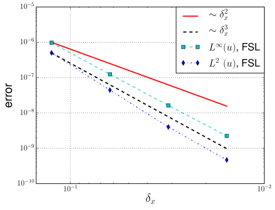
Figure 5: Second order convergence rate for linear shear flow when imposing constant shear rate on the top boundary in a skewed channel with slope $\Delta_{z}/\Delta_{x}=1/4$.

4.3 Steady Parabolic Film Flow

Force-driven slow flow of finite thickness over a planar non-slip surface admits an analytic solution that is used for validation as follows. Using a cubic domain, we impose a non-slip boundary condition at the bottom $z=0$ plane of the domain, realized using the bounce back rule. This means that the first lattice nodes are located at a distance $0.5$ from the bottom plane. At $z=h$, a free boundary is realized using the FSL boundary condition of Sec. 3.3 with $S_{\alpha\beta}^{b}=0$. We use periodic boundary conditions in the $x$ and $y$ direction. The magic parametrization $\Lambda=3/16$ for parabolic straight channel flows is used (Ginzbourg and Adler, 1994), to eliminate the error of the bounce back rule. It can be verified readily that the shear boundary condition yields the correct steady state profile without numerical error, independent of the film thickness $h$, and independent of choice of the equilibrium function. Applying additional gravity directed towards the bottom plane yields an additional linear hydrostatic pressure gradient that does not influence the solution, if the “incompressible equilibria” (He and Luo, 1997) are used. Notice, that the FSK - rule of Körner et al. (2005) is exact in this test case only if $h$ is divisible by the grid spacing, otherwise the expected accuracy is of first order $\mathcal{O}(\delta_{x})$. Fig. 6 shows that the measured error convergence for the FSK - rule given by Eq. (13) is indeed reduced to first order for $h=8.33$.

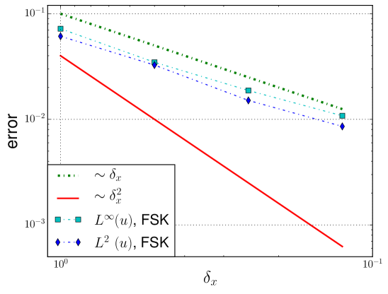
Figure 6: First order rate of convergence for a planar film flow of height $h=8.33$ with the FSK-rule. The same problem is solved exactly using the FSL-rule.

We repeat the test case with the flow direction rotated about a slope of $\Delta_{z}/\Delta_{x}=1/7$ ($\alpha\approx 8.1^{\circ}$ in Fig. 2) with respect to the lattice. The CLI boundary condition is used for the skew non-slip wall to assure a second order rate of convergence, and fix the parametrization using $\Lambda=1/4$. Similar to Couette flow, now a certain error is inevitable. Using the interpolated FSL boundary rule for the free boundary, an error convergence rate of order $\mathcal{O}(\delta_{x}^{2})$ is expected, independent of the flow direction, opposed to a first order error for the original free surface condition from Eq. (13) (FSK with $D=0$). The grid spacings are $\delta_{x}=1,0.5,0.25,0.125,0.0625$, keeping the Reynolds number constant by adjusting the accelerating force according to $g=g_{0}\times\delta_{x}^{-3}$ at a constant relaxation time $\tau=2$. Fig. 7 shows the grid convergence of the two different boundary conditions. Indeed, the proposed FSL - condition shows a second order behavior, whereas for the original FSK boundary condition the obtained rate of convergence is clearly below second order.

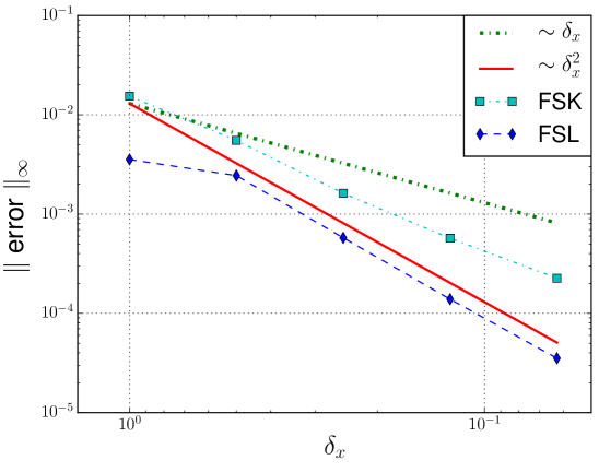
Figure 7: Comparison of the convergence behavior in a rotated planar film flow. The rate of convergence with the proposed FSL-rule is second order as predicted by the analysis. The behavior of the FSK-rule with $D=0$ is below second order.

4.4 Breaking Dam

Finally, we demonstrate the effect of the viscous stress term in the free surface condition of Eq.s (2a) and (2b) in the instationary case of a collapsing rectangular column of liquid under gravity (breaking dam). At the surge front, we have $\partial_{n}j_{n}>0$. However, the simplified boundary rule with $D=0$ forces $\partial_{n}j_{n}=0$ at the free surface, hence we expect lower acceleration of the surge front for this case. The simulated column has an initial size of $80$x$40$ lattice units. At a lattice viscosity $\nu=1/3$ and a maximal flow velocity of $0.05$ this corresponds to a Reynolds number of $Re=12$. Indeed, Fig. 8 shows that the collapse of the column is significantly slower if the terms are neglected in the boundary rule. For this experiment, we use the first order FSK rule and only first order (next-neighbor) extrapolation of $\rho$, $\mathbf{u}$ and $S_{\alpha\beta}$ to compute the boundary values. The interface tracking implementation (cf. Sec. 2.3) is directly based on the original works (Körner et al., 2005; N. Thürey, 2006).

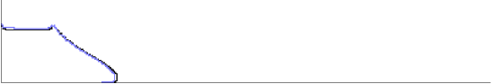
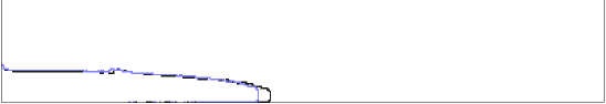
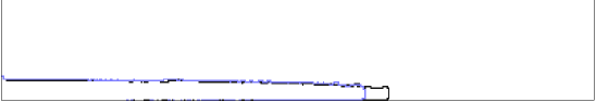
Figure 8: Simulation of a breaking dam after time step 2000, 4000, 6000, 8000. The faster surge front (black) is obtained from using the full boundary condition, while the slower front (gray blue) is obtained from the simplified boundary scheme with $D=0$ in Eq. (21).

5 Conclusion

Based on Chapman-Enskog analysis of the lattice Boltzmann equation we have described the construction of boundary conditions for free surfaces with second order spatial accuracy. In contrast to free surface models based on a discretization of the Navier-Stokes equations that need to impose boundary values for the velocity, the free surface lattice Boltzmann approach imposes the stress conditions directly on the distribution functions. Hence, the macroscopic momentum appears in the closure relation only to match the non-linear terms. The numerical experiments confirm the analytical findings, i.e., that the proposed FSL boundary scheme is of second order spatial accuracy, whereas the original FSK - model of (Körner et al., 2005) is only first order accurate. However, in order to achieve full second order accuracy, the interface position must be defined with the same order of accuracy to obtain the correct $\delta$ - values of the link intersection with the boundary. This is not possible with the interface tracking approach that is used in the original FSLBM. Hence, future implementations must make use of higher order interface reconstruction methods, or other techniques such as level sets (Osher and Fedkiw, 2001; Sethian and Smereka, 2003) to represent the free surface. Inevitably, this will introduce additional algorithmic complexity but eventually improve the accuracy (Nichols and Hirt, 1971).

For full consistency with the defining equations of a free surface, the scheme needs an approximation of the shear stress at the boundary, to impose the correct boundary values on the LBM data. In a classical dam break problem at $Re=12$, the significance of the viscous stresses at the boundary became visible. At lower viscosities this term is probably less important. It should be noted, that for under-resolved free surface simulations, it is often more accurate to employ a simplified boundary scheme, because physical viscosity and simulated viscosity do not match. For instance, Janssen et al. (2010) have reported excellent coincidence of high $Re$ - breaking dam simulations with experimental data using the original FSK - rule neglecting the viscous terms. This effect in free surface simulations has already been described in (Hirt and Shannon, 1968).

The method developed in this article can serve as basis for a second order accurate LBM - based implementation of free surface flows when combined with second order accurate interface tracking.

References

- Aidun and Clausen (2010) C. K. Aidun and J. R. Clausen. Lattice-Boltzmann method for complex flows. Annual Review of Fluid Mechanics, 42:439–472, 2010.
- Ammer et al. (2014) R. Ammer, M. Markl, U. Ljungblad, C. Körner, and U Rüde. Simulating fast electron beam melting with a parallel thermal free surface lattice boltzmann method. Computers and Mathematics with Applications, 67:318–330, 2014. doi: 10.1016/j.camwa.2013.10.001.
- Anderl et al. (2014) D. Anderl, M. Bauer, C. Rauh, U. Rüde, and A. Delgado. Numerical simulation of adsorption and bubble interaction in protein foams using a lattice boltzmann method. Food & Function, 5:755–763, 2014. doi: 10.1039/c3fo60374a.
- Attar and Körner (2011) E. Attar and C. Körner. Lattice boltzmann model for thermal free surface flows with liquid-solid phase transition. International Journal of Heat and Fluid Flow, 32(1):156–163, 2011.
- Benzi et al. (1992) R. Benzi, S. Succi, and M. Vergassola. The lattice Boltzmann equation: theory and applications. Physics Reports, 222(3):145–197, 1992.
- Bogner and Rüde (2013) S. Bogner and U. Rüde. Simulation of floating bodies with the lattice Boltzmann method. Computers and Mathematics with Applications, 65:901–913, 2013.
- Bouzidi et al. (2001) M. Bouzidi, M. Firdaouss, and P. Lallemand. Momentum transfer of a Boltzmann-lattice fluid with boundaries. Physics of Fluids, 13(11):3452, 2001.
- Buick and Greated (2000) J.M. Buick and C.A. Greated. Gravity in a lattice Boltzmann model. Physical Review E, 61(5):5307, 2000.
- Chen and Doolen (1998) S. Chen and G. D. Doolen. Lattice Boltzmann method for fluid flows. Annual Review of Fluid Mechanics, 30:329–364, 1998.
- Do-Quang et al. (2000) M. Do-Quang, E. Aurell, and M. Vergassola. An inventory of lattice Boltzmann models of multiphase flows. Technical report, Royal Institute of Technology, 2000. report no. 00:03.
- Donath et al. (2010) S. Donath, K. Mecke, S. Rabha, V. Buwa, and U. Rüde. Verification of surface tension in the parallel free surface lattice Boltzmann method in walberla. Computers & Fluids, 45(1):177–186, 2010.
- Feichtinger et al. (2011) C. Feichtinger, S. Donath, H. Köstler, J. Götz, and U. Rüde. WaLBerla: HPC software design for computational engineering simulations. Journal of Computational Science, 2(2):105–112, 2011. doi: 10.1016/j.jocs.2011.01.004.
- Fuster et al. (2009) Daniel Fuster, Gilou Agbaglah, Christophe Josserand, Stéphane Popinet, and Stéphane Zaleski. Numerical simulation of droplets, bubbles and waves: state of the art. Fluid Dynamics Research, 41(6):065001, 2009.
- Ginzbourg and Adler (1994) I. Ginzbourg and P.M. Adler. Boundary flow condition analysis for three-dimensional lattice Boltzmann model. Journal of Physics II France, 4:191–214, 1994.
- Ginzburg (2005) I. Ginzburg. Equilibrium-type and link-type lattice Boltzmann models for generic advection and anisotropic-dispersion equation. Advances in Water Resources, 28:1171–1195, 2005.
- Ginzburg and d’Humieres (2003) I. Ginzburg and D. d’Humieres. Multireflection boundary conditions for lattice Boltzmann models. Physical Review E, 68:066614–1 – 066614–29, 2003.
- Ginzburg and Steiner (2003) I. Ginzburg and K. Steiner. Lattice Boltzmann model for free-surface flow and its application to filling process in casting. Journal of Computational Physics, 185:61–99, 2003.
- Ginzburg et al. (2008) I. Ginzburg, F. Verhaeghe, and D. d’Humieres. Two-relaxation-time lattice Boltzmann scheme: About parametrization, velocity, pressure and mixed boundary conditions. Communications in Computational Physics, 3(2):427–478, 2008.
- Guo et al. (2002) Z. Guo, C. Zheng, and B. Shi. Discrete lattice effects on the forcing term in the lattice Boltzmann method. Physical Review E, 65:046308–1 – 046308–6, 2002.
- He and Luo (1997) X. He and L.-S. Luo. Lattice Boltzmann model for the incompressible Navier-Stokes equation. Journal of Statistical Physics, 88 (3/4):927–944, 1997.
- Hirt and Nichols (1981) C. W. Hirt and B. D. Nichols. Volume of fluid (vof) method for the dynamics of free boundaries. Journal of Computational Physics, 39:201–225, 1981.
- Hirt and Shannon (1968) C. W. Hirt and J.P. Shannon. Free-surface stress conditions for incompressible-flow calculations. Journal of Computational Physics, 2:403–411, 1968. doi: 0.1016/0021-9991(68)90045-4.
- Janßen (2010) C. Janßen. Kinetic approaches for the simulation of non-linear free surface flow problems in civil and environmental engineering. PhD thesis, Technische Universität Braunschweig, 2010.
- Janssen et al. (2010) C. Janssen, S. T. Grilli, and M. Krafczyk. Modelling of wave breaking and wave-structure interactions by coupling of fully nonlinear potential flow and lattice-Boltzmann models. In The International Society of Offshore and Polar Engineers (ISOPE), editors, Proceedings of the Twentieth International Offshore and Polar Engineering Conference Beijing, China, June 20-25, 2010, pages 686–693, 2010.
- Junk and Yang (2005a) M. Junk and Z. Yang. Asymptotic analysis of lattice boltzmann boundary conditions. Journal of Statistical Physics, 121 (1/2):3–35, 2005a.
- Junk and Yang (2005b) M. Junk and Z. Yang. One-point boundary condition for the lattice boltzmann method. Phys. Rev. E, 72:066701, Dec 2005b. doi: 10.1103/PhysRevE.72.066701.
- Körner et al. (2005) C. Körner, M. Thies, T. Hofmann, N. Thürey, and U. Rüde. Lattice Boltzmann model for free surface flow for modeling foaming. Journal of Statistical Physics, 121 (1/2):179–196, 2005.
- Ladd (1994) A.-J.-C. Ladd. Numerical simulations of particulate suspensions via a discretized Boltzmann equation. Part 1. Theoretical foundation. Journal of Fluid Mechanics, 271:285–309, July 1994.
- McKibben and Aidun (1995) J. F. McKibben and C. K. Aidun. Extension of the volume-of-fluid method for analysis of free surface viscous flow in an ideal gas. International Journal for Numerical Methods in Fluids, 21:1153–1170, 1995. doi: 10.1002/fld.1650211204.
- N. Thürey (2004) U. Rüde N. Thürey. Free surface lattice-Boltzmann fluid simulations with and without level sets. In Proceedings of Vision, Modeling and Visualization, pages 199–208, 2004.
- N. Thürey (2006) U. Rüde N. Thürey, K. Iglberger. Free surface flows with moving and deforming objects for LBM. In Proceedings of Vision, Modeling and Visualization, pages 193–200, 2006.
- Nichols and Hirt (1971) B. D. Nichols and C. W. Hirt. Improved free surface boundary conditions for numerical incompressible-flow calculations. Journal of Computational Physics, 8:434–448, 1971. doi: 10.1016/0021-9991(71)90022-2.
- Nourgaliev et al. (2003) R. R. Nourgaliev, T. N. Dinh, T. G. Theofanous, and D. Joseph. The lattice Boltzmann equation method: theoretical interpretation, numerics and implications. International Journal of Multiphase Flow, 29:117–169, 2003.
- Osher and Fedkiw (2001) S. Osher and R. P. Fedkiw. Level set methods: An overview and some recent results. Journal of Computational Physics, 169:463–502, 2001. doi: 10.1006/jcph.2000.6636.
- Qian et al. (1992) Y. H. Qian, D. d’Humieres, and P. Lallemand. Lattice BGK models for Navier-Stokes equations. Europhysical Letters, 17(6):479–484, 1992.
- Scardovelli and Zaleski (1999) R. Scardovelli and S. Zaleski. Direct numerical simulation of free-surface and interfacial flow. Annual Review of Fluid Mechanics, 31:567–603, 1999.
- Sethian and Smereka (2003) J. A. Sethian and P. Smereka. Level set methods for fluid interfaces. Annual Review of Fluid Mechanics, 35:341–372, 2003. doi: 10.1146/annurev.fluid.35.101101.161105.
- Svec et al. (2012) O. Svec, J. Skocek, H. Stang, M. R. Geiker, and N. Roussel. Free surface flow of a suspension of rigid particles in a non-Newtonian fluid. Journal of Non-Newtonian Fluid Mechanics, 179-180:32–42, 2012. ISSN 0377-0257.
- Thürey et al. (2006) N. Thürey, T. Pohl, U. Rüde, M. Öchsner, and C. Körner. Optimization and stabilization of LBM free surface flow simulations using adaptive parameterization. Computers & Fluids, 35(8–9):934 – 939, 2006. ISSN 0045-7930. doi: 10.1016/j.compfluid.2005.06.009. Proceedings of the First International Conference for Mesoscopic Methods in Engineering and Science.
- Xing et al. (2007a) X. Q. Xing, D. L. Butler, S. H. Ng, Z. Wang, S. Danyluk, and C. Yang. Simulation of droplet formation and coalesce using lattice Boltzmann-based single-phase model. Journal of Colloid and Interface Science, 311:609–618, 2007a.
- Xing et al. (2007b) X. Q. Xing, D. L. Butler, and C. Yang. Lattice Boltzmann-based single-phase method for free surface tracking of droplet motions. International Journal for Numerical Methods in Fluids, 53:333–351, 2007b.
- Yin et al. (2006) X. Yin, D. L. Koch, and R. Verberg. Lattice-Boltzmann method for simulating spherical bubbles with no tangential stress boundary conditions. Physical Review E, 73:026301–1 – 026301–13, 2006. doi: 10.1103/PhysRevE.73.026301.