A Two-parameter Extension of Classical Nucleation Theory

Abstract

A two-variable stochastic model for diffusion-limited nucleation is developed using a formalism derived from fluctuating hydrodynamics. The model is a direct generalization of the standard Classical Nucleation Theory. The nucleation rate and pathway are calculated in the weak-noise approximation and are shown to be in good agreement with direct numerical simulations for the weak-solution/strong-solution transition in globular proteins. We find that Classical Nucleation Theory underestimates the time needed for the formation of a critical cluster by two orders of magnitude and that this discrepancy is due to the more complex dynamics of the two variable model and not, as often is assumed, a result of errors in the estimation of the free energy barrier.

I Introduction

The process of nucleation plays an important role in chemistry, materials science and physics. For conditions of low super-saturation, characterized by large critical clusters, high energy barriers and, typically, slow (on laboratory time scales) nucleation rates, classical nucleation theory (CNT) provides an intuitively appealing framework for answering most questions of practical interestKashchiev (2000). However, modern applications in self-assembly, confined geometries and extreme conditions have shifted focus to the non-classical regime of high supersaturation, small (even nano-scale) critical clusters, low energy barriers and fast nucleation ratesDiemand et al. (2013). At the same time, and in some cases as a direct result of this shift of interest, the existence of so-called non-classical nucleation pathways have become an intense subject of investigationten Wolde and Frenkel (1997a); Vekilov (2004); Lutsko and Nicolis (2006); Sear (2012). Such pathways typically involve multi-step nucleation wherein meta-stable intermediate phases play a role. Finally, the high-supersaturation regime is also the case most easily investigated by computer simulation. All of these motivations combine to give ample practical and theoretical reason to try to extend our understanding of nucleation to the non-classical regime.

Classical nucleation theory has two important limitationsKashchiev (2000). The first is the use of the capillary approximation for the free energy of a cluster: the properties of the nucleating phase within the cluster (e.g., density, crystallinity, …) are assumed to be identical to those in the homogeneous bulk, the interface between this interior of new-phase and the bath of mother-phase is assumed to have zero width and the only dynamic property of the cluster is its size (radius, mass, etc.). For the classical regime, these are generally good approximations since interfacial widths are typically a few molecular diameters and if a cluster has radius several orders of magnitude larger than the molecular size, the effect of the finite width of the radius will be correspondingly small. However, for small clusters, consisting of perhaps only hundreds of molecules and having radius of only a few molecular diameters, nearly all molecules feel the effect of the interface and the assumptions of the capillary approximation become crude at best. Much more realistic models are available based on finite temperature Density Functional Theory (DFT)Evans (1979); Lutsko (2010) but it is then no longer possible to characterize a cluster solely by its size.

This leads to a second important limitation of CNT: since the properties of the material inside the cluster are fixed, the dynamics of cluster formation can only involve change in the size of a cluster. This is the basis for the dynamics of CNT wherein one assumes that a cluster can only grow or shrink by units of a single molecule (thus excluding, e.g., coalescence of clusters), known as the Becker-Döring modelBecker and Döring (1935). A big part of nucleation theory is then devoted to the determination of the rates of molecular attachment and detachment, see e.g. Ref. Kashchiev, 2000. Once these are specified, cluster dynamics can be viewed as a stochastic process and the rate of nucleation then determined using, e.g., Kramer’s theory of barrier crossingKramers (1940); Gardiner (2004); Hänggi et al. (1990).

Recently, a new mesoscopic description of nucleation has been developed based on fluctuating hydrodynamicsLutsko (2011a, 2012a, 2012b, 2012c). In this approach, which we will term Mesoscopic Nucleation Theory (MeNT), the fundamental quantities are the hydrodynamic fields of density, velocity and temperature. For the important case of diffusion-limited nucleation, e.g. of macromolecules in a solvent, this can be reduced to a description solely in terms of the density. The theory still requires some means for calculating the free energy of the system, but there is no conceptual limitations preventing the use of anything from the capillary approximation to very sophisticated DFT models. Assuming spherical symmetry, as is often but not always done, the density field describing a cluster can be parameterized and its evolution described solely in terms of the variation of the parametersLutsko (2012a). When the only parameter is the size of the cluster, the theory reproduces CNT (specifically, the Zeldovich equation)Lutsko and Durán-Olivencia (2013). So, this path provides an independent means of reaching the standard theory that does not require concepts such as monomer attachment/detachment rates. However, there is nothing that requires restriction to a single parameter: it is also possible to introduce multiple “order parameters” such as the density within a cluster, the width of the interface, etc. in addition to the size thus opening the door to more detailed and realistic models of cluster formation.

It should be noted that this is certainly not the first attempt to use multiple order parameters to describe nucleation. First, since as stated above, nucleation is a problem of barrier crossing and can be related to Kramer’s classic workHänggi et al. (1990), the generalization of Kramer’s results to multiple dimensions (in our language, multiple order parameters) by LangerLanger (1969); Langer and Turski (1973) and othersGardiner (2004); Hänggi et al. (1990) is of course relevant. What has previously been lacking was the detailed stochastic model to which to apply this formalism. There have been several lines of work aimed at improving the capillary description of the critical cluster, particularly the predicted excess free energy (i.e. the nucleation barrier). Notably, Reguerra, Reiss and co-workers developed the Extended Modified Liquid Drop ModelReguera and Reiss (2004) where clusters are characterized by both a mass (or number of particles) and a volume. Schweitzer, Schmelzer and co-workers introduced the Generalized Gibbs approach in which critical cluster properties such as the internal density and temperature are allowed to vary from the bulkSchmelzer and Schweitzer (1987); Schmelzer et al. (2006); Schmelzer and Abyzov (2011) with similar aims. Note that neither of these theories directly addresses the coupling of the additional parameter to the kinetics. Other developments are based on DFT-inspired calculations of the free energy of clusters. These are sometimes described in terms of order parameters and then there has been interest in using these free energy surfaces to determine nucleation pathways, typically either via application of additional constraintsGhosh and Ghosh (2011); Uline and Corti (2007); Archer and Evans (2012); Lutsko (2008a) or by gradient descent from the saddle point (e.g. the critical cluster)Lutsko (2008a, b); Philippe and Blavette (2011); Cheng et al. (2010); Qiu and Qian (2009). The constraint-based method is simply ad hoc and can lead to highly artificial behavior, see e.g. Ref.Lutsko, 2008a and, in another context, Zannetti et alZannetti et al. (2014) . The problem with the steepest-descent approaches is that gradient descent and related methods (nudged elastic band, string method, …) always requires a method of calculating distance between two points in the parameter spaceWales (2003); Lutsko (2008b). Simply having a free energy surface does not answer this requirement and all applications involve some sort of ad hoc prescription.

Mesoscopic Nucleation Theory addresses all of these issues in a self-consistent manner. Given the freedom in choosing the level of description of the free energy, the properties of the cluster can vary as freely as desired. Whatever form is chosen, it goes into a dynamical equation from which nucleation kinetics is derived. There are no a priori assumptions made about the kinetics: for example, the nucleation pathway need not even pass through the critical cluster. One obtains a complete description of the nucleation process from the formation of the initial density fluctuations through to the deterministic growth of post-critical clusters. Gradient descent plays a role in the so-called weak noise limit but one uses a measure of distance completely specified by the dynamics inherited from the fundamental, fluctuating hydrodynamics. This will be made explicit below.

The purpose of this paper is to begin the exploration of such a generalized approach, which could justifiably be viewed as multi-parameter CNT. It turns out that there are a number of conceptual problems to be solved, even given a well-defined formalism, so that attention here is limited to the very simplest case: condensation of a dense phase from a low-density phase, analogous to liquid-vapor nucleation. To be specific, we will illustrate our calculations by applying the formalism to the nucleation of a dense droplet of protein from a weak solution, a process of intrinsic interest due to its role as the first step in the non-classical crystallization of proteinsten Wolde and Frenkel (1997b); Vekilov (2004); Lutsko and Nicolis (2006); Gunton et al. (2007). Similarly, in the interest of simplicity, only one additional order parameter is considered: the density within the cluster is allowed to vary as well as its size. As will be shown, this is sufficient to lead to significant conceptual differences in the nucleation process as described by the classical one-parameter and more general two-parameter theories. We will quickly be led to construct the model so as to impose mass conservation leading to a cluster structure very similar to that of the Modified Extended Liquid Drop model mentioned above. Our primary practical conclusion is that the differences between CNT and our more complex model cannot be explained merely by the differences in the calculated free energy barriers, as is often assumed, but rather are also due to the difference in dynamics of the two theories.

In Section II we outline the theoretical framework that will be used to construct our extended description of nucleation and we show how CNT can be easily derived within this context. The next Section is devoted to the development of a two-variable model. The naive extension of CNT is shown to fail and the additional concept of mass conservation is invoked to construct a physically acceptable model. In Section IV, we apply the theory to the description of the weak-solution/dense-solution transition in globular proteins. In particular, we discuss the systematic differences observed between CNT and the two-variable theory. We summarize our conclusions in Section V.

II Theory

Our goal is the description of diffusion limited nucleation as is applicable to phase transitions in colloids and solutions of macromolecules. The prototypical problem is the nucleation of a dense phase - either a disordered, liquid-like droplet or an ordered crystalline phase - from a weak solution. However, the theory is equally applicable to the reverse - i.e. the nucleation of a low-density phase from a dense solution (the analog of the formation of a gas bubble in a one-component liquid).

The fundamental viewpoint of MeNT is that the new phase forms a cluster which is characterized by its space- and time-dependent local density (e.g. the density of the colloid or macromolecule which is equivalent to its concentration in the solution). A disordered phase has a density which is (nearly) constant while an ordered phase has a density field exhibiting molecular-scale structure. In either case, the evolution of the colloidal density is the focus of attention. Since the initial, low-concentration solution is presumed to be a metastable phase, there is an energy barrier that must be overcome for nucleation to occur and the theory must describe the thermal fluctuations which are responsible for driving the system over this barrier.

The density field is in general coupled to other fields, e.g. temperature and velocity. However, we specialize here to the case of diffusion limited nucleation as is appropriate for large molecules (or colloids) in solution. The system is, in consequence of the coupling to the bath, athermal. Furthermore, we assume over-damping which allows the velocity field to be eliminated as described in Ref. Lutsko, 2012a.

II.1 Framework

In the over-damped regime, the density field, $\rho\left(\mathbf{r}\right)$, obeys a Langevin equation of the formLutsko (2011a, 2012a)

$$\frac{d}{dt}\rho\left(\mathbf{r};t\right)=D\mathbf{\nabla}\cdot\rho\left(\mathbf{r};t\right)\mathbf{\nabla}\left(\frac{\delta\beta F\left[\rho\right]}{\delta\rho\left(\mathbf{r}\right)}\right)_{\rho\left(\mathbf{r}\right)\rightarrow\rho\left(\mathbf{r};t\right)}+\mathbf{\nabla}\cdot\varepsilon\sqrt{2D\rho\left(\mathbf{r};t\right)}\xi\left(\mathbf{r};t\right)$$ (1)

where $D$ is the low-density diffusion constant, $F\left[\rho\right]$ is a coarse-grained free energy functional, $\beta=1/k_{B}T$ is the inverse temperature and $\varepsilon$ is an artificial parameter included for explanatory purposes. The physical case always corresponds to $\varepsilon=1$. The term $\xi\left(\mathbf{r};t\right)$ is a fluctuating force that is white and delta-correlated in both space and time. The diffusion constant is related to the temperature via $D=k_{B}T/\gamma m$ where $\gamma$ characterizes the friction experienced by the large molecules due to the bath and where $m$ is the mass of the large molecules. While it is possible to work directly with the density field, here we simplify the problem by introducing a restricted set of variables. To do this, the density is represented in terms of a collection of $N$ parameters as

$$\rho\left(\mathbf{r};t\right)=f\left(\mathbf{r};x^{1}\left(t\right),x^{2}\left(t\right),...x^{N}\left(t\right)\right)\equiv\rho\left(\mathbf{r};\mathbf{x}\left(t\right)\right)$$ (2)

for some fixed functional form $f$. (The second equivalence defines a short-hand notation for this representation.) For example, to describe a dense cluster, the form of $f$ might be a sigmoidal function with the parameters being the position and width of the interface. We note that such parameters are in general constrained for physical reasons: for example, the radius and density both must be non-negative. This $N$-dimensional parameter space will be denoted $\Sigma$. For an under-saturated system, we expect that the equilibrium state will be described by a particular set of parameters corresponding to a spatially constant density and that the dynamics, in the absence of thermal fluctuations, will tend to drive any deviation from this state towards this equilibrium state. In a supersaturated system, this will be true for a certain region of parameter space - the metastable region - but there will be other parts of parameter space corresponding to super-critical clusters which will tend (in the absence of thermal fluctuations) to grow indefinitely thus converting the entire system to the new phase.

It has been shownLutsko (2012a) that the stochastic differential equation for the field gives rise to an approximate dynamics for the parameters. In the particular case of an infinite system with spherical symmetry, the parameters obey

$$\frac{dx^{i}}{dt}=-Dg^{ij}\left(\mathbf{x}\right)\frac{\partial\beta\Omega}{\partial x^{j}}+D\varepsilon^{2}A^{i}\left(\mathbf{x}\right)+\varepsilon\sqrt{2D}q_{a}^{i}\left(\mathbf{x}\right)\xi^{a}\left(t\right)$$ (3)

where the Einstein summation convention is used and this equation must be interpreted using the Ito calculusLutsko (2012a). The matrix of kinetic coefficients $g^{ij}\left(\mathbf{x}\right)$ is related to the amplitude of the noise via $g^{ij}\left(\mathbf{x}\right)=q_{a}^{i}\left(\mathbf{x}\right)q_{a}^{j}\left(\mathbf{x}\right)$. In the following, we use standard covariant notation whereby $g^{ij}$ is the inverse of the matrix $g_{ij}$ so that $g^{ij}g_{jk}=\delta_{k}^{i}$, the latter being the usual Kronecker delta function. As discussed elsewhere, the matrix $g_{ij}$ plays the role of a ”metric” in the space of parameters, $\mathbf{x}$ and this will be relevant when we discuss numerical simulation of these equations (see, e.g. Appendices D and E). For a given parameterization of the density, and in three dimensions, it (the inverse of the matrix of kinetic coefficients) is calculated as

$$g_{ij}\left(\mathbf{x}\right)=\int_{0}^{\infty}\frac{1}{4\pi r^{2}\rho\left(r;\mathbf{x}\right)}\frac{\partial m\left(r;\mathbf{x}\right)}{\partial x^{i}}\frac{\partial m\left(r;\mathbf{x}\right)}{\partial x^{j}}dr$$ (4)

where the cumulative mass density is

$$m\left(r;\mathbf{x}\right)=4\pi\int_{0}^{r}\rho\left(r^{\prime};\mathbf{x}\right)r^{\prime 2}dr^{\prime}.$$ (5)

The other quantities appearing in Eq.(3) are the grand-potential,

$$\Omega\left(\mathbf{x}\right)=F\left(\mathbf{x}\right)-\mu N\left(\mathbf{x}\right)$$ (6)

where $F\left(\mathbf{x}\right)$ is just the coarse-grained free energy, $F\left[\rho\right]$, evaluated using the model density $\rho\left(\mathbf{r};\mathbf{x}\left(t\right)\right)$ and the total number of particles is $N\left(\mathbf{x}\right)=\lim_{r\rightarrow\infty}m\left(r;\mathbf{x}\right)$. (Technically, this quantity is infinite but we can equally well work with the difference from the background which is always finite.) The noise term is white with correlations $\left\langle\xi_{i}\left(t\right)\xi_{j}\left(t^{\prime}\right)\right\rangle=\delta_{ij}\delta\left(t-t^{\prime}\right)$ and the noise amplitude is related to the metric by $q^{i}_{a}q^{j}_{b}\delta^{ab}=g^{ij}$ (e.g., see Appendix C for the explicit relation with two parameters). The final new term appearing in the SDE is the anomalous force. Before giving its form, we note that the SDE for the order parameters is not Ito-Stratonovich equivalent. When it is written in the Ito form, the anomalous force takes the form

$$A^{i}=\frac{\partial g^{ij}}{\partial x_{j}}+\frac{1}{2}g^{ij}g^{lk}\frac{\partial g_{lk}}{\partial x_{j}}+\Delta A^{i}$$ (7)

The term $\Delta A^{i}$ is given elsewhereLutsko (2012a) and will be neglected here for several reasons. First, it vanishes identically for a single order parameter and its inclusion would complicate the comparison between the one- and two-variable theories. Second, it also does not occur in the case of an infinite number of parameters, i.e. in the full hydrodynamic theory. This leads us to suspect it is an artifact of the approximations required in the derivation. Finally, the structure of the theory without this term is much nicer allowing for several important analytic results as discussed below. The effect of including it will be the subject of a later investigation.

The Fokker-Plank equation describing the probability to observe parameters $\mathbf{x}$ at time $t$, $P(\mathbf{x},t)$, follows directly from the stochastic model, Eq.(3), and is

$$\frac{\partial}{\partial t}P=-D\frac{\partial}{\partial x^{i}}\left\{-g^{ij}\left(\mathbf{x}\right)\frac{\partial\beta\Omega}{\partial x^{j}}+\varepsilon^{2}A^{i}\left(\mathbf{x}\right)-\varepsilon^{2}\frac{\partial}{\partial x^{j}}g^{ij}\right\}P$$ (8)

It is immediately apparent that the stationary probability density (valid only for under-saturated solutions) is simply

$$P\left(\mathbf{x}\right)=\mathcal{N}\sqrt{\det g\left(\mathbf{x}\right)}e^{-\beta\Omega\left(\mathbf{x}\right)}$$ (9)

where $\mathbf{x}$ is any collection of parameters (i.e. in the simplest case, it could be the radius or excess mass of the cluster), $\mathcal{N}$ is a normalization constant and $detg(\mathbf{x})$ will here and hereafter always denote the determinant of the inverse of the matrix of kinetic coefficients (i.e. of the metric).

Nucleation occurs when the system starts somewhere in the metastable region and is driven by thermal fluctuations to the stable region. We characterize the (inverse of the) nucleation rate by the mean-first passage time for the formation of a critical cluster Hänggi et al. (1990). For the one dimensional case, there is an exact expression for this quantity (discussed below), however, in the general case no such result exists. The standard resultLanger (1969); Talkner (1987); Hänggi et al. (1990); Gardiner (2004) valid in the weak noise limit is, in our language,

$$t_{mfp}=\varepsilon^{-1}\frac{\pi}{D\left|\lambda_{-}\right|}\frac{\sqrt{\left|\det\beta\Omega_{ij}^{\left(c\right)}\right|}}{\sqrt{\det g(\mathbf{x}_{c})}\left(2\pi\right)^{N/2}}\left(\int_{\Sigma_{meta}}\sqrt{\det g\left(\mathbf{x}\right)}e^{-\beta\Omega\left(\mathbf{x}\right)}d\mathbf{x}\right)e^{\beta\Omega(\mathbf{x}_{c})}$$ (10)

where $\Omega_{ij}^{\left(c\right)}$ is the Hessian of the free energy evaluated at the critical cluster $\mathbf{x}_{c}$, $\lambda_{-}$ the (sole) negative eigenvalue of $g^{ij}(\mathbf{x}_{c})\Omega_{jk}^{\left(c\right)}$ and $N$ is the number of order parameters. The critical cluster is determined as usual by $\left.\partial\Omega(\mathbf{x})/\partial x^{i}\right|_{\mathbf{x}_{c}}=0$.

II.2 A comment on covariance

It is common, in a heuristic context, to suppose that the probability of observing a cluster of mass $M$ is $P\left(M\right)\sim e^{-\beta\Delta\Omega\left(M\right)}dM$ where $\Delta\Omega\left(M\right)$ is the work of formation of the cluster or, in other contexts, to suppose that the probability to observe a cluster of radius $R$ is $\widetilde{P}\left(R\right)\sim e^{-\beta\Delta\widetilde{\Omega}\left(R\right)}dR$. Since the two quantities are related by the cluster’s density, $M=\frac{4\pi}{3}R^{3}\rho$, the work of formation in the two cases is related by $\Delta\widetilde{\Omega}\left(R\right)=\Delta\Omega\left(M\left(R\right)\right)=\Delta\Omega\left(\frac{4\pi}{3}R^{3}\rho\right)$ and the probability densities are related unambiguously by $P\left(M\right)dM=\widetilde{P}\left(R\right)dR$ or $\widetilde{P}\left(R\right)=\frac{dM}{dR}P\left(M\left(R\right)\right)=4\pi R^{2}\rho P\left(M\left(R\right)\right)$. Hence, it cannot be simultaneously be true that both probability densities are given by $e^{-\beta\Delta\Omega}$. This ambiguity is termed a lack of covariance, by which we mean that the result seems to depend on which variable we choose to start with. Nature, of course, is unambiguous and such a dilemma indicates that some element of physics is missing.

In MeNT, no such ambiguity is present. For example, in the under-saturated state, the probability density to observe a cluster described by the variables $\mathbf{x}$ is $P\left(\mathbf{x}\right)\mathbf{=}\mathcal{N}\sqrt{\det g\left(\mathbf{x}\right)}e^{-\beta\Delta\Omega\left(\mathbf{x}\right)}$. For some other set of variables, $\mathbf{y}$, related to the original variables as $\mathbf{y}(\mathbf{x})$, we get $\widetilde{P}\left(\mathbf{y}\right)\mathbf{=}\widetilde{\mathcal{N}}\sqrt{\det\widetilde{g}\left(\mathbf{y}\right)}e^{-\beta\Delta\widetilde{\Omega}\left(\mathbf{y}\right)}$ where of course $\Delta\widetilde{\Omega}\left(\mathbf{y}\right)=\Delta\Omega\left(\mathbf{x}\left(\mathbf{y}\right)\right)$. However, from the definition given above, it is immediately apparent that $\sqrt{\det\widetilde{g}\left(\mathbf{y}\right)}=\sqrt{\det g\left(\mathbf{x}\left(\mathbf{y}\right)\right)}\left|\frac{\partial\mathbf{x}}{\partial\mathbf{y}}\right|$ where the second factor is the Jacobian of the change of variables. Hence, we see that

$$\widetilde{P}\left(\mathbf{y}\right)d\mathbf{y} \mathbf{=}\widetilde{\mathcal{N}}\sqrt{\det\widetilde{g}\left(\mathbf{y}\right)}e^{-\beta\Delta\widetilde{\Omega}\left(\mathbf{y}\right)}d\mathbf{y}$$ (11)

$$=\widetilde{\mathcal{N}}\sqrt{\det g\left(\mathbf{x}\left(\mathbf{y}\right)\right)}\left|\frac{\partial\mathbf{x}}{\partial\mathbf{y}}\right|e^{-\beta\Delta\Omega\left(\mathbf{x}\left(\mathbf{y}\right)\right)}d\mathbf{y}$$

$$=\widetilde{\mathcal{N}}\sqrt{\det g\left(\mathbf{x}\left(\mathbf{y}\right)\right)}e^{-\beta\Delta\Omega\left(\mathbf{x}\left(\mathbf{y}\right)\right)}d\mathbf{x}$$

$$=P\left(\mathbf{x}\right)d\mathbf{x}$$

so that the result is independent of which set of equivalent variables one starts with. Similarly, the expression for the mean first passage time given above can also be seen to be covariant. This serves to confirm the internal consistency of the theory.

II.3 Classical Nucleation Theory

Classical Nucleation Theory (CNT) fits easily within this framework. Suppose we wish to describe the nucleation of a new phase with density (or concentration) $\rho_{0}$ in a system with initial density $\rho_{\infty}$. The notation is motivated by the idea that the density is a spatially varying field in the underlying fluctuating hydrodynamics and a cluster will have the density or the new phase, $\rho_{0}$, near the origin and that of the old phase, $\rho_{\infty}$, far away from the origin. We suppose that when the density is constant (i.e. in the bulk state) we are able to calculate the free energy per unit volume as a function of average density, $\omega\left(\rho\right)$, and the planar surface tension at coexistence, $\gamma^{(c)}$. Note that the former depends on both the temperature and the chemical potential, $\mu$ and can be expressed in terms of the Helmholtz free energy per unit volume, $f\left(\rho\right)$, as $\omega\left(\rho\right)=f\left(\rho\right)-\mu\rho$. In terms of these quantities, the excess free energy (relative to the background or mother phase) of a cluster of radius $R$ is calculated using the capillary approximation as

$$\Delta\Omega\left(R;T,\mu\right)=V\left(R\right)\left(\omega\left(\rho_{0}\right)-\omega\left(\rho_{\infty}\right)\right)+S\left(R\right)\gamma^{(c)}$$ (12)

where the $V\left(R\right)$ and $S\left(R\right)$ are the volume and surface area, respectively. The bulk densities satisfy, for fixed $\mu$ and $T$, $f^{\prime}\left(\rho_{0}\right)=\mu=f^{\prime}\left(\rho_{0}\right)$. Implicit in this model is a density profile whereby the local density as a function of distance from the center of the cluster, $\rho\left(r\right)$, is piece-wise constant having $\rho(r)=\rho_{0}$ for $r<R$ and $\rho(r)=\rho_{\infty}$for $r>R$. The radius varies with time and, as such, is the single order parameter characterizing the cluster. A simple calculation gives

$$g_{RR}=4\pi\frac{\left(\rho_{0}-\rho_{\infty}\right)^{2}}{\rho_{\infty}}R^{3},A=-\frac{3}{8\pi R^{4}}\frac{\rho_{\infty}}{\left(\rho_{\infty}-\rho_{0}\right)^{2}}$$ (13)

so that the time evolution of the radius is

$$\frac{dR}{dt}=-D\frac{\rho_{\infty}}{4\pi\left(\rho_{0}-\rho_{\infty}\right)^{2}R^{3}}\frac{\partial\beta\Omega}{\partial R}-D\frac{3}{8\pi}\frac{\rho_{\infty}}{\left(\rho_{\infty}-\rho_{0}\right)^{2}}R^{-4}+\varepsilon\sqrt{2D\frac{\rho_{\infty}}{4\pi\left(\rho_{0}-\rho_{\infty}\right)^{2}R^{3}}}\xi\left(t\right)$$ (14)

and the Fokker-Planck equation is

$$\frac{\partial}{\partial t}P=-D\frac{\rho_{\infty}}{4\pi\left(\rho_{0}-\rho_{\infty}\right)^{2}}\frac{\partial}{\partial R}\left\{-R^{-3}\frac{\partial\beta\Omega}{\partial R}-D\frac{3}{2}R^{-4}-\frac{\partial}{\partial R}R^{-3}\right\}P$$ (15)

For under saturated conditions, equilibrium is achieved in the uniform state with density $\rho_{\infty}$ and radius $R=0$. The distribution for fluctuations in cluster size is

$$P\left(R;T,\mu\right)=\mathcal{N}R^{3/2}e^{-\beta\Delta\Omega\left(R;T,\mu\right)}$$ (16)

where $\mathcal{N}$ is determined by normalization. In the limit of large clusters, the $R^{-4}$ term in Eq.(15) above can be neglected and the result is equivalent to the Zeldovich equation of CNTKashchiev (2000); Lutsko and Durán-Olivencia (2013). In this way, we see that CNT is recovered within the formalism of MeNT.

For a supersaturated system, the free energy has a minima at the metastable density $\rho_{\infty}$ with $R=0$ and at the stable density $\rho_{0}$ with $R\rightarrow\infty$. There is as well a free energy maximum at the critical radius,

$$R_{c}=\frac{2\gamma^{(c)}}{\omega\left(\rho_{\infty}\right)-\omega\left(\rho_{0}\right)}$$ (17)

with

$$\Delta\Omega\left(R_{c};T,\mu\right)=\frac{16\pi}{3}\frac{\gamma^{(c)3}}{\left(\omega\left(\rho_{\infty}\right)-\omega\left(\rho_{0}\right)\right)^{2}}.$$ (18)

In this one-dimensional case, the mean first passage time for a cluster that is initially in the metastable state to cross the nucleation barrier is Gardiner (2004)

$$t_{mfp}=D^{-1}\frac{4\pi\left(\rho_{0}-\rho_{\infty}\right)^{2}}{\rho_{\infty}}\int_{0}^{R_{c}}dR\;R^{3/2}e^{\beta\Delta\Omega\left(R\right)}\;\int_{0}^{R}dR^{\prime}R^{\prime 3/2}e^{-\beta\Delta\Omega\left(R^{\prime}\right)}\;$$ (19)

An approximate evaluation is possible by first noting that the factor $e^{\beta\Delta\Omega\left(R\right)}$ is large near $R=R_{c}$ and that the second integral is slowly varying for $R$ near $R_{c}$ since its largest contribution comes from the neighborhood of $R^{\prime}=0$. Hence, the upper limit of the second integral can be replaced by $R_{c}$ giving

$$t_{mfp}\simeq D^{-1}\frac{4\pi\left(\rho_{0}-\rho_{\infty}\right)^{2}}{\rho_{\infty}}\int_{0}^{R_{c}}dR\;R^{3/2}e^{\beta\Delta\Omega\left(R\right)}\;\int_{0}^{R_{c}}dR^{\prime}R^{\prime 3/2}e^{-\beta\Delta\Omega\left(R^{\prime}\right)}$$ (20)

Then, quadratic approximations of the free energy near the points $R=0$ and $R=R_{c}$ give the approximate evaluation

$$t_{mfp}\simeq D^{-1}\frac{4\pi\left(\rho_{0}-\rho_{\infty}\right)^{2}}{\rho_{\infty}}\left(R_{c}^{3/2}\sqrt{\frac{\pi}{2\left|\beta\Delta\Omega\left(R_{c}\right)\right|}}\right)\;\left(\left(\beta\Delta\Omega^{\prime\prime}\left(0\right)\right)^{-5/2}\frac{\pi}{2^{\frac{5}{4}}\Gamma\left(\frac{3}{4}\right)}\right)\;$$ (21)

or

$$t_{mfp}\simeq D^{-1}\frac{\left(\rho_{0}-\rho_{\infty}\right)^{3/2}}{\rho_{0}}\frac{\pi^{3/4}}{4\sqrt{2}\Gamma\left(\frac{3}{4}\right)}\left|\Delta\omega\right|^{-3/2}\gamma^{(c)-\frac{1}{4}}e^{\beta\Delta\Omega\left(R_{c}\right)}\;\;$$ (22)

It is interesting to compare these successive approximations with the general approximate result given above, Eq.(10), which here reduces to

$$t_{mfp} =\sqrt{\frac{\pi g_{RR}\left(R_{c}\right)}{2D\Delta\Omega^{\prime\prime}\left(R_{c}\right)}}\left(\int_{0}^{R_{c}}\sqrt{g_{RR}\left(R\right)}e^{-\beta\Omega\left(R\right)}dR\right)e^{\beta\Omega\left(R_{c}\right)}$$ (23)

$$=D^{-1}\frac{4\pi\left(\rho_{0}-\rho_{\infty}\right)^{2}}{\rho_{\infty}}\sqrt{\frac{\pi}{2\Delta\Omega^{\prime\prime}\left(R_{c}\right)}}R_{c}^{3/2}\left(\int_{0}^{R_{c}}R^{3/2}e^{-\beta\Omega\left(R\right)}dR\right)e^{\beta\Omega\left(R_{c}\right)}$$

This corresponds to the saddle point approximation for the first integral in Eq.(20) and an exact evaluation of the second.

III Two-parameter models

III.1 A naive extension of CNT

III.1.1 The density profile

Our goal is to generalize the CNT description of nucleation. It is well-known that real clusters do not form with an interior density equal to the bulk value for the new state as assumed in CNT (see, e.g. the simulation results of ten Wolde and FrenkelRien ten Wolde and Frenkel (1998) as well as DFT calculations such as Ref. Lutsko, 2008b). We will therefore attempt to allow the interior density of the cluster to vary as well as the radius which means treating the cluster density, $\rho_{0}$ in Eq.(12) above, as a variable. Of course, the final state will be one with infinite radius and the equilibrium bulk density $\rho_{0}^{(bulk)}$ determined by $\omega^{\prime}(\rho_{0}^{(bulk)})=0$. The kinetic coefficients now form a symmetric $2\times 2$ matrix. The elements of its inverse (the metric) are calculated from Eq.(4) with the result

$$g_{RR} =4\pi\frac{\left(\rho_{0}-\rho_{\infty}\right)^{2}}{\rho_{\infty}}R^{3}$$ (24)

$$g_{R\rho_{0}} =\frac{4\pi}{3}\frac{\left(\rho_{0}-\rho_{\infty}\right)}{\rho_{\infty}}R^{4}$$

$$g_{\rho_{0}\rho_{0}} =\frac{4\pi}{45}\left(\frac{1}{\rho_{0}}+\frac{5}{\rho_{\infty}}\right)R^{5}$$

and $\det g=\frac{\rho_{\infty}}{5\rho_{0}}\left(\frac{4\pi}{3}\frac{\rho_{0}-\rho_{\infty}}{\rho_{\infty}}R^{4}\right)^{2}$.

III.1.2 Excess free energy

This generalization immediately raises an issue with the free energy because one expects, on physical grounds, that two density distributions which are the same should have the same free energy. However, even if one sets $\rho_{0}=\rho_{\infty}$, the free energy is not zero unless $R=0$. In fact, once the interior density can change, one must take account of the fact that the interfacial energy depends on the difference in the densities of the interior and exterior phases. More microscopic squared-gradient theories suggest that this energy should be proportional to $\left(\rho_{0}-\rho_{\infty}\right)^{2}$ (see Appendix A). We therefore use

$$\Delta\Omega\left(R,\rho_{0}\right)=V\left(R\right)\left(\omega\left(\rho_{0}\right)-\omega\left(\rho_{\infty}\right)\right)+S\left(R\right)K\left({\rho_{0}-\rho_{\infty}}\right)^{2}$$ (25)

where $\rho_{\infty}^{\left(c\right)}$and $\rho_{0}^{\left(c\right)}$ are the equilibrium bulk densities at coexistence and $K\equiv\gamma^{\left(c\right)}/\left(\rho_{0}^{\left(c\right)}-\rho_{\infty}^{\left(c\right)}\right)^{2}$.

III.1.3 Fluctuations in the under-saturated state

Once the density profile and free energy are known, the equilibrium probability density describing fluctuations of the order parameters is given explicitly by Eq.(9) which becomes

$$P\left(\rho_{0},R\right)=\mathcal{N}\frac{4\pi}{3\sqrt{5}}\frac{\left|\rho_{0}-\rho_{\infty}\right|}{\sqrt{\rho_{0}\rho_{\infty}}}R^{4}e^{-\beta\Delta\Omega(R,\rho_{0})}$$ (26)

where $\mathcal{N}$ is the normalization factor. For sufficiently under-saturated systems, one expects that the density fluctuations are small and that we can expand the density-dependence of the distribution in terms of $\Delta\rho\equiv\rho_{0}-\rho_{\infty}$ giving

$$P\left(R,\rho\right)=\mathcal{N}\frac{4\pi}{3\sqrt{5}}\frac{1}{\rho_{\infty}}\left|\Delta\rho\right|R^{4}\exp\left(-\beta\left(V\left(R\right)\omega^{\prime\prime}\left(\rho_{\infty}\right)+KS\left(R\right)\right)(\Delta\rho)^{2}\right)\left(1+O\left(\Delta\rho\right)\right)$$ (27)

The marginal probability density for the radius is

$$P\left(R\right)\sim\int_{0}^{\infty}P\left(R,\rho_{0}\right)d\rho_{0}\sim\mathcal{N}\frac{4\pi}{3\sqrt{5}}\frac{1}{\rho_{\infty}}\frac{R^{4}}{\beta V\left(R\right)\omega^{\prime\prime}\left(\rho_{\infty}\right)+\beta KS\left(R\right)}$$ (28)

A grave problem is now apparent as this grows as $R$ for large $R$ and so that the probability density is not normalizable: this simple, intuitive extension of CNT is not even able to describe the under-saturated, equilibrium state much less the process of nucleation.

III.2 Two parameter model with mass conservation

III.2.1 Density profile

The difficulty with the stationary distribution arises because there is essentially no cost to the formation of a cluster except for that due to the free energy. In reality however, there is also a dynamic ”cost” in that mass must be transported from one part of the system to another in order to form any type of density fluctuation. This suggests that a density profile including mass conservation might give a more realistic description of the system.

There are two types of processes that move mass. The first is diffusion, which takes place slowly, on long timescales, compared to the second process, thermal fluctuations. Fluctuations, represented by the noise term in the stochastic models, must conserve mass but have no intrinsic time scale. Since they occur too fast for diffusion to be important, any increase in mass in one region must simultaneously be compensated by a decrease elsewhere. At the level of fluctuating hydrodynamics, this is strictly enforced by the fact that the fluctuating force involves a spatial gradient: any increase in mass at position $r$ is compensated by a corresponding decrease at $r\pm dr$.

In the capillary model, we cannot enforce mass conservation at this local level, so we will insist that any increase in mass in the core of the cluster be compensated by a decrease in a region outside the cluster. The structure of a cluster is therefore generalized to include three regions: an inner core of radius $R_{0}$ and density $\rho_{0}$, a middle region of radius $R_{1}>R_{0}$ and density $\rho_{1}$ and the surrounding mother phase with density $\rho_{\infty}$,

$$\rho\left(r\right)=\rho_{0}\Theta\left(R_{0}-r\right)+\rho_{1}\Theta\left(r-R_{0}\right)\Theta\left(R_{1}-r\right)+\rho_{\infty}\Theta\left(r-R_{1}\right).$$ (29)

The density $\rho_{1}$ is fixed by the requirement that the total mass is conserved,

$$V_{0}\rho_{0}+\left(V_{1}-V_{0}\right)\rho_{1}=V_{1}\rho_{\infty}$$ (30)

where $V_{0}\equiv V(R_{0})$, etc. There are now two interfaces: that between the inner core region and the intermediate region and that between the intermediate region and the mother phase so the free energy becomes

$$\Delta\Omega=\Delta\omega(\rho_{0})V_{0}+\Delta\omega(\rho_{1})\left(V_{1}-V_{0}\right)+K\left(\rho_{1}-\rho_{0}\right)^{2}S_{0}+K\left(\rho_{\infty}-\rho_{1}\right)^{2}S_{1}$$ (31)

or, after a little simplification,

$$\Delta\Omega=\Delta f(\rho_{0})V_{0}+\Delta f(\rho_{1})\left(V_{1}-V_{0}\right)+K\left(\rho_{0}-\rho_{\infty}\right)^{2}\frac{V_{1}^{2}S_{0}+V_{0}^{2}S_{1}}{\left(V_{0}-V_{1}\right)^{2}}$$ (32)

where we note that the chemical potential drops out (hence the replacement $\omega\rightarrow f$) due to the mass conservation. For a cluster with higher core density than the mother phase, the intermediate region will have a lower density than the background and therefore represents a depletion zone outside the cluster. In the less intuitive case that the core region has lower density than the background, the intermediate region will have a higher than average density, an “augmentation” zone. Clearly, the mass of the inner zone is constrained by the available material in the depletion zone.

We must still specify the radius $R_{1}$. Within this model, the mass to form a cluster of radius $R_{0}$ is being borrowed from the shell $R_{0}<r<R_{1}$. As stated above, in the underlying fluctuating hydrodynamics, this “borrowing” is strictly local and it was the fact that we were allowing $R_{1}\rightarrow\infty$ in the first attempt to extend CNT that led to the divergence noted above. A first guess might therefore to be to impose a fixed width for the depletion zone by setting $R_{1}=\Delta R_{10}+R_{0}$ for some constant $\Delta R_{10}$. However, this does not allow clusters to grow indefinitely: for example, as a super-critical cluster of given density, $\rho_{0}$, increases in radius, eventually this condition would force $\rho_{1}(R_{0})\rightarrow 0$ at which point further growth is not possible. Of course, in reality, steady growth is fed by diffusion which here must be modeled by an outer radius that grows sufficiently fast as the cluster accumulates mass. In order to understand the problem of having sufficient mass for a cluster to grow, we note that the outer density will tend to a constant as $R$ increases and for a given inner density, $\rho_{0}$ if $R_{1}^{3}=\Delta R^{3}_{10}+(\rho_{0}/\rho_{\infty})R^{3}_{0}$. Hence, the minimal model that allows for clusters of arbitrary size has the form $R_{1}^{3}=\Delta R^{3}_{10}+\lambda R^{3}_{0}$ with constant $\lambda$ chosen “large enough”.

Unfortunately, this is still not adequate: clusters can now grow to arbitrary size but it is precisely the fact that low density clusters could grow arbitrarily large that led to the lack of normalization of the distribution. It is therefore the case that any choice for $R_{1}(R_{0})$ that grows sufficiently fast as to allow for arbitrary sized clusters gives an un-normalizable equilibrium distribution (see Appendix B). The only solution is to allow the outer radius to depend on density as well, and in such a way that $R_{1}$ is bounded for small-amplitude fluctuations: for the case above, we need $\lambda\rightarrow 0$ as $\rho_{0}\rightarrow\rho_{\infty}$. Heuristically, this seems consistent with the idea that small deviations from the background, i.e. fluctuations, can only borrow mass over a finite region whereas larger deviations from the background, which are typically the result of multiple fluctuations over a period of time, can benefit from diffusive spreading of the depletion zone. This then suggests the model we will investigate which is

$$R_{1}^{3}=\Delta R^{3}_{10}+\lambda\left(\frac{\rho_{0}-\rho_{\infty}}{\rho_{\infty}}\right)^{2}R^{3}_{0}$$ (33)

where $\Delta R_{10}$ and $\lambda$ are constants and the squared density is used so that small fluctuations above and below the background are equally likely. (We could equally well use the first power and take an absolute value, but that would lead to analytic difficulties that we prefer to avoid.) Using this, the kinetic coefficients can be evaluated as above (see Appendix B).

III.2.2 Fluctuations in the sub-critical state

The equilibrium distribution in the sub-critical state is given by Eq.(9). Expanding the determinant of the kinetic coefficients to second order, see Appendix B, gives the probability density

$$P(R,\rho)=\mathcal{N}\frac{4\pi}{15}\frac{\left|\rho_{0}-\rho_{\infty}\right|}{\rho_{\infty}}R^{4}\left(\frac{5+6y+3y^{2}+y^{3}}{\left(1-y\right)\left(1+y+y^{2}\right)^{4}}\right)^{1/2}e^{-\beta\Delta\Omega(R_{0},\rho_{0})}\left(1+O\left(\frac{\rho_{0}-\rho_{\infty}}{\rho_{\infty}}\right)^{2}\right)\Theta\left(\Delta R_{10}-R\right),\,\,y\equiv R/\Delta R_{10}$$ (34)

and using the small-fluctuation expansion of the free energy

$$\Delta\Omega=\frac{4\pi R^{2}}{\left(1-y^{3}\right)^{2}}\left(\frac{1}{6}R\left(1-y^{3}\right)\rho_{\infty}^{2}f^{\prime\prime}\left(\rho_{\infty}\right)+K\rho_{\infty}^{2}\left(1+y^{4}\right)\right)\left(\frac{\rho_{0}-\rho_{\infty}}{\rho_{\infty}}\right)^{2}\left(1+O\left(\frac{\rho_{0}-\rho_{\infty}}{\rho_{\infty}}\right)\right)$$ (35)

gives the marginal probability density for the radius

$$P\left(R\right)\simeq\mathcal{N}\frac{2}{5\rho_{\infty}}R^{2}\frac{\left(1-y\right)^{3/2}\left(5+6y+3y^{2}+y^{3}\right)^{1/2}}{\left(1-y^{3}\right)R\beta f^{\prime\prime}\left(\rho_{\infty}\right)+6\beta K\left(1+y^{4}\right)}\Theta\left(\Delta R_{10}-R\right)$$ (36)

The fact that the radius is bounded means that normalization is assured. We remark on the fact that this is clearly a non-Gaussian distribution that looks nothing like the form assumed in CNT, see Eq.(16).

IV Numerical Results

We now examine a specific application of this model in order to investigate the implications of the two-variable description of nucleation versus the usual one-variable CNT.

IV.1 Application to Globular Proteins

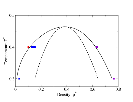
Figure 1: Low density/High density solution phase diagram for the tWF potential used in this work. The solid lines are the liquid-liquid binodal and the broken lines are the spinodal. The points indicate stable (circle) and metastable (squares) systems discussed in the text. For the (weak solution) metastable systems, the corresponding stable (dense liquid) states are also indicated.

The two-parameter models constructed above require only the bulk equation of state and the surface-tension parameter as inputs. Our model system consists of globular proteins in solution, for which the assumption of diffusion-limited dynamics is reasonable. In this Section, we present numerical calculations based on an equation of state derived from the ten Wolde-Frenkel model pair potential for globular proteinsten Wolde and Frenkel (1997b),

$$v\left(r\right)=\left\{\begin{array}[c]{c}\infty,\;\;r\leq\sigma\\ \,\frac{4\,\epsilon}{\alpha^{2}}\left(\,\left(\frac{1}{(\frac{r}{\sigma})^{2}-1}\right)^{6}-\,\alpha\,\left(\frac{1}{(\frac{r}{\sigma})^{2}-1}\right)^{3}\right),\;\;r\geq\sigma\end{array}\right.$$ (37)

using the standard value $\alpha=50$ and cutoff at $r_{c}=2.5\sigma$ and shifted so that $v\left(r_{c}\right)=0$. The parameter $\sigma$ corresponds to the physical size of the globular protein molecule and $\epsilon$ could be determined by fitting to the second-virial coefficient in a weak solution. In the following, numerical results will always be reported in reduced units using $\sigma$ and $\epsilon$ to scale lengths and energies respectively. Reduced quantities will be marked with an asterisk, e.g. reduced temperature is $T^{*}\equiv k_{B}T/\epsilon$ where $k_{B}$ is Boltzmann’s constant. The equation of state was calculated using thermodynamic perturbation theory with a hard-sphere reference state as discussed in Ref. [Lutsko, 2011b]. Figure 1 shows the phase diagram for the low-concentration/high-concentration liquid phases (equivalent to a vapor-liquid phase diagram for a one component system). The surface-tension at coexistence (as required for the free energy model) was calculated using a previously derived approximation, also based only on the pair-potentialLutsko (2011b). Figure 2 shows the free energy surfaces for the system in a sub-critical and a super-critical state. The equilibrium basin is composed of two regions: one with large radius and small deviations of the density from the background (long-wavelength fluctuations), the other having small radius and significant deviations from the background (small, dense, unstable clusters).

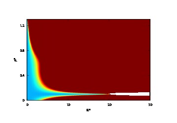
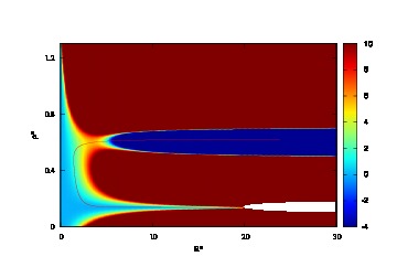
Figure 2: Free energy surfaces for the system in a sub-critical (left panel, $\rho_{\infty}^{*}=0.10$) and super-critical (right panel, $\rho_{\infty}^{*}=0.1375$) state for the model with parameters $\lambda=10$ and $\Delta R_{10}^{*}=20$ and for $T^{*}=0.4$. For display purposes, he free energy values shown are truncated so that what is shown is $\min(10,\max(-4,\beta\Delta\Omega))$. Both panels show similar extended “equilibrium” basins ($0\leq\beta\Delta\Omega\lesssim 1$, light blue) and physically forbidden regions (white) which the model cannot access. The super-critical system has a critical point with energy $\beta\Delta\Omega=5$ and also shows the stable basin at large radii and densities (dark blue): in reality, the free energy drops indefinitely with increasing radius. The right panel also shows the most likely path for nucleation (red line, as calculated in the weak noise limit, see discussion in Section IV.3).

The effect of the parameters $\Delta R_{10}$ and $\lambda$ are illustrated in Fig. 3. When $\lambda=0$, there is a fixed, finite amount of matter available to build a cluster and only a part of the parameter space is accessible. This is equivalent to a finite system and could be used to study nucleation under this constraint. As $\lambda$ increases, allowing for growth of the depletion region with growing cluster size, more of the parameter space becomes accessible until for $\lambda=10$ nearly all of the parameter space is accessible except for a small region near the background region having radius greater than $\Delta R_{10}$. In all cases, $\Delta R_{10}$ limits the size of small amplitude clusters.

Figure 3: The accessible parameter space for a background density $\rho_{\infty}^{*}=0.15$. The parameter $\Delta R_{10}^{*}$ is fixed at $20$ and the effect of different values of $\lambda$ is shown. In each case, the area to the right and between the two branches is inaccessible. For large values of $\lambda$ this reduces to a narrow region around the background density having radius greater than $\Delta R_{10}$.

IV.2 The sub-critical equilibrium state

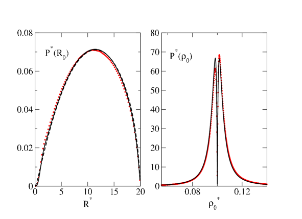
Figure 4: Marginal probability densities for the radius (left panel) and the central density (right panel) of clusters for a sub-critical system. The points were determined using histograms constructed from numerical simulation of the stochastic differential equations. The dashed line is the approximation given in Eq.(36). The state conditions were $T^{*}=0.4$, $\lambda^{*}=20$ and $\rho^{*}_{\infty}=0.10$.

One of our main goals in this Section is to compare our analytic approximations to direct numerical simulation of the stochastic model, Eq. 3. The stochastic simulations were carried out using a Milstein scheme with a variable time-stepGaines and Lyons (1997); Sotiropoulos and Kaznessis (2008); Ilie (2012) as described in Appendix D. Figure 4 shows the marginal probability density for the radius and density as determined by numerical integration of the joint distribution, Eq.(9) evaluated using the explicit forms for the free energy, Eq.(12) and for the determinant of the matrix of kinetic coefficients, Eq.(48)-(58), and by simulation of the stochastic differential equations for a period of $t^{*}=5\times 10^{6}$. Very good numerical agreement is found and further comparisons have shown that the agreement varies systematically with the quality control of the stochastic simulations (see the discussion in Appendix D). The analytic approximation for the marginal probability density for the radius, Eq.(36) is also shown in the Figure and is clearly a very good approximation.

IV.3 The Nucleation Pathway

With more than one order parameter, there are many ways to transition from the meta-stable to the stable state. In fact, there is not even an a priori guarantee that the typical nucleation pathway will pass through (or near) the critical cluster. Nevertheless, it can be shownLutsko (2011a, 2012a) that given the particular structure of the stochastic model used here and working in the weak noise limit, the most likely path (MLP) does indeed pass through the critical cluster and that it can be determined by starting at the critical cluster, perturbing slightly and integrating the deterministic force,

$$\frac{dx^{i}}{dt}=-Dg^{ij}\frac{\partial\beta\Omega}{\partial x^{j}}.$$ (38)

The separatrix is the line between the basin of attraction of the two metastable states. It can be calculated in a similar manner by reversing the sign of the gradient of the free energy in Eq.(38), perturbing slightly in the direction of the stable eigenvector and integrating numerically.

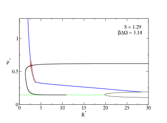
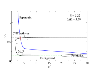
Figure 5: The structure of parameter space for the case of nucleation barrier $\beta\Delta\Omega=3.14$, left panel, and $\beta\Delta\Omega=5.59$, right panel. The initial state is one of constant density indicated by the lower dashed line. The MLP, as calculated from Eq.(38), is shown and, in the right hand panel, its three elements are indicated by arrows: the initial compactification stage that begins at large radius and small density deviation from the background, the densification stage and the final growth stage. The latter is very close to the CNT pathway, indicated by the upper dashed line. The separatrix and forbidden regions are shown as is the critical cluster (the circle at the intersection of the separatrix and the MLP). Finally, the figures also show the crossing points from numerous numerical simulations of the stochastic model (open diamonds). For the smaller cluster, on the left, these are widely distributed along the separatrix whereas for the slightly larger cluster on the right, they are already highly concentrated near the critical cluster.

Figure 5 shows examples of the result of this procedure. It is perhaps surprising that the MLP begins with a cluster having large radius but very small density change from the background: what might be termed a long-wavelength density fluctuation. The MLP then passes through three phases. In the first, the radius decreases while the density increases slowly. In the second phase, there is a rapid densification with little change in radius. The third phase involves growth of the cluster with very slow change in density, which is near that of the dense phase, and is very close to the CNT pathways (as shown in the Figure). This three-stage process is qualitatively identical to what is seen using the full fluctuating hydrodynamic theoryLutsko (2011a, 2012a) and so gives us confidence in the relevance of our model.

We have also performed numerical simulations of the stochastic model (i.e. Eq.(3)). For these, which we term “brute force simulations”, the system began in a random state near the background and was allowed to evolve until the trajectory crossed the separatrix. Figure 5 shows the crossing points obtained from numerous independent simulations. For the smallest cluster, with energy barrier $\Delta\Omega\approx 2k_{B}T$, the crossing points are widely distributed along the separatrix and therefore show the breakdown of the weak noise assumption. However, even for a slightly larger barrier, $\Delta\Omega\approx 5.5$, the crossings are localized very near to the critical cluster, providing evidence that the weak-noise approximation is applicable.

The brute force method is only practical when the energy barriers are relatively small since the mean first passage time increases exponentially with the height of the barrier. We therefore have used Forward Flux Sampling (FFS)Allen et al. (2009) to follow the behavior of systems with larger barriers. The procedure begins with a definition of the metastable basin: we take this to be the region bounded by the $\Delta\Omega=1k_{B}T$ free energy line (with density greater than the background). Next, it is necessary to define a set of intermediate surfaces (lines in the two-dimensional case) between that defining the metastable basin and the separatrix. We take advantage of the similarity in shape between these two lines (compare Figures 2 and 5) to construct nested surfaces via a simple interpolation. Specifically, we pick out $100$ points along each curve an pair them. We let parameter $u=0$ correspond to the boundary of the metastable basin and $u=1$ to the separatrix: a surface for any intermediate value of $u$ is constructed by interpolating along the line joining each pair of points to get an appropriate intermediate point a (Euclidean) distance $u$ between the two end points. These points are used to construct a cubic spline which defines the intermediate surface. In this way, a sequence of nested surfaces corresponding to $u=0,u_{1},...,u_{n}=1$ are constructed.

Once the surfaces are constructed, we then perform a simulation starting from a random point within the metastable basin. After an initial “warmup” period, during which the initial condition is forgotten, we monitor each time the stochastic trajectory exits the metastable basin (i.e. crosses the defining surface in the right direction). This is done until a population of $N_{0}$ such crossings have been recorded. The total time required for this to occur, $t_{0}$ is also recorded. We then perform a new series of simulations in which the initial condition is randomly chosen from this population of exit points. If the trajectory returns to the metastable basin, the simulation is terminated. If it first crosses the next surface, then the simulation is again terminated with the crossing point being recorded. This continues until a prescribed number, $N_{1}$, of crossings has been observed. Then, the process is repeated with the crossings of the first surface as the initial condition and the second surface as the end point, etc., until the separatrix is reached. Further details are discussed, e.g., in Ref. Allen et al. (2009). In this way, one obtains information both about the nucleation pathways and the mean first passage time.

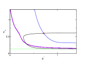
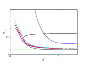
Figure 6: Three steps in the FFS process. The leftmost panel shows the points of exit from the metastable basin; the points map out the border of the metastable state. The central panel shows the points of exit from the second surface. One can see that the population of exit points from the metastable basin has been reduced since not all points generate trajectories that reach the second surface. The rightmost panel shows the next step in the process and how it causes removal of points from both of the previous populations.

Figure 6 shows the way that FFS provides information about the pathway. First, the distribution along the boundary of the metastable region is constructed. Then, this population is used as initial conditions in determining the next set of crossings. Some of the points in the initial population do not spawn trajectories that reach next surface and so they are eliminated. During the next round, some of the points on the second surface do not spawn trajectories crossing the third, so they are dropped. As a result, some of the points on the first surface no longer have daughter points on the second surface so they are also dropped. In this way, each stage results in a refinement that propagates all the way back to the initial population. In the end, all that are left are points that originated a trajectory that reached the separatrix.

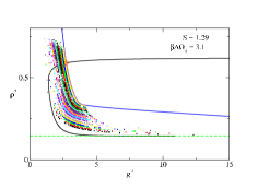
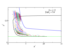
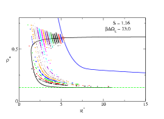
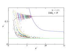
Figure 7: The FFS results for the nucleation pathway for several values of supersaturation spanning the range from very low to moderate nucleation barriers. The energy barriers in each case are given on the figures. At high supersaturation, there is little structure to the nucleation pathway and the crossings of the separatrix are highly dispersed; even at slightly higher supersaturations, the pathway becomes more consistent with the predicted MLP and the crossing of the separatrix is localized to the neighborhood of the critical cluster. Note that the spread of exit points on the separatrix at lower supersaturation is consistent with the results of the brute force calculations as shown in Fig. 5.

Figure 7 shows the FFS information for the nucleation pathway for several different energy barriers. For the most strongly supersaturated systems, there is little structure apparent except for the fact that nearly all successful trajectories begin with low density and finite radii: there are no representative points from the high density, small radius part of the metastable boundary. At lower supersaturation, the structure becomes more apparent and is clearly similar to the MLP calculated in the weak noise limit. The main difference from the MLP is that the densification part of the transition occurs at a somewhat larger radius than the weak noise theory predicts.

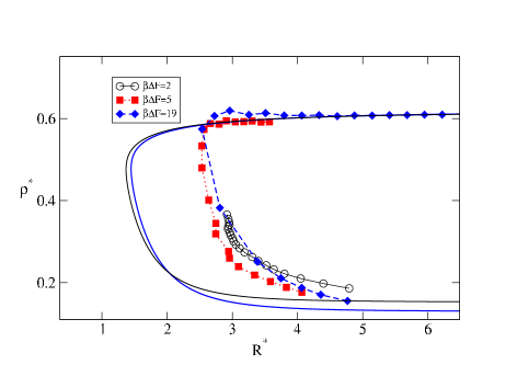
Figure 8: The average pathways as determined from the Forward Flux Sampling simulation data for several values of the nucleation barrier (symbols connected with lines) at $T^{*}=0.40$ . The calculated most likely paths for $\beta\Delta\Omega=2,19$ are shown as well (full lines).

A comparison of the calculated MLP and the average pathways as determined from the FFS simulations using a method discussed in Appendix E is shown in Fig.8. The pathways calculated in the weak-noise limit are in semi-quantitative agreement with the observed pathways although the latter show a systematic shift to larger radii. It is possible that this difference is due to the average pathway being distinct from the most likely pathway but it seems consistent with the raw data as shown in Fig. 7 above. In principle, we could determine the most likely pathway but in attempting to do so we found that our data were too noisy to give convincing results. Figure 9 shows the average paths for a nucleation barrier of $\Delta F=8.2k_{B}T$ for temperatures $T^{*}=0.40$ and $0.30$. At the lower temperature, the MLP shifts towards smaller radii by about $0.5\sigma$ while the shift in the average path is about twice this, thus verifying the expected convergence of the average path to the weak noise result as the temperature is lowered.

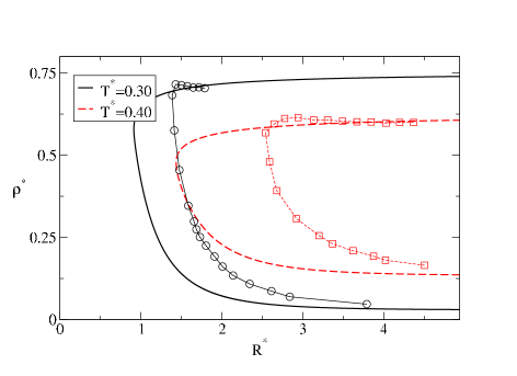
Figure 9: The average pathways as determined from the simulation data for several values of a nucleation barrier of $\Delta\beta F=8.2$ at two different temperatures, $T^{*}=0.30,0.40$. The full lines are the predictions based on the weak-noise approximation and the symbols show the simulation results. Convergence of the simulations to the weak-noise limit as the temperature is lowered is evident.

IV.4 Nucleation Rate

The most important quantity, for practical applications, is the nucleation rate. Here, we compare the time required for nucleation in three approximations. The first is the standard version of CNT for the case of diffusion limited nucleation. In this case, the exact mean first passage time can be calculated numerically using Eq.(19). The second approximation is a modified version of CNT that uses the same model for a mass-conserving cluster as is used in the two-variable theory but with the interior density fixed at the bulk value (as in the usual CNT). This simply means that we replace the free energy and the value of $g_{RR}$ used to reproduce CNT by the equivalent functions evaluated using the mass-conserving cluster profile as inputs to evaluate Eq.(19). The third approximation is the two-variable model for which we only have the approximate expression for the mean first passage time (MFPT), Eq.(10).

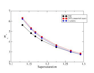
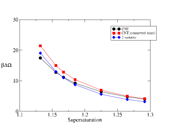
Figure 10: The critical radii (left panel) and energy barriers (right panel) as functions of the supersaturation $S\equiv\rho/\rho_{coex}$. Results are shown are the usual CNT values, Eqs.(17,18) determined by setting $\frac{d}{dR}\beta\Omega=0$ with the density fixed at that of the bulk liquid, the same calculation but using the mass-conserving form of the free energy, Eq.(31), and the result of setting to zero variations of the mass-conserving free energy with respect to both radius and interior density.

Figure 10 shows the radius and excess free energy of the critical cluster as functions of the supersaturation in these three approximations. There is little difference in the radius in the three approximations. The difference in the excess free energy is very small for the highest supersaturations and amounts to about $4k_{B}T$ for the lowest supersaturation. The excess free energy for the two-variable theory is always less than for the mass-conserving CNT as would be expected due to the additional degree of freedom. On the other hand, the usual (non-mass conserving) CNT energy barrier is sometimes higher than for the two-variable theory but not always. This is because with mass-conservation, there is an additional free-energy penalty when forming a cluster due to the cost of the depletion zone.

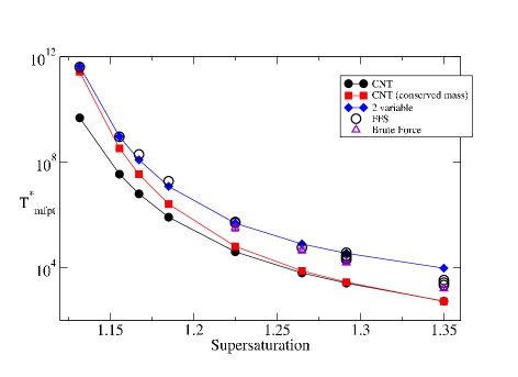
Figure 11: The mean first passage time as a function of the supersaturation $S\equiv\rho/\rho_{coex}$ as determined from the usual CNT, Eq.(19), CNT with the mass-conserving form of the free energy, Eq.(31), the two-variable theory, Eq.(10), and the results of FFS and brute force simulations of the two-variable theory. The brute force values are the result of averaging over an ensemble of approximations 100 trajectories and the standard-deviation is on the order of the symbol-size. At the higher values of supersaturation, multiple FFS determinations were performed varying the random-number generator seed, the number of energy surfaces and the number of crossings of each surface thus giving multiple FFS symbols for some supersaturations: the spread of these results gives some idea of the accuracy of our FFS values.

Figure 11 shows the MFPT as a function of supersaturation as determined from the three approximations as well as from simulation using FFS and, for the systems with the smallest barriers, brute force. First, we note that the FFS and brute force values are mutually consistent thus providing evidence that the FFS implementation is accurate. Second, the times determined from FFS are in remarkable agreement with the approximate times calculated for the two-variable theory except, perhaps, at the highest supersaturation. Given that the analytic theory is only valid in the weak noise limit, this agreement is surprisingly good. Fourth, the mass-conserving CNT seems to converge towards the two-variable theory as supersaturation decreases (i.e. as the critical cluster grows) in line with the general expectation that CNT becomes exact in the limit of large critical clusters. Finally, the MFPT given by the usual CNT is consistently between one and two orders of magnitude below the actual value. This type of discrepancy between CNT and experiment or simulation have often been noted in the literature (some examples are Ref. Ford, 1997; Tanaka et al., 2011, 2014) and are typically attributed to inaccuracies in the calculation of the free energy barrier. However, we show in Fig. 12 the MFPT as a function of the barrier used in the various approximations and it can be seen that this accounts for the difference between CNT with and without mass-conservation, but that in fact the difference from the 2 variable theory cannot be explained on this basis since even with the same energy barrier, the CNT results are consistently between one and two orders of magnitude below the actual MFPT. We conclude that the difference is mostly attributable to the different dynamics and that the inaccuracies in the calculation of the free energy are of secondary importance.

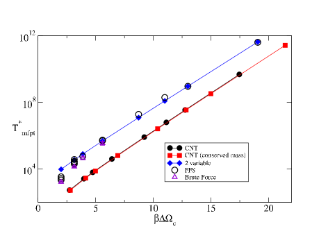
Figure 12: The same as Fig. 11 but showing the mean first passage time as a function of the nucleation barrier. There is a systematic difference between the one- and two-variable theories that cannot be attributed solely to differences in the free energy of the critical cluster.

V Discussion of the results

In this Section, we summarize and attempt to rationalize the various results obtained from our calculations.

V.1 Properties of the critical cluster

• The radius of the critical cluster predicted by CNT is somewhat smaller than that predicted by the mass-conserving theories while there is little difference between the mass-conserving one- and two-variable theories. This larger critical radius is due to the need to offset the increased free-energy penalty arising from the depletion zone.

• The CNT free energy barrier is always smaller than that of the mass-conserving one-variable theory since the latter has an additional free energy penalty due to the lower vapor density in the depletion region. The two variable mass conserving theory has an additional degree of freedom relative to the one-variable mass-conserving theory, so it always has a lower free energy barrier. In the comparison between CNT and the two-variable theory, the two effects (greater free energy penalty and more degrees of freedom) are in play and there is no definitive trend: for smaller clusters, the two-variable theory has lower barrier while for larger clusters, CNT has the smaller barrier. This competition and potential canceling of the two effects can help explain why CNT sometimes appears to be quite accurate.

V.2 Mean first passage times

• Figure 11 shows that the mass-conserving one-variable theory always has larger MFPT (lower nucleation rate) than does CNT and Fig. 12 shows that this is entirely attributable to the difference in free energy barrier. This is therefore an example where “correcting” the calculation of the free energy barrier and using the CNT rate formulas gives the correct nucleation rate.

• The same figures show that the differences between the one-variable and two-variable theories are systematic and cannot be explained solely in terms of poor estimation of free energies. These differences must be attributable to the combination of (a) the calculation of the flux through the critical cluster and (b) the description of the metastable state.

• The calculation of the flux through the critical cluster cannot explain the differences at lower supersaturation (larger nucleation barrier and critical cluster radius). This is because the most likely path, as calculated in the weak noise approximation, pass through the critical cluster in the direction of of the most unstable eigenvector and the figures show that this is nearly parallel to the $R$-axis. In other words, the eigenvalue that occurs in the formula for the MFPT is effectively $g^{RR}\frac{\partial^{2}\Delta F}{\partial R^{2}}$ which is the same quantity as is used in the evaluation of the CNT nucleation rate.

• Consequently, the differences in nucleation rates must be attributable to the calculation of population in the metastable basin. This is clearly very different in the two cases (an exponential distribution in $R$ for CNT versus an algebraic distribution in $R$ for the two-variable theory). Ultimately, this is a reflection of the fact that a theory with long-wavelength, low free-energy fluctuations admits of a much larger accessible phase space than does one with only an isolated minimum on a one-dimensional curve. Put differently, it highlights the failure, within this model, of the common assumption that the probability to observe a cluster of size $N$ is, up to normalization, $e^{-\beta F(N)}$.

• The apparent convergence of the one-variable and two-variable results in Fig. 11 appears to be accidental: the systematic over-estimation of the nucleation barrier in the one-variable theory compensates for the under-estimate of the population of the metastable basin.

V.3 General comments concerning the pathways

• The most likely path calculated in the weak noise limit gives a good semi-quantitative description of the observed average nucleation pathway. Both show the three step process of long-wavelength density fluctuation that contracts followed by densificiation followed by the CNT pathway.

• Both the calculated MLP and the observed average pathways show a minimum cluster size which is consistent with the observations of Trudu et al. Trudu et al. (2006) in simulations of crystallization.

• Since the density fluctuations that become clusters begin with very small density, the usual criterion used in computer simulations for identifying a cluster - namely a group of molecules with local density above some threshhold - is not a good order parameter.

• The numerical results show that the both the calculated most-likely nucleation pathway and the observed average pathway are virtually insensitive to the supersaturation.

• The effect of varying the supersaturation can be viewed as simply moving the position critical cluster along the pathway.

• Only for very small clusters, with barrier less than $5k_{B}T$ do we see any significant crossing away from the neighborhood of the critical cluster.

VI Conclusions

In this paper we have developed a two-variable description of diffusion-limited nucleation based on a formalism developed using fluctuating hydrodynamics. From a purely theoretical perspective, we noted that the most naive generalization of CNT is unphysical. We suggested that this was due to neglect of mass conservation and developed a mass-conserving model that gives qualitatively similar results to those obtained from a direct analysis of the underlying fluctuating hydrodynamics. While in some sense a minimal extension of Classical Nucleation Theory, the model nevertheless illustrates the full complexity of nucleation including strong noise effects and a continuum of possible nucleation pathways. We showed by means of comparison between theory and numerical simulations that both the typical nucleation pathway and the nucleation rate could be accurately determined using results from the weak-noise limit. Finally, this model showed similar deviations from CNT as are commonly reported based on large-scale computer simulation and experiments. Our main practical conclusion was that these differences could not be attributed to errors in the calculation of the free energy barrier but, rather, are a direct result of the more complex dynamics. For this reason, we believe that nucleation can only be properly understood when both thermodynamics and dynamics are incorporated in a self-consistent manner.

The model discussed here therefore provides a sort of “laboratory” within which a variety of post-CNT effects can be studied. We also note that, despite its very different motivations, our model of a cluster - consisting of both a dense core and a low density depletion zone - shares some qualitative similarity to the Extended Modified Liquid Drop ModelReguera and Reiss (2004) of Reiss, Reguera and co-workers. The fact that the core density is allowed to vary and that mass is conserved means that there are also obvious similarities to the Generalized Gibbs approachSchmelzer and Schweitzer (1987); Schmelzer et al. (2006); Schmelzer and Abyzov (2011). The main contribution of the present work is to supplement these ideas with a consistent dynamics that allows for the study of the entire process of nucleation from the initial density fluctuations to the critical cluster and beyond. Nevertheless, in order to tame the divergence of the normalization of the distribution function in subcritical systems while allowing for arbitrary post-critical cluster growth in supersaturated systems, we were forced to introduced a somewhat contrived model. Further studies (not reported here) have shown that the choice of our parameter $\lambda$ has little effect on the properties of nucleation provided the available mass is sufficient to allow for the creation of a critical cluster: this is true even for the extreme case of $\lambda=0$ which corresponds to a fixed volume. This, together with the qualitative agreement with similar work based on the full hydrodynamic model, give us some hope that our results are sufficiently “generic” as to be informative concerning diffusion-limited nucleation in real systems.

Appendix A Density dependence of surface tension

We can gain insight into how the surface tension term should depend on density by starting from a more microscopic perspective. A suitable approximation is the squared-gradient free energy,

$$\Omega[\rho]=\int\left(\omega(\rho(\mathbf{(}r))+g\left(\mathbf{\nabla}\rho(\mathbf{r}\right)^{2}\right)d\mathbf{r}.$$ (39)

This can be derived from exact Density Functional Theory under the assumption that the spatial variation of the density is sufficiently slow[38]. Let us consider the case of a planar interface so that the density depends only on one Cartesian coordinate, say $\rho(z)$ and suppose that the density at $z\rightarrow-\infty$ is equal to the equilibrium density called $\rho_{\infty}$ in the main text. The density at $z\rightarrow\infty$ will be taken to be some small deviation from this value, $\rho_{\infty}+\Delta\rho$. Then, The free energy can be expanded up to second order in the density as

$$\frac{\Omega[\rho]-\Omega(\rho_{\infty})}{A}=\int_{-\infty}^{\infty}\left(\omega^{\prime\prime}(\rho_{\infty})(\Delta\rho(z))^{2}+g\left(\mathbf{\nabla}\Delta\rho(z)\right)^{2}\right)dz$$ (40)

where $A$ is the planar area. The left hand side is just the excess free energy per unit surface (relative to the background). If we assume that the transition from densities close to $\rho_{\infty}+\Delta\rho$ is monotonic and occurs over a spatial region of length $w$, then this will be

$$\frac{\Omega[\rho]-\Omega(\rho_{\infty})}{A}=a_{1}w\omega^{\prime\prime}(\rho_{\infty})(\Delta\rho)^{2}+a_{2}\frac{1}{w}g(\Delta\rho)^{2}$$ (41)

where $a_{1},a_{2}$ are constants dependent on the precise shape of the function $\Delta\rho(z)$. This shows that for fixed width, the surface tension is proportional to the square of the density difference. Rather than fixed width, we might prefer to fix the width by minimizing the free energy. This gives

$$w=\frac{a_{2}g}{a_{1}\omega^{\prime\prime}(\rho_{\infty})}$$ (42)

which is independent of density, so the conclusion remains the same. Similar arguments lead to the same conclusion for liquid-vapor interfaces near coexistence[8, 38]. These facts therefore strongly suggest that the surface tension should vary as the square of the density difference.

Appendix B The kinetic coefficients

For the density parameterization,

$$\rho\left(r\right)=\rho_{0}\Theta\left(R-r\right)+\rho_{1}\Theta\left(r-R\right)\Theta\left(R_{1}-r\right)+\rho_{\infty}\Theta\left(r-R_{1}\right).$$ (43)

the cumulative mass is

$$\Delta m\left(r\right) =\left(\rho_{0}-\rho_{\infty}\right)\left(V\left(r\right)\Theta\left(R-r\right)+V\left(R\right)\frac{R_{1}^{3}-r^{3}}{R_{1}^{3}-R^{3}}\Theta\left(r-R\right)\Theta\left(R_{1}-r\right)\right)$$ (44)

and

$$\frac{\partial\Delta m\left(r\right)}{\partial R} =4\pi\left(\rho_{0}-\rho_{\infty}\right)\frac{R^{2}R_{1}^{2}}{\left(R_{1}^{3}-R^{3}\right)^{2}}\left(R_{1}\left(R_{1}^{3}-r^{3}\right)-\frac{\partial R_{1}}{\partial R}R\left(R^{3}-r^{3}\right)\right)\Theta\left(r-R\right)\Theta\left(R_{1}-r\right)$$ (45)

$$\frac{\partial\Delta m\left(r\right)}{\partial\rho_{0}} =V\left(r\right)\Theta\left(R-r\right)$$

$$+V\left(R\right)\frac{1}{R_{1}^{3}-R^{3}}\left(\left(R_{1}^{3}-r^{3}\right)-\frac{\left(R^{3}-r^{3}\right)}{\left(R_{1}^{3}-R^{3}\right)}3R_{1}^{2}\left(\rho_{0}-\rho_{\infty}\right)\frac{dR_{1}}{d\rho_{0}}\right)\Theta\left(r-R\right)\Theta\left(R_{1}-r\right)$$

A straightforward calculation then gives

$$g_{RR} =\frac{4\pi}{5}\frac{\left(\rho_{0}-\rho_{\infty}\right)^{2}}{\left(\rho_{\infty}-\rho_{0}y^{3}\right)}R^{3}\frac{1}{\left(1+y+y^{2}\right)^{3}}\left(\begin{array}[c]{c}\left(5+6y+3y^{2}+y^{3}\right)+3y^{2}\left(1+3y+y^{2}\right)\frac{dR_{1}}{dR}\\ +y^{3}\left(1+3y+6y^{2}+5y^{3}\right)\left(\frac{dR_{1}}{dR}\right)^{2}\end{array}\right)\allowbreak\allowbreak$$ (48)

$$g_{R\rho_{0}} =\frac{4\pi}{30}\frac{\left(\rho_{0}-\rho_{\infty}\right)}{\rho_{\infty}-\rho_{0}y^{3}}R^{4}\frac{1-y}{\left(1+y+y^{2}\right)^{2}}\left(\begin{array}[c]{c}2\left(5+6y+3y^{2}+y^{3}\right)\\ +3y^{2}\left(1+3y+y^{2}\right)\frac{dR_{1}}{dR}\\ +3y\left(1+3y+y^{2}\right)\left(\frac{3}{R_{1}}\frac{\left(\rho_{0}-\rho_{\infty}\right)}{\left(1-y^{3}\right)}\frac{dR_{1}}{d\rho_{0}}\right)\\ +2y^{2}\left(1+3y+6y^{2}+5y^{3}\right)\frac{dR_{1}}{dR}\left(\frac{3}{R_{1}}\frac{\left(\rho_{0}-\rho_{\infty}\right)}{\left(1-y^{3}\right)}\frac{dR_{1}}{d\rho_{0}}\right)\end{array}\right)\allowbreak$$ (53)

$$g_{\rho_{0}\rho_{0}} =\frac{4\pi}{45}\frac{R^{5}}{\rho_{0}}+\frac{4\pi}{45}\frac{1}{\left(\rho_{\infty}-\rho_{0}y^{3}\right)}R^{5}\frac{\left(1-y\right)^{2}}{1+y+y^{2}}\left(\begin{array}[c]{c}\left(5+6y+3y^{2}+y^{3}\right)\\ +3y\left(1+3y+y^{2}\right)\left(\frac{3}{R_{1}}\frac{\left(\rho_{0}-\rho_{\infty}\right)}{\left(1-y^{3}\right)}\frac{dR_{1}}{d\rho_{0}}\right)\\ +y\left(1+3y+6y^{2}+5y^{3}\right)\left(\frac{3}{R_{1}}\frac{\left(\rho_{0}-\rho_{\infty}\right)}{\left(1-y^{3}\right)}\frac{dR_{1}}{d\rho_{0}}\right)^{2}\end{array}\right)\allowbreak\allowbreak\allowbreak\allowbreak\allowbreak\allowbreak\allowbreak$$ (57)

where $y\equiv R/R_{1}(R,\rho)$. Assuming that $R_{1}(R,0)>0$ and that both $\partial R_{1}/\partial R$ and $(\rho_{0}-\rho_{\infty})\partial R_{1}/\partial\rho_{0}$ are well-behaved as $\rho_{0}\rightarrow\rho_{\infty}$, the leading order density dependence of the kinetic coefficients becomes

$$g_{RR} \sim(\rho_{0}-\rho_{\infty})^{2}$$ (58)

$$g_{R\rho} \sim(\rho_{0}-\rho_{\infty})$$

$$g_{\rho_{0}\rho_{0}} \sim 1$$

so that $\det g\sim(\rho_{0}-\rho_{\infty})^{2}$ just as in the naive model discussed in the main text. This means that the only way to avoid the divergence of the normalization of the probability density is if the range of $R$ is finite, at least for small density fluctuations.

For the model used in the text, $R_{M}^{3}=\Delta R_{10}^{3}+\lambda\left(\frac{\rho_{0}-\rho_{\infty}}{\rho_{\infty}}\right)^{2}R^{3}$, we have that

$$\frac{\partial R_{1}}{\partial R}=3\lambda\left(\frac{\rho_{0}-\rho_{\infty}}{\rho_{\infty}}\right)^{2}R^{3}$$ (59)

$$\frac{\partial R_{1}}{\partial\rho_{0}}=2\lambda\left(\frac{\rho_{0}-\rho_{\infty}}{\rho^{2}_{\infty}}\right)R^{3}$$

Now, the leading order behavior of the coefficients is

$$g_{RR} =\frac{4\pi}{5}\frac{\left(\rho_{0}-\rho_{\infty}\right)^{2}}{\rho_{\infty}}R^{3}\frac{1}{\left(1-y\right)\left(1+y+y^{2}\right)^{4}}\left(5+6y+3y^{2}+y^{3}\right)$$ (60)

$$g_{R\rho_{0}} =\frac{4\pi}{15}\frac{\left(\rho_{0}-\rho_{\infty}\right)}{\rho_{\infty}}R^{4}\frac{1}{\left(1+y+y^{2}\right)^{3}}\left(5+6y+3y^{2}+y^{3}\right)$$

$$g_{\rho_{0}\rho_{0}} =\frac{4\pi}{45}\frac{R^{5}}{\rho_{\infty}}+\frac{4\pi}{45}\frac{1}{\rho_{\infty}}R^{5}\frac{1-y}{\left(1+y+y^{2}\right)^{2}}\left(5+6y+3y^{2}+y^{3}\right)$$

and

$$\det g=\left(\frac{4\pi}{15}\frac{\rho_{0}-\rho_{\infty}}{\rho_{\infty}}R^{4}\right)^{2}\frac{5+6y+3y^{2}+y^{3}}{\left(1-y\right)\left(1+y+y^{2}\right)^{4}}$$ (61)

Appendix C The amplitude of the noise

The relation between the kinetic coefficients and the amplitude of the noise is

$$g^{ij}=q^{ia}q^{jb}\delta_{ab}$$ (62)

Writing

$$q^{ij}=\left(\begin{array}[c]{cc}a&b\\ c&d\end{array}\right)$$ (63)

we need that

$$a^{2}+b^{2} =g^{11}$$ (64)

$$ac+bd =g^{12}$$

$$c^{2}+d^{2} =g^{22}$$

Since there are more parameters than constraints, we are free to fix one parameter. Choosing $c=0$ gives

$$a^{2} =\frac{g^{11}g^{22}-\left(g^{12}\right)^{2}}{g^{22}}$$ (65)

$$b^{2} =\frac{\left(g^{12}\right)^{2}}{g^{22}}$$

$$d^{2} =g^{22}$$

Appendix D Numerical Integration

D.1 Milstein scheme

The Ito SDE is

$$\frac{dx^{i}}{dt}=-Dg^{ij}\frac{\partial\beta\Omega}{\partial x^{j}}+D\varepsilon^{2}A^{i}+\varepsilon\sqrt{2D}q_{a}^{i}\xi^{a}\left(t\right)$$ (66)

Setting $D=1$ by an appropriate choice of time scale, strong first-order convergence can be achieved with the Milstein scheme[47]

$$x^{i}\left(t+\tau\right)=x^{i}\left(t\right)-\left[g^{ij}\frac{\partial\beta\Omega}{\partial x^{j}}+\varepsilon^{2}A^{i}\right]_{\mathbf{x}\left(t\right)}\tau+2q_{a}^{j}\frac{\partial q_{b}^{i}}{\partial x^{j}}I^{ab}\tau+\varepsilon\sqrt{2}q_{a}^{i}\left(\mathbf{x}\left(t\right)\right)I^{a}\sqrt{\tau}$$ (67)

where

$$I^{a}=\frac{1}{\sqrt{\tau}}\int_{t}^{t+\tau}dW_{t^{\prime}}^{a}=\frac{1}{\sqrt{\tau}}\left(W_{t+\tau}-W_{t}\right)=\xi_{t}\in\mathcal{N}\left(0,1\right)$$ (68)

and the Levy area is

$$I^{ab}=\frac{1}{\tau}\int_{t}^{t+\tau}dW_{t^{\prime}}^{a}dW_{t^{\prime}}^{b}$$ (69)

In particular,

$$I^{aa}=\frac{1}{2}\left(\left(I^{a}\right)^{2}-1\right)$$ (70)

while the off-diagonal terms can be calculated from[47]

$$I^{ab}\simeq\frac{1}{2}I^{a}I^{b}+\sqrt{\rho_{p}}\left(\mu^{a}I^{b}-\mu^{b}I^{a}\right)+\frac{1}{2\pi}\sum_{r=1}^{p}\frac{1}{r}\left\{\zeta_{r}^{a}\left(\sqrt{2}I^{b}+\eta^{b}\right)-\zeta_{r}^{b}\left(\sqrt{2}I^{a}+\eta^{a}\right)\right\}$$ (71)

with

$$\mu^{a},\zeta_{r}^{a},\eta^{a}\in\mathcal{N}\left(0,1\right)$$ (72)

and the constant

$$\rho_{p}=\frac{1}{12}-\frac{1}{2\pi^{2}}\sum_{r=1}^{p}\frac{1}{r^{2}}$$ (73)

for some fixed value of $p$ (typically, $p=5$ or $p=10$[40, 41]).

D.2 Variable time step

When we detect that the integration over a timestep $\delta t$ is too inaccurate (see below), the timestep is halved and an extra point is added. The correct way to do this is via the “Brownian Bridge” technique[39] (see also [40, 41]), whereby the difference

$$W_{n+1}^{\alpha}-W_{n}^{\alpha}=\sqrt{\Delta t_{n}}\xi_{n},\;\xi_{2n}\in\mathcal{N}\left(0,1\right)$$ (74)

is replaced by two stochastic steps

$$W_{2n+1}^{\alpha}-W_{2n}^{\alpha} =\frac{1}{2}\left(W_{n+1}^{\alpha}-W_{n}^{\alpha}\right)+\sqrt{\frac{\Delta t_{n+1}}{2}}\xi_{2n+1}=\sqrt{\Delta t_{n}}\left(\frac{1}{2}\xi_{n}+\frac{1}{2}\xi_{2n+1}\right)$$ (75)

$$W_{2n+2}^{\alpha}-W_{2n+1}^{\alpha} =\frac{1}{2}\left(W_{n+1}^{\alpha}-W_{n}^{\alpha}\right)-\sqrt{\frac{\Delta t_{n+1}}{2}}\xi_{2n+1}=\sqrt{\Delta t_{n}}\left(\frac{1}{2}\xi_{n}-\frac{1}{2}\xi_{2n+1}\right)$$

Thus, we replace the Gaussian deviates

$$I_{n}^{\alpha}\rightarrow\left\{\begin{array}[c]{c}\widetilde{I}_{n}^{\alpha}=\frac{1}{2}I_{n}^{\alpha}+\frac{1}{2}I_{n1}^{\alpha}\\ \widetilde{R}_{n+1/2}^{\alpha}=\frac{1}{2}I_{n}^{\alpha}-\frac{1}{2}I_{n1}^{\alpha}\end{array}\right.,\;\;R_{n1}^{\alpha}\in\mathcal{N}\left(0,1\right)$$ (76)

and

$$x_{n+1/2}^{i} =x_{n}^{i}+\left(\frac{\delta t}{2}\right)A^{i}\left(\mathbf{x}_{n}\right)+\sqrt{2\left(\delta t\right)}q_{\alpha}^{i}\left(\mathbf{x}_{n}\right)\widetilde{I}_{n}^{\alpha}+2\left(\frac{\delta t}{2}\right)q_{\alpha}^{j}\left(\mathbf{x}_{n}\right)\frac{\partial q_{\beta}^{i}\left(\mathbf{x}_{n}\right)}{\partial x_{n}^{j}}I^{\alpha\beta}\left(t,t+\frac{\delta t}{2};\widetilde{\mathbf{R}}_{n}\right)$$ (77)

$$x_{n+1}^{i} =x_{n+1/2}^{i}+\left(\frac{\delta t}{2}\right)A^{i}\left(\mathbf{x}_{n+1/2}\right)+\sqrt{2\left(\delta t\right)}q_{\alpha}^{i}\left(\mathbf{x}_{n+1/2}\right)\widetilde{I}_{n+1/2}^{\alpha}$$

$$+2\left(\frac{\delta t}{2}\right)q_{\alpha}^{j}\left(\mathbf{x}_{n+1/2}\right)\frac{\partial q\left(\mathbf{x}_{n+1/2}\right)}{\partial x_{n+1/2}^{j}}I^{\alpha\beta}\left(t+\frac{\delta t}{2},t+\delta t;\widetilde{\mathbf{R}}_{n+1/2}\right)$$

In practice, it is more convenient to replace all of the $\delta t$’s by half their value so we use the equivalent formulation

$$R_{n}^{\alpha}\rightarrow\left\{\begin{array}[c]{c}\widetilde{R}_{n}^{\alpha}=\frac{1}{\sqrt{2}}R_{n}^{\alpha}+\frac{1}{\sqrt{2}}R_{n1}^{\alpha}\\ \widetilde{R}_{n+1/2}^{\alpha}=\frac{1}{\sqrt{2}}R_{n}^{\alpha}-\frac{1}{\sqrt{2}}R_{n1}^{\alpha}\end{array}\right.,\;\;R_{n1}^{\alpha}\in\mathcal{N}\left(0,1\right)$$ (78)

and

$$x_{n+1/2}^{i} =x_{n}^{i}+\left(\frac{\delta t}{2}\right)A^{i}\left(\mathbf{x}_{n}\right)+\sqrt{2\left(\frac{\delta t}{2}\right)}q_{\alpha}^{i}\left(\mathbf{x}_{n}\right)\widetilde{R}_{n}^{\alpha}$$ (79)

$$+2\left(\frac{\delta t}{2}\right)q_{\alpha}^{j}\left(\mathbf{x}_{n}\right)\frac{\partial q_{\beta}^{i}\left(\mathbf{x}_{n}\right)}{\partial x_{n}^{j}}I^{\alpha\beta}\left(t,t+\frac{\delta t}{2};\widetilde{\mathbf{R}}_{n}\right)$$

$$x_{n+1}^{i} =x_{n+1/2}^{i}+\left(\frac{\delta t}{2}\right)A^{i}\left(\mathbf{x}_{n+1/2}\right)+\sqrt{2\left(\frac{\delta t}{2}\right)}q_{\alpha}^{i}\left(\mathbf{x}_{n+1/2}\right)\widetilde{R}_{n+1/2}^{\alpha}$$

$$+2\left(\frac{\delta t}{2}\right)q_{\alpha}^{j}\left(\mathbf{x}_{n+1/2}\right)\frac{\partial q\left(\mathbf{x}_{n+1/2}\right)}{\partial x_{n+1/2}^{j}}I^{\alpha\beta}\left(t+\frac{\delta t}{2},t+\delta t;\widetilde{\mathbf{R}}_{n+1/2}\right)$$

D.3 Quality Control

A variable time step scheme is desirable due to the fact that both the thermodynamic forces and the kinetic coefficients can be anywhere between zero and divergent in magnitude. In order to provide a quick and easy assessment of the accuracy of the integration scheme, we have two criterion for reducing the time step. The first is if the result of advancing one of the parameters causes it to assume an unphysical value (e.g. the radius or density are less than zero). The thermodynamic forces and kinetic coefficients will in general diverge as these limits are reached thus preventing escape from the physical region but if the time step is too large, the integrator may miss such divergences so reducing the time step is obviously needed.

The second criterion, when all values are physical, is that the distance moved in parameter space is less than some prescribed value, $\Delta s$. The stochastic process itself imposes a Riemannian geometry with a precisely defined measure of distance in parameter space, see e.g. Ref. 14. In principle, given a path defined by $R(t),\rho_{0}(t)$ for some beginning and ending times, $t_{0},t_{1}$, the distance moved, $s$, is

$$s=\int_{t_{0}}^{t_{1}}\left(\sqrt{\frac{dx^{i}(t)}{dt}g_{ij}(x(t))\frac{dx^{j}(t)}{dt}}\right)dt$$ (80)

Rather than evaluate this expression exactly, which would be somewhat expensive, we use the approximation

$$s^{(approx)}=\left(x^{i}(t_{1})-x^{i}(t_{0})\right)(\frac{g_{ij}(t_{0})+g_{ij}(t_{1})}{2}\left(x^{j}(t_{1})-x^{j}(t_{0})\right)$$ (81)

and we reduce the time step whenever $s^{(approx)}>\Delta s$. The results in the main text were obtained for $\Delta s^{*}=0.05$.

Appendix E Calculation of average transition paths

The average pathway from the FFS simulations is determined by the average crossing point of each intermediate surface. For each surface, the simulations provide a population of $N$ crossing points each of which is specified by a set of coordinates (density and radius) which we denote as $(R_{\alpha},\rho_{\alpha})$. Clearly, one cannot simply average the coordinates as this would generally not even produce a point on the surface. Instead, let the curve be parameterized as $(R(u),\rho(u)$ with $0\leq u\leq u_{max}$. Then, the i-th crossing point will correspond to some value $u_{\alpha}$ such that $(R_{\alpha},\rho_{\alpha})=(R(u_{\alpha}),\rho(u_{\alpha}))$. We cannot simply average the values of $u$ since the result would then depend on the chosen parameterization of the curve (for which there are an unlimited number of in-equivalent possibilities). So, for each point we calculate the distance along the surface (which is simply a line in our two-dimensional case) using the natural metric provided by the matrix $g_{ij}$. Specifically,

$$d_{\alpha}=\int_{0}^{u_{\alpha}}\sqrt{\frac{dx^{i}(u)}{du}g_{ij}(\mathbf{x}(u))\frac{dx^{j}(u)}{du}}du$$ (82)

where, as previously, $x^{0}\equiv R$ and $x^{1}\equiv\rho$ and repeated indices are summed. The distances along the curve as calculated here are independent of any reparameterization of the curve and, as well, are covariant with respect to a change of the variables characterizing the cluster. It is therefore these quantities that we average to get the average value of $d$ and from this the coordinates of the average point of crossing.