Approximating the generalized terminal backup problem via half-integral multiflow relaxation

Abstract

We consider a network design problem called the generalized terminal backup problem. Whereas earlier work investigated the edge-connectivity constraints only, we consider both edge- and node-connectivity constraints for this problem. A major contribution of this paper is the development of a strongly polynomial-time $4/3$-approximation algorithm for the problem. Specifically, we show that a linear programming relaxation of the problem is half-integral, and that the half-integral optimal solution can be rounded to a $4/3$-approximate solution. We also prove that the linear programming relaxation of the problem with the edge-connectivity constraints is equivalent to minimizing the cost of half-integral multiflows that satisfy flow demands given from terminals. This observation implies a strongly polynomial-time algorithm for computing a minimum cost half-integral multiflow under flow demand constraints.

1 Introduction

1.1 Generalized terminal backup problem

The network design problem is the problem of constructing a low cost network that satisfies given constraints. It includes many fundamental optimization problems, and has been extensively studied. In this paper, we consider a network design problem called the generalized terminal backup problem, recently introduced by Bernáth and Kobayashi [4].

The generalized terminal backup problem is defined as follows. Let $\mathbb{Q}_{+}$ and $\mathbb{Z}_{+}$ denote the sets of non-negative rational numbers and non-negative integers, respectively. Let $G=(V,E)$ be an undirected graph with node set $V$ and edge set $E$, $c\colon E\rightarrow\mathbb{Q}_{+}$ be an edge cost function, and let $u\colon E\rightarrow\mathbb{Z}_{+}$ be an edge capacity function. A subset $T$ of $V$ denotes the terminal node set in which each terminal $t$ is associated with a connectivity requirement $r(t)\in\mathbb{Z}_{+}$. A solution is a multiple edge set on $V$ containing at most $u(e)$ edges parallel to $e\in E$. The objective is to find a solution $F$ that minimizes $\sum_{e\in F}c(e)$ under certain constraints. In Bernáth and Kobayashi [4], the subgraph $(V,F)$ was required to contain $r(t)$ edge-disjoint paths that connect each $t\in T$ to other terminals. In addition to these edge-connectivity constraints, we consider node-connectivity constraints, under which the paths must be inner disjoint (i.e., disjoint in edges and nodes in $V\setminus T$) rather than edge-disjoint. To avoid confusion, we refer to the problem as edge-connectivity terminal backup when the edge-connectivity constraints are required, and as node-connectivity terminal backup when the node-connectivity constraints are imposed. When $r\equiv 1$, the problem is called the terminal backup problem. Since there is no difference between edge-connectivity and node-connectivity when $r\equiv 1$, these names make no confusion.

The generalized terminal backup problem models a natural data management situation. Suppose that each terminal represents a data storage server in a network, and $r(t)$ is the amount of data stored in the server at a terminal $t$. Backup data must be stored in servers different from that storing the original data. To this end, a sub-network that transfers data stored at one terminal to other terminals is required. We assume that edges can transfer a single unit of data per time unit. Hence, transferring data from terminal $t$ to other terminals within one time unit requires $r(t)$ edge-disjoint paths from $t$ to $T\setminus\{t\}$, which is represented by the edge-connectivity constraints. When nodes are also capacitated, $r(t)$ inner-disjoint paths are required; these requirements are met by the node-connectivity constraints.

The generalized terminal backup problem is interesting also from theoretical point of view. Anshelevich and Karagiozova [1] demonstrated that the terminal backup problem is reducible to the simplex matching problem, which is solvable in polynomial time. On the other hand, when $T=V$, the generalized terminal backup problem is equivalent to the capacitated $b$-edge cover problem with degree lower bound $b(v)=r(v)$ for $v\in V$. Since the capacitated $b$-edge cover problem admits a polynomial-time algorithm, the generalized terminal backup problem is solvable in polynomial time also when $T=V$. Therefore, we may naturally ask whether the generalized terminal backup problem is solvable in polynomial time. Bernáth and Kobayashi [4] proposed a polynomial-time algorithm for the uncapacitated case (i.e., $u(e)=+\infty$ for each $e\in E$) in the edge-connectivity terminal backup. Their result partially answers the above question, but their assumptions may be overly stringent in some situations; that is, their algorithm admits unfavorable solutions that select too many copies of a cheap edge. Moreover, their algorithm cannot deal with the node-connectivity constraints. Unfortunately, when the edge-capacities are bounded or node-connectivity constraints are imposed, we do not know whether the generalized terminal backup problem is NP-hard or admits a polynomial-time algorithm. Instead, we propose approximation algorithms as follows.

Theorem 1.

There exist a strongly polynomial-time $4/3$-approximation algorithm for the generalized terminal backup problem.

The present study contributes two major advances to the generalized terminal backup problem.

• Bernáth and Kobayashi [4] discussed the generalized terminal backup problem in the uncapacitated setting with edge-connectivity constraints, noting that the problem in the capacitated setting is open. Here, we discuss the capacitated setting, and introduce the node-connectivity constraints.

• The generalized terminal backup problem can be formulated as the problem of covering skew supermodular biset functions, which is known to admit a 2-approximation algorithm. On the other hand, as stated in Theorem 1, we develop $4/3$-approximation algorithms, that outperform this 2-approximation algorithm.

Let us explain the second advance more specifically. Given an edge set $F$ and a nonempty subset $X$ of $V$, let $\delta_{F}(X)$ denote the set of edges in $F$ with one end node in $X$ and the other in $V\setminus X$. Let $f^{\lambda}\colon 2^{V}\rightarrow\mathbb{Z}_{+}$ be a function such that $f^{\lambda}(X)=r(t)$ if $X\cap T=\{t\}$, and $f^{\lambda}(X)=0$ otherwise. By the edge-connectivity version of Menger’s theorem, $F$ satisfies the edge-connectivity constraints if and only if $|\delta_{F}(X)|\geq f^{\lambda}(X)$ for each $X\subset V$. Bernáth and Kobayashi [4] showed that the function $f^{\lambda}$ is skew supermodular (skew supermodularity is defined in Section 2). For any skew supermodular set function $h$, Jain [11] proposed a seminal $2$-approximation algorithm for computing a minimum-cost edge set $F$ satisfying $|\delta_{F}(X)|\geq h(X)$, $X\subset V$. Although the node-connectivity constraints cannot be captured by set functions as the edge-connectivity constraints, they can be regarded as a request for covering a skew supermodular biset function, to which the 2-approximation algorithm is extended [8] (see Section 2). Therefore, the generalized terminal backup problem admits 2-approximation algorithms, regardless of the imposed connectivity constraints. One of our contributions is to improve these 2-approximations to $4/3$-approximations.

Both of the above 2-approximation algorithms involve iterative rounding of the linear programming (LP) relaxations. Primarily, their performance analyses prove that the value of a variable in each extreme point solution of the LP relaxations is at least $1/2$. Once this property of extreme point solutions is proven, the variables can be repeatedly rounded until a 2-approximate solution is obtained. Our $4/3$-approximation algorithms are based on the same LP relaxations as the iterative rounding algorithms. We show that, in the generalized terminal backup problem, all variables in extreme point solutions of the relaxation take half-integral values. We also prove that the half-integral solution can be rounded into an integer solution with loss of factor at most $4/3$.

It may be helpful for understanding our result to see the well-studied special case of $T=V$ and $u(e)=1$ for each $e\in E$ (i.e., feasible solutions are simple $r$-edge covers). In this case, our LP relaxation minimizes $\sum_{e\in E}c(e)x(e)$ subject to $\sum_{e\in\delta(v)}x(e)\geq r(v)$ for each $v\in V$ and $0\leq x(e)\leq 1$ for each $e\in E$, where $\delta(v)$ is the set of edges incident to the node $v$. It has been already known that an extreme point solution of this LP is half-integral, and the edges in $\{e\in E\colon x(e)=1/2\}$ form odd cycles. The half-integral variables of the edges on an odd cycle can be rounded as follows. Suppose that edges $e_{1},\ldots,e_{k}$ appear in the cycle in this order, where $k$ is the cycle length (i.e., odd integer larger than one). For each $i,j\in\{1,\ldots,k\}$, we define $x^{\prime}_{i}(e_{j})=1$ if $j\geq i$ and $j\equiv i\bmod 2$, or if $j<i$ and $j\equiv i+1\bmod 2$, and $x^{\prime}_{i}(e_{j})=0$ otherwise. See Figure 1. for an illustration of this definition. Note that exactly $(k+1)/2$ variables in $x^{\prime}_{1}(e_{j}),\ldots,x^{\prime}_{k}(e_{j})$ are equal to one, and the other $(k-1)/2$ variables are equal to zero for each $j$. This means that

$$\sum_{i=1}^{k}\sum_{j=1}^{k}c(e_{j})x^{\prime}_{i}(e_{j})=\sum_{j=1}^{k}c(e_{j})\cdot\frac{k+1}{2}=(k+1)\sum_{j=1}^{k}c(e_{j})x(e_{j}).$$

Let $i^{*}$ minimize $\sum_{j=1}^{k}c(e_{j})x^{\prime}_{i^{*}}(e_{j})$ in $i^{*}\in\{1,\ldots,k\}$. Then, since $\sum_{j=1}^{k}c(e_{j})x^{\prime}_{i^{*}}(e_{j})\leq\sum_{i=1}^{k}\sum_{j=1}^{k}c(e_{j})x^{\prime}_{i}(e_{j})/k$, replacing $x(e_{1}),\ldots,x(e_{k})$ by $x^{\prime}_{i^{*}}(e_{1}),\ldots,x^{\prime}_{i^{*}}(e_{k})$ increases their costs by a factor at most $(k+1)/k\leq 4/3$. We also observe that the feasibility of the solution is preserved even after the replacement. By applying this rounding for each odd cycle, the half-integral solution can be transformed into a $4/3$-approximate integer solution.

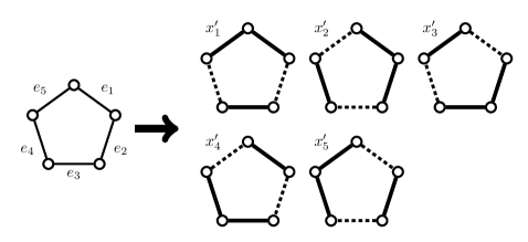
Figure 1: Rounding of half-integral variables corresponding to a cycle of length 5. A dotted line represents $x^{\prime}_{i}(e_{j})=0$, and a solid thick line represents $x^{\prime}_{i}(e_{j})=1$.

Our result is obtained by extending the characterization of the edge structure whose corresponding variables are not integers, but the extension is not immediate. As in the above special case, those edges form cycles in the generalized terminal backup problem if the solution is a minimal feasible solution to the LP relaxation. However, the length of a cycle is not necessarily odd, and it is not clear how the half-integral solution should be rounded; In the above special case, we round up and down variables of edges on a cycle alternatively, but this obviously does not preserve the feasibility in the generalized terminal backup problem. The key ingredient in our result is to characterize the relationship between the cycles and the node sets or bisets corresponding to linearly independent tight constraints in the LP relaxation. We show that a cycle crosses maximal tight node set or bisets an odd number of times, which extends the property that the length of each cycle is odd in the special case. Our rounding algorithm decides how to round a non-integer variable from the direction of the crossing between the corresponding edge and a tight node set or biset.

1.2 Minimum cost multiflow problem

Multiflows are closely related to the generalized terminal backup problem. Among the many multiflow variants, we focus on the type sometimes called free multiflows. For $t,t^{\prime}\in T$, $\mathcal{A}_{t,t^{\prime}}$ denotes the set of paths that terminate at $t$ and $t^{\prime}$. Let $\mathcal{A}_{t}$ denote $\bigcup_{t^{\prime}\in T\setminus\{t\}}\mathcal{A}_{t,t^{\prime}}$, and $\mathcal{A}$ denote $\bigcup_{t\in T}\mathcal{A}_{t}$. $E(A)$ and $V(A)$ denote the sets of edges and nodes in $A\in\mathcal{A}$, respectively. We define a multiflow as a function $\psi\colon\mathcal{A}\rightarrow\mathbb{Q}_{+}$. In the edge-capacitated setting, an edge capacity $u(e)\in\mathbb{Z}_{+}$ is given, and we must satisfy $\sum\{\psi(A)\colon A\in\mathcal{A},e\in E(A)\}\leq u(e)$ for each $e\in E$. In the node-capacitated setting, a node capacity $u(v)\in\mathbb{Z}_{+}$ is given and $\sum\{\psi(A)\colon A\in\mathcal{A},v\in V(A)\}\leq u(v)$ is required for each $v\in V$. The multiflow $\psi$ is called an integral multiflow if $\psi(A)\in\mathbb{Z}_{+}$ for each $A\in\mathcal{A}$, and is called a half-integral multiflow if $2\psi(A)\in\mathbb{Z}_{+}$ for each $A\in\mathcal{A}$. Let $c(A)$ denote $\sum_{e\in E(A)}c(e)$ for $A\in\mathcal{A}$. The cost of $\psi$ is given by $\sum_{A\in\mathcal{A}}\psi(A)c(A)$.

In the edge-connectivity terminal backup, the connectivity requirement from a terminal $t$ equates to requiring that a flow of amount $r(t)$ can be delivered from $t$ to $T\setminus\{t\}$ in the graph $(V,F)$ with unit edge-capacities if $F$ is a feasible solution. This condition appears similar to the constraint that the graph $(V,F)$ with unit edge-capacities admits a multiflow $\psi$ such that $\sum_{A\in\mathcal{A}_{t}}\psi(A)\geq r(t)$. We note that $(V,F)$ with unit edge-capacities admits a multiflow $\psi$ if and only if the number of copies of $e\in E$ in $F$ is at least $\sum_{A\in\mathcal{A}\colon e\in E(A)}\psi(A)$. These observations suggest a correspondence between the edge-connectivity terminal backup and the problem of finding a minimum cost multiflow $\psi$ under the constraint that $\sum_{A\in\mathcal{A}_{t}}\psi(A)\geq r(t)$ for $t\in T$ in the edge-capacitated setting. We refer to such a multiflow computation as the minimum cost multiflow problem (in the edge-capacitated setting). The same correspondence exists between the node-connectivity terminal backup and the node-capacitated setting in the minimum cost multiflow problem.

However, the generalized terminal backup and the minimum cost multiflow problems are not equivalent. Especially, the minimum cost multiflow problem can be formulated in LP, whereas the generalized terminal backup problem is an integer programming problem. Even if multiflows are restricted to integral multiflows, the two problems are not equivalent. To observe this, let $G=(V,E)$ be a star with an odd number of leaves. We assume that $T$ is the set of leaves, and each edge incurs one unit of cost. This star is a feasible solution to the terminal backup problem (i.e., $r(t)=1$ for $t\in T$). In contrast, setting $r\equiv 1$ and $u\equiv 1$ admits no integral multiflow in the edge-capacitated setting, and no feasible (fractional) multiflows in the node-capacitated setting.

Nevertheless, similarities exist between terminal backups and multiflows. As mentioned above, we will show that an LP relaxation of the generalized terminal backup problem always admits a half-integral optimal solution. Similarly, half-integrality results are frequently reported for multiflows. Lovász [14] and Cherkassky [7] investigated $r\equiv 0$ in the edge-capacitated setting, and showed that a half-integral multiflow maximizes $\sum_{A\in\mathcal{A}}\psi(A)$ over all multiflows $\psi$. Using an identical objective function to ours, Karzanov [13, 12] sought to minimize the cost of multiflows. His feasible multiflow solutions are those attaining $\max\sum_{A\in\mathcal{A}}\psi(A)$ in the edge-capacitated setting with $r\equiv 0$, and he showed that the minimum cost is achieved by a half-integral multiflow. Babenko and Karzanov [2] and Hirai [9] extended Karzanov’s result to node-cost minimization in the node-capacitated setting. In this scenario also, the optimal multiflow is half-integral.

In the present paper, we present a useful relationship between the generalized terminal backup problem and the minimum cost multiflow problem in the edge-capacitated setting. We prove that the optimal solution of the LP used to approximate the edge-connectivity terminal backup is a half-integral multiflow, which also optimizes the minimum cost multiflow problem. Thereby, we can compute the minimum cost half-integral multiflow by solving the LP relaxation. This result is summarized in the following theorem.

Theorem 2.

The minimum cost multiflow problem admits a half-integral optimal solution in the edge-capacitated setting, which can be computed in strongly polynomial time.

In contrast, we find no useful relationship between the node-connectivity terminal backup and the node-capacitated setting of the minimum cost multiflow problem. We can only show that the LP relaxation of the node-connectivity terminal backup also has an optimal solution which is a half-integral multiflow in the edge-capacitated setting.

Despite its natural formulation, the minimum cost multiflow problem has not been previously investigated to our knowledge. We emphasize that Theorem 2 cannot be derived from previously known results on multiflows. The minimum cost multiflow problem may be solvable by reducing it to minimum cost maximum multiflow problems that (as mentioned above) admit polynomial-time algorithms. A naive reduction can be implemented as follows. Let $\psi^{*}$ be a minimum cost multiflow that satisfies the flow demands from terminals, and let $\nu(t)=\sum_{A\in\mathcal{A}_{t}}\psi^{*}(A)$ for each $t\in T$. For each $t\in T$, we add a new node $t^{\prime}$ and connect $t$ and $t^{\prime}$ by a new edge of capacity $\nu(t)$. The new terminal set $T^{\prime}$ is defined as $\{t^{\prime}\colon t\in T\}$. Now the multiflow $\psi^{*}$ can be extended to the multiflow of maximum flow value for the terminal set $T^{\prime}$. Applying the algorithm in [13] to this new instance, we can solve the original problem. Moreover, if $\nu(t)$ is an integer for each $t\in T$, this reduction together with the half-integrality result in [12, 13] implies that an optimal multiflow in the minimum cost multiflow problem is half-integral. However, this naive reduction has two limitations. First, $\nu(t)$ is indeterminable without computing $\psi^{*}$. We only know that $\nu(t)$ cannot be smaller than $r(t)$. Second, we cannot ascertain that $\nu(t)$ is always an integer for each $t\in T$. Hence, this naive reduction seems to yield neither a polynomial-time algorithm nor the half-integrality of optimal multiflows claimed in Theorem 2.

Applying a structural result in [4] on the generalized terminal backup problem, it is easily shown that any integral solution to the edge-connectivity terminal backup provides a half-integral multiflow at the same cost. However, since the way to find an optimal solution for the edge-connectivity terminal backup is unknown, Theorem 2 is not derivable from this relationship. In proving the half-integrality of the LP relaxation required for Theorem 1, we immediately imply the quarter-integrality of a minimum cost multiflow (i.e., $4\psi(A)\in\mathbb{Z}_{+}$ for each $A\in\mathcal{A}$). The proof of Theorem 2 requires deeper investigation into the structure of half-integral LP solutions.

1.3 Structure of this paper

Section 2 introduces notations and essential preliminaries on bisets. Section 3 proves that an LP relaxation of the generalized terminal backup problem admits half-integral optimal solutions, and characterizes the edges assigned with half-integral values. Section 4 introduces our $4/3$-approximation algorithm for the generalized terminal backup problem, which proves Theorem 1. Section 5 discusses relationship between the generalized terminal backup and the minimum cost multiflow problems with a proof of Theorem 2. Section 6 concludes the paper.

2 Preliminaries

2.1 Bisets

A biset $\hat{X}$ is defined as an ordered pair $(X,X^{+})$ of node sets $X$ and $X^{+}$ with $X\subseteq X^{+}\subseteq V$. The former and latter elements are respectively called the inner part and outer part of the biset. Throughout the paper, we denote the inner part of a biset $\hat{X}$ by $X$, and the outer part by $X^{+}$. $X^{+}\setminus X$ is called the neighbor of $\hat{X}$, and is denoted by $\Gamma(\hat{X})$. $\mathcal{V}$ is the family of all bisets with nonempty inner parts of $V$. For an edge set $F$ and a biset $\hat{X}$, $\delta_{F}(\hat{X})$ denotes the set of edges in $F$ with one end node in $X$ and the other in $V\setminus X^{+}$. We identify a node $v\in V$ with the biset $(\{v\},\{v\})$. Thereby $\delta_{F}(v)$ denotes the set of edges incident to $v$ in $F$. For simplicity, we write $\delta_{E}(\hat{X})$ as $\delta(\hat{X})$ when the edge set is unambiguously $E$. If an edge $e$ is in $\delta(\hat{X})$, we say that $e$ is incident to $\hat{X}$.

For two bisets $\hat{X}$ and $\hat{Y}$, we define $\hat{X}\cap\hat{Y}$ as $(X\cap Y,X^{+}\cap Y^{+})$, $\hat{X}\cup\hat{Y}$ as $(X\cup Y,X^{+}\cup Y^{+})$, and $\hat{X}\setminus\hat{Y}$ as $(X\setminus Y^{+},X^{+}\setminus Y)$. If $X\subseteq Y$ and $X^{+}\subseteq Y^{+}$, then we write $\hat{X}\subseteq\hat{Y}$. This inclusion relationship defines a partial order on the bisets, from which we define the maximality and minimality among the bisets.

We say that $\hat{X}$ and $\hat{Y}$ are strongly disjoint when $X\cap Y^{+}=\emptyset=X^{+}\cap Y$. If $\hat{X}$ and $\hat{Y}$ are strongly disjoint, $\hat{X}\setminus\hat{Y}=\hat{X}$ and $\hat{Y}\setminus\hat{X}=\hat{Y}$. $\hat{X}$ and $\hat{Y}$ are called noncrossing when strongly disjoint, $\hat{X}\subseteq\hat{Y}$, or when $\hat{Y}\subseteq\hat{X}$. Otherwise, $\hat{X}$ and $\hat{Y}$ are called crossing. A family of bisets is called laminar if each pair of bisets in the family is noncrossing. The laminarity naturally defines a child-parent relationship among bisets (or a forest structure on bisets). Let $\mathcal{L}$ be a laminar family of bisets in $\mathcal{V}$. If $\hat{X},\hat{Y},\hat{Z}\in\mathcal{L}$ satisfy $\hat{X}\subseteq\hat{Y}$ and $\hat{X}\subseteq\hat{Z}$, laminarity implies that $\hat{Y}\subseteq\hat{Z}$ or $\hat{Z}\subseteq\hat{Y}$. Hence, each $\hat{X}\in\mathcal{L}$ admits a unique minimal biset $\hat{Y}\in\mathcal{L}$ with $\hat{X}\subseteq\hat{Y}$ unless $\hat{X}$ is maximal in $\mathcal{L}$. Such a biset $\hat{Y}$ is defined as the parent of $\hat{X}$, and $\hat{X}$ is a child of $\hat{Y}$. This child-parent relationship naturally leads to terminologies such as “ancestor” and “descendant.” For a biset $\hat{Y}$ in a laminar family $\mathcal{L}$ and an edge set $F$, we let $F^{+}_{\mathcal{L}}(\hat{Y})$ and $F^{-}_{\mathcal{L}}(\hat{Y})$ respectively denote $\delta_{F}(\hat{Y})\setminus(\bigcup_{\hat{X}\in\mathcal{X}}\delta_{F}(\hat{X}))$ and $(\bigcup_{\hat{X}\in\mathcal{X}}\delta_{F}(\hat{X}))\setminus\delta_{F}(\hat{Y})$, where $\mathcal{X}$ denotes the set of children of $\hat{Y}$ in $\mathcal{L}$. If $\hat{Y}$ has no child, $F^{+}_{\mathcal{L}}(\hat{Y})=\delta_{F}(\hat{Y})$ and $F^{-}_{\mathcal{L}}(\hat{Y})=\emptyset$.

2.2 Bisets and connectivity of graphs

For $t\in T$, let

$$\mathcal{C}(t)=\{\hat{X}\in\mathcal{V}\colon X\cap T=X^{+}\cap T=\{t\}\}.$$

We denote $\bigcup_{t\in T}\mathcal{C}(t)$ by $\mathcal{C}$. For a vector $x\in\mathbb{Q}_{+}^{E}$ and $E^{\prime}\subseteq E$, let $x(E^{\prime})$ represent $\sum_{e\in E^{\prime}}x(e)$. We define a biset function $f^{\kappa}$ by

$$f^{\kappa}(\hat{X})=\begin{cases}r(t)-|\Gamma(\hat{X})|,&\text{ if }\hat{X}\in\mathcal{C}(t)\text{ for some }t\in T,\\ 0,&\text{ otherwise }\end{cases}$$

for each $\hat{X}\in\mathcal{V}$. According to the node-connectivity version of Menger’s theorem, the graph $(V,F)$ contains $r(t)$ inner-disjoint paths between $t$ and $T\setminus\{t\}$ if and only if $|\delta_{F}(\hat{X})|+|\Gamma(\hat{X})|\geq r(t)$ for each $\hat{X}\in\mathcal{C}(t)$. This condition is equivalent to $|\delta_{F}(\hat{X})|\geq f^{\kappa}(\hat{X})$ for all $\hat{X}\in\mathcal{V}$.

In Section 1, we defined the set function $f^{\lambda}$ representing the edge-connectivity constraints. For treating both node-connectivity and edge-connectivity simultaneously, we sometimes extend $f^{\lambda}$ to a biset function by identifying $X\subseteq V$ with the biset $(X,X)$. Specifically, the biset function $f^{\lambda}$ is defined by

$$f^{\lambda}(\hat{X})=\begin{cases}r(t),&\text{ if }t\in T,\hat{X}\in\mathcal{C}(t),\Gamma(\hat{X})=\emptyset,\\ 0,&\text{ otherwise }\end{cases}$$

for each $\hat{X}\in\mathcal{V}$.

Given a biset function $h$ and an edge-capacity function $u\colon E\rightarrow\mathbb{Z}_{+}$, we define $P(h,u)$ as the set of $x\in\mathbb{Q}_{+}^{E}$ such that

$$x(\delta(\hat{X}))\geq h(\hat{X})\ \ \ \mbox{for $\hat{X}\in\mathcal{V}$}$$ (1)

and

$$x(e)\leq u(e)\text{ for }e\in E.$$

Let $F$ be a multiset of edges in $E$, and $\chi_{F}$ denote the characteristic vector of $F$ (i.e., $\chi_{F}\in\mathbb{Z}_{+}^{E}$ and $F$ contains $\chi_{F}(e)$ copies of $e$ for each $e\in E$). Note that $|\delta_{F}(\hat{X})|=\chi_{F}(\delta(\hat{X}))$ for $\hat{X}\in\mathcal{V}$. Hence, $\chi_{F}\in P(f^{\kappa},u)$ if and only if $F$ is a feasible solution to the node-connectivity terminal backup. Similarly, $\chi_{F}\in P(f^{\lambda},u)$ if and only if $F$ is a feasible solution to the edge-connectivity terminal backup. These statements imply that the LP $\mathsf{LP}(h,u)=\min\left\{\sum_{e\in E}c(e)x(e)\colon x\in P(h,u)\right\}$ relaxes the node-connectivity and the edge-connectivity terminal backups when $h=f^{\kappa}$ and $h=f^{\lambda}$, respectively.

A biset function $h$ is called (positively) skew supermodular when, for any $\hat{X}\in\mathcal{V}$ with $h(\hat{X})>0$ and $\hat{Y}\in\mathcal{V}$ with $h(\hat{Y})>0$, $h$ satisfies

$$h(\hat{X})+h(\hat{Y})\leq h(\hat{X}\cap\hat{Y})+h(\hat{X}\cup\hat{Y})$$ (2)

or

$$h(\hat{X})+h(\hat{Y})\leq h(\hat{X}\setminus\hat{Y})+h(\hat{Y}\setminus\hat{X}).$$ (3)

For any biset function $h$ and a vector $x\colon E\rightarrow\mathbb{Q}_{+}$, we let $h_{x}$ denote the biset function such that $h_{x}(\hat{X})=h(\hat{X})-x(\delta(\hat{X}))$ for each $\hat{X}\in\mathcal{V}$. The skew supermodularity of $f^{\lambda}_{x}$ was reported by Bernáth and Kobayashi [4]. Here, we prove that $f^{\kappa}_{x}$ is also skew supermodular.

Theorem 3.

The biset function $f^{\kappa}_{x}$ is skew supermodular for any $x\colon E\rightarrow\mathbb{Q}_{+}$.

Proof.

Let $\hat{X}$ and $\hat{Y}$ be two bisets. $\hat{X}$ and $\hat{Y}$ are known to always satisfy $|\Gamma(\hat{X})|+|\Gamma(\hat{Y})|\geq|\Gamma(\hat{X}\cap\hat{Y})|+|\Gamma(\hat{X}\cup\hat{Y})|$, $|\Gamma(\hat{X})|+|\Gamma(\hat{Y})|\geq|\Gamma(\hat{X}\setminus\hat{Y})|+|\Gamma(\hat{Y}\setminus\hat{X})|$, $x(\delta(\hat{X}))+x(\delta(\hat{Y}))\geq x(\delta(\hat{X}\cap\hat{Y}))+x(\delta(\hat{X}\cup\hat{Y}))$, and $x(\delta(\hat{X}))+x(\delta(\hat{Y}))\geq x(\delta(\hat{X}\setminus\hat{Y}))+x(\delta(\hat{Y}\setminus\hat{X}))$. These inequalities can be proven by counting contributions of edges on both sides.

Suppose that $f_{x}(\hat{X})>0$ and $f_{x}(\hat{Y})>0$. Then $\hat{X},\hat{Y}\in\mathcal{C}$. If $\hat{X},\hat{Y}\in\mathcal{C}(t)$ for some $t\in T$, then both $\hat{X}\cap\hat{Y}$ and $\hat{X}\cup\hat{Y}$ belong to $\mathcal{C}(t)$. From this statement and the above inequalities, we have $f_{x}(\hat{X})+f_{x}(\hat{Y})\leq f_{x}(\hat{X}\cap\hat{Y})+f_{x}(\hat{X}\cup\hat{Y})$ in this case. If $\hat{X}\in\mathcal{C}(t)$ and $\hat{Y}\in\mathcal{C}(t^{\prime})$ for some $t,t^{\prime}\in T$ with $t\neq t^{\prime}$, then $\hat{X}\setminus\hat{Y}\in\mathcal{C}(t)$ and $\hat{Y}\setminus\hat{X}\in\mathcal{C}(t^{\prime})$. In this case, we have $f_{x}(\hat{X})+f_{x}(\hat{Y})\leq f_{x}(\hat{X}\setminus\hat{Y})+f_{x}(\hat{Y}\setminus\hat{X})$. ∎

3 Structure of extreme point solutions

In this section, we present the properties of the extreme points of $P(f^{\kappa},u)$ and $P(f^{\lambda},u)$. More precisely, we prove that each extreme point of $P(f^{\kappa},u)$ and $P(f^{\lambda},u)$ is half-integral, and that the edges whose corresponding variables are not integers are characteristically structured. Note that both $f^{\kappa}$ and $f^{\lambda}$ are integer-valued skew supermodular functions, and $f^{\kappa}(\hat{X})=f^{\lambda}(\hat{X})=0$ for any $\hat{X}\not\in\mathcal{C}$. In the following, we denote an integer-valued skew supermodular function by $h$, and an extreme point of $P(h,u)$ by $x$.

3.1 Half-integrality

Given an edge set $F$ on $V$ and $\hat{X}\in\mathcal{V}$, let $\eta_{F,\hat{X}}$ denote the characteristic vector of $\delta_{F}(\hat{X})$, i.e., an $|F|$-dimensional vector whose components are set to $1$ if indexed by an edge in $\delta_{F}(\hat{X})$, and $0$ otherwise. The following lemma has been previously proposed [6, 8].

Lemma 1.

Let $h$ be a skew supermodular biset function, and $x$ be an extreme point of $P(h,u)$. Let $E_{0}=\{e\in E\colon x(e)=0\}$, $E_{1}=\{e\in E\colon x(e)=u(e)\}$, and $F=E\setminus(E_{0}\cup E_{1})$. Let $\mathcal{L}$ be an inclusion-wise maximal laminar subfamily of $\{\hat{X}\in\mathcal{V}\colon x(\delta_{F}(\hat{X}))=h(\hat{X})-u(\delta_{E_{1}}(\hat{X}))>0\}$ such that the vectors in $\{\eta_{F,\hat{X}}\colon\hat{X}\in\mathcal{L}\}$ are linearly independent. Then $|F|=|\mathcal{L}|$, and $x$ is a unique vector that satisfies $x(\delta_{F}(\hat{X}))=h(\hat{X})-u(\delta_{E_{1}}(\hat{X}))>0$ for each $\hat{X}\in\mathcal{L}$, $x(e)=0$ for each $e\in E_{0}$, and $x(e)=u(e)$ for each $e\in E_{1}$. Moreover, if some $\hat{Y}\not\in\mathcal{L}$ satisfies $x(\delta_{F}(\hat{Y}))=h(\hat{Y})-u(\delta_{E_{1}}(\hat{Y}))>0$, then $\eta_{F,\hat{Y}}$ is represented as a convex combination of vectors $\eta_{F,\hat{X}}$, $\hat{X}\in\mathcal{L}$.

We note that $\mathcal{L}$ in Lemma 1 can be constructed from the extreme point solution $x$ in a greedy way; initialize $\mathcal{L}$ to an empty set, and repeatedly add a biset $\hat{X}$ such that $x(\delta_{F}(\hat{X}))=h(\hat{X})-u(\delta_{E_{1}}(\hat{X}))>0$, $\eta_{F,\hat{X}}$ is linearly independent from the vectors defined from the bisets in the current $\mathcal{L}$, and adding $\hat{X}$ to $\mathcal{L}$ preserves laminarity of $\mathcal{L}$. Hereafter, we assume that $\mathcal{L}$ is constructed as claimed in Lemma 1. Similarly, $E_{0}$, $E_{1}$, and $F$ are defined from $x$ as in Lemma 1.

Let $\bar{x}\colon E\rightarrow\mathbb{Z}_{+}$, and define a biset function $h_{\bar{x}}(\hat{X})=h(\hat{X})-\bar{x}(\delta(\hat{X}))$ for $\hat{X}\in\mathcal{V}$. Let $\mathbf{1}$ denote the $|E|$-dimensional all-one vector. The following lemma relates only to the extreme points of $P(h_{\bar{x}},\mathbf{1})$. In Corollary 1, we will show that this is sufficient for proving the half-integrality of $P(h,u)$. If $h(\hat{X})>0$ holds only for $\hat{X}\in\mathcal{C}$, we have $\mathcal{L}\subseteq\mathcal{C}$. In this case, no biset in $\mathcal{L}$ has more than one child, and $x$ is characterized as follows.

Lemma 2.

Suppose that $h$ is an integer-valued skew supermodular biset function such that $h(\hat{X})>0$ only for $\hat{X}\in\mathcal{C}$. Let $\bar{x}\colon E\rightarrow\mathbb{Z}_{+}$, and let $x$ be an extreme point of $P(h_{\bar{x}},\mathbf{1})$. Let $F$ denote $\{e\in E\colon 0<x(e)<1\}$. Then the following conditions hold:

1. $|F^{+}_{\mathcal{L}}(\hat{X})|+|F^{-}_{\mathcal{L}}(\hat{X})|=2$ for each $\hat{X}\in\mathcal{L}$;

2. If $e\in F$ is incident to a maximal biset in $\mathcal{L}$, then it is incident to exactly two maximal bisets in $\mathcal{L}$;

3. $x(e)=1/2$ for each $e\in F$.

Proof.

We first prove (i) and (ii) by contradiction. Let us assume that not all of these conditions hold. For each pair of $e\in F$ and its end node $v$, we distribute a token to a biset in $\mathcal{L}$. The biset that obtains the token corresponding to $(e,v)$ is decided as follows:

• If there exist one or more bisets $\hat{X}\in\mathcal{L}$ such that $e\in\delta_{F}(\hat{X})$ and $v\in X$, the token is assigned to the minimal of these bisets.

• Otherwise, the token is assigned to the minimal biset $\hat{Y}$ that includes both end nodes of $e$ in its outer part (if such a biset exists). Notice that such a minimal biset is unique because $\mathcal{L}$ is laminar and $e$ is incident to at least one biset in $\mathcal{L}$.

The total number of tokens is at most $2|F|$. In the following, we prove that tokens may be rearranged so that each biset in $\mathcal{L}$ receives at least two tokens and at least one biset receives three tokens. This rearrangement implies that the number of tokens exceeds $2|\mathcal{L}|$, contradicting our requirement that $|\mathcal{L}|=|F|$.

Recall that $E_{1}=\{e\in E\colon x(e)=1\}$. Let $\bar{x}^{\prime}$ denote $\bar{x}+\chi_{E_{1}}$, and let $\hat{X}$ be a minimal biset in $\mathcal{L}$. The minimality of $\hat{X}$ implies $F^{-}_{\mathcal{L}}(\hat{X})=\emptyset$ and $F^{+}_{\mathcal{L}}(\hat{X})=\delta_{F}(\hat{X})$. Since $x(\delta_{F}(\hat{X}))=h_{\bar{x}^{\prime}}(\hat{X})>0$ and $x(e)<1$ for each $e\in\delta_{F}(\hat{X})$, we have $|F^{+}_{\mathcal{L}}(\hat{X})|=|\delta_{F}(\hat{X})|\geq 2$. Since each edge in $\delta_{F}(\hat{X})$ allocates one token to $\hat{X}$, $\hat{X}$ obtains at least two tokens. If $\hat{X}$ violates (i), then $|F^{+}_{\mathcal{L}}(\hat{X})|=|\delta_{F}(\hat{X})|\geq 3$, and $\hat{X}$ obtains at least three tokens.

Next, let $\hat{X}$ be a biset in $\mathcal{L}$ that admits a child $\hat{Y}\in\mathcal{L}$. Since $\eta_{F,\hat{X}}$ and $\eta_{F,\hat{Y}}$ are linearly independent, $|F_{\mathcal{L}}^{+}(\hat{X})|+|F^{-}_{\mathcal{L}}(\hat{X})|>0$. Therefore, if $h_{\bar{x}^{\prime}}(\hat{X})=h_{\bar{x}^{\prime}}(\hat{Y})$, then $|F_{\mathcal{L}}^{+}(\hat{X})|\geq 1$ and $|F^{-}_{\mathcal{L}}(\hat{X})|\geq 1$. If $h_{\bar{x}^{\prime}}(\hat{X})>h_{\bar{x}^{\prime}}(\hat{Y})$, then $|F_{\mathcal{L}}^{+}(\hat{X})|\geq 2$ because $x(e)<1$, $e\in F_{\mathcal{L}}^{+}(\hat{X})$. Similarly, if $h_{\bar{x}^{\prime}}(\hat{X})<h_{\bar{x}^{\prime}}(\hat{Y})$, then $|F_{\mathcal{L}}^{-}(\hat{X})|\geq 2$. In summary, either case yields $|F_{\mathcal{L}}^{+}(\hat{X})|+|F^{-}_{\mathcal{L}}(\hat{X})|\geq 2$. Since $\hat{X}$ receives a token from each edge in $F_{\mathcal{L}}^{+}(\hat{X})\cup F^{-}_{\mathcal{L}}(\hat{X})$, it obtains at least two tokens and at least three tokens if condition (i) is violated.

Extending the above discussion, each biset in $\mathcal{L}$ obtains at least two tokens, implying that the number of tokens is at least $2|\mathcal{L}|$. If (i) is violated for any biset in $\mathcal{L}$, that biset receives more than two tokens. Now suppose that (ii) is violated. Then there exists an edge $e\in F$ incident to exactly one maximal biset $\hat{X}$ in $\mathcal{L}$. The relation $e\in\delta_{F}(\hat{X})$ indicates that $e$ has an end node $v\in V\setminus X^{+}$, and the token corresponding to $(e,v)$ is assigned to no biset in $\mathcal{L}$. Therefore, if either (i) or (ii) is violated, the number of tokens exceeds the required $2|\mathcal{L}|$.

Let $y\in\mathbb{Q}_{+}^{E}$ be the vector with components $y(e)=1/2$ for each $e\in F$, and $y(e)=x(e)$ for each $e\in E\setminus F$. Let $\hat{X}\in\mathcal{L}$, and denote the child of $\hat{X}$ (if it exists) by $\hat{Y}$. From the above discussion, we obtain the following statements:

• $h_{\bar{x}}(\hat{X})=1$ and $|\delta_{F}(\hat{X})|=2$ if $\hat{X}$ is minimal;

• $|F^{+}_{\mathcal{L}}(\hat{X})|=|F^{-}_{\mathcal{L}}(\hat{X})|=1$ if $\hat{X}$ is not minimal and $h_{\bar{x}}(\hat{X})=h_{\bar{x}}(\hat{Y})$;

• $|F^{+}_{\mathcal{L}}(\hat{X})|=2$, $|F^{-}_{\mathcal{L}}(\hat{X})|=0$ and $h_{\bar{x}}(\hat{X})=h_{\bar{x}}(\hat{Y})+1$ if $\hat{X}$ is not minimal and $h_{\bar{x}}(\hat{X})>h_{\bar{x}}(\hat{Y})$;

• $|F^{+}_{\mathcal{L}}(\hat{X})|=0$, $|F^{-}_{\mathcal{L}}(\hat{X})|=2$, and $h_{\bar{x}}(\hat{X})+1=h_{\bar{x}}(\hat{Y})$ if $\hat{X}$ is not minimal and $h_{\bar{x}}(\hat{X})<h_{\bar{x}}(\hat{Y})$.

Therefore, $y$ satisfies $y(\delta(\hat{X}))=h_{\bar{x}}(\hat{X})$ for each $\hat{X}\in\mathcal{L}$. Since this condition is also uniquely satisfied by vector $x$, we have $x=y$, which proves (iii). ∎

Corollary 1.

Suppose that $h$ is a skew supermodular biset function such that $h(\hat{X})>0$ only if $\hat{X}\in\mathcal{C}$. Let $u\colon E\rightarrow\mathbb{Z}_{+}$. Given $x\in P(h,u)$, we define $\bar{x}\colon E\rightarrow\mathbb{Z}_{+}$ and $x^{\prime}\colon E\rightarrow\mathbb{Q}_{+}$ by $\bar{x}(e)=\lfloor x(e)\rfloor$ and $x^{\prime}(e)=x(e)-\bar{x}(e)$, respectively for each $e\in E$. If $x$ is an extreme point of $P(h,u)$, then $x^{\prime}$ is an extreme point of $P(h_{\bar{x}},\mathbf{1})$. Moreover, $P(h,u)$ is half-integral if $h$ is integer-valued.

Proof.

Note that $0\leq x^{\prime}(e)<1$ for $e\in E$ and $x^{\prime}(\delta(\hat{X}))=x(\delta(\hat{X}))-\bar{x}(\delta(\hat{X}))\geq h(\hat{X})-\bar{x}(\delta(\hat{X}))=h_{\bar{x}}(\hat{X})$ for $\hat{X}\in\mathcal{V}$. Hence, $x^{\prime}\in P(h_{\bar{x}},\mathbf{1})$. In the following, we show that $x^{\prime}$ is an extreme point of $P(h_{\bar{x}},\mathbf{1})$ if $x$ is an extreme point of $P(h,u)$. This proves that $x$ is half-integral because $P(h_{\bar{x}},\mathbf{1})$ is half-integral by Lemma 2.

If $x^{\prime}$ is not an extreme point of $P(h_{\bar{x}},\mathbf{1})$, there exist $y,y^{\prime}\in P(h_{\bar{x}},\mathbf{1})$ and a real number $\alpha$ such that $x^{\prime}=\alpha y+(1-\alpha)y^{\prime}$ and $0<\alpha<1$. Then, $x=x^{\prime}+\bar{x}=\alpha(y+\bar{x})+(1-\alpha)(y^{\prime}+\bar{x})$. Note that both of $y+\bar{x}$ and $y^{\prime}+\bar{x}$ are contained in $P(h,u)$, implying that $x$ is not an extreme point of $P(h,u)$. ∎

3.2 Path decompositions of extreme point solutions

We denote $\{\hat{X}\in\mathcal{L}\colon t\in X\}$ by $\mathcal{L}(t)$ for each $t\in T$. Let $t\in T$ with $\mathcal{L}(t)\neq\emptyset$, and let $\hat{X}_{t}$ be the maximal biset in $\mathcal{L}(t)$. We obtain a graph $G^{s}[\hat{X}_{t}]$ from $G$ by shrinking all the nodes in $V\setminus X^{+}_{t}$ into a single node $s$. Removing $s$ from $G^{s}[\hat{X}_{t}]$, we obtain another graph $G[\hat{X}_{t}]$ (i.e., $G[\hat{X}_{t}]$ is the subgraph of $G$ induced by $X^{+}_{t}$). We suppose that each edge $e$ in $G^{s}[\hat{X}_{t}]$ or in $G[\hat{X}_{t}]$ is capacitated by $x(e)$. If $h=f^{\kappa}$, each node $v$ in $G^{s}[\hat{X}_{t}]$ except $s$ and $t$ has unit capacity. When $h=f^{\lambda}$, each node has unbounded capacity. The capacities of $s$ and $t$ are always unbounded. Since all capacities are half-integral, the maximum flow between $s$ and $t$ in $G^{s}[\hat{X}_{t}]$ can be decomposed into a set of paths $R^{t}_{1},\ldots,R^{t}_{2r(t)}$ each of which accommodates a half unit of flow.

Let $\hat{Y}\in\mathcal{L}(t)$. Each path between $s$ and $t$ passes through an edge in $\delta(\hat{Y})$ or a node in $\Gamma(\hat{Y})$. Since $x(\delta(\hat{Y}))+|\Gamma(\hat{Y})|=r(t)$, the edges in $\delta(\hat{Y})$ and nodes in $\Gamma(\hat{Y})$ are used to full capacity by the maximum flow, and each path $R^{t}_{i}$ includes exactly one edge in $\delta(\hat{Y})$ or one node in $\Gamma(\hat{Y})$.

Suppose that both $R^{t}_{i}$ and $R^{t}_{j}$ include a node $v\not\in\{s,t\}$. Let $e_{i}$ and $e^{\prime}_{i}$ be the edges incident to $v$ on $R^{t}_{i}$, where $e_{i}$ is near to $s$ than $e^{\prime}_{i}$. We define the edges $e_{j}$ and $e^{\prime}_{j}$ incident to $v$ on $R^{t}_{j}$, similarly. We assume that the following fact holds for any such paths $R^{t}_{i}$ and $R^{t}_{j}$.

Assumption 1.

If $x(e_{i})$ is half-integral and $x(e_{j})$ is an integer, and if exactly one of $x(e^{\prime}_{i})$ and $x(e^{\prime}_{j})$ is half-integral, then $x(e^{\prime}_{i})$ is half-integral.

Indeed, if Assumption 1 does not hold, then exchanging the subpaths between $v$ and $t$ makes them satisfy it.

In the following discussion, we consider a maximum flow between a terminal $t^{\prime}$ and $T\setminus\{t^{\prime}\}$ in $G$, where $t^{\prime}$ may equal $t$. In such a flow, each edge $e$ is capacitated by $x(e)$, and each node $v\in V\setminus T$ is assigned the unit capacity or an unbounded capacity if $h=f^{\kappa}$ or $h=f^{\lambda}$, respectively. The capacities of the terminals are assumed as unbounded. The flow quantity for each $t^{\prime}$ is at least $r(t^{\prime})$ if and only if $x$ satisfies (1). Let $\mathcal{S}$ be a path decomposition of the flow between $t^{\prime}$ and $T\setminus\{t^{\prime}\}$, in which each path in $\mathcal{S}$ accommodates a half unit of flow. Let $\mathcal{S}_{t}$ be the set of paths in $\mathcal{S}$ that contain nodes in $X^{+}_{t}$ (recall that $\hat{X}_{t}$ is the maximal biset in $\mathcal{L}(t)$). Without loss of generality, we can state the following fact.

Assumption 2.

Each path in $\mathcal{S}_{t}$ ends at $t$. For a path $S\in\mathcal{S}_{t}$, let $S^{\prime}$ be the subpath of $S$ between $t$ and the nearest node in $V\setminus X^{+}_{t}$. Then, $\{S^{\prime}\colon S\in\mathcal{S}_{t}\}\subseteq\{R_{1}^{t},\ldots,R^{t}_{2r(t)}\}$ holds.

If Assumption 2 is not satisfied by $\mathcal{S}$, we can modify the flow between $t^{\prime}$ and $T\setminus\{t^{\prime}\}$ by replacing the subpaths of those in $\mathcal{S}_{t}$ by appropriate paths in $R^{t}_{1},\ldots,R^{t}_{2r(t)}$, without decreasing the amount of flow.

We say that $x$ is minimal in $P(h,u)$ if $x\in P(h,u)$ and no $y\in P(h,u)$ exists such that $x\neq y$ and $x(e)\geq y(e)$ for any $e\in E$. Let edge $e^{\prime}$ be incident to a node in $X^{+}_{t}$. If $x$ is minimal in $P(h,u)$, then $x(e^{\prime})=|\{i=1,\ldots,2r(t)\colon e^{\prime}\in E(R^{t}_{i})\}|/2$; Otherwise, as $x(e^{\prime})$ is decreased, it would remain in $P(h,u)$.

Lemma 3.

Suppose that $h=f^{\kappa}$ or $h=f^{\lambda}$, and let $x$ be an extreme minimal point in $P(h,u)$. Then $x(\delta(v))$ is an integer for each $v\in V$.

Proof.

Define $\bar{x}$ and $x^{\prime}$ from $x$ as in Corollary 1, and define sets $F$ and $\mathcal{L}$ for $x^{\prime}$ and $P(h_{\bar{x}},\mathbf{1})$ as in Lemma 1. In other words, $F=\{e\in E\colon x^{\prime}(e)=1/2\}$, and $\mathcal{L}$ is a maximal laminar subfamily of $\{\hat{X}\in\mathcal{V}\colon x^{\prime}(\delta(\hat{X}))=h_{\bar{x}}(\hat{X})>0\}$ (because $x^{\prime}(e)<1$ for $e\in E$) such that the vectors in $\{\eta_{F,\hat{X}}\colon\hat{X}\in\mathcal{L}\}$ are linearly independent. It suffices to show that $|\delta_{F}(v)|$ is even for each $v\in V$.

Let $v$ be a node with $\delta_{F}(v)\neq\emptyset$. We first observe that $v$ is included by the outer part of some biset in $\mathcal{L}$. Let $e\in\delta_{F}(v)$. There exists some $\hat{X}^{\prime}\in\mathcal{L}$ with $e\in\delta_{F}(\hat{X}^{\prime})$; otherwise a slight decrease in $x$ retains $x$ in $P(h,u)$. Let $\hat{X}$ be the maximal biset such that $\hat{X}^{\prime}\subseteq\hat{X}\in\mathcal{L}$. If $v\not\in X^{+}$, then (ii) of Lemma 2 implies the existence of another biset $\hat{Y}\in\mathcal{L}$ with $e\in\delta_{F}(\hat{Y})$, where $\hat{Y}$ satisfies $v\in Y^{+}$.

We now prove that $|\delta_{F}(v)|$ is even. First, we consider the case of $h=f^{\kappa}$. The laminarity of $\mathcal{L}$ permits two cases: (i) the existence of maximal bisets $\hat{X}_{1},\ldots,\hat{X}_{l}\in\mathcal{L}$ with $v\in\Gamma(\hat{X}_{1})\cap\cdots\cap\Gamma(\hat{X}_{l})$, and (ii) the existence of exactly one maximal biset $\hat{X}\in\mathcal{L}$ with $v\in X$.

First, we consider the case (i). In the following discussion, we show that an even number of edges in $\delta_{F}(v)$ remains in $G[\hat{X}_{i}]$ for each $i\in\{1,\ldots,l\}$. Each edge $e\in\delta_{F}(v)$ is associated with exactly one biset $\hat{X}_{i}$ that includes the both end nodes of $e$ in its outer part. $e$ remains in $G[\hat{X}_{i}]$, and does not remain in $G[\hat{X}_{i^{\prime}}]$ for any $i^{\prime}\in\{1,\ldots,l\}$ with $i^{\prime}\neq i$. Therefore the claim proves that $|\delta_{F}(v)|$ is even. Denote by $t_{i}$ the terminal with $\hat{{X}}_{i}\in\mathcal{L}(t_{i})$. Note that $v$ is included in exactly two paths in $R^{t_{i}}_{1},\ldots,R^{t_{i}}_{2r(t_{i})}$, say $R^{t_{i}}_{1}$ and $R^{t_{i}}_{2}$. $v$ is adjacent to $s$ in $R^{t_{i}}_{1}$ and $R^{t_{i}}_{2}$. For $j\in\{1,2\}$, let $e_{j}$ be the edge that joins $v$ to the neighbor opposite $s$ in $R^{t_{i}}_{j}$. If $e_{1}=e_{2}$, then $x(e_{1})=1$, and $v$ has no incident edge in $F$ remaining in $G[\hat{X}_{i}]$. If $e_{1}\neq e_{2}$, then $x(e_{1})=x(e_{2})=1/2$. Among the edges in $F$ remaining in $G[\hat{X}_{i}]$, these edges alone are incident to $v$. Hence, the number of edges in $F$ remaining in $G[\hat{X}_{i}]$ is zero or two.

We now discuss case (ii). Let $t$ be the terminal with $\hat{X}\in\mathcal{L}(t)$. By laminarity of $\mathcal{L}$, no biset in $\mathcal{L}\setminus\mathcal{L}(t)$ includes $v$ in its outer part. Hence, it suffices to show that an even number of edges in $\delta_{F}(v)$ remains in $G^{s}[\hat{X}]$. At most two paths in $R^{t}_{1},\ldots,R^{t}_{2r(t)}$ pass through $v$, but if no biset in $\mathcal{L}(t)$ includes $v$ in its neighbor, $v$ may not be used to full capacity. However, each edge in $\delta(v)$ is used to full capacity by the minimality of $x$. If $v\neq t$, then $x(\delta(v))=|\{i\colon v\in V(R^{t}_{i})\}|$, and $x(\delta(v))$ is an integer. If $v=t$, then $x(\delta(v))=r(t)$, and $x(\delta(v))$ is again an integer. In either case, $|\delta_{F}(v)|$ is even, which completes the proof for $h=f^{\kappa}$.

The lemma can be similarly proven for $h=f^{\lambda}$. Case (i) does not occur because $\Gamma(\hat{X})=\emptyset$ for each $\hat{X}\in\mathcal{L}$. ∎

4 $4/3$-approximation algorithm for the generalized terminal backup problem

In this section, we prove Theorem 1 by presenting a $4/3$-approximation algorithm for the generalized terminal backup problem. We first explain how our algorithm works for the case of $r\equiv 1$ for smooth understanding. Then, we present a full proof of Theorem 1.

4.1 Algorithm for case of $r\equiv 1$

Our algorithm rounds a half-integral optimal solution to the LP relaxations into an integer solution. Let us assume that a minimal half-integral optimal solution $x$ and a laminar biset family $\mathcal{L}$ in Lemma 1 are given. In what follows, we explain how to round $x$.

When $r\equiv 1$, the edge- and node-connectivity are equivalent. Since the neighbor of each biset in $\mathcal{L}$ is empty, we identify $\mathcal{L}$ with a family of subsets of $V$.

Let $F$ denote $\{e\in E\colon x(e)=1/2\}$. We call the edges in $F$ half-integral edges. $|\delta_{F}(v)|$ is even for each $v\in V$ because $x(\delta(v))$ is an integer by Lemma 3. Hence $F$ can be decomposed into an edge-disjoint set of cycles. Let $H$ be a cycle in the decomposition.

For each $e\in F$, $\mathcal{L}$ contains a node set to which $e$ is incident. Let $\mathcal{L}^{\prime}$ be the subset of $\mathcal{L}$ that consists of the node sets to which edges in $H$ are incident. Since $r\equiv 1$, exactly two edges in $H$ are incident to each node set in $\mathcal{L}^{\prime}$.

Let $t_{1},\ldots,t_{k}$ be the terminals such that $\mathcal{L}(t_{i})\cap\mathcal{L}^{\prime}\neq\emptyset$ for each $i\in\{1,\ldots,k\}$. We can prove that $k$ is an odd number larger than one. For each $i\in\{1,\ldots,k\}$, let $X_{i}$ denote the maximal node set in $\mathcal{L}(t_{i})\cap\mathcal{L}^{\prime}$, and let $H_{i}$ be the subpath of $H$ comprising of edges incident to node sets in $\mathcal{L}(t_{i})\cap\mathcal{L}^{\prime}$. If an edge is incident to both $X_{i}$ and $X_{j}$, the edge is shared by $H_{i}$ and $H_{j}$.

Let $e_{1}=uv\in F$ be an edge incident to $X_{1}$, where we assume without loss of generality that $u\in X_{1}$ and $v\not\in X_{1}$. Consider traversing $E(H)$, starting from $e_{1}$ in the direction from $v$ to $u$. We say that $t_{i}$ appears when we traverse an edge incident to two node sets $X_{i}\in\mathcal{L}(t_{i})$ and $X_{j}\in\mathcal{L}(t_{j})$ with $i\neq j$ in the direction from the end node in $X_{j}$ to the one in $X_{i}$. Without loss of generality, we assume that the terminals appear in the increasing order of subscripts. Therefore, during the traverse of $H$, we first visit edges in $H_{1}$, then those in $H_{2}$, and so on. Suppose that $X\in\mathcal{L}(t_{i})$ and $e\in\delta_{H}(X)$. We say that $e$ is outward with respect to $t_{i}$ if $e$ is traversed from the end node in $X$ to the other. Otherwise, $e$ is called inward. This implies that, during the traverse of $H_{i}$, we first traverse edges inward with respect to $t_{i}$, and then those outward with respect to $t_{i}$.

We define $k$ assignments of labels to the edges in $H$, where each edge is labeled by either “$+$” or “$-$.” Let us define the $i$-th assignment. If $e\in E(H_{i})$, then $e$ is labeled by “$+$.” If $e\in E(H_{j})$ for some $j>i$, then its label is decided by the following rules.

• If $j-i$ is odd and $e$ is outward with respect to $t_{j}$, $e$ is labeled by “$-$.”

• If $j-i$ is odd and $e$ is inward with respect to $t_{j}$, $e$ is labeled by“$+$.”

• If $j-i$ is even and $e$ is outward with respect to $t_{j}$, $e$ is labeled by “$+$.”

• If $j-i$ is even and $e$ is inward with respect to $t_{j}$, $e$ is labeled by“$-$.”

If $e\in E(H_{j})$ for some $j<i$, we assign the opposite label to the above rules; For example, if $i-j$ is odd and $e$ is outward with respect to $t_{j}$, $e$ is labeled by “$+$.”

Note that this assignment is consistent; if $e$ is included in both $H_{j}$ and $H_{j+1}$, then $e$ is outward with respect to $t_{i}$ and inward with respect to $t_{i+1}$, and hence $e$ is assigned the same label from $j$ and $j+1$; $e_{1}$ is shared by $H_{1}$ and $H_{k}$, and similarly it is assigned the same label because $k$ is odd. Figure 2 shows an example of the cycle $H$, and the first assignment of labels to the edges on $H$.

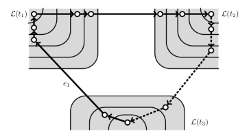
Figure 2: An example of a cycle of half-integral edges and the first assignment of labels to the edges. Edges drawn by solid and dashed lines are assigned “$+$” and “$-$,” respectively. The edges are oriented in the direction of traverse. The areas surrounded by thin solid lines represent the node sets in $\mathcal{L}$.

Our algorithm rounds $x(e)$ into $1$ if $e$ is labeled by “$+$,” and into $0$ otherwise. Since we have $k$ assignments of labels, we have $k$ ways of rounding of variables corresponding to the edges in $H$. Our algorithm chooses the most cost-effective one among them.

Let us observe that this algorithm is $4/3$-approximation. First, we prove that the above rounding increases the cost by a factor of at most $4/3$. Let $x^{\prime}$ be the vector obtained from $x$ by the rounding.

Lemma 4.

$$\sum_{e\in E}c(e)x^{\prime}(e)\leq\frac{4}{3}\sum_{e\in E}c(e)x(e).$$

Proof.

Let $H$ be a cycle of half-integral edges. We show that $\sum_{e\in H}c(e)x^{\prime}(e)\leq\frac{4}{3}\sum_{e\in H}c(e)x(e)$. Applying this claim to all cycles in the decomposition of $F$, we can prove the lemma. We use the notations used in the definition of the rounding.

Let $x_{i}$ denote the vector obtained by rounding $x(e)$, $e\in E(H)$ according to the $i$-th assignment of labels. We note that

$$\sum_{e\in H}c(e)x^{\prime}(e)=\min_{1\leq i\leq k}\sum_{e\in H}c(e)x_{i}(e)\leq\frac{1}{k}\sum_{i=1}^{k}\sum_{e\in H}c(e)x_{i}(e).$$

Recall that $k$ is an odd number larger than one. In the $k$ assignments, $e\in H$ is labeled “$+$” by the $(k+1)/2$ assignments. Thus,

$$\sum_{i=1}^{k}\sum_{e\in H}c(e)x_{i}(e)=\frac{k+1}{2}\sum_{e\in H}c(e).$$

Note that $\sum_{e\in H}c(e)x(e)=\sum_{e\in H}c(e)/2$. Therefore,

$$\frac{\sum_{e\in H}c(e)x^{\prime}(e)}{\sum_{e\in H}c(e)x(e)}\leq\frac{k+1}{k}\leq\frac{4}{3},$$

where the last inequality follows from $k\geq 3$. ∎

Next, let us prove the feasibility of $x^{\prime}$. For a path $P$ and nodes $u,v$ on $P$, we denote the subpath of $P$ between $u$ and $v$ by $P[u,v]$.

Lemma 5.

$x^{\prime}$ is a feasible solution to the terminal backup problem.

Proof.

Obviously $x^{\prime}$ is an integer vector. Hence, to prove the feasibility of $x^{\prime}$, the graph with edge-capacities $x^{\prime}$ admits a unit of flow from each terminal $t$ to the other terminals. Since $x(\delta(X))\geq 1$ for each $X\in\mathcal{C}(t)$, the graph capacitated by $x$ admits such a flow. Hence we show that a flow for $x^{\prime}$ can be obtained by modifying the flow for $x$. In the following, we assume that $x^{\prime}$ is obtained by rounding variables corresponding to the half-integral edges in a cycle $H$. If required, the modification is repeated for each cycle of half-integral edges.

Recall the definition of $R^{t}_{1},\ldots,R^{t}_{2r(t)}$ in Section 3.2. Since we are considering the case of $r\equiv 1$, we have two paths $R^{t}_{1}$ and $R^{t}_{2}$ for each terminal $t$ with $\mathcal{L}(t)\neq\emptyset$. We assume these paths satisfy Assumption 1. Fix a terminal $t$, and suppose that the flow from $t$ to the other terminals with edge-capacities $x$ delivers a half unit of flow along a path $P$, and another half unit along a path $Q$. We assume that $\mathcal{S}=\{P,Q\}$ satisfies Assumption 2.

If both $P$ and $Q$ contains no half-integral edge (with respect to $x$) labeled by “$-$,” the flow satisfies the capacity constraints defined from $x^{\prime}$. Thus, let us consider the case where $P$ includes a half-integral edge labeled by “$-$.” Let $e$ be the one nearest to $t$ among such edges, and let $v$ be the end node of $e$ near to $t$.

We first show that there exists $X^{*}\in\mathcal{L}(t)$ such that $e\in\delta(X^{*})$ and $v\in X^{*}$. For arriving at a contradiction, suppose that such $X^{*}$ does not exist. $e$ is incident to at least one node set in $\mathcal{L}$. In particular, Lemma 2(ii) implies that there exists a terminal $t^{\prime}\in T$ and node set $X^{\prime}\in\mathcal{L}(t^{\prime})$ such that $e\in\delta(X^{\prime})$ and $v\in X^{\prime}$. However, this means that $t^{\prime}\neq t$ and $P[t,v]$ enters $X^{\prime}$ when traversed from $t$ to $v$. Assumption 2 indicates that the subpath of $P$ between $v$ and the end opposite to $t$ is included by $R^{t^{\prime}}_{1}$ or $R^{t^{\prime}}_{2}$. Hence, the end of $P$ opposite to $t$ is $t^{\prime}$, and $P$ does not include $e$, which is a contradiction. Therefore, there exists $X^{*}\in\mathcal{L}(t)$ such that $e\in\delta(X^{*})$ and $v\in X^{*}$.

This fact indicates that $Q$ contains no “$-$”-labeled half-integral edge because of the following reason. Let $P^{\prime}$ be the subpath of $P$ that is included by a maximal node set in $\mathcal{L}(t)$. Since $\mathcal{L}(t)\neq\emptyset$, there exists $R^{t}_{1}$ and $R^{t}_{2}$. By Assumption 2, $P^{\prime}$ is equal to $R^{t}_{1}$ or $R^{t}_{2}$. Without loss of generality, let $P^{\prime}$ be equal to $R^{t}_{1}$. Then, Assumption 1 indicates that all “$-$”-labeled half-integral edges incident to node sets in $\mathcal{L}(t)$ is included in $R^{t}_{1}$. Since $P$ and $Q$ share no half-integral edges, $Q$ does not include these edges in $R^{t}_{1}$. Hence, if $Q$ contains a “$-$”-labeled half-integral edge, its both end node is included by some node sets in $\mathcal{L}\setminus\mathcal{L}(t)$. However, we can derive a contradiction similarly for the above claim with $P$.

Since $x(\delta(X^{*}))=1$, the other edge $e^{\prime}$ incident to $v$ on $H$ is also incident to $X^{*}$. By the label-assignment rules, $e^{\prime}$ is labeled by “$+$.” Let $H^{\prime}$ denote the subpath of $H$ consisting of “$+$”-labeled edges and terminating at $v$. Let $u$ be the other end node of $H^{\prime}$, and let $g$ be the edge incident to $u$ on $H^{\prime}$. By Lemma 2, there exists $Y\in\mathcal{L}$ with $g\in\delta(Y)$ and $u\in Y$. $Y$ belongs to $\mathcal{L}(t^{\prime})$ for some $t^{\prime}\neq t$. $g$ is included in a path $R_{1}^{t^{\prime}}$ or $R_{2}^{t^{\prime}}$. Without loss of generality, we suppose that $R_{1}^{t^{\prime}}$ includes $g$. We replace $P$ by the concatenate of $P[t,v]$, $H^{\prime}$, and $R_{1}^{t^{\prime}}[u,t^{\prime}]$. See Figure 3 for illustration of this modification.

Figure 3: The definitions in the proof of Lemma 5

Let us observe that this modification preserves the capacity constraints. $P[t,v]$ was a part of $P$ before the modification. The capacity of each edge on $H^{\prime}$ is increased by $1/2$ when $x^{\prime}$ replaces $x$. The capacity of each edge in $R_{1}^{t^{\prime}}[u,t^{\prime}]$ is integer. Hence no capacity constraint is violated. ∎

4.2 Algorithm for the general case

In this subsection, we present a strongly polynomial-time algorithm for the generalized terminal backup problem. In the following discussion, $h$ denotes a skew supermodular function such that $h(\hat{X})>0$ only when $\hat{X}\in\mathcal{C}$.

Solving the LP relaxation

We wish to ensure that any optimal solution $x$ to $\mathsf{LP}(h,u)$ is minimal in $\mathsf{LP}(h,u)$. Clearly, this condition holds when $c(e)>0$ for each $e\in E$. If $c(e)=0$ for some $e\in E$, the condition is ensured by perturbing $c$. Since we can restrict our attention to half-integral solutions, it is sufficient to reset $c(e)$ to a positive number smaller than $2/(\theta|E|)$ for each $e$ with $c(e)=0$, where $\theta$ is the maximum denominator of the edge costs.

The number of constraints of $\mathsf{LP}(h,u)$ is exponential; hence, it is unclear how to solve $\mathsf{LP}(h,u)$ in polynomial time. If $h=f^{\kappa}$ or $h=f^{\lambda}$, the separation is reducible to a maximum flow computation, and $\mathsf{LP}(h,u)$ can be solved by the ellipsoid method. Alternatively, the constraints can be written in a compact form by introducing flow variables for each terminal, as implemented in Jain [11]. Hence, if $h=f^{\kappa}$ or $h=f^{\lambda}$, there are two ways of solving $\mathsf{LP}(h,u)$ in polynomial time. However, Theorem 1 claims a strongly polynomial-time algorithm. All coefficients in the constraints of $\mathsf{LP}(h,u)$ are one. Accordingly, Tardos’ algorithm [17] computes an optimal solution to $\mathsf{LP}(h,u)$ in strongly polynomial time, but does not guarantee an extreme point solution.

Our algorithm first finds an optimal solution to $\mathsf{LP}(h,u)$ by Tardos’ algorithm. The obtained solution is denoted by $x^{*}$. Defining $\bar{x}^{*}\colon E\rightarrow\mathbb{Z}_{+}$ by $\bar{x}^{*}(e)=\lfloor x^{*}(e)\rfloor$ for $e\in E$, we then compute an extreme point optimal solution $x$ to $\mathsf{LP}(h_{\bar{x}^{*}},\mathbf{1})$. $\bar{x}^{*}+x$ is not necessarily an extreme point of $P(h,u)$, but is a half-integral optimal solution to $\mathsf{LP}(h,u)$. The following lemma shows that $x$ can be computed by iterating Tardos’ algorithm.

Lemma 6.

An extreme point optimal solution to $\mathsf{LP}(h_{\bar{x}^{*}},\mathbf{1})$ can be computed in strongly polynomial time.

Proof.

As noted above, an optimal solution to $\mathsf{LP}(h_{\bar{x}^{*}},\mathbf{1})$ can be computed in strongly polynomial time. Moreover, whether fixing a variable $x(e)$ to a specific value $\tau$ increases the optimal value is also testable in strongly polynomial time by solving $\mathsf{LP}(h_{\bar{x}^{*}},\mathbf{1})$ with an additional constraint $x(e)=\tau$. We sequentially test fixing the variables $x(e)$ to $0$ or $1$, and if the fix does not increase the optimal value, the variable is set to the fixed value. If $x(e)$ is not fixed to $0$ or $1$, it is set to $1/2$.

Optimality of the above-constructed solution $x$ follows from the existence of a half-integral optimal solution (see Lemma 2). We must now prove that the obtained solution $x$ is an extreme point. If not, $x$ can be represented by $\sum_{i=1}^{l}\alpha_{i}y_{i}$, where $l\geq 2$, $y_{1},\ldots y_{l}$ are extreme points of $P(h_{\bar{x}^{*}},\mathbf{1})$, and $\alpha_{1},\ldots,\alpha_{l}$ are positive real numbers with $\sum_{i=1}^{l}\alpha_{i}=1$. Let $i\in\{1,\ldots,l\}$. The optimality of $x$ indicates that $y_{i}$ is an optimal solution to $\mathsf{LP}(h_{\bar{x}^{*}},\mathbf{1})$. Moreover, $y_{i}(e)=x(e)$ holds if $x(e)\in\{0,1\}$. Therefore, there exists some $e\in E$ such that $x(e)=1/2$ and $y_{i}(e)\in\{0,1\}$, which contradicts the way of constructing $x$. ∎

Let $F=\{e\in E\colon x(e)=1/2\}$. Our algorithm also requires $\mathcal{L}$ defined from $x$ (i.e., $\mathcal{L}$ is a maximal laminar subfamily of $\{\hat{X}\in\mathcal{C}\colon x(\delta_{F}(X))=h_{\bar{x}^{*}}(\hat{X})>0\}$ such that the vectors $\eta_{F,\hat{X}}$, $\hat{X}\in\mathcal{L}$ are linearly independent). As stated in the paragraph following Lemma 1, $\mathcal{L}$ can be constructed by repeatedly adding a biset $\hat{Y}$ in $\{\hat{X}\in\mathcal{C}\colon x(\delta_{F}(X))=h_{\bar{x}^{*}}(\hat{X})>0\}$ such that adding $\hat{Y}$ to $\mathcal{L}$ preserves the laminarity of $\mathcal{L}$ and the linear independence of the vectors $\eta_{F,\hat{X}}$, $\hat{X}\in\mathcal{L}$. If $\mathcal{L}$ is not maximal, such a biset $\hat{Y}$ can be found as follows. By Lemma 2, one of such $\hat{Y}$ satisfies either of the following conditions:

• $\hat{Y}$ is minimal in $\{\hat{Y}\}\cup\mathcal{L}$, and $|\delta_{F}(\hat{Y})|=2$;

• There exits $\hat{X}\in\mathcal{L}$ such that $\hat{X}\subseteq\hat{Y}$ and $|\delta_{F}(\hat{X})\setminus\delta_{F}(\hat{Y})|+|\delta_{F}(\hat{Y})\setminus\delta_{F}(\hat{X})|=2$.

The number of bisets satisfying one of these conditions is strongly polynomial. We can decide in strongly polynomial time whether adding a biset to the current $\mathcal{L}$ preserves the conditions of $\mathcal{L}$. Therefore, $\mathcal{L}$ can computed in strongly polynomial time.

Rounding half-integral solutions to $4/3$-approximate solutions

Our algorithm rounds $x$, the extreme point optimal solution to $\mathsf{LP}(h_{\bar{x}^{*}},\mathbf{1})$, to an integer vector $x^{\prime}\in P(h_{\bar{x}^{*}},\mathbf{1})$ subject to $\sum_{e\in E}c(e)x^{\prime}(e)\leq 4/3\cdot\sum_{e\in E}c(e)x(e)$. It then outputs $\bar{x}^{*}+x^{\prime}$.

The rounding procedure is almost same as the algorithm for $r\equiv 1$. Let $F=\{e\in E\colon x(e)=1/2\}$. By Lemma 3, $|\delta_{F}(v)|$ is even for each $v\in V$ because $\bar{x}^{*}+x$ is minimal in $P(h,u)$. We can see that $|\delta_{F}(v)|$ is an even number at most four.

Lemma 7.

$|\delta_{F}(v)|\leq 4$ for each $v\in V$. If $|\delta_{F}(v)|=4$, there exist $\hat{X},\hat{W}\in\mathcal{L}$ such that $\hat{W}\subseteq\hat{X}$, $v\in X\setminus W^{+}$, and $|\delta_{F}(v)\cap\delta_{F}(\hat{X})|=2=|\delta_{F}(v)\cap\delta_{F}(\hat{W})|$.

Proof.

Let $\delta_{F}(v)\neq\emptyset$. Then, Lemma 2 (ii) implies that $v$ is included in the inner-part of some biset in $\mathcal{L}$. Let $\hat{X}$ be the minimal biset in $\mathcal{L}$ such that $v\in X$. If $\hat{X}$ is minimal in $\mathcal{L}$, then $\delta_{F}(v)\subseteq\delta_{F}(\hat{X})$, and $|\delta_{F}(v)|\leq 2$ follows from $|\delta_{F}(\hat{X})|=2$. In the rest of the proof, suppose that $\hat{X}$ has the child $\hat{Y}\in\mathcal{L}$. Then $v\not\in Y$. Suppose that $v\in Y^{+}$, and let $\hat{Z}$ be the minimal biset in $\mathcal{L}$ such that $\hat{Z}\subseteq\hat{Y}$ and $v\in Z^{+}$, where $\hat{Z}$ is possibly equal to $\hat{Y}$. Let $\hat{W}$ be the child of $\hat{Z}$. Each edge $e\in\delta_{F}(v)$ is incident to $\hat{X}$ or $\hat{W}$. Notice that $e$ is not incident to $\hat{Y}$ or $\hat{Z}$. Hence, $e\in F^{+}_{\mathcal{L}}(\hat{X})$ if $e$ is incident to $\hat{X}$, and $e\in F^{-}_{\mathcal{L}}(\hat{Z})$ if $e$ is incident to $\hat{W}$. Thus $|\delta_{F}(v)|\leq|F^{+}_{\mathcal{L}}(\hat{X})|+|F^{-}_{\mathcal{L}}(\hat{Z})|\leq 4$. If $\hat{W}$ does not exist, $|\delta_{F}(v)|\leq|F^{+}_{\mathcal{L}}(\hat{X})|\leq 2$. If $v\not\in Y^{+}$, we can similarly show that $\delta_{F}(v)\subseteq F^{+}_{\mathcal{L}}(\hat{X})\cup F^{-}_{\mathcal{L}}(\hat{X})$, and hence $|\delta_{F}(v)|\leq 2$ follows from $|F^{+}_{\mathcal{L}}(\hat{X})|+|F^{-}_{\mathcal{L}}(\hat{X})|\leq 2$. ∎

We decompose $F$ into a set of cycles. We assume without loss of generality that the decomposition satisfies the following assumption.

Assumption 3.

Let $v$ be a node such that $|\delta_{F}(v)|=4$. Let $\hat{X},\hat{W}\in\mathcal{L}$ be the bisets such that $\hat{W}\subseteq\hat{X}$, $v\in X\setminus W^{+}$, and $|\delta_{F}(v)\cap\delta_{F}(\hat{X})|=2=|\delta_{F}(v)\cap\delta_{F}(\hat{W})|$. Then the two edges in $\delta_{F}(v)\cap\delta_{F}(\hat{X})$ (resp., $\delta_{F}(v)\cap\delta_{F}(\hat{W})$) are included in the same cycle in the decomposition.

Suppose that $H$ includes an edge incident to a biset in $\mathcal{L}(t_{1})$ and another in $\mathcal{L}(t_{k})$ for some terminals $t_{1},t_{k}$ with $t_{1}\neq t_{k}$. Let $e_{1}$ be one of such edges. We traverse $H$, starting from $e_{1}$. Suppose that $e_{1}$ is traversed from a biset in $\mathcal{L}(t_{k})$ to one in $\mathcal{L}(t_{1})$. Let $(t_{1},\ldots,t_{k})$ be the sequence of terminals that appear when we traverse $H$ from $e_{1}$, where $t_{i}$ denotes the terminal that appears immediately after $t_{i-1}$. A different fact from the case of $r\equiv 1$ is that a terminal can appear more than once during the traverse. Thus $t_{i}$ and $t_{j}$ may stand for the same terminal unless $j\in\{i-1,i+1\}$ or $\{i,j\}=\{1,k\}$.

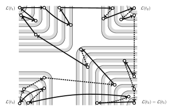
Figure 4: An example of a cycle of half-integral edges and labels assigned to the edges. Edges drawn by solid and dashed lines are assigned “$+$” and “$-$,” respectively. The edges are oriented in the direction of traverse. The areas surrounded by thin solid lines represent the outer parts of bisets in $\mathcal{L}$, and gray areas indicate their neighbors. In this figure, neighbors of bisets in $\mathcal{L}$ are disjoint for visibility, but neighbors can overlap in general.

Let $H_{i}$ be the subpath of $H$ that consists of edges between the appearance of $t_{i}$ and $t_{i+1}$, where $H_{i}$ and $H_{i+1}$ share an edge that is incident to both a biset in $\mathcal{L}(t_{i})$ and one in $\mathcal{L}(t_{i+1})$, and $H_{1}$ and $H_{k}$ share $e_{1}$. We also define “inward” and “outward” edges in $H_{i}$ with respect to $t_{i}$ as in the case of $r\equiv 1$. Another different fact in the general case from the case of $r\equiv 1$ is that the direction of edges on $H_{i}$ with respect to $t_{i}$ changes more than once because $H$ may contain more than two edges incident to a biset in $\mathcal{L}$.

If all edges on $H$ are incident to only bisets in $\mathcal{L}(t)$ for some terminal $t$, we let $k=1$, and $H_{1}=H$ for convention. In the following lemma, we see that $k$ is an odd number larger than one.

Lemma 8.

A cycle such that $k$ is one or an even number does not exist.

Proof.

Suppose that $k$ is one or an even number for a cycle $H$. Let us assign labels to each edge in $H$ as follows. Let $e\in H_{i}$. If $i$ is odd and $e$ is inward to $t_{i}$, or if $i$ is even and $e$ is outward to $t_{i}$, then $e$ is labeled “$-$.” Otherwise, $e$ is labeled “$+$.” We note that, for each $\hat{X}\in\mathcal{L}$, exactly half of the edges in $\delta_{H}(\hat{X})$ are labeled by “$+$.”

Let $\epsilon$ be a constant. For each edge $e$ in $H$, update the corresponding variable $x(e)$ to $x(e)+\epsilon$ if $e$ is labeled by “$+$”, and update to $x(e)-\epsilon$ otherwise. Let $x_{\epsilon}$ denote the obtained vector. The number of labels assigned indicates that $x_{\epsilon}(\delta_{F}(\hat{X}))=x_{-\epsilon}(\delta_{F}(\hat{X}))=h_{\bar{x}^{*}}(\hat{X})$ for each $\hat{X}\in\mathcal{L}$. If $x(\delta_{F}(\hat{Y}))=h_{\bar{x}^{*}}(\hat{Y})$ holds for a biset $\hat{Y}\not\in\mathcal{L}$, $x_{\epsilon}(\delta_{F}(\hat{Y}))=x_{-\epsilon}(\delta_{F}(\hat{Y}))=h_{\bar{x}^{*}}(\hat{Y})$ is implied by the linear dependence of $\eta_{F,\hat{Y}}$ from $\eta_{F,\hat{X}}$, $\hat{X}\in\mathcal{L}$, shown in Lemma 1. Therefore, both $x_{\epsilon}$ and $x_{-\epsilon}$ belong to $P(h_{\bar{x}^{*}},\mathbf{1})$ for a sufficiently small positive number $\epsilon$, contradicting that $x$ is an extreme point of $P(h_{\bar{x}^{*}},\mathbf{1})$. ∎

Since $k\geq 3$ by Lemma 8, we can choose $t_{1}$ so that $t_{2}\neq t_{k}$. We assume this condition in the rest of this section.

We define $k$ assignments of labels “$+$” and “$-$” to the edges on $H$ as in the case of $r\equiv 1$. Figure 4 illustrates a cycle of half-integral edges and the first assignment of labels to its edges. In this example, $k=5$, and $t_{3}$ and $t_{5}$ indicate the same terminal.

Our algorithm computes an integer vector $x^{\prime}$ from $x$ as follows. For each cycle $H$ of half-integral edges, the algorithm selects the most cost-effective choice from $k$ assignments of labels. Based on the labels, $x$ is rounded to obtain the vector $x^{\prime}$; If an edge $e$ is labeled by “$+$”, $x^{\prime}(e)$ is defined as $1$. Otherwise, $x^{\prime}(e)$ is $0$. Recall that the algorithm outputs $\bar{x}^{*}+x^{\prime}$.

Performance guarantee

We can prove $\sum_{e\in E}c(e)x^{\prime}(e)\leq 4/3\cdot\sum_{e\in E}c(e)x(e)$ similarly for Lemma 4. The next lemma proves that $\bar{x}^{*}+x^{\prime}$ is a feasible solution. Theorem 1 is immediately proven from these facts and Lemmas 6.

Lemma 9.

$x^{\prime}\in P(h_{\bar{x}^{*}},\mathbf{1})$ when $h=f^{\kappa}$ or $h=f^{\lambda}$.

Proof.

Consider the case of $h=f^{\kappa}$. Assume that nodes in $V\setminus T$ have unit capacities and nodes in $T$ have unbounded capacities. We also regard $\bar{x}^{*}+x$ and $\bar{x}^{*}+x^{\prime}$ as edge capacities. To prove that $x^{\prime}\in P(h_{\bar{x}^{*}},\mathbf{1})$, it suffices to show that, for each $t\in T$, the graph capacitated by $\bar{x}^{*}+x^{\prime}$ admits a flow of amount $r(t)$ between $t$ and $T\setminus\{t\}$.

Now consider a maximum flow between $t$ and $T\setminus\{t\}$ in the graph capacitated by $\bar{x}^{*}+x$. Suppose that the maximum flow is decomposed into a set $\mathcal{S}$ of paths, each running a half unit of flow from $t$ to another terminal. Since $x$ satisfies $x(\delta(\hat{X}))\geq f^{\kappa}_{\bar{x}^{*}}(\hat{X})$ for each $\hat{X}\in\mathcal{V}$, the flow amount is at least $r(t)$ (i.e., $|\mathcal{S}|\geq 2r(t)$). Recall that we are assuming Assumption 2. We now modify $\mathcal{S}$ to satisfy the capacity constraints when the capacity of $e\in E$ is changed from $\bar{x}^{*}(e)+x(e)$ to $\bar{x}^{*}(e)+x^{\prime}(e)$. In the following, we assume that $x^{\prime}$ is obtained by rounding variables corresponding to the half-integral edges in a cycle $H$. If required, the modification is repeated for each cycle of half-integral edges. We define the notations such as $t_{1},\ldots,t_{k}$ and $H_{1},\ldots,H_{k}$ from $H$ as we defined above.

We traverse $S\in\mathcal{S}$ from $t$ to the other end. When arriving at an edge $e\in E(H)$ labeled by “$-$,” we reroute the flow along $S$ as follows. Let $v$ be the end node of $e$ near to $t$. By Assumption 2 and the label-assignment rules, $e$ shares node $v$ with an edge labeled “$+$” on $H$. Let $H^{\prime}$ denote the subpath of $H$ consisting of “$+$”-labeled edges and terminating at $v$. We follow $H^{\prime}$ instead of $e$. Let $u$ be the other end node of $H^{\prime}$, and let $e^{\prime}$ be the edge incident to $u$ on $H^{\prime}$. By Lemma 2, there exists $\hat{X}\in\mathcal{L}$ with $u\in X^{+}$.

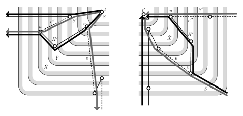
Figure 5: Transformation of $\mathcal{S}$ in the proof of Lemma 9. The left and right panels illustrate the cases of $\hat{X}\in\mathcal{L}(t)$ and $\hat{X}\in\mathcal{L}(t^{\prime})$, respectively, with $t\neq t^{\prime}$. The paths $S$ and $S^{\prime}$ are represented by dark gray lines; the black lines represent the paths obtained by modifying $S$ and $S^{\prime}$.

Suppose that $\hat{X}\in\mathcal{L}(t)$. Let $\hat{X}$ be the minimal biset such that $\hat{X}\in\mathcal{L}(t)$ and $u\in X^{+}$, and let $\hat{Y}$ be the child of $\hat{X}$. Then, $e^{\prime}\in\delta(\hat{Y})$, and $u\in X^{+}\setminus Y^{+}$. Moreover, another half-integral edge $e^{\prime\prime}\in\delta_{H}(\hat{Y})$, labeled “$-$,” is incident to $u$. Edge $e^{\prime\prime}$ is included in another path $S^{\prime}\in\mathcal{S}$. Let $t^{\prime}$ be the terminal such that $t\neq t^{\prime}$ and $S^{\prime}\in\mathcal{S}_{t^{\prime}}$. After reaching $u$, we move to $t^{\prime}$ along the path $S^{\prime}$. In other words, path $S$ is replaced by the concatenate of $S[t,v]$, $H^{\prime}$, and $S^{\prime}[u,t^{\prime}]$. If $S^{\prime}[u,t^{\prime}]$ contains a half-integral edge labeled by “$-$”, we modified it recursively. These definitions are illustrated in the left panel of Figure 5. Let us observe that this modification does not violate the capacity constraints when the edges are capacitated by $\bar{x}^{*}+x^{\prime}$. Assumption 3 indicates that exactly two half-integral edges are incident to each inner node on $H^{\prime}$. The capacity of each edge on $H^{\prime}$ increases by $1/2$ by the modification, exactly counterbalancing the unused half capacity of each inner node on $H^{\prime}$ prior to the modification. Even if the capacities of edges and nodes on $S^{\prime}[u,t^{\prime}]$ are used before the modification, the flow along $S^{\prime}$ is modified so that these capacities are unused. Thus the capacity constraints are preserved by the modification.

Next, suppose that $\hat{X}\in\mathcal{L}(t^{\prime})$ for some $t^{\prime}$ with $t\neq t^{\prime}$. We first consider the case of $t^{\prime}\neq t_{1}$. Lemma 2(ii) indicates that we can assume $u\in X$. We let $\hat{X}$ be the minimal among such bisets. Another half-integral edge $e^{\prime\prime}\in\delta(\hat{X})$, labeled by “$-$,” is incident to $u$, and is included in a path in $\{R_{1}^{t^{\prime}},\ldots,R_{2r(t^{\prime})}^{t^{\prime}}\}$. Without loss of generality, we suppose that that $R_{1}^{t^{\prime}}$ is such a path. After arriving at $u$, we reach $t^{\prime}$ along $R_{1}^{t^{\prime}}[u,t^{\prime}]$, as shown in the right panel of Figure 5. Again, this modification preserves the capacity constraints. To see this, suppose that another path $S^{\prime}\in\mathcal{S}\setminus\{S\}$ includes $R_{1}^{t^{\prime}}$. Then, $S^{\prime}$ includes a “$-$”-labeled edge before reaching $u$ when traversed from $t$ to $t^{\prime}$. $S^{\prime}$ will be diverted to another route, and half of the edge and node capacity on $R_{1}^{t^{\prime}}[u,t^{\prime}]$ will be no longer used. Prior to modification, half of the inner node capacity of $H^{\prime}$ was unused because the nodes were incident to exactly two half-integral edges.

We next discuss the case of $t^{\prime}=t_{1}$. In this case, $t\in\{t_{2},t_{k}\}$. Recall that all edges in $H_{1}$ are labeled by “$+$.” Each of $H_{2}$ and $H_{k}$ shares exactly one edge with $H_{1}$. We let $e_{1}$ denote the edge shared by $H_{1}$ and $H_{k}$, and $e_{2}$ denote the one shared by $H_{1}$ and $H_{2}$. $e_{1}$ and $e_{2}$ are traversed inward and outward with respect to $t_{1}$, respectively. If $t=t_{2}$, we modify each path in $\mathcal{S}_{t_{1}}$ as when each outward-traversed edge in $H_{1}$ is labeled “$-$,” whereas other edges are labeled “$+$.” If $t=t_{k}$, we perform the converse operation, implemented when each outward-traversed edge in $H_{1}$ is labeled “$+$,” whereas other edges are labeled “$-$.” The modification when $t=t_{2}$ is illustrated in Figure 6. Recall that we chosen $t_{1}$ so that $t_{2}\neq t_{k}$. The capacity constraints are preserved because no path in $\mathcal{S}$ includes $e_{1}$ when $t=t_{2}$, and no path in $\mathcal{S}$ includes $e_{2}$ if $t=t_{k}$ before the modification.

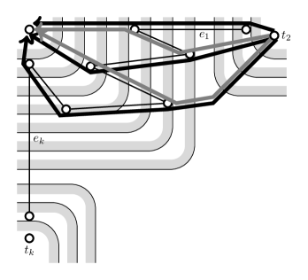
Figure 6: Modification of $\mathcal{S}$ when $t=t_{2}$. Gray thick lines represent paths before the modification, and black lines represent those after the modification.

These transformations generate a flow of amount $r(t)$ from $t$ to $T\setminus\{t\}$ in the graph capacitated by $\bar{x}^{*}+x^{\prime}$. This indicates that $x^{\prime}\in P(f^{\kappa}_{\bar{x}^{*}},\mathbf{1})$. Assigning unbounded capacity to each node in $V\setminus T$, a similar proof can be derived for $h=f^{\lambda}$. ∎

5 Relationship between terminal backup and multiflow

In this section, we limit the constraints on the generalized terminal backup problem to the edge-connectivity constraints, unless otherwise stated. Furthermore, our discussion of multiflows assumes that edges alone are capacitated. Let $\mathcal{A}$ denote the set of paths connecting distinct terminals, and assume that the capacity constraints and flow demands are satisfied by a multiflow $\psi\colon\mathcal{A}\rightarrow\mathbb{Q}_{+}$, i.e., $\sum_{A\in\mathcal{A}\colon e\in E(A)}\psi(A)\leq u(e)$ for each $e\in E$ and $\sum_{A\in\mathcal{A}_{t}}\psi(A)\geq r(t)$ for each $t\in T$. We call a vector (or a function) $1/k$-fractional if each entry multiplied by $k$ is an integer.

In this section, we answer the question: to what extent the edge-connectivity terminal backup differs from the minimum cost multiflow problem in the edge-capacitated setting? The differences are small, as demonstrated below.

Lemma 10.

For each $1/k$-fractional multiflow, there exists a $1/k$-fractional vector of the same cost in $P(f^{\lambda},u)$. For each $1/2k$-fractional vector $x$, where $x$ is minimal in $P(f^{\lambda},u)$ and $x(\delta(v))$ is $1/k$-fractional for each $v\in V\setminus T$, there exists a $1/2k$-fractional multiflow $\psi$ such that $x(e)=\sum_{A\in\mathcal{A}\colon e\in E(A)}\psi(A)$.

The former part of Lemma 10 is straightforward to prove; if $\psi$ is a $1/k$-fractional multiflow, then $x\colon E\rightarrow\mathbb{Q}_{+}$ defined by $x(e)=\sum_{A\in\mathcal{A}\colon e\in E(A)}\psi(A)$ is $1/k$-fractional and belongs to $P(f^{\lambda},u)$.

To prove the latter part, we use a graph operation called splitting off. Let $e=uv$ and $e^{\prime}=u^{\prime}v$ be two edges incident to the same node $v$. Splitting off $e$ and $e^{\prime}$ replaces both $e$ and $e^{\prime}$ by a new edge $uu^{\prime}$. In this section, we regard $f^{\lambda}$ as a set function. To avoid confusion, we denote $f^{\lambda}$ defined from $r\colon T\rightarrow\mathbb{Z}_{+}$ by $f^{\lambda}_{r}$. Let $J$ be an edge set on $V$ such that

$$|\delta_{J}(X)|\geq f^{\lambda}_{r}(X)\text{ for each }X\in 2^{V}.$$ (4)

We say that a pair of edges in $J$ incident to the same node is admissible (with respect to $f^{\lambda}_{r}$) when (4) holds after splitting off the edges.

Lemma 11.

Let $J$ be an edge set on $V$ that satisfies (4), and let $v$ be a node in $V\setminus T$ with $|\delta_{J}(v)|\neq 3$. Then $\delta_{J}(v)$ includes an admissible pair with respect to $f^{\lambda}_{r}$ or (4) holds even after an edge is removed from $\delta_{J}(v)$.

Lemma 11 derives from a theorem in [15, 3], which gave a condition for admissible pairs in a more general setting. Bernáth and Kobayashi [4] proved an almost identical claim when discussing the degree-specified version of the edge-connectivity terminal backup, but did not explicitly specify the condition under which admissible pairs can exist. For completeness, we provide a proof of Lemma 11 in Appendix A.

Proof of Lemma 10. The former part of Lemma 10 has been proven above. Here, we concentrate on the latter part. Since $x$ is $1/2k$-fractional, $2kx(e)\in\mathbb{Z}_{+}$ for each $e\in E$. Let $J$ be the set of $2kx(e)$ edges parallel to $e$ for each $e\in E$. Since $x(\delta(X))\geq f^{\lambda}_{r}(X)$ for each $X\in 2^{V}$, $J$ satisfies

$$|\delta_{J}(X)|\geq 2kf^{\lambda}_{r}(X)=f^{\lambda}_{2kr}(X)\text{ for each }X\in 2^{V}.$$ (5)

Let $v\in V\setminus T$. Since $x(\delta(v))$ is $1/k$-fractional, $|\delta_{J}(v)|$ is an even integer. By the minimality of $x$, no edge can be removed from $\delta_{J}(v)$ without violating (5). Hence, by Lemma 11, $\delta_{J}(v)$ includes an admissible pair with respect to $f^{\lambda}_{2kr}$. For each $v\in V\setminus T$, we repeatedly split off admissible pairs of edges incident to $v$ until no edge is incident to $v$. The graph at the end of this process is denoted by $(V,J^{\prime})$. In $J^{\prime}$, no edge is incident to nodes in $V\setminus T$, and at least $2kr(t)$ edges join $t\in T$ to other terminals. An edge joining terminals $t$ and $t^{\prime}$ in $J^{\prime}$ is generated by splitting off edges on a path between $t$ and $t^{\prime}$ in $J$. In other words, edges in $J^{\prime}$ correspond to edge-disjoint $T$-paths in $J$. By pushing a $1/2k$ unit of flow along each of these $T$-paths in $G$, we obtain the required multiflow.

We see that Theorem 2 follows from Lemma 10 and the properties of $P(f^{\lambda},u)$ described in Section 3.

Proof of Theorem 2. The former part of Lemma 10 implies that $\mathsf{LP}(f^{\lambda},u)$ relaxes the minimum cost multiflow problem. As proven in Corollary 1, $\mathsf{LP}(f^{\lambda},u)$ admits a half-integral optimal solution $x$. This solution can be computed in strongly polynomial time and is guaranteed minimal in $P(f^{\lambda},u)$, as shown in Section 4. By Lemma 3, $x(\delta(v))$ is integer-valued for each $v\in V$. Hence, the latter part of Lemma 10 implies that there exists a half-integral multiflow $\psi$ such that $x(e)=\sum_{A\in\mathcal{A}:e\in E(A)}\psi(A)$. Note that $\sum_{e\in E}c(e)x(e)=\sum_{A\in\mathcal{A}}c(A)\psi(A)$, and therefore $\psi$ minimizes the cost among all feasible multiflows.

How $\psi$ should be computed from $x$ in strongly polynomial time is unknown. However, because $\sum_{A\in\mathcal{A}_{t}}\psi(A)=x(\delta(t))$, $\nu(t)=\sum_{A\in\mathcal{A}_{t}}\psi(A)$ can be computed for each $t\in T$. Moreover, $\nu(t)$ is an integer for each $t\in T$. Therefore, as explained in Section 1.2, this problem reduces to minimizing the cost of maximum multiflow, for which a strongly polynomial-time algorithm is known [13].

Each vector $x\in P(f^{\kappa},u)$ belongs to $P(f^{\lambda},u)$. Hence, we can show that each minimal extreme point of $P(f^{\kappa},u)$ admits a half-integral multiflow of the same cost which is feasible in the edge-capacitated setting. However we cannot relate extreme points of $P(f^{\kappa},u)$ to feasible multiflows in the node-capacitated setting as we observed for star graphs in Section 1.2.

6 Conclusion

We have presented $4/3$-approximation algorithms for the generalized terminal backup problem. Our result also implies that the integrality gaps of the LP relaxations are at most $4/3$. These gaps are tight even in the edge cover problem (i.e., $T=V$ and $r\equiv 1$): Consider an instance in which $G$ is a triangle with unit edge costs; The half-integral solution $x$ with $x(e)=1/2$ for all $e\in E$ is feasible to the LPs, and its cost is $3/2$; On the other hand, any integer solution chooses at least two edges from the triangle; Since the costs of these integer solutions are at least $2$, the integrality gap is not smaller than $4/3$ in this instance.

An obvious open problem is whether the generalized terminal backup problem admits polynomial-time exact algorithms or not. It seems hard to obtain such an algorithm by rounding solutions of the LP relaxations because of their integrality gaps. For the capacitated $b$-edge cover problem, an LP relaxation of integrality gap one is known [16]. For obtaining an LP-based polynomial-time algorithm for the generalized terminal backup problem, we have to extend this LP relaxation for the capacitated $b$-edge cover problem.

Another interesting approach is offered by combinatorial approximation algorithms because it is currently a major open problem to find a combinatorial constant-factor approximation algorithm for the survivable network design problem, for which the Jain’s iterative rounding algorithm [11] achieves 2-approximation. The survivable network design problem involves more complicated connectivity constraints than the generalized terminal backup problem. Hence, study on combinatorial algorithms for the latter problem may give useful insights for the former problem. Recently, Hirai [10] showed that $\mathsf{LP}(f^{\lambda},u)$ can be solved by a combinatorial algorithm. Indeed, he also showed that his algorithm can be used to implement our $4/3$-approximation algorithm for the edge-connectivity terminal backup without generic LP solvers.

Many problems related to multiflows also remain open. We have shown that an LP solution provides a minimum cost half-integral multiflow that satisfies the flow demand from each terminal in the edge-capacitated setting. However, how the computation should proceed in the node-capacitated setting remains elusive. Computing a minimum cost integral multiflow under the same constraints is yet another problem worth investigating. We note that Burlet and Karzanov [5] solved a similar problem related to integral multiflows in the edge-capacitated setting. Their problem differs from ours in the fact that $\sum_{A\in\mathcal{A}_{t}}\psi(A)$ is required to match the specified value for each terminal $t$.

Appendix A Proof of Lemma 11

Since Lemma 11 is trivial when $|\delta_{J}(v)|\leq 2$, we here suppose that $|\delta_{J}(v)|\geq 4$. Assuming that no edge in $\delta_{J}(v)$ can be removed without violating (4), we prove that an admissible pair exists in $\delta_{J}(v)$.

We denote $V\setminus\{v\}$ by $V^{\prime}$, $\delta_{J}(v)$ by $A$, and $J\setminus A$ by $J^{\prime}$. For each $X\in 2^{V^{\prime}}$, we let $\bar{X}$ denote $V^{\prime}\setminus X$, and define $p(X)$ as $\max\{f^{\lambda}_{r}(X),f^{\lambda}_{r}(\bar{X})\}-|\delta_{J^{\prime}}(X)|$. Note that $p$ is a symmetric skew supermodular function on $2^{V^{\prime}}$. $J$ satisfies (4) if and only if $|\delta_{A}(X)|\geq p(X)$ for each $X\in 2^{V^{\prime}}$. The assumption implies that each $e\in A$ is incident to some $X\in 2^{V^{\prime}}$ such that $|\delta_{A}(X)|=p(X)>0$. A pair of $uv,u^{\prime}v\in A$ is admissible if and only if no $X\in 2^{V^{\prime}}$ satisfies $u,u^{\prime}\in X$ and $|\delta_{A}(X)|\leq 1+p(X)$. We call $X\in 2^{V^{\prime}}$ a dangerous set when $2\leq|\delta_{A}(X)|\leq 1+p(X)$.

If $X$ is a dangerous set, then $p(X)\geq 1$. Since $p(X)\geq 1$ implies $f^{\lambda}_{r}(X)\geq 1$ or $f^{\lambda}_{r}(\bar{X})\geq 1$, we have $|X\cap T|=1$ or $|\bar{X}\cap T|=1$ for such $X$. Without loss of generality, we assume that each $t\in T$ admits $X\in 2^{V^{\prime}}$ with $t\in X$ and $p(X)>0$ (otherwise, it suffices to prove the lemma after removing $t$ from $T$). We denote $\{X\in 2^{V^{\prime}}\colon X\cap T=\{t\}\}$ by $\mathcal{C}^{\prime}(t)$, and the set of $X\in\mathcal{C}^{\prime}(t)$ attaining $\min_{X\in\mathcal{C}^{\prime}(t)}|\delta_{J^{\prime}}(X)|$ by $\mathcal{M}(t)$. Since $\max\{f^{\lambda}_{r}(X),f^{\lambda}_{r}(\bar{X})\}=r(t)$ for all $X\in\mathcal{C}^{\prime}(t)$, we have $p(Y)\geq 1$ for each $Y\in\mathcal{M}(t)$. Since $J$ satisfies (4), $|\delta_{A}(Y)|\geq 1$ for each $Y\in\mathcal{M}(t)$.

Lemma 12.

Let $t,t^{\prime}\in T$ with $t\neq t^{\prime}$.

• If $X,Y\in\mathcal{M}(t)$, then $X\cap Y,X\cup Y\in\mathcal{M}(t)$.

• If $X\in\mathcal{M}(t)$ and $Y\in\mathcal{M}(t^{\prime})$, then $X\setminus Y\in\mathcal{M}(t)$ and $Y\setminus X\in\mathcal{M}(t^{\prime})$.

• If $X$ is minimal in $\mathcal{M}(t)$ and $Y\in\mathcal{M}(t^{\prime})$, then $X\cap Y=\emptyset$.

Proof.

It is known that $|\delta_{J^{\prime}}(X)|+|\delta_{J^{\prime}}(Y)|\geq|\delta_{J^{\prime}}(X\cap Y)|+|\delta_{J^{\prime}}(X\cup Y)|$ and $|\delta_{J^{\prime}}(X)|+|\delta_{J^{\prime}}(Y)|\geq|\delta_{J^{\prime}}(X\setminus Y)|+|\delta_{J^{\prime}}(Y\setminus X)|$ hold for any $X,Y\in 2^{V^{\prime}}$. If $X,Y\in\mathcal{M}(t)$, then $f^{\lambda}_{r}(X)=f^{\lambda}_{r}(Y)=f^{\lambda}_{r}(X\cap Y)=f^{\lambda}_{r}(X\cup Y)=r(t)$. If $X\in\mathcal{M}(t)$ and $Y\in\mathcal{M}(t^{\prime})$ with $t\neq t^{\prime}$, then $f^{\lambda}_{r}(X)=f^{\lambda}_{r}(X\setminus Y)=r(t)$ and $f^{\lambda}_{r}(Y)=f^{\lambda}_{r}(Y\setminus X)=r(t^{\prime})$. (i) and (ii) follow from these properties. (iii) is indicated by (ii). ∎

(i) implies that a minimal node set and a maximal node set in $\mathcal{M}(t)$ are unique. We denote the minimal node set in $\mathcal{M}(t)$ by $Z_{t}$, and the maximal node set in $\mathcal{M}(t)$ by $W_{t}$.

In previous work [15, 3], it was shown that $A$ includes an admissible pair if $p(X)\geq 2$ holds for some $X\in 2^{V^{\prime}}$. Hence, in the following discussion, we assume that $p(X)\leq 1$ for each $X\in 2^{V^{\prime}}$. By this assumption, $p(X)=1$ holds if and only if $X\in\bigcup_{t\in T}\mathcal{M}(t)$. Moreover, $X$ is a dangerous set if and only if $|\delta_{A}(X)|=2$, and $X$ or $\bar{X}$ belongs to $\bigcup_{t\in T}\mathcal{M}(t)$.

First, let us prove by contradiction that $|T|\geq 4$. For this purpose, we suppose that $|T|\leq 3$. As mentioned above, for each $e\in A$, there exists $X\in 2^{V^{\prime}}$ such that $\delta_{A}(X)=\{e\}$, and $X\in\bigcup_{t\in T}\mathcal{M}(t)$ or $\bar{X}\in\bigcup_{t\in T}\mathcal{M}(t)$ holds. We let $X_{e}$ denote one of such $X$. Because $|A|\geq 4$, there exist $t\in T$ and distinct edges $e,g\in A$ such that $X_{e}\in\mathcal{M}(t)$ or $\bar{X}_{e}\in\mathcal{M}(t)$, and $X_{g}\in\mathcal{M}(t)$ or $\bar{X}_{g}\in\mathcal{M}(t)$. If both $X_{e}$ and $X_{g}$ belong to $\mathcal{M}(t)$, then $\delta_{A}(Z_{t})\subseteq\delta_{A}(X_{e})\cap\delta_{A}(X_{g})=\emptyset$. Since this contradicts $|\delta_{A}(Z_{t})|\geq p(Z_{t})=1$, $\bar{X}_{e}\in\mathcal{M}(t)$ or $\bar{X}_{g}\in\mathcal{M}(t)$ holds. Without loss of generality, let $\bar{X}_{e}\in\mathcal{M}(t)$. Then $X_{e}\cap T=T\setminus\{t\}$. Since $\bar{X}_{e}\subseteq W_{t}$, $Z_{t^{\prime}}\subseteq X_{e}$ holds for each $t^{\prime}\in T\setminus\{t\}$. We notice that $\emptyset\neq\delta_{A}(Z_{t^{\prime}})\subseteq\delta_{A}(X_{e})$ holds for each $t^{\prime}\in T\setminus\{t\}$, and $\delta_{A}(Z_{t^{\prime}})\cap\delta_{A}(Z_{t^{\prime\prime}})=\emptyset$ holds for each $t^{\prime},t^{\prime\prime}\in T\setminus\{t\}$ with $t^{\prime}\neq t^{\prime\prime}$. Since these facts imply $|\delta_{A}(X_{e})|\geq 3$, they contradict the definition of $X_{e}$. Therefore $|T|\geq 4$.

Let $t_{1},t_{2}\in T$ with $t_{1}\neq t_{2}$, $e_{1}\in\delta_{A}(Z_{t_{1}})$, and $e_{2}\in\delta_{A}(Z_{t_{2}})$. Suppose that the pair of $e_{1}$ and $e_{2}$ is not admissible. Then, there exists a dangerous set $Y$ with $\delta_{A}(Y)=\{e_{1},e_{2}\}$. $Y\in\mathcal{M}(t_{3})$ or $\bar{Y}\in\mathcal{M}(t_{3})$ for some $t_{3}\in T$. In the former case, if $t_{3}\neq t_{1}$, the existence of $e_{1}\in\delta_{A}(Y)\cap\delta_{A}(Z_{t_{1}})$ contradicts $Y\cap Z_{t_{1}}=\emptyset$, and if $t_{3}=t_{1}$, the existence of $e_{2}\in\delta_{A}(Y)\cap\delta_{A}(Z_{t_{2}})$ contradicts $Y\cap Z_{t_{2}}=\emptyset$. Hence, $\bar{Y}\in\mathcal{M}(t_{3})$. Existence of $e_{1}$ and $e_{2}$ implies that $Z_{t_{1}}\setminus\bar{Y}\neq\emptyset\neq Z_{t_{2}}\setminus\bar{Y}$. If $t_{3}\in\{t_{1},t_{2}\}$, the minimality of $Z_{t_{1}}$ or $Z_{t_{2}}$ is violated. Hence, $t_{3}\not\in\{t_{1},t_{2}\}$. Now, let $t_{4}\in T\setminus\{t_{1},t_{2},t_{3}\}$, and $e_{4}\in\delta_{A}(Z_{t_{4}})$. Since $e_{4}\in A\setminus\delta_{A}(Y)=\delta_{A}(\bar{Y})$, we obtain $\bar{Y}\cap Z_{t_{4}}\neq\emptyset$, which also presents a contradiction.

References

- [1] E. Anshelevich and A. Karagiozova. Terminal backup, 3D matching, and covering cubic graphs. SIAM Journal on Computing, 40(3):678–708, 2011.
- [2] M. A. Babenko and A. V. Karzanov. Min-cost multiflows in node-capacitated undirected networks. Journal of Combinatorial Optimization, 24(3):202–228, 2012.
- [3] A. Bernáth and T. Király. A unifying approach to splitting-off. Combinatorica, 32:373–401, 2012.
- [4] A. Bernáth and Y. Kobayashi. The generalized terminal backup problem. In SODA, pages 1678–1686, 2014.
- [5] M. Burlet and A. V. Karzanov. Minimum weight ()-joins and multi-joins. Discrete Mathematics, 181(1-3):65–76, 1998.
- [6] J. Cheriyan, S. Vempala, and A. Vetta. Network design via iterative rounding of setpair relaxations. Combinatorica, 26:255–275, 2006.
- [7] B. V. Cherkassky. A solution of a problem on multicommodity flows in a network. Ekonomika i Matematicheskie Metody, 13(1):143–151, 1977.
- [8] L. Fleischer, K. Jain, and D. P. Williamson. Iterative rounding 2-approximation algorithms for minimum-cost vertex connectivity problems. Journal of Computer and System Sciences, 72(5):838–867, 2006.
- [9] H. Hirai. Half-integrality of node-capacitated multiflows and tree-shaped facility locations on trees. Mathematical Programming, 137(1-2):503–530, 2013.
- [10] H. Hirai. L-extendable functions and a proximity scaling algorithm for minimum cost multiflow problem. ArXiv e-prints, Nov. 2014.
- [11] K. Jain. A factor 2 approximation algorithm for the generalized Steiner network problem. Combinatorica, 21(1):39–60, 2001.
- [12] A. V. Karzanov. A problem on maximum multifow of minimum cost. Combinatorial Methods for Flow Problems, pages 138–156, 1979. in Russian.
- [13] A. V. Karzanov. Minimum cost multifows in undirected networks. Mathematical Programming, 66(3):313–325, 1994.
- [14] L. Lovász. On some connectivity properties of Eulerian graphs. Acta Mathematica Hungarica, 28(1):129–138, 1976.
- [15] Z. Nutov. Approximating connectivity augmentation problems. ACM Transactions on Algorithms, 6(1):5, 2009.
- [16] A. Schrijver. Combinatorial Optimization – Polyhedra and Efficiency. Springer, 2003.
- [17] E. Tardos. A strongly polynomial algorithm to solve combinatorial linear programs. Operations Research, 34(2):250–256, 1986.