Delay-Exponent of Bilayer Anytime Code

Md. Noor-A-Rahim, Khoa D. Nguyen and Gottfried Lechner This work was supported by the Australian Research Council Grant DE12010016. Institute for Telecommunications Research
University of South Australia
Adelaide, Australia
noomy004@mymail.unisa.edu.au, {khoa.nguyen, gottfried.lechner}@unisa.edu.au
Abstract

In this paper, we study the design and the delay-exponent of anytime codes over a three terminal relay network. We propose a bilayer anytime code based on anytime spatially coupled low-density parity-check (LDPC) codes and investigate the anytime characteristics through density evolution analysis. By using mathematical induction technique, we find analytical expressions of the delay-exponent for the proposed code. Through comparison, we show that the analytical delay-exponent has a close match with the delay-exponent obtained from numerical results.

I Introduction

Anytime transmission was shown to be necessary and sufficient for tracking and controlling an unstable plant over a noisy channel [1]. The necessary requirements of anytime transmission are causal encoding, decoding at any time instant and exponential decay of error probability with the decoding delay. Anytime transmission feasibility for the point-to-point case was first proved with sequential random codes in [2]. However, these codes were not suitable for practical implementation. More recently, practical anytime codes based on LDPC convolutional codes were proposed in [3] and [4].

In contrast to point-to-point anytime transmission, not much work has been done on anytime transmission over relay channels. Theoretical analysis of the delay-exponent for decode-and-forward (DF) relaying and compress-and-forward (CF) relaying were investigated in [5] and [6], respectively. The first practical bilayer anytime codes for DF relaying were shown in our previous work [7]. These bilayer codes offer simple encoding and provide good performance over relay channels. However, due to the multi edge type structure, the density evolution analysis for these bilayer codes is complicated. Moreover, no analysis for the delay-exponent was presented in [7].

The contributions of this work are as follows. We design a new bilayer anytime code for DF relaying which allows tractable analytical analysis. We show the anytime characteristics of the proposed code over binary erasure relay channels through density evolution analysis. We derive an analytical bound for the corresponding delay-exponent using mathematical induction technique and observe a close match with the numerical delay-exponent.

II Preliminaries

II-A Anytime Transmission

Consider a streaming source, where at time $t$, a $K$-bit message $\boldsymbol{m}_{t}\in\{0,1\}^{K}$ is produced. At time instant $t$, the anytime channel encoder produces a $M$-bit channel input $\boldsymbol{u}_{t}\in\{0,1\}^{M}$ as a function of the available source information $\boldsymbol{m}_{1}^{t}=[\boldsymbol{m}_{1},\boldsymbol{m}_{2},....,\boldsymbol{m}_{t}]$. We define the anytime channel encoder by the function $E_{t}(\boldsymbol{m}_{1}^{t})$. The encoded message $\boldsymbol{u}_{t}$ is then transmitted over a noisy channel. The anytime channel decoder receives $\boldsymbol{v}_{t}$ (noisy version of $\boldsymbol{u}_{t}$) at every time step $t$. The decoder estimates the transmitted messages using the decoding function $\boldsymbol{\hat{m}}_{1}^{t}(t)=D_{t}(\boldsymbol{v}_{1}^{t})$, i.e., the decoder produces an estimate $\boldsymbol{\hat{m}}_{1}^{t}(t)$ based on the current as well as all previously received messages.

We now consider the estimate $\boldsymbol{\hat{m}}_{i}(t)$ of message $\boldsymbol{m}_{i}$ at time $t\geq i$ ; the corresponding decoding delay for message $\boldsymbol{m}_{i}$ is $d=t-i$. The probability of error for the message $i$ at time $t$ will be Pe​(i,t)=Pr⁑(π’Ž^i​(t)β‰ π’Ži)subscript𝑃𝑒𝑖𝑑Prsubscriptbold-^π’Žπ‘–π‘‘subscriptπ’Žπ‘–P_{e}(i,t)=\Pr\left(\boldsymbol{\hat{m}}_{i}(t)\neq\boldsymbol{m}_{i}\right). For a given channel, the encoder-decoder pair $(E_{t},D_{t})$ is called anytime code if there exists a finite $\beta>0$ such that [8]:

$$P_{e}(i,t)\leq\beta e^{-\alpha(t-i)},\hskip 5.69046pt\forall\hskip 2.84544pt(t-i)\geq 0,$$ (1)

where $\alpha>0$ is known as delay-exponent. The delay-exponent $\alpha$ specifies how fast the reliability of the system improves with the delay. The inequality in (1) is the major property of an anytime code. (1) implies that at any delay $d\geq 0$, the decoder is capable of estimating the message $\boldsymbol{m}_{i}$ and the probability of error for that message will decay exponentially to zero as the delay $d$ approaches infinity.

II-B Anytime Spatially Coupled LDPC Codes

Anytime spatially coupled LDPC [4] codes are constructed by coupling an infinite number of standard $(d_{v},d_{c})$-regular LDPC protographs, where $d_{v}$ and $d_{c}$ are the degrees of variable nodes and check nodes, respectively. We assume that each protograph/position contains $M$ variables and $\frac{d_{v}}{d_{c}}M$ check nodes. To ensure causal streaming and anytime decoding capability, each of the $d_{v}$ edges of a variable node at position $i$ is connected to a check node $j$ independently chosen from the range range $[i,i+1,...,i+\infty]$. The check node $j$ is chosen such that $j-i$ follows an exponential distribution and hence, a variable node at position $i$ has more connections with the check nodes close to position $i$. Particularly, the probability an edge originated from a variable node (VN) at position $i$ connects to a check node (CN) at position $j$ $(j\geq i)$ is

$\displaystyle P_{r}(k)=e^{-k\lambda}(1-e^{-\lambda}),$ (2)

where $0<\lambda<1$ is known as exponential rate parameter and $k=j-i$ is the distance between the connected check node and variable node. In this paper, we refer to the above mentioned code as $(d_{v},d_{c},\lambda)$-anytime SC-LDPC code.

We consider $M$ to be the number of variable nodes at each position which represent a single message. We also consider $t$ as the number of messages received so far. For the density evolution of the above $(d_{v},d_{c},\lambda)$-anytime SCLDPC codes, we assume an infinite number of variable nodes $(M=\infty)$ at each position. Let $x^{(l)}(i,t)$ be the erasure probability of a message outgoing from a VN at position $i$ in the $l^{th}$ iteration at time $t$. For any $t\geq i$, we get the following density evolution equation for the $(d_{v},d_{c},\lambda)$-anytime SCLDPC code,

$\displaystyle x^{(l)}(i,t)=$ $\displaystyle\epsilon\left(1-\sum\limits_{j=0}^{t-i}P_{r}(j)\bigg{(}1-\right.$
$\displaystyle\left.\sum\limits_{k=0}^{\infty}P_{r}(k)x^{(l-1)}(i+j-k,t)\bigg{)}^{d_{c}-1}\right)^{d_{v}-1},$ (3)

where $\epsilon$ is the channel erasure probability and

$\displaystyle x^{(0)}(i,t)=\begin{cases}0&\text{if}\hskip 5.69046pti\leq 0\\ \epsilon&\text{if}\hskip 5.69046pt0<i\leq t\\ 1&\text{if}\hskip 5.69046pti>t\end{cases}$

II-C Relay Channel and Bilayer Codes

In this paper, we consider three terminal relay networks, which consist of a source, a relay and a destination. The communication links/channels of this system are: source-relay s​rπ‘ π‘Ÿsr, relay-destination $rd$ and source-destination $sd$. We assume that all three links are binary erasure channels and are mutually orthogonal. Let Ο΅s​rsubscriptitalic-Ο΅π‘ π‘Ÿ\epsilon_{sr}, $\epsilon_{rd}$ and $\epsilon_{sd}$ denote the erasure probabilities of the three channels respectively. As a relaying protocol, we consider the decode-and-forward strategy.

With a bilayer coding scheme [9], the source first encodes the information bits using a code π’žs​rsubscriptπ’žπ‘ π‘Ÿ\mathcal{C}_{sr} and then transmits the encoded bits. We assume that the relay can decode the message correctly. However, the destination is unable to recover the encoded bits received from the source due to the bad channel quality of the source-destination link. The relay generates extra parity bits based on the received bits using a code $\mathcal{C}_{r}$. These extra parity bits are then encoded using another code $\mathcal{C}_{rd}$ and sent to destination. The destination recovers the source message with the help of the extra parity information received from the relay.

III Proposed Bilayer Anytime SC-LDPC Code

III-A Code design

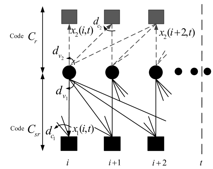
We design the bilayer anytime codes for relay channels according to the bilayer coding scheme described in [9] and [10]. The source causally encodes the messages by using a $(d_{v_{1}},d_{c_{1}},\lambda_{1})$-anytime SC-LDPC code π’žs​rsubscriptπ’žπ‘ π‘Ÿ\mathcal{C}_{sr} and broadcasts the encoded messages to the relay and destination. Due to the anytime characteristics of code π’žs​rsubscriptπ’žπ‘ π‘Ÿ\mathcal{C}_{sr}, the relay has to wait for a certain number of messages to receive for successful recovery of the source bits. However, in this work, we ignore this initial delay required at the relay and hence we assume error-free transmission from the source to the relay. Based on the received messages, the relay causally generates extra parity bits using another $(d_{v_{2}},d_{c_{2}},\lambda_{2})$-anytime SC-LDPC code $\mathcal{C}_{r}$. Then the relay encodes these extra parity bits using a capacity approaching111 We refer to a code as capacity approaching code, when the rate of the code approaches the capacity of the corresponding channel. For BEC, the capacity of the channel $i$ is $C_{i}=1-\epsilon_{i}$, where $\epsilon_{i}$ is the erasure probability of channel $i$. block code for the relay destination link, which ensures secure transmission of relaying bits to the destination. The destination first decodes the extra parity bits from the relay and uses them as side information to decode the information received from the source. We refer to the combination of the code π’žs​rsubscriptπ’žπ‘ π‘Ÿ\mathcal{C}_{sr} and the code $\mathcal{C}_{r}$ as $(d_{v_{1}},d_{c_{1}},\lambda_{1},d_{v_{2}},d_{c_{2}},\lambda_{2})$-bilayer anytime SC-LDPC code. Such a bilayer anytime code is depicted in Fig.Β 1.

Refer to caption
Figure 1: $(d_{v_{1}},d_{c_{1}},\lambda_{1},d_{v_{2}},d_{c_{2}},\lambda_{2})$-Bilayer anytime SC-LDPC code

III-B Density Evolution

Now we consider density evolution for the proposed bilayer anytime code. Let $x_{1}^{(l)}(i,t)$ be the erasure probability of a message outgoing from a VN at position $i$ to the CNs of code π’žs​rsubscriptπ’žπ‘ π‘Ÿ\mathcal{C}_{sr} in the $l^{th}$ iteration, at time $t$. Let $x_{2}^{(l)}(i,t)$ be the erasure probability of a message outgoing from a VN at position $i$ to the CNs of code $\mathcal{C}_{r}$ in the $l^{th}$ iteration, at time $t$. We also consider $P_{r_{1}}(k)=e^{-k\lambda_{1}}(1-e^{-\lambda_{1}})$ and $P_{r_{2}}(k)=e^{-k\lambda_{2}}(1-e^{-\lambda_{2}})$. At iteration $l$, we get the following update equations for $x_{1}^{(l)}(i,t)$ and $x_{2}^{(l)}(i,t)$:

$\displaystyle x_{1}^{(l)}(i,t)=\epsilon_{sd}\left(1-\sum\limits_{j=0}^{t-i}P_{r_{1}}(j)\Bigg{(}1-\sum\limits_{k=0}^{\infty}P_{r_{1}}(k)\right.$
$\displaystyle\hskip 2.84544pt.\;\left.x^{(l-1)}_{1}(i+j-k,t)\Bigg{)}^{d_{c_{1}}-1}\right)^{d_{v_{1}}-1}\left(1-\sum\limits_{j=0}^{t-i}P_{r_{2}}(j)\right.$
$\displaystyle\hskip 5.69046pt.\;\Bigg{(}1-\left.\sum\limits_{k=0}^{\infty}P_{r_{2}}(k)x^{(l-1)}_{2}(i+j-k,t)\Bigg{)}^{d_{c_{2}}-1}\right)^{d_{v}{{}_{2}}},$ (4)
$\displaystyle x_{2}^{(l)}(i,t)=\epsilon_{sd}\left(1-\sum\limits_{j=0}^{t-i}P_{r_{1}}(j)\Bigg{(}1-\sum\limits_{k=0}^{\infty}P_{r_{1}}(k)\right.$
$\displaystyle\hskip 2.84544pt.\;\left.x^{(l-1)}_{1}(i+j-k,t)\Bigg{)}^{d_{c_{1}}-1}\right)^{d_{v_{1}}}\left(1-\sum\limits_{j=0}^{t-i}P_{r_{2}}(j)\right.$
$\displaystyle\hskip 5.69046pt.\;\Bigg{(}1-\left.\sum\limits_{k=0}^{\infty}P_{r_{2}}(k)x^{(l-1)}_{2}(i+j-k,t)\Bigg{)}^{d_{c_{2}}-1}\right)^{d_{v}{{}_{2}}-1},$ (5)

where

$\displaystyle x_{1}^{(0)}(i,t)=x_{2}^{(0)}(i,t)=\begin{cases}0&\text{if}\hskip 5.69046pti\leq 0\\ \epsilon_{sd}&\text{if}\hskip 5.69046pt0<i\leq t\\ 1&\text{if}\hskip 5.69046pti>t\end{cases}$

The probability that VN $i$ has been erased can be computed by considering all the edges connected to VN $i$. Thus, the erasure probability $P_{e}(i,t)$ of message $i$ at decoding time instant $t$ is given by:

$\displaystyle P_{e}(i,t)=\epsilon_{sd}\left(1-\sum\limits_{j=0}^{t-i}P_{r_{1}}(j)\Bigg{(}1-\sum\limits_{k=0}^{\infty}P_{r_{1}}(k)\right.$
$\displaystyle\hskip 2.84544pt.\;\left.x^{(\infty)}_{1}(i+j-k,t)\Bigg{)}^{d_{c_{1}}-1}\right)^{d_{v_{1}}}\left(1-\sum\limits_{j=0}^{t-i}P_{r_{2}}(j)\right.$
$\displaystyle\hskip 5.69046pt.\;\Bigg{(}1-\left.\sum\limits_{k=0}^{\infty}P_{r_{2}}(k)x^{(\infty)}_{2}(i+j-k,t)\Bigg{)}^{d_{c_{2}}-1}\right)^{d_{v}{{}_{2}}},$ (6)
Refer to caption
Figure 2: Asymptotic performance of the proposed bilayer anytime code over binary erasure channel ($\epsilon_{sd}=0.7$).

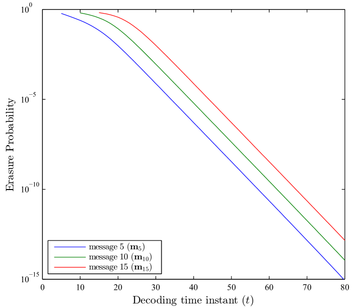
We present the results from the above density evolution analysis. We consider a $(d_{v_{1}},d_{c_{1}},\lambda_{1},d_{v_{2}},d_{c_{2}},\lambda_{2})=(3,6,0.1,2,8,0.1)$-bilayer anytime code. Fig.Β 2 shows the erasure probabilities of three messages versus the decoding time instant. For each of the messages, we observe an exponential decaying of the erasure probability and the erasure performance of a given block is the shifted version of another. This shows that the error performance of a message is only dependent on the decoding delay and is independent on its position. From the erasure probability performance shown in Fig.Β 2, numerically the delay-exponent $\alpha$ can be determined.

III-C Delay-Exponent Analysis

The following theorem gives an analytical formula for the delay exponent.

Theorem 1

Consider the $(d_{v_{1}},d_{c_{1}},\lambda_{1},d_{v_{2}},d_{c_{2}},\lambda_{2})$-bilayer anytime SC-LDPC code described in SubsectionΒ III-A. For a source-destination channel erasure probability below a threshold $\bar{\epsilon}_{sd}$, asymptotically (i.e., for $M=\infty$) the delay-exponent of the proposed bilayer code is given by:

$\displaystyle\alpha=\lambda_{1}d_{v_{1}}+\lambda_{2}d_{v_{2}},$ (7)

where the threshold $\bar{\epsilon}_{sd}$ is defined by:

$\displaystyle\bar{\epsilon}_{sd}=\max\limits_{\beta>0}\;\min\limits_{d\geq 0}\;\beta\left(e^{-\lambda_{1}}+K^{\prime}\right)^{-d_{v_{1}}}\left(e^{-\lambda_{2}}+K^{\prime\prime}\right)^{-d_{v_{2}}}$
Refer to caption
Figure 3: Comparison between theoretical and numerical delay-exponents for four cases: (i) $d_{v_{1}}=3,d_{v_{2}}=2,\lambda_{2}=0.1$ (ii) $d_{v_{1}}=3,d_{v_{2}}=3,\lambda_{2}=0.1$ (iii) $d_{v_{1}}=3,d_{v_{2}}=2,\lambda_{2}=0.2$ (iv) $d_{v_{1}}=4,d_{v_{2}}=2,\lambda_{2}=0.1$. For all cases, we consider $d_{c_{1}}=6,d_{c_{2}}=8$.

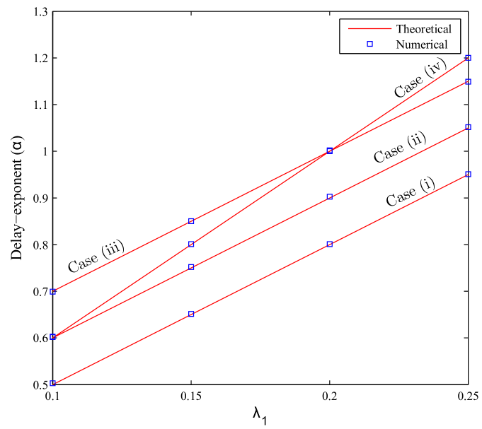
The proof of the theorem and the definitions of $K^{\prime}$ and $K^{\prime\prime}$ are given in the appendix. In Fig.Β 3, we compare the theoretical exponent with the exponent obtained from the numerical results of density evolution. From Fig.Β 3, it is clear that the theoretically determined delay-exponent $\alpha=\lambda_{1}d_{v_{1}}+\lambda_{2}d_{v_{2}}$ closely matches the exponent of the decoded erasure probability obtained from density evolution analysis. We observe that the delay-exponent does not depend on the channel erasure probability $\epsilon_{sd}$ as long as $\epsilon_{sd}$ is below the threshold $\bar{\epsilon}_{sd}$. It is worth mentioning that there exists a large gap between the numerical and the theoretical thresholds due to the approximations taken in the proof of the theorem. For example, with a $(3,6,0.1,2,8,0.1)$-bilayer anytime SC-LDPC code, both the theoretical and numerical delay-exponent is $\alpha=0.5$ while the theoretical and numerical thresholds are $0.115$ and $0.732$, respectively. From (7), we observe that asymptotically the delay-exponent increases linearly with the increment of any parameter ($d_{v_{1}}$, $d_{v_{2}}$, $\lambda_{1}$ and $\lambda_{2}$). However, in practice (i.e., for finite length case), increasing $d_{v_{1}}$ or $d_{v_{2}}$ may introduce short cycles in the code. On the other hand, increasing $\lambda_{1}$ or $\lambda_{2}$ leads to fewer connections to distant protographs. Thus, increasing $d_{v_{1}}$, $d_{v_{2}}$, $\lambda_{1}$ or $\lambda_{2}$ may result in an error floor at large delays.

IV Conclusion

In this paper, we proposed a practical bilayer anytime coding scheme for decode-and-forward relay channel. Through asymptotic analysis, we investigate the anytime characteristics of the proposed code, while ignoring the effect of delays at the source-relay link. For the first time, we have analytically found the delay exponent of a practical code over relay channels and observed a close prediction of the numerical delay-exponent. Our future work will be involved with the analysis of bilayer anytime codes while considering the effect of delays at the source-relay link.

[Proof of TheoremΒ 1] At iteration $l=\infty$, (III-B), (III-B) and (III-B) can be combined as follows:

$\displaystyle x_{e}(i,t)=\epsilon_{sd}\left(1-\sum\limits_{j=0}^{t-i}P_{r_{1}}(j)\Bigg{(}1-\right.$
$\displaystyle\hskip 7.11317pt\;\left.\sum\limits_{k=0}^{\infty}P_{r_{1}}(k)x^{(l-1)}_{1}(i+j-k,t)\Bigg{)}^{d_{c_{1}}-1}\right)^{q_{1}}$
$\displaystyle\hskip 14.22636pt.\;\left(1-\sum\limits_{j=0}^{t-i}P_{r_{2}}(j)\Bigg{(}1-\right.$
$\displaystyle\hskip 21.33955pt\;\left.\sum\limits_{k=0}^{\infty}P_{r_{2}}(k)x^{(l-1)}_{2}(i+j-k,t)\Bigg{)}^{d_{c_{2}}-1}\right)^{q_{2}},$ (8)

where (IV) represents

  • β€’

    (III-B) when $q_{1}=d_{v_{1}}-1$ and $q_{2}=d_{v_{2}}$.

  • β€’

    (III-B) when $q_{1}=d_{v_{1}}$ and $q_{2}=d_{v_{2}}-1$.

  • β€’

    (III-B) when $q_{1}=d_{v_{1}}$ and $q_{2}=d_{v_{2}}$.

By using the following mathematical induction, we find the delay-exponent for the proposed bilayer anytime code.

The basis:

For $0<i\leq d$,

$\displaystyle x_{1}{(t-i,t)}\leq\beta e^{-\alpha_{1}i},\;\text{where}\;\alpha_{1}=\lambda_{1}(d_{v_{1}}-1)+\lambda_{2}d_{v_{2}}$
$\displaystyle x_{2}{(t-i,t)}\leq\beta e^{-\alpha_{2}i},\;\text{where}\;\alpha_{2}=\lambda_{1}d_{v_{1}}+\lambda_{2}(d_{v_{2}}-1)$
$\displaystyle P_{e}{(t-i,t)}\leq\beta e^{-\alpha i},\;\text{where}\;\alpha=\lambda_{1}d_{v_{1}}+\lambda_{2}d_{v_{2}}$
The inductive step:

We have to prove:

$\displaystyle x_{1}{(t-d-1,t)}\leq\beta e^{-\alpha_{1}(d+1)}$ (10a)
$\displaystyle x_{2}{(t-d-1,t)}\leq\beta e^{-\alpha_{2}(d+1)}$ (10b)
$\displaystyle P_{e}{(t-d-1,t)}\leq\beta e^{-\alpha(d+1)}$ (10c)

In the following proof, we consider $K_{1}=e^{-k\lambda_{1}}(1-e^{-\lambda_{1}})=K_{1}e^{-k\lambda_{1}}$ and $P_{r_{2}}(k)=e^{-k\lambda_{2}}(1-e^{-\lambda_{2}})=K_{2}e^{-k\lambda_{2}}$. Note that due to the page limitation, we skip few steps in the following proof. From (IV), we get

xe(tβˆ’dβˆ’1,t)=Ο΅s​d\bBigg@3(1βˆ’βˆ‘j=0d+1Pr1(j)(1βˆ’βˆ‘k=0∞Pr1(k\displaystyle x_{e}(t-d-1,t)=\epsilon_{sd}\bBigg@{3}(1-\sum\limits_{j=0}^{d+1}P_{r_{1}}(j)\Bigg{(}1-\sum\limits_{k=0}^{\infty}P_{r_{1}}(k
.x1(tβˆ’dβˆ’1+jβˆ’k,t))dc1βˆ’1\bBigg@3)q1\bBigg@3(1βˆ’βˆ‘j=0d+1Pr2(j)\displaystyle\hskip 14.22636pt.\;x_{1}(t-d-1+j-k,t)\Bigg{)}^{d_{c_{1}}-1}\bBigg@{3})^{q_{1}}\bBigg@{3}(1-\sum\limits_{j=0}^{d+1}P_{r_{2}}(j)
$\displaystyle\hskip 21.33955pt.\;\left.\left(1-\sum\limits_{k=0}^{\infty}P_{r_{2}}(k)x_{2}(t-d-1+j-k,t)\right)^{d_{c_{2}}-1}\right)^{q_{2}}$
≀(a)Ο΅s​d\bBigg@3(1βˆ’βˆ‘j=0d+1Pr1(j)(1βˆ’Ξ²βˆ‘k=0jβˆ’1Pr1(k)\displaystyle\overset{(a)}{\leq}\epsilon_{sd}\bBigg@{3}(1-\sum\limits_{j=0}^{d+1}P_{r_{1}}(j)\Bigg{(}1-\beta\sum\limits_{k=0}^{j-1}P_{r_{1}}(k)
.eβˆ’Ξ±1​(d+1βˆ’j+k)βˆ’Ξ²βˆ‘k=j∞Pr1(k)eβˆ’Ξ±1​d)dc1βˆ’1\bBigg@3)q1\displaystyle\hskip 14.22636pt.\;e^{-\alpha_{1}(d+1-j+k)}-\beta\sum\limits_{k=j}^{\infty}P_{r_{1}}(k)e^{-\alpha_{1}d}\Bigg{)}^{d_{c_{1}}-1}\bBigg@{3})^{q_{1}}
.\bBigg@3(1βˆ’βˆ‘j=0d+1Pr2(j)(1βˆ’Ξ²βˆ‘k=0jβˆ’1Pr2(k)\displaystyle\hskip 21.33955pt.\;\bBigg@{3}(1-\sum\limits_{j=0}^{d+1}P_{r_{2}}(j)\Bigg{(}1-\beta\sum\limits_{k=0}^{j-1}P_{r_{2}}(k)
.eβˆ’Ξ±2​(d+1βˆ’j+k)βˆ’Ξ²βˆ‘k=j∞Pr2(k)eβˆ’Ξ±2​d)dc2βˆ’1\bBigg@3)q2\displaystyle\hskip 28.45274pt.\;e^{-\alpha_{2}(d+1-j+k)}-\beta\sum\limits_{k=j}^{\infty}P_{r_{2}}(k)e^{-\alpha_{2}d}\Bigg{)}^{d_{c_{2}}-1}\bBigg@{3})^{q_{2}}
=Ο΅s​d\bBigg@3(1βˆ’βˆ‘j=0d+1Pr1(j)(1βˆ’Ξ²K1\displaystyle=\epsilon_{sd}\bBigg@{3}(1-\sum\limits_{j=0}^{d+1}P_{r_{1}}(j)\Bigg{(}1-\beta K_{1}
.βˆ‘k=0jβˆ’1eβˆ’Ξ»1​kβˆ’Ξ±1​(d+1βˆ’j+k)βˆ’Ξ²eβˆ’Ξ»1​jβˆ’Ξ±1​d)dc1βˆ’1\bBigg@3)q1\displaystyle\hskip 14.22636pt.\;\sum\limits_{k=0}^{j-1}e^{-\lambda_{1}k-\alpha_{1}(d+1-j+k)}-\beta e^{-\lambda_{1}j-\alpha_{1}d}\Bigg{)}^{d_{c_{1}}-1}\bBigg@{3})^{q_{1}}
.\bBigg@3(1βˆ’βˆ‘j=0d+1Pr2(j)(1βˆ’Ξ²K2\displaystyle\hskip 21.33955pt.\;\bBigg@{3}(1-\sum\limits_{j=0}^{d+1}P_{r_{2}}(j)\Bigg{(}1-\beta K_{2}
.βˆ‘k=0jβˆ’1eβˆ’Ξ»2​kβˆ’Ξ±2​(d+1βˆ’j+k)βˆ’Ξ²eβˆ’Ξ»2​jβˆ’Ξ±2​d)dc2βˆ’1\bBigg@3)q2\displaystyle\hskip 28.45274pt.\;\sum\limits_{k=0}^{j-1}e^{-\lambda_{2}k-\alpha_{2}(d+1-j+k)}-\beta e^{-\lambda_{2}j-\alpha_{2}d}\Bigg{)}^{d_{c_{2}}-1}\bBigg@{3})^{q_{2}}
=Ο΅s​d\bBigg@3(1βˆ’βˆ‘j=0d+1Pr1(j)(1βˆ’Ξ²K1eβˆ’Ξ±1​(d+1βˆ’j)\displaystyle=\epsilon_{sd}\bBigg@{3}(1-\sum\limits_{j=0}^{d+1}P_{r_{1}}(j)\Bigg{(}1-\beta K_{1}e^{-\alpha_{1}(d+1-j)}
.1βˆ’e(βˆ’Ξ»1βˆ’Ξ±1)​j1βˆ’eβˆ’Ξ»1βˆ’Ξ±1βˆ’Ξ²eβˆ’Ξ»1​jβˆ’Ξ±1​d)dc1βˆ’1\bBigg@3)q1\displaystyle\hskip 14.22636pt.\;\frac{1-e^{(-\lambda_{1}-\alpha_{1})j}}{1-e^{-\lambda_{1}-\alpha_{1}}}-\beta e^{-\lambda_{1}j-\alpha_{1}d}\Bigg{)}^{d_{c_{1}}-1}\bBigg@{3})^{q_{1}}
.\bBigg@3(1βˆ’βˆ‘j=0d+1Pr2(j)(1βˆ’Ξ²K2eβˆ’Ξ±2​(d+1βˆ’j)\displaystyle\hskip 21.33955pt.\;\bBigg@{3}(1-\sum\limits_{j=0}^{d+1}P_{r_{2}}(j)\Bigg{(}1-\beta K_{2}e^{-\alpha_{2}(d+1-j)}
.1βˆ’e(βˆ’Ξ»2βˆ’Ξ±2)​j1βˆ’eβˆ’Ξ»2βˆ’Ξ±2βˆ’Ξ²eβˆ’Ξ»2​jβˆ’Ξ±2​d)dc2βˆ’1\bBigg@3)q2\displaystyle\hskip 28.45274pt.\;\frac{1-e^{(-\lambda_{2}-\alpha_{2})j}}{1-e^{-\lambda_{2}-\alpha_{2}}}-\beta e^{-\lambda_{2}j-\alpha_{2}d}\Bigg{)}^{d_{c_{2}}-1}\bBigg@{3})^{q_{2}}
≀(b)Ο΅s​d\bBigg@3(1βˆ’βˆ‘j=0d+1Pr1(j)(1βˆ’(dc1βˆ’1)(Ξ²K1eβˆ’Ξ±1​(d+1βˆ’j)\displaystyle\overset{(b)}{\leq}\epsilon_{sd}\bBigg@{3}(1-\sum\limits_{j=0}^{d+1}P_{r_{1}}(j)\Bigg{(}1-(d_{c_{1}}-1)\Bigg{(}\beta K_{1}e^{-\alpha_{1}(d+1-j)}
.1βˆ’e(βˆ’Ξ»1βˆ’Ξ±1)​j1βˆ’eβˆ’Ξ»1βˆ’Ξ±1+Ξ²eβˆ’Ξ»1​jβˆ’Ξ±1​d))\bBigg@3)q1\displaystyle\hskip 7.11317pt.\;\frac{1-e^{(-\lambda_{1}-\alpha_{1})j}}{1-e^{-\lambda_{1}-\alpha_{1}}}+\beta e^{-\lambda_{1}j-\alpha_{1}d}\Bigg{)}\Bigg{)}\bBigg@{3})^{q_{1}}
.\bBigg@3(1βˆ’βˆ‘j=0d+1Pr2(j)(1βˆ’(dc2βˆ’1)(Ξ²K2eβˆ’Ξ±2​(d+1βˆ’j)\displaystyle\hskip 14.22636pt.\;\bBigg@{3}(1-\sum\limits_{j=0}^{d+1}P_{r_{2}}(j)\Bigg{(}1-(d_{c_{2}}-1)\Bigg{(}\beta K_{2}e^{-\alpha_{2}(d+1-j)}
.1βˆ’e(βˆ’Ξ»2βˆ’Ξ±2)​j1βˆ’eβˆ’Ξ»2βˆ’Ξ±2+Ξ²eβˆ’Ξ»2​jβˆ’Ξ±2​d))\bBigg@3)q2\displaystyle\hskip 21.33955pt.\;\frac{1-e^{(-\lambda_{2}-\alpha_{2})j}}{1-e^{-\lambda_{2}-\alpha_{2}}}+\beta e^{-\lambda_{2}j-\alpha_{2}d}\Bigg{)}\Bigg{)}\bBigg@{3})^{q_{2}}
=Ο΅s​d\bBigg@3(βˆ‘j=d+2∞Pr1(j)+βˆ‘j=0d+1Pr1(j)(dc1βˆ’1)(Ξ²K1eβˆ’Ξ±1​(d+1βˆ’j)\displaystyle=\epsilon_{sd}\bBigg@{3}(\sum\limits_{j=d+2}^{\infty}P_{r_{1}}(j)+\sum\limits_{j=0}^{d+1}P_{r_{1}}(j)(d_{c_{1}}-1)\Bigg{(}\beta K_{1}e^{-\alpha_{1}(d+1-j)}
.1βˆ’e(βˆ’Ξ»1βˆ’Ξ±1)​j1βˆ’eβˆ’Ξ»1βˆ’Ξ±1+Ξ²eβˆ’Ξ»1​jβˆ’Ξ±1​d)\bBigg@3)q1\displaystyle\hskip 7.11317pt.\;\frac{1-e^{(-\lambda_{1}-\alpha_{1})j}}{1-e^{-\lambda_{1}-\alpha_{1}}}+\beta e^{-\lambda_{1}j-\alpha_{1}d}\Bigg{)}\bBigg@{3})^{q_{1}}
.\bBigg@3(βˆ‘j=d+2∞Pr2(j)+βˆ‘j=0d+1Pr2(j)(dc2βˆ’1)(Ξ²K2eβˆ’Ξ±2​(d+1βˆ’j)\displaystyle\hskip 14.22636pt.\;\bBigg@{3}(\sum\limits_{j=d+2}^{\infty}P_{r_{2}}(j)+\sum\limits_{j=0}^{d+1}P_{r_{2}}(j)(d_{c_{2}}-1)\Bigg{(}\beta K_{2}e^{-\alpha_{2}(d+1-j)}
.1βˆ’e(βˆ’Ξ»2βˆ’Ξ±2)​j1βˆ’eβˆ’Ξ»2βˆ’Ξ±2+Ξ²eβˆ’Ξ»2​jβˆ’Ξ±2​d)\bBigg@3)q2\displaystyle\hskip 21.33955pt.\;\frac{1-e^{(-\lambda_{2}-\alpha_{2})j}}{1-e^{-\lambda_{2}-\alpha_{2}}}+\beta e^{-\lambda_{2}j-\alpha_{2}d}\Bigg{)}\bBigg@{3})^{q_{2}}
=Ο΅s​d\bBigg@3(eβˆ’Ξ»1​(d+2)+βˆ‘j=0d+1K1eβˆ’Ξ»1​j(dc1βˆ’1)(Ξ²K1eβˆ’Ξ±1​(d+1βˆ’j)\displaystyle=\epsilon_{sd}\bBigg@{3}(e^{-\lambda_{1}(d+2)}+\sum\limits_{j=0}^{d+1}K_{1}e^{-\lambda_{1}j}(d_{c_{1}}-1)\Bigg{(}\beta K_{1}e^{-\alpha_{1}(d+1-j)}
.1βˆ’e(βˆ’Ξ»1βˆ’Ξ±1)​j1βˆ’eβˆ’Ξ»1βˆ’Ξ±1+Ξ²eβˆ’Ξ»1​jβˆ’Ξ±1​d)\bBigg@3)q1\displaystyle\hskip 7.11317pt.\;\frac{1-e^{(-\lambda_{1}-\alpha_{1})j}}{1-e^{-\lambda_{1}-\alpha_{1}}}+\beta e^{-\lambda_{1}j-\alpha_{1}d}\Bigg{)}\bBigg@{3})^{q_{1}}
.\bBigg@3(eβˆ’Ξ»2​(d+2)+βˆ‘j=0d+1K2eβˆ’Ξ»2​j(dc2βˆ’1)(Ξ²K2eβˆ’Ξ±2​(d+1βˆ’j)\displaystyle\hskip 14.22636pt.\;\bBigg@{3}(e^{-\lambda_{2}(d+2)}+\sum\limits_{j=0}^{d+1}K_{2}e^{-\lambda_{2}j}(d_{c_{2}}-1)\Bigg{(}\beta K_{2}e^{-\alpha_{2}(d+1-j)}
.1βˆ’e(βˆ’Ξ»2βˆ’Ξ±2)​j1βˆ’eβˆ’Ξ»2βˆ’Ξ±2+Ξ²eβˆ’Ξ»2​jβˆ’Ξ±2​d)\bBigg@3)q2\displaystyle\hskip 21.33955pt.\;\frac{1-e^{(-\lambda_{2}-\alpha_{2})j}}{1-e^{-\lambda_{2}-\alpha_{2}}}+\beta e^{-\lambda_{2}j-\alpha_{2}d}\Bigg{)}\bBigg@{3})^{q_{2}}
=Ο΅s​d\bBigg@3(eβˆ’Ξ»1​(d+2)+eβˆ’Ξ±1​(d+1)(dc1βˆ’1)Ξ²K1\displaystyle=\epsilon_{sd}\bBigg@{3}(e^{-\lambda_{1}(d+2)}+e^{-\alpha_{1}(d+1)}(d_{c_{1}}-1)\beta K_{1}
.\bBigg@3(K11βˆ’eβˆ’Ξ»1βˆ’Ξ±11βˆ’e(βˆ’Ξ»1+Ξ±1)​(d+2)1βˆ’eβˆ’Ξ»1+Ξ±1+\displaystyle\hskip 7.11317pt.\;\bBigg@{3}(\frac{K_{1}}{1-e^{-\lambda_{1}-\alpha_{1}}}\frac{1-e^{(-\lambda_{1}+\alpha_{1})(d+2)}}{1-e^{-\lambda_{1}+\alpha_{1}}}+
(eΞ±1βˆ’K11βˆ’eβˆ’Ξ»1βˆ’Ξ±1)1βˆ’eβˆ’2​λ1​(d+2)1βˆ’eβˆ’2​λ1\bBigg@3)\bBigg@3)q1\displaystyle\hskip 14.22636pt\left(e^{\alpha_{1}}-\frac{K_{1}}{1-e^{-\lambda_{1}-\alpha_{1}}}\right)\frac{1-e^{-2\lambda_{1}(d+2)}}{1-e^{-2\lambda_{1}}}\bBigg@{3})\bBigg@{3})^{q_{1}}
.\bBigg@3(eβˆ’Ξ»2​(d+2)+eβˆ’Ξ±2​(d+1)(dc2βˆ’1)Ξ²K2\displaystyle\hskip 21.33955pt.\;\bBigg@{3}(e^{-\lambda_{2}(d+2)}+e^{-\alpha_{2}(d+1)}(d_{c_{2}}-1)\beta K_{2}
.\bBigg@3(K21βˆ’eβˆ’Ξ»2βˆ’Ξ±21βˆ’e(βˆ’Ξ»2+Ξ±2)​(d+2)1βˆ’eβˆ’Ξ»2+Ξ±2+\displaystyle\hskip 28.45274pt.\;\bBigg@{3}(\frac{K_{2}}{1-e^{-\lambda_{2}-\alpha_{2}}}\frac{1-e^{(-\lambda_{2}+\alpha_{2})(d+2)}}{1-e^{-\lambda_{2}+\alpha_{2}}}+
(eΞ±2βˆ’K21βˆ’eβˆ’Ξ»2βˆ’Ξ±2)1βˆ’eβˆ’2​λ2​(d+2)1βˆ’eβˆ’2​λ2\bBigg@3)\bBigg@3)q2\displaystyle\hskip 35.56593pt\left(e^{\alpha_{2}}-\frac{K_{2}}{1-e^{-\lambda_{2}-\alpha_{2}}}\right)\frac{1-e^{-2\lambda_{2}(d+2)}}{1-e^{-2\lambda_{2}}}\bBigg@{3})\bBigg@{3})^{q_{2}}
$\displaystyle=\epsilon_{sd}e^{-(\lambda_{1}q_{1}+\lambda_{2}q_{2})(d+1)}\left(e^{-\lambda_{1}}+K^{\prime}\right)^{q_{1}}\left(e^{-\lambda_{2}}+K^{\prime\prime}\right)^{q_{2}},$ (11)

where

Kβ€²=e(Ξ»1βˆ’Ξ±1)​(d+1)(dc1βˆ’1)Ξ²K1\bBigg@3(K11βˆ’eβˆ’Ξ»1βˆ’Ξ±1\displaystyle K^{\prime}=e^{(\lambda_{1}-\alpha_{1})(d+1)}(d_{c_{1}}-1)\beta K_{1}\bBigg@{3}(\frac{K_{1}}{1-e^{-\lambda_{1}-\alpha_{1}}}
1βˆ’e(βˆ’Ξ»1+Ξ±1)​(d+2)1βˆ’eβˆ’Ξ»1+Ξ±1+(eΞ±1βˆ’K11βˆ’eβˆ’Ξ»1βˆ’Ξ±1)1βˆ’eβˆ’2​λ1​(d+2)1βˆ’eβˆ’2​λ1\bBigg@3)\displaystyle\frac{1-e^{(-\lambda_{1}+\alpha_{1})(d+2)}}{1-e^{-\lambda_{1}+\alpha_{1}}}+\left(e^{\alpha_{1}}-\frac{K_{1}}{1-e^{-\lambda_{1}-\alpha_{1}}}\right)\frac{1-e^{-2\lambda_{1}(d+2)}}{1-e^{-2\lambda_{1}}}\bBigg@{3})

and

Kβ€²β€²=e(Ξ»2βˆ’Ξ±2)​(d+1)(dc2βˆ’1)Ξ²K2\bBigg@3(K21βˆ’eβˆ’Ξ»2βˆ’Ξ±2\displaystyle K^{\prime\prime}=e^{(\lambda_{2}-\alpha_{2})(d+1)}(d_{c_{2}}-1)\beta K_{2}\bBigg@{3}(\frac{K_{2}}{1-e^{-\lambda_{2}-\alpha_{2}}}
1βˆ’e(βˆ’Ξ»2+Ξ±2)​(d+2)1βˆ’eβˆ’Ξ»2+Ξ±2+(eΞ±2βˆ’K21βˆ’eβˆ’Ξ»2βˆ’Ξ±2)1βˆ’eβˆ’2​λ2​(d+2)1βˆ’eβˆ’2​λ2\bBigg@3)\displaystyle\frac{1-e^{(-\lambda_{2}+\alpha_{2})(d+2)}}{1-e^{-\lambda_{2}+\alpha_{2}}}+\left(e^{\alpha_{2}}-\frac{K_{2}}{1-e^{-\lambda_{2}-\alpha_{2}}}\right)\frac{1-e^{-2\lambda_{2}(d+2)}}{1-e^{-2\lambda_{2}}}\bBigg@{3})

In step (a), we apply induction assumption and the fact that $x_{1}(i+k,t)\geq x_{1}(i,t)$ and $x_{2}(i+k,t)\geq x_{2}(i,t)$ for all $k\geq 0$. In step (b), we apply $(1-z)^{n}\geq 1-nz$ for $|z|\leq 1$. With $\epsilon_{sd}\leq\min\limits_{d}\;\beta\left(e^{-\lambda_{1}}+K^{\prime}\right)^{-q_{1}}\left(e^{-\lambda_{2}}+K^{\prime\prime}\right)^{-q_{2}}$ and from (IV), we can prove

  • β€’

    (10a), if $q_{1}=d_{v_{1}}-1$ and $q_{2}=d_{v_{2}}$.

  • β€’

    (10b), if $q_{1}=d_{v_{1}}$ and $q_{2}=d_{v_{2}}-1$.

  • β€’

    (10c), if $q_{1}=d_{v_{1}}$ and $q_{2}=d_{v_{2}}$.

From the proof of (10c), we get the delay-exponent mentioned in (7).

References

  • [1] A.Β Sahai and S.Β Mitter, β€œThe necessity and sufficiency of anytime capacity for stabilization of a linear system over a noisy communication link ; part I : Scalar systems,” IEEE Trans. Inform. Theory, vol.Β 52, no.Β 8, pp. 3369 –3395, Aug. 2006.
  • [2] A.Β Sahai, Anytime Information Theory.Β Β Β Massachusetts Institute of Technology, Department of Electrical Engineering and Computer Science, 2001.
  • [3] L.Β Dossel, L.Β Rasmussen, R.Β Thobaben, and M.Β Skoglund, β€œAnytime reliability of systematic LDPC convolutional codes,” in Proc. IEEE International Conference on Comm. (ICC), 2012, pp. 2171–2175.
  • [4] M.Β Noor-A-Rahim, K.Β D. Nguyen, and G.Β Lechner, β€œAnytime characteristics of spatially coupled code,” in Proc. 51st Annual Allerton Conference on Comm., Control, and Computing, Allerton, Illinois, Oct. 2013, pp. 335–341.
  • [5] K.Β D. Nguyen and L.Β Rasmussen, β€œDelay-universal decode-and-forward relaying,” in Proc. Australian Comm. Theory Workshop (AusCTW), 2011, pp. 170–175.
  • [6] K.Β D. Nguyen, β€œDelay-exponent of delay-universal compress-and-forward relaying,” in Proc. IEEE International Symposium on Inform. Theory (ISIT), 2012, pp. 2851–2855.
  • [7] M.Β Noor-A-Rahim, K.Β D. Nguyen, and G.Β Lechner, β€œAnytime spatially coupled codes for relay channel,” in Proc. Australian Comm. Theory Workshop (AusCTW), Feb. 2014, pp. 39–44.
  • [8] H. Şimşek, Anytime Channel Coding with Feedback.Β Β Β University of California, Berkeley, 2004.
  • [9] P.Β Razaghi and W.Β Yu, β€œBilayer low-density parity-check codes for decode-and-forward in relay channels,” IEEE Transactions on Inform. Theory, vol.Β 53, no.Β 10, pp. 3723–3739, 2007.
  • [10] Z.Β Si, R.Β Thobaben, and M.Β Skoglund, β€œBilayer LDPC convolutional codes for decode-and-forward relaying,” IEEE Transactions on Comm., vol.Β 61, no.Β 8, pp. 3086–3099, Aug. 2013.