Critical collapse in the spherically-symmetric Einstein-Vlasov model

Abstract

We solve the coupled Einstein-Vlasov system in spherical symmetry using direct numerical integration of the Vlasov equation in phase space. Focusing on the case of massless particles we study critical phenomena in the model, finding strong evidence for generic type I behaviour at the black hole threshold that parallels what has previously been observed in the massive sector. For differing families of initial data we find distinct critical solutions, so there is no universality of the critical configuration itself. However we find indications of at least a weak universality in the lifetime scaling exponent, which is yet to be understood. Additionally, we clarify the role that angular momentum plays in the critical behaviour in the massless case.

I Introduction

In this paper we report results from an investigation of critical collapse in the spherically symmetric Einstein-Vlasov system, which describes the interaction of collisionless matter with the general relativistic gravitational field. After more than two decades of study, the field of black hole critical phenomena has matured and although we present a brief overview below, we assume that the reader is at least somewhat familiar with the key concepts and results in the subject: those who are not can consult comprehensive review articles Gundlach (1998); Gundlach and Martin-Garcia (2007).

We recall that critical phenomena can be identified in a given model by considering dynamical evolution of initial data that is characterized by a parameter, $p$, such that for sufficiently small $p$ the gravitational interaction remains weak and the matter (or gravitational energy in the vacuum case) typically disperses, while for sufficiently large $p$ a black hole forms. By tuning $p$ between these limits we isolate a critical parameter value $p^{\star}$ that generates a solution representing the threshold of black hole formation for the particular family of initial data. The behaviour that arises in the near-critical regime $p\to p^{\star}$ constitutes what is meant by black hole critical phenomena. Depending on the particulars of the model, these phenomena will comprise one or more of the following: 1) existence of a special solution at criticality with possible universality with respect to the parameterization of the initial data, 2) symmetry of the critical solution beyond any imposed in the model itself and 3) scaling of dimensionful physical quantities as a function of $|p-p^{\star}|$, with scaling exponents which may also be universal in the sense given above. These properties can largely be explained by observing that a critical solution has a single unstable mode in perturbation theory, whose associated eigenvalue (Lyapunov exponent) can be immediately related to the empirically measured scaling exponent.

For the most part, the critical transitions that have been observed to date fall into two classes that are dubbed type I and type II in analogy with first and second order phase transitions, respectively, in statistical mechanical systems, and where the behaviour of the black hole mass plays the role of an order parameter. A type I transition is characterized by a static or periodic critical solution, with a scaling law

$$\tau=-\sigma\ln|p-p^{\star}|\,.$$ (1)

Here, $\tau$ is the lifetime of the near-critical configuration—the amount of time that the dynamical configuration is closely approximated by the precisely critical solution—and the scaling exponent, $\sigma$, is the reciprocal of the Lyapunov exponent, $\lambda$, associated with the solution’s single unstable mode. In this case the black hole mass is finite at threshold since when the marginally stable static or periodic solution collapses, most of its mass-energy will end up inside the horizon.

Previous studies Rein et al. (1998); Olabarrieta and Choptuik (2001); Stevenson (2005); Andréasson and Rein (2006) have strongly suggested that the critical behaviour in the Einstein-Vlasov model is generically type I and our current results bear this out. So far as we know, type II collapse, where the critical solution is self similar and the black hole mass is infinitesimal at threshold, is not relevant to the model and will not be considered here.

In the Einstein-Vlasov system the matter content of spacetime is specified by a density function $f(t,x^{i},p_{j})$ in phase space whose evolution is given by the Vlasov equation, while the geometry is governed by the Einstein equations. Numerical studies of the model have a long history, dating back to the work by Shapiro and Teukolsky, both in spherical symmetry Shapiro and Teukolsky (1985a, b); Shapiro and Teukolsky (1986) and axisymmetry Shapiro and Teukolsky (1991, 1992). Investigation of critical collapse in the spherically symmetric sector was initiated by Rein et al Rein et al. (1998) who observed finite black hole masses at threshold for all families considered. Subsequent work by Olabarrieta and Choptuik Olabarrieta and Choptuik (2001) corroborated these findings and additionally provided evidence that the threshold solutions were static with lifetime scaling of the form (1). Moreover, there were some indications in this latter study that there might be a universal critical solution and associated scaling exponent.

More recently, Andréasson and Rein have carried out a comprehensive study of precisely static solutions of the model, concentrating on their stability both generally and in the context of critical phenomena Andréasson and Rein (2006, 2007). Many of their observations and results are pertinent to our current investigation. First, they point out that static solutions can be constructed via a specific ansatz for the distribution function that is discussed in Sec. III. Second, using this ansatz they construct parameterized sequences of static solutions, and, following astrophysical practice, characterize the solutions by their central redshifts and binding energies. Third, they present strong evidence that a maximum in the binding energy along a sequence signals an onset of instability and that at least some of the configurations that lie along an unstable branch can act as type I solutions in the critical collapse context. This immediately establishes that there can not be universality in the model. Fourth, and finally, they show that dispersal is not the only stable end state of sub-critical collapse, but that relaxation to a bound state is also possible, contingent on the sign of the binding energy. Overall, the picture of critical behaviour that emerges very much parallels that which is observed for type I transitions in the perfect-fluid and massive-scalar cases Brady et al. (1997); Hawley and Choptuik (2000); Noble (2003); Jin and Suen (2007); Kellermann et al. (2010); Radice et al. (2010); Wan (2011); Liebling et al. (2010).

All of the work reviewed above used a non-zero particle mass. However, the massless case can also be considered and the current research is largely aimed at exploration of that sector. Additionally, we attempt to address some issues that remained open following Andréasson and Rein’s work, including whether there is any explanation for the indications of universality seen in Olabarrieta and Choptuik (2001). We note that for the massless model Martin-Garcia and Gundlach Martin-Garcia and Gundlach (2002) considered the possibility of the existence of one-mode unstable self similar configurations that could serve as type II critical solutions. Interestingly, they concluded that since there are infinitely many matter configurations that give rise to any given static spacetime, any unstable solution must have an infinite number of unstable modes. Their argument also applies to the static case, which then suggests that there should be no type I behaviour in the model either.

In spherical symmetry the Vlasov equation is a PDE in time and three phase space dimensions. Thus, direct numerical solution is costly and this fact motivated the use of particle-based algorithms in all previous studies excepting Stevenson (2005). However, a key deficiency of particle approaches is that the results develop a stochastic character on a short time scale. This leads to poor convergence properties relative to a direct method, namely an error that is only $O(1/\sqrt{N})$, where $N$ is the number of particles. With the substantial increase in computational resources over time, direct solution techniques have become feasible and about a decade ago Stevenson Stevenson (2005) implemented a finite-volume solver for the Vlasov PDE for the case that all particles have the same angular momentum. The code that we have developed is largely a continuation of his effort and produces results that have well-behaved convergence properties as a function of the mesh spacing.

Our numerical studies are based on two types of initial data. The first, which we term generic, is characterized by a relatively arbitrary functional form for $f(0,x^{i},p_{j})$. The second, which we call near static, is based on perturbations about some precisely static solution that is constructed from the ansatz described in Sec. III. We perform experiments using initial conditions of the first type for both massless and massive particles, but restrict attention to the massless sector for our near-static studies. Aiming to unearth as much phenomenology as possible, as well as to explore the issue of universality, we have attempted to broadly survey the possibilities for the specific form of the initial distribution function in all three sets of experiments.

The remainder of the paper is structured as follows. The next section describes the equations of motion for the model while Sec. III discusses the construction of static solutions from the ansatz mentioned previously. Sec. IV details our numerical approach, including code validation. Sec. V is devoted to the main results from our study and we conclude with a summary and discussion in Sec. VI. We have adopted units in which $G=c=1$.

II Equations of Motion

A configuration of a system of particles can be described by the phase space density, $f(t,x^{i},p_{j})$, also known as the distribution function, where $x^{i}$ and $p_{j}$ are the particles’ spatial positions and 3-momenta, respectively. In the Einstein-Vlasov system particles interact only through gravity. Consequently, the particles move on geodesics of the spacetime along which the density function is conserved:

$$\frac{Df(t,x^{j},p_{j})}{d\tau}=0\,.$$ (2)

Here, $\tau$ is the proper time of the particle and $D/d\tau$ is the Liouville operator:

$$\frac{D}{d\tau}\equiv\frac{d{x^{\mu}}}{d{\tau}}\frac{\partial}{\partial x^{\mu}}+\frac{d{{p_{j}}}}{d{\tau}}\frac{\partial}{\partial p_{j}}\,.$$ (3)

Using the geodesic equation

$$v^{\mu}\partial_{\mu}p_{\nu}-v^{\mu}\Gamma^{\lambda}_{\mu\nu}p_{\lambda}=0\,,$$ (4)

where $v^{\mu}$ is the particle 4-velocity, the Vlasov equation can be written as

$$p^{\mu}\frac{\partial f}{\partial x^{\mu}}+p^{\nu}p_{\lambda}\Gamma^{\lambda}_{\nu j}\frac{\partial f}{\partial p_{j}}=0\,.$$ (5)

The energy momentum tensor of the system is given by integrating over the momentum of the particles:

$$T_{\mu\nu}(t,x^{i})=\int\frac{p_{\mu}p_{\nu}}{m}f(t,x^{i},p_{j})dV_{p_{j}}\,,$$ (6)

where $m$ is the particle mass. Equations (5) and (6), together with Einstein’s equations

$$G_{\mu\nu}=8\pi T_{\mu\nu}\,,$$ (7)

govern the evolution of the Einstein-Vlasov system. These equations, restricted to spherical symmetry by requiring $f(t,x^{i},p^{j})=f(t,R(x^{i}),R(p^{j}))$, $R\in SO(3)$ is the system we study numerically.

II.1 Coordinate choice and equations for metric components

We adopt polar-areal coordinates $(t,r)$ in which the spherically-symmetric metric takes the form

$$ds^{2}=-\alpha(t,r)^{2}dt^{2}+a(t,r)^{2}dr^{2}+r^{2}d\theta^{2}+r^{2}\sin^{2}\theta d\phi^{2}\,.$$ (8)

The radial metric function $a(t,r)$ can be determined from either the Hamiltonian constraint,

$$\frac{a^{\prime}}{a}=\frac{1-a^{2}}{2r}-\frac{ra^{2}}{2}8\pi T^{t}_{\;\;\;t}\,,$$ (9)

where ${}^{\prime}\equiv\partial/\partial r$, or from the momentum constraint,

$$\frac{\dot{a}}{a}=\frac{ra^{2}}{2}8\pi T^{r}_{\;\;\;t}\,,$$ (10)

with $\dot{~{}}\equiv\partial/\partial t$. The lapse function $\alpha(t,r)$ is fixed by the polar slicing-condition

$$\frac{\alpha^{\prime}}{\alpha}=\frac{a^{2}-1}{2r}+\frac{ra^{2}}{2}8\pi T^{r}_{\;\;\;r}\,.$$ (11)

Equation (9) is solved subject to the boundary condition,

$$a(t,0)=1\,,$$ (12)

which follows from the demand of elementary flatness at the origin. For the lapse we set

$$\alpha(t,r_{\rm max})=\frac{1}{a(t,r_{\rm max})}\,,$$ (13)

where $r_{\rm max}$ is the location of the outer boundary of the computational domain, so that coordinate and proper time coincide at infinity.

The $\theta\theta$ component of Einstein’s equation yields an additional redundant equation, and we use the degree to which it is satisfied as a check of our numerical results.

II.2 The energy momentum tensor

As noted above, for a given distribution function, $f(t,x^{i},p_{j})$, the stress tensor is computed from the momentum-space integral (6). With our choice of metric the volume element is given by

$$dV_{p_{j}}=\frac{md^{3}p_{j}}{p^{0}\sqrt{|g|}}=\frac{mdp_{r}dp_{\theta}dp_{\phi}}{p^{0}\alpha ar^{2}\sin\theta}\,.$$ (14)

To impose spherical symmetry we require the distribution function to be uniform in all possible angular directions. This condition can be conveniently implemented by transforming to variables $l^{2}$ and $\psi$ given by

$$l^{2}\equiv p_{\theta}^{2}+\frac{p_{\phi}^{2}}{\sin^{2}\theta}\,,$$ (15)

$$\psi\equiv\tan^{-1}\left(\frac{p_{\theta}\sin\theta}{p_{\phi}}\right)\,,$$ (16)

where $l$ is the angular momentum of the particles. Spherical symmetry is then achieved by demanding that $f(t,x^{i},p_{r},l^{2},\psi)\equiv f(t,r,\theta,\phi,p_{r},l^{2},\psi)=f(t,r,p_{r},l^{2})$. The volume element in the new variables is

$$dV_{p_{j}}=\frac{mdp_{r}dl^{2}d\psi}{2a\bar{p}^{t}r^{2}}\,,$$ (17)

where

$$\bar{p}^{t}\equiv\alpha p^{0}=\sqrt{m^{2}+\frac{p_{r}^{2}}{a^{2}}+\frac{l^{2}}{r^{2}}}\,.$$ (18)

Integrating over $\psi$, the components of the energy momentum tensor are given by:

$$T^{t}_{\;\;\;t}=\frac{-\pi}{ar^{2}}\iint\bar{p}^{t}fdp_{r}dl^{2}\,,\\$$ (19)

$$T^{r}_{\;\;\;r}=\frac{\pi}{a^{3}r^{2}}\iint\frac{p_{r}^{2}}{\bar{p}^{t}}fdp_{r}dl^{2}\,,\\$$ (20)

$$T^{r}_{\;\;\;t}=\frac{-\pi\alpha}{a^{3}r^{2}}\iint p_{r}fdp_{r}dl^{2}\,,$$ (21)

$$T^{\theta}_{\;\;\theta}=\frac{-\pi}{2ar^{4}}\iint\frac{l^{2}f}{\bar{p}^{t}}dp_{r}dl^{2}\,.$$ (22)

II.3 Evolution of the distribution function

Having imposed spherical symmetry the Vlasov equation (5) can be written as

$$p^{t}\frac{\partial{f}}{\partial{t}}+p^{r}\frac{\partial{f}}{\partial{r}}+\left(\frac{\alpha^{\prime}p_{t}^{2}}{\alpha^{3}}+\frac{a^{\prime}p_{r}^{2}}{a^{3}p^{t}}+\frac{l^{2}}{r^{3}}\right)\frac{\partial{f}}{\partial{p_{r}}}=0\,.$$ (23)

By defining

$$g \equiv \frac{\alpha p_{r}}{\alpha^{2}\bar{p}^{t}}=\frac{\partial H}{\partial p_{r}}\,,$$ (24)

$$h \equiv -\alpha^{\prime}\bar{p}^{t}+\frac{\alpha a^{\prime}p_{r}^{2}}{a^{3}\bar{p}^{t}}+\frac{\alpha l^{2}}{r^{3}\bar{p}^{t}}=-\frac{\partial H}{\partial r}\,,$$ (25)

where $H$ is the Hamiltonian,

$$H\equiv\alpha\sqrt{m^{2}+(p_{r}/a)^{2}+(l/r)^{2}}\,,$$ (26)

equation (23) can be cast as a conservation law:

$$\frac{\partial{f}}{\partial{t}}-\{H,f\}=\frac{\partial{f}}{\partial{t}}+\frac{\partial{(gf)}}{\partial{r}}+\frac{\partial{(hf)}}{\partial{p_{r}}}=0\,.$$ (27)

This form of the Vlasov equation facilitates the use of finite-volume techniques in our numerical treatment of the problem.

III Static Solutions

Spherically symmetric static solutions of the Vlasov equation can be generated by simply requiring that the distribution function at the initial time take the form $f(0,r,p_{r},l^{2})=\Phi(E,l)$, where

$$E\equiv\alpha\sqrt{m^{2}+(p_{r}/a)^{2}+(l/r)^{2}}$$ (28)

is the energy of the particles and, again, $l$ is the angular momentum parameter Rein (1994). Indeed, since $E$ and $l$ are both conserved along particle geodesics in spherical symmetry, any distribution function of this form remains unchanged as the particles move and the Vlasov equation is automatically satisfied.

Explicit construction of the static spacetime resulting from a given choice of $\Phi(E,l)$ requires that the metric functions $\alpha$ and $a$ be determined self-consistently. To that end we can write (9) and (11) as

$$\frac{-2r\partial_{r}\ln a+1}{a^{2}}-1=8\pi r^{2}T^{t}_{\;\;t}(r;\alpha,\Phi)\,,$$ (29)

$$\frac{2r\partial_{r}\ln\alpha+1}{a^{2}}-1=8\pi r^{2}T^{r}_{\;\;r}(r;\alpha,\Phi)\,,$$ (30)

where

$$T^{t}_{\;\;t}(r;\alpha,\Phi)=-\frac{\pi}{r^{2}}\iint\bar{p}^{t}\Phi(E(\alpha,r,w,l),l)dw\,dl^{2}\,,$$ (31)

$$T^{r}_{\;\;r}(r;\alpha,\Phi)=\frac{\pi}{r^{2}}\iint\frac{w^{2}}{\bar{p}^{t}}\Phi(E(\alpha,r,w,l),l)dw\,dl^{2}\,,$$ (32)

$$w=\frac{p_{r}}{a}\,,$$ (33)

$$\bar{p}^{t}=\sqrt{m^{2}+w^{2}+(l/r)^{2}}\,,$$ (34)

$$E=\alpha\sqrt{m^{2}+w^{2}+(l/r)^{2}}\,.$$ (35)

Given a functional form for $\Phi(E,l)$, we can integrate the equations for $\alpha(r)$ and $a(r)$ from $r=0$ outward, subject to the boundary conditions (12)-(13). Physically, we also want the particle distribution resulting from a given $\Phi(E,l)$ to have compact support in phase space and finite total mass. As shown in Rein and Rendall (1992), these conditions can be satisfied by introducing a maximum (cut-off) energy, $E_{0}$, so that

$$\Phi(E,l)=\phi(E/E_{0})\Theta(E_{0}-E)F(l)\,,$$ (36)

where $\Theta$ is the unit step function. In Sec. V.2 we construct static solutions based on this ansatz and then investigate their relationship to critical behaviour in the model.

IV Numerical Techniques

In this section we summarize our numerical approach for constructing approximate solutions of the equations of motion and the various tests we have performed to establish the correctness and accuracy of our implementation.

IV.1 Evolution scheme

As previously mentioned, we treat the matter evolution by a direct discretization of the multidimensional Vlasov equation. Relative to the particle methods adopted in most previous studies of the Einstein-Vlasov system, this has the advantage that our numerical solutions have superior convergence properties. In particular, in contrast to the particle approach, there is no stochastic component of the solution error. This in turn leads to improved confidence in our identification of key aspects of the critical phenomena exhibited in the model, including 1) evidence that the threshold solutions are static and 2) the scaling exponents associated with the critical configurations.

As also noted above, the Vlasov equation can be expressed in conservation form and is thus amenable to solution using finite-volume methods. These techniques, which are used extensively in fluid dynamics, for example, are well known for their ability to accurately resolve sharp features—including discontinuities—that often appear in the solution of conservation laws. In our case, evolutions of the distribution function generically exhibit significant mixing and steep gradients; moreover, some of our computations involve initial data which is not smooth in phase space. The finite-volume strategy is thus natural for our purposes.

Figure 1: A portion of the discretized computation domain used in our finite volume code. The dashed lines delineate one finite volume cell. The cell-centred average value of the density, $Q^{n}_{ij}$ is defined on the grid points marked with filled circles while the fluxes, $[F_{x}]^{n}_{i-1/2}$, $[F_{x}]^{n}_{i+1/2}$, etc. are computed at points denoted with dashed circles and which lie on cell boundaries. As described in more detail in the text, $Q^{n}_{ij}$ is updated using the difference of the outgoing and ingoing fluxes through the cell boundaries.

We sketch our specific approach by considering the general form of a conservation equation for a quantity $q(t,x,y)$:

$$\frac{\partial{q(t,x,y)}}{\partial{t}}+\frac{\partial{F_{x}(q)}}{\partial{x}}+\frac{\partial{F_{y}(q)}}{\partial{y}}=0\,,$$ (37)

where $F_{x}(q)$ and $F_{y}(q)$ are the fluxes in the $x$ and $y$ directions. We follow the usual finite volume approach (see Leveque (2002) for example) by dividing the computational domain into $N_{x}\times N_{y}$ cells of uniform size $\Delta x\times\Delta y$ as shown in Fig. 1, and define the average value of the unknown $q$ over the cell $C_{ij}$ by

$$Q^{n}_{ij}=\frac{1}{\Delta x\Delta y}\iint_{C_{ij}}q(t^{n},x,y)dxdy\,.$$ (38)

Here the superscript $n$ labels the discrete time, $t^{n}\equiv n\Delta t$. We then rewrite (37) in integral form:

$$\frac{\partial Q}{\partial t}=-\frac{1}{\Delta x\Delta y}\left(\int_{\rm E}F_{x}(q)dy-\int_{\rm W}F_{x}(q)dy\right)$$

$$-\frac{1}{\Delta x\Delta y}\left(\int_{\rm N}F_{y}(q)dx-\int_{\rm S}F_{y}(q)dx\right)\,,$$ (39)

where the subscripts E, W, N and S denote the east, west, north and south boundaries, respectively, of the cell $C_{ij}$. Applying a time-discretization to this last expression yields an equation that can be used to advance the cell average in time:

$$Q_{ij}^{n+1}=Q_{ij}^{n}-\frac{\Delta t}{\Delta x}\left(\left[F_{x}\right]^{n}_{i+1/2}-\left[F_{x}\right]^{n}_{i-1/2}\right)$$

$$-\frac{\Delta t}{\Delta y}\left(\left[F_{y}\right]^{n}_{j+1/2}-\left[F_{y}\right]^{n}_{j-1/2}\right)\,.$$ (40)

Here the average fluxes at the boundaries, $\left[F_{x}\right]^{n}_{i+1/2}$ etc. are calculated using a Roe solver Leveque (2002). We note that our calculations are always performed on meshes that are uniform in each coordinate direction, and that when we change resolution—to perform a convergence test for example—each mesh spacing is changed by the same factor. Thus, our discretization is fundamentally characterized by a single scale, $h$. Our specific finite volume approach is based on $O(h^{2})$ approximations. However, the nature of the flux calculations—which are designed to inhibit the development of spurious oscillations—means that the scheme is only $O(h)$ in the vicinity of any local extrema in the solution.

The metric variables $\alpha$ and $a$, which need only be defined on a mesh in the $r$ direction, are computed from $O(h^{2})$ finite difference approximations of the Hamiltonian and slicing equations, (9) and (11). Since the equations for the matter and geometry are fully coupled—i.e. $\alpha$ and $a$ appear in the flux computations, and $f$ is needed for the calculation of the source terms for $\alpha$ and $a$—some care is needed to construct a scheme which is fully $O(h^{2})$ accurate (modulo the degradation of convergence near extremal solution values just noted). In practice, we use an $O(\Delta t^{2})=O(h^{2})$ Runge-Kutta scheme for the time stepping, which necessitates computation of auxiliary quantities at the half time step $t^{n+1/2}=t^{n}+\Delta t/2$. Our overall scheme that advances the solution from $t^{n}$ to $t^{n+1}$, and which does have $O(h^{2})$ truncation error, is:

1. Compute $f^{n+1/2}$ from (40) using the fluxes $F^{n}$.

2. Compute ${\tilde{a}}^{n+1/2}$ from (10) with source $\left[T^{r}{}_{t}\right]^{n}$.

3. Compute $\left[T^{t}{}_{t}\right]^{n+1/2}$ and $\left[T^{r}{}_{r}\right]^{n+1/2}$ from (19)–(20) using ${\tilde{a}}^{n+1/2}$.

4. Compute $a^{n+1/2}$ and $\alpha^{n+1/2}$ from (9) and (11) with sources $\left[T^{t}{}_{t}\right]^{n+1/2}$ and $\left[T^{r}{}_{r}\right]^{n+1/2}$.

5. Compute $\left[T^{r}{}_{t}\right]^{n+1/2}$ from (21).

6. Compute fluxes $F_{x}^{n+1/2}$ and $F_{y}^{n+1/2}$ using $a^{n+1/2}$ and $\alpha^{n+1/2}$.

7. Compute $f^{n+1}$ from (40) and the half-step fluxes $F^{n+1/2}$.

8. Compute ${\tilde{a}}^{n+1}$ from (10) with source $\left[T^{r}{}_{t}\right]^{n+1/2}$.

9. Compute $\left[T^{t}{}_{t}\right]^{n+1}$ and $\left[T^{r}{}_{r}\right]^{n+1}$ from (19) and (20) using ${\tilde{a}}^{n+1}$.

10. Compute $a^{n+1}$ and $\alpha^{n+1}$ from (9) and (11) using sources $\left[T^{t}{}_{t}\right]^{n+1}$ and $\left[T^{r}{}_{r}\right]^{n+1}$.

11. Compute $\left[T^{r}{}_{t}\right]^{n+1}$ from (21).

12. Compute fluxes $F_{x}^{n+1}$ and $F_{y}^{n+1}$ using $a^{n+1}$ and $\alpha^{n+1}$.

13. One time step complete; start next time step.

To facilitate the use of large grid sizes, as well as to speed up the simulations, we parallelize the computations for the evolution of the distribution function and the calculation of the energy-momentum tensor components using the PAMR package Pretorius (2002). On the other hand, the calculation of the metric components, which has negligible cost relative to the updates of $f$ and $T^{\mu}{}_{\nu}$, is performed on a single processor. The new values of the metric functions are then broadcast to the other CPUs.

IV.2 Initial data

In spherical symmetry the gravitational field has no dynamics beyond that generated by the matter content, so initial conditions for our model are completely fixed by the specification of the initial-time particle distribution function, $f(0,r,p_{r},l^{2})$. However, the Einstein equations (9)–(11) must also be satisfied at the initial time and, through the definition (18) for ${\bar{p}}^{t}$, $a$ appears within the integrands for the stress tensor components. To determine all requisite initial values consistently we therefore use the following iterative scheme:

1. Initialize the distribution function, $f(0,r,p_{r},l^{2})$, to a localized function on phase space.

2. Initialize the geometry to flat spacetime.

3. Calculate the energy momentum tensor using the current geometry.

4. Calculate the geometry using the current energy momentum tensor.

5. Iterate over the matter and geometry calculations until a certain tolerance is achieved.

In practice we find that this algorithm converges in a few iterations.

As discussed in Sec. V.2, when we study static initial data we first specify $\Phi(E,l)$ and then integrate (29)–(30) outward. We note that the form of $\Phi(E,l)$ that we choose,

$$\Phi(E,l)=\phi(E/E_{0})\Theta(E_{0}-E)F(l)\,,$$ (41)

results in equations that are invariant under the transformation:

$$\alpha \rightarrow k\alpha\,,$$ (42)

$$E_{0} \rightarrow kE_{0}\,.$$ (43)

We can thus first integrate the slicing condition (30) subject to the boundary condition, $\alpha(0,0)=\Lambda$, with $\Lambda<1$ but otherwise arbitrary, and then linearly rescale $\alpha(0,r)$ so that $\alpha(0,r_{\rm max})=1/a(0,r_{\rm max})$. The central redshift of the configuration, $Z_{c}$, which we use in our analysis below, is then given by

$$Z_{c}\equiv\frac{1}{\alpha(0,0)}-1\,,$$ (44)

where $\alpha(0,0)$ is now the rescaled value. It is important to emphasize that different choices for $\Lambda$ result in distinct solutions, so that irrespective of any adjustable parameters that may appear in the specification of $\phi$, equation (41) will always implicitly define an entire family of static configurations.

IV.3 Diagnostic quantities and numerical tests

We have validated our implementations of the algorithms described above using a standard convergence testing methodology that examines the behaviour of the numerical solutions as a function of the mesh spacing, $h$, keeping the initial data fixed. This section summarizes the tests we perform—which involve derived quantities that should be conserved in the continuum limit as well as the full solutions themselves—and presents results from their application to a representative initial data set using three scales of discretization, $h$, $h/2$ and $h/4$.

IV.3.1 Conserved quantities

The mass aspect function, $m(t,r)$, is given by

$$m(t,r)=\frac{r}{2}\left(1-\frac{1}{a^{2}(t,r)}\right)\,,$$ (45)

and measures the amount of mass contained within radius $r$ at time $t$. Its value at spatial infinity

$$M\equiv m(t,\infty)\,,$$ (46)

is the conserved ADM mass. Alternatively, $M$ can be computed using

$$M = \int_{0}^{\infty}\rho 4\pi r^{2}dr\,,$$ (47)

$$\rho = n^{\mu}n^{\nu}T_{\mu\nu}\,,$$ (48)

where $n^{\mu}$ is the unit timelike vector normal to the spatial slices. In developing our code we computed mass estimates based on both of these expressions, but the results presented here and in the remainder of the paper use (46) exclusively. Fig. 2(c) graphs deviations of $M$ relative to its time-averaged mean value $\langle M\rangle$ for the three computations performed with mesh scales $h$, $h/2$ and $h/4$. As noted in the caption, the values of $M-\langle M\rangle$ have been rescaled such that the near coincidence of the plots signals the expected $O(h^{2})$ convergence to conservation.

Figure 2: Results of various diagnostic tests used to test the numerical solver. The initial data and mesh resolutions used here are typical of any of the 2D calculations described in the paper. A standard convergence testing methodology, using three calculations with fixed initial data and mesh spacings $h$, $h/2$ and $h/4$, is employed. The coarsest mesh has $n_{x}\times n_{y}=n_{r}\times n_{p}=128\times 128$ grid points. Plots (a), (c) and (d) all display quantities that are residual in nature, i.e. which should tend to zero quadratically in the mesh spacing. Values from the $h/2$ and $h/4$ computations have been rescaled by factors of $4$ and $16$, respectively, and the near-coincidence of the rescaled values thus demonstrates that all three quantities are converging at the expected $O(h^{2})$ rate. (a) Convergence of the $l_{2}$ norm of the independent residual, $\|E^{\theta}{}_{\theta}\|_{2}$, defined by (53). (b) Convergence factors (55) of the primary dynamical unknowns. Here, convergence of the metric functions, $\alpha$ and $a$, is clearly second order, while that for the distribution function is better than $O(h)$ but is not $O(h^{2})$. This latter behaviour is to be expected since the finite volume method used to update $f$ is only first order in the vicinity of local extrema. (c) Convergence of the deviation in computed total mass, calculated from (45) and (46). (d) Convergence of the particle flux divergence (52).

The second conserved quantity that we monitor is the real-space particle flux, $J_{\mu}$, given by

$$J_{\mu}(t,r)=g_{\mu\nu}\iint\frac{p^{\nu}}{m}fdV_{p_{j}}\,.$$ (49)

In spherical symmetry, the only nonzero components of $J_{\mu}$ are

$$J_{t}=-\frac{\alpha\pi}{ar^{2}}\iint f(t,r,p_{r})dp_{r}\,,\\$$ (50)

$$J_{r}=\frac{\pi}{ar^{2}}\iint\frac{p_{r}}{\bar{p}^{t}}f(t,r,p_{r})dp_{r}\,.\\$$ (51)

The divergence of the flux must remain zero as the system evolves—written explicitly we have

$$\nabla^{\mu}J_{\mu} = \frac{1}{\alpha^{3}a^{3}r}\Big{(}-a^{3}r\dot{J_{t}}\alpha+a^{3}rJ_{t}\dot{\alpha}+arJ_{r}\alpha^{2}\alpha^{\prime}$$

$$+\,\,\alpha^{3}rJ_{r}^{\prime}a\! - \!\alpha rJ_{t}a^{2}\dot{a}-\alpha^{3}rJ_{r}\alpha^{\prime}+2J_{r}\alpha^{3}a\;\;\Big{)}=0\,.$$ (52)

Plots of the rescaled $\ell_{2}$ spatial norm of $\nabla^{\mu}J_{\mu}$ as a function of time are shown in Fig. 2(d)—again $O(h^{2})$ convergence is observed.

IV.3.2 Independent residual test

As noted in Sec. II.1, the $\theta\theta$ component of Einstein’s equation is not used in our evolution scheme but must be satisfied in the continuum limit if our numerical results are valid. We thus define the residual

$$E^{\theta}{}_{\theta}\equiv G^{\theta}{}_{\theta}-8\pi T^{\theta}{}_{\theta}\,,$$ (53)

where

$$G^{\theta}_{\;\;\theta} = G^{\phi}_{\;\;\phi}$$ (54)

$$= -\frac{1}{r\alpha^{3}a^{3}}\left(-\alpha^{2}a\frac{\partial\alpha}{\partial r}+\alpha^{3}\frac{\partial a}{\partial r}+\alpha^{2}r\frac{\partial\alpha}{\partial r}\frac{\partial a}{\partial r}\right.$$

$$- \left.\alpha^{2}ar\frac{\partial^{2}\alpha}{\partial r^{2}}+a^{2}\alpha r\frac{\partial^{2}a}{\partial t^{2}}-a^{2}r\frac{\partial\alpha}{\partial t}\frac{\partial a}{\partial t}\right)\,,$$

and $T^{\theta}{}_{\theta}$ is given by (22). Then, using second-order finite differences to approximate all derivatives, we monitor the $\ell_{2}$ norm of $E^{\theta}{}_{\theta}$ during the calculations. We expect $\|E^{\theta}{}_{\theta}\|_{2}$ to be $O(h^{2})$ and Fig 2(a) shows that this is the case.

IV.3.3 Full-solution convergence test

The final check we perform is a basic convergence test of the primary dynamical variables, $\alpha$, $a$ and $f$. Denoting the values computed at resolution $h$ for any of these by $q^{h}(t,X)$—where $X=r$ for $\alpha$ and $a$, and $X=(r,p_{r})$ for $f$—we calculate convergence factors, $C(t;q)$, defined by

$$C(t;q)=\frac{||q^{h}(t,X)-q^{h/2}(t,X)||_{l_{2}}}{||q^{h/2}(t,X)-q^{h/4}(t,X)||_{l_{2}}}\,.$$ (55)

If our scheme is $O(h^{2})$ convergent then it is easy to argue that $C(t;q)$ should approach 4 in the continuum limit. Plots of $C(t;a)$, $C(t,\alpha)$ and $C(t;f)$ are shown in Fig. 2(b). Second order convergence of the geometric variables is apparent, while the behaviour of $C(t;f)$ reflects the fact that the finite volume method we use is only first-order accurate in the vicinity of extrema of $f$. Interestingly, at least at the resolutions used here, the deterioration of the convergence of $f$ does not appear to significantly impact that of the geometric quantities.

V Results

Family	$D$	$f(0,r,p_{r},l)$	$p$
G1	2	$\delta(l-l_{0})\mathcal{G}(A,r_{c},p_{c})$	$p_{c}$
G2	2	$\delta(l-l_{0})\mathcal{G}(A,r_{c},p_{c})$	$l_{0}$
G3	2	$\delta(l-l_{0})\mathcal{G}(A,r_{c},0)$	$A$
G4	2	$\delta(l-l_{0})\left(\mathcal{G}(A,r_{c},p_{c})+\mathcal{G}(A,r_{c}+\Delta r,p_{c}+\Delta p)\right)$	$p_{c}$
G5	2	$\delta(l-l_{0})\mathcal{E}(A,r_{c},p_{c})$	$p_{c}$
G6	2	$\delta(l-l_{0})\mathcal{E}(A,r_{c},0)$	$A$
G7	2	$\delta(l-l_{1})\mathcal{G}(A,r_{1},p_{1})+\delta(l-l_{2})\mathcal{G}(A,r_{2},p_{2})$	$p_{1}$
G8	3	$\exp(-(l-l_{0})^{2}/\Delta l^{2})\mathcal{G}(A,r_{c},p_{c})$	$p_{c}$
G9	3	$\exp(-(l-l_{0})^{2}/\Delta l^{2})\mathcal{G}(A,r_{c},0)$	$A$
G10	3	$\Theta(l-5)\Theta(15-l)\mathcal{E}(A,r_{c},0)$	$A$

Table 1: Families of generic initial data used in the studies described in text. The columns enumerate: (1) the label for the family, (2) the number, $D$, of phase-space dimensions on which the distribution function depends (and therefore whether the 2D or 3D code was used to generate the results), (3) the form of the initial data, $f(0,r,p_{r},l)$ (see (57) and (58) for the definitions of $\mathcal{G}$ and $\mathcal{E}$), and (4) the control parameter, $p$, that was varied to study the critical behaviour. The quantities $l_{0},l_{1},l_{2},r_{c},r_{1},r_{2},p_{c},p_{1},p_{2},\Delta r$ and $\Delta p$ that appear in the various specifications of $f(0,r,p_{r},l)$ are all parameters; i.e they have fixed scalar values in any given computation.

In this section we describe the main results from our investigation of critical behaviour in the Einstein-Vlasov model. We have used many different families of initial data in our studies and what we report below is based on a representative sample of those. As mentioned in the introduction, the numerical experiments fall into three broad classes. The first uses massless particles and initial data which has some relatively arbitrary form in phase space. The second also uses massless particles but with initial conditions that represent perturbed static solutions. Finally, the third set is the same as the first but with massive particles. We will refer to these classes as generic massless, near-static massless, and generic massive, respectively. In addition, the calculations can be categorized according to whether $l$ is a single fixed value, $l_{0}$, (2D) or if the distribution function has non-trivial $l$-dependence (3D). The functional form of the various families considered, along with the dimensionality of the corresponding PDEs and the parameter used for tuning to criticality are summarized in Table 1.

V.1 Generic massless case

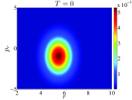
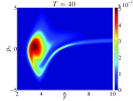
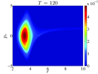
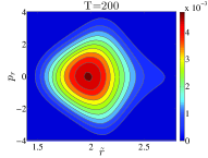
Figure 3: Snapshots of the distribution function from a typical near-critical calculation, with evolution proceeding left to right, top to bottom (note the reduction in the range of radial coordinate in the last frame). The displayed results are from family G8 (see Table 1) where $p_{c}$—which is loosely the average momentum of the initially imploding shell of particles—is the control parameter. As with all of the calculations discussed in the results section, the control parameter has been tuned to roughly machine precision. In the early stages of the evolution we observe phase space mixing and the ejection of some particles (the latter particularly visible as the “tail” in the second frame). At intermediate times the system approaches a static state which persists for a period that is long compared to the infall/dispersal timescale characterizing weak field dynamics. We note that this is a 3D calculation, with $f$ non-trivial in the $l$ direction: for visualization purposes we have integrated over $l$ to produce a quantity depending only on $r$ and $p_{r}$. Additionally, the first three frames are plotted using the computational coordinate, $r$, while for the purposes of direct comparison with Fig. 4, the fourth uses the rescaled coordinate, ${\tilde{r}}$, defined by (64). We emphasize that at criticality $f$ retains non-trivial dependence on $p_{r}$; that is, although the geometry is static, the particle behaviour is still dynamic.

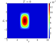
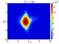
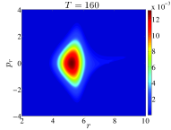
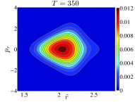
Figure 4: Snapshots of the distribution function for a near-critical calculation using family G10. Here the tuning parameter is the overall amplitude, $A$, of the initial particle distribution. As in the previous figure the sequence shows an approach to a static state, but it is evident that the form of the distribution function at criticality is significantly different in the two calculations. Due to the use of the rescaled radial coordinate, ${\tilde{r}}$, the fourth frames of the two figures can be meaningfully compared.

Here we use initial distribution functions, $f_{0}\equiv f(0,r,p_{r},l)$, that describe configurations of particles localized in $r$, $p_{r}$ and $l$, and that include various parameters which can be tuned to generate families of solutions that span the black hole threshold. Specifically, we set

$$f(0,r,p_{r},l^{2})=S(r,p_{r})F(l)\,,$$ (56)

where $S(r,p_{r})$ is given by either a gaussian function,

$$\mathcal{G}(r,p_{r};\,A,r_{c},p_{c})\equiv A\exp\left(-\frac{(r-r_{c})^{2}}{\Delta_{r}^{2}}-\frac{(p_{r}-p_{c})^{2}}{\Delta_{p}^{2}}\right)\,,$$ (57)

or the truncated bi-quadratic form

$$\mathcal{E}(r,p_{r};\,A,r_{c},p_{c})\equiv\left\{\begin{array}[]{l l }A\bar{r}(1-\bar{r})\bar{p}(1-\bar{p})&0<\bar{r}<1\,,\\ {}{}{}{}{}{}{}{}{}{}{}{}{}{}{}{}{}{}{}{}{}{}{}{}{}{}{}&0<\bar{p}<1\,,\\ $0$&\text{elsewhere,}\end{array}\right.$$ (58)

where $\bar{r}=(r-r_{c}+\Delta r)/2\Delta r$ and $\bar{p}=(p_{r}-p_{c}+\Delta p)/2\Delta p$. Note that the dependence of $\mathcal{G}$ and $\mathcal{E}$ on $r$ and $p_{r}$ is suppressed in the abbreviated notation used in Table 1. For the 3D calculations, we use two types of angular momentum distribution: the first is a gaussian,

$$F(l)=\exp\left(\frac{-(l-l_{0})^{2}}{\Delta l^{2}}\right)\,,$$ (59)

while the second is uniform in $l$ with cutoffs at some prescribed minimum and maximum values, $l_{\rm min}$ and $l_{\rm max}$, respectively,

$$F(l)=\Theta(l-l_{\rm min})\Theta(l_{\rm max}-l)\,.$$ (60)

It is important to point out that since the massless Einstein-Vlasov system is scale-free it has an additional symmetry relative to the massive case. Specifically, the equations of motion are invariant under the transformation

$$t\rightarrow kt\,,$$ (61)

$$r\rightarrow kr\,,$$ (62)

where $k$ is an arbitrary positive constant. In order to meaningfully compare results from different initial data choices we must therefore adopt unitless coordinates in our analysis. We do this by rescaling $t$ and $r$ by the total mass, $M^{\star}$, of the putatively static solution which arises at criticality for any of the families that we have considered (that is, $M^{\star}$ includes only the mass associated with that portion of the overall matter distribution which appears to be static at criticality). Moreover, it is more natural and convenient to use central proper time, $\tau$, rather than $t$ itself in the analysis. Thus, the results below are described using rescaled coordinates, $\tilde{\tau}$ and $\tilde{r}$, defined by

$$\tilde{\tau}=\frac{\tau}{M^{\star}}\,,$$ (63)

$$\tilde{r}=\frac{r}{M^{\star}}\,.$$ (64)

We note that under the scaling (61)–(62) the angular momentum transforms as

$$l\rightarrow kl\,.$$ (65)

The process we use to generate near-critical solutions is completely standard for this type of work. All of the family definitions described above and summarized in Table 1 contain multiple parameters that can be used to tune to the black hole threshold and, consistent with what has been found in many other previous studies of black hole critical phenomena, we find that which particular parameter is actually varied is essentially irrelevant for the results. Having chosen some specific parameter, $p$, to vary, any critical search begins by determining an initial bracketing interval, $[p_{l},p_{h}]$, in parameter space such that evolutions with $p_{l}$ and $p_{h}$ lead to dispersal and black hole formation, respectively. We then narrow the bracketing interval using a bisection search on $p$, predicating the update of $p_{l}$ or $p_{h}$ on whether or not a black hole forms. The search is continued until $(p_{h}-p_{l})/p_{h}\sim 10^{-15}$, so that $p^{\star}$ is computed to about machine precision (8-byte floating point arithmetic). The value of $p_{l}$ at the end of this process corresponds to what we dub the marginally sub-critical solution.

Quite generically, as we tune any family to a critical value $p^{\star}$, the phase space distribution function appears to settle down to a static solution which, as $p\to p^{\star}$, persists for a time that is long compared to the characteristic timescale for implosion and subsequent dispersal of the particles in the weakly-gravitating limit. Representative illustrations of this behaviour are shown for marginally sub-critical evolutions from two distinct initial data families in Fig. 3 (family G8 in Table 1) and Fig. 4 (family G10). Similarly, the spacetime geometry–encapsulated in the metric functions $a$ and $\alpha$—also becomes increasingly time-independent as criticality is approached. Fig. 5 displays the evolution of the $\ell_{2}$-norm of the time derivative of $a$ during marginally sub-critical evolution for family G1. We thus have strong evidence that the critical solutions that we are finding are static—characteristic of type I critical behaviour—and consistent with what has been observed previously for the case of the massive Einstein-Vlasov system.

Figure 5: Time evolution of $\|\partial_{t}a(t,r)\|_{2}$ from a marginally sub-critical calculation using family G1. The plot provides strong evidence that the geometry of the threshold solution is static, a characteristic feature of type I behaviour.

Figure 6: Lifetime scaling of near-critical configurations for families G8, G1, G10 and G4 (top to bottom and noting that G10 and G8 are 3D calculations while the others are 2D). Here the symbols plot estimates of the amount of time the state of the system is well approximated by the static critical solution—measured in units of the rescaled proper time defined by (63)—as a function of $\ln|p-p^{\star}|$. The lines are least squares fits to $\tau=-\sigma\ln|p-p^{\star}|$ where $\sigma$ is the reciprocal of the eigenvalue (Lyapunov exponent) corresponding to the presumed single growing mode of the critical solution. To the estimated level of accuracy in our calculations the measured values of $\sigma$ are the same for the three families. However, we cannot state with certainty that there is precise universality in this regard.

Figure 7: Radial metric function $a(\tilde{r})$ at criticality for families G8, G1, G10 and G4. The results plotted here, together with those displayed in Fig. 8, show that there is relatively little variation in the geometry of the static critical configuration as a function of the specifics of the initial data. The inset plots the deviation in $a$ for families G1, G10 and G4 relative to G8.

Figure 8: Lapse function $\alpha(\tilde{r})$ at criticality for families G8, G1, G10 and G4. The comments made in the caption of the previous figure apply here as well.

Further evidence for generic type I transitions in the model is provided by observations of lifetime scaling of the form (1) near criticality, which is expected if the critical solutions are one-mode unstable. Typical results from calculations using families G1, G4, G8 and G10 are shown in Fig. 6: the linearity of the lifetime of the static critical configuration as a function of $\ln|p-p^{\star}|$ is apparent. We have observed such scaling for all of the families that we have studied (in both the 2D and 3D cases) and Table 2 provides a summary of the measured values of the scaling exponent, $\sigma$.

We note that the specific form of the matter configuration at criticality exhibits significant dependence on the family of initial data that is used to generate the critical solution. This can be seen, for example, by comparing the last frames of Figs. 3 and 4. On the other hand, as illustrated in Fig. 7 and Fig. 8, the geometry of the critical state is relatively insensitive to the initial conditions.

The spacetime geometry can be characterized by the central red shift, $Z_{c}$ defined by (44), and the unitless compactness parameter, $\Gamma$, defined by

$$\Gamma={\rm max}_{r}\frac{2m}{r}\,.$$ (66)

For the families considered in this section the values of $\Gamma$ and $Z_{c}$ fall in the ranges

$$0.79\lesssim\Gamma\lesssim 0.81\,,$$ (67)

$$2.4\lesssim Z_{c}\lesssim 2.5\,.$$ (68)

As discussed in the next section, these ranges are relatively small in comparison to those found in our investigation of critical behaviour using nearly-static initial data.

What is striking about the results assembled in Table 2 is that there appears to be a small variation, at most, in the time scaling exponent associated with the critical solutions produced from our generic initial conditions. Specifically, the data is consistent with

$$\sigma=1.4\pm 0.1\,,$$ (69)

and we emphasize that this concordance arises despite the significant observed variation in the phase-space distribution of the particles among the various critical solutions.

Family	$l_{0}$	$\sigma$	Family	$l_{0}$	$\sigma$
G1	5	$1.32\pm 0.08$	G3	12	$1.36\pm 0.06$
G1	6	$1.35\pm 0.07$	G4	12	$1.37\pm 0.05$
G1	7	$1.36\pm 0.06$	G5	12	$1.44\pm 0.06$
G1	8	$1.33\pm 0.06$	G6	12	$1.43\pm 0.04$
G1	9	$1.33\pm 0.06$	G7	$6$ & $12$	$1.37\pm 0.07$
G1	10	$1.32\pm 0.06$	G8	10	$1.35\pm 0.05$
G1	11	$1.35\pm 0.05$	G9	10	$1.36\pm 0.05$
G1	12	$1.37\pm 0.05$	G10	-	$1.40\pm 0.05$
G2	-	$1.36\pm 0.07$

Table 2: Summary of measured lifetime scaling exponents for the massless Einstein-Vlasov model from experiments using the various initial data families enumerated in Table 1. In addition to the overall functional form of the initial distribution functions, a key parameter that varies among the sets of calculations is $l_{0}$, which is the angular momentum of any and all particles for families G1, G2–G6 (2D) and the center of the angular momentum distribution for families G8 and G9 (3D). ($l_{0}$ is the tuning parameter for G6, and family G7 is another special case where the initial data is comprised of a superposition of two shells of particles, each having a distinct angular momentum parameter. Since angular momentum is a conserved quantity there is no mixing of the two distributions during the evolution.) For simplicity of presentation we have not listed the other parameters defining the different initial configurations. Quoted uncertainties in the values of $\sigma$ are based on variations in the total mass of the system during the evolutions and comparison with results computed at lower resolution. Typical grid sizes used for the listed results are $n_{r}\times n_{p}=1024\times 1024$ (2D) or $n_{r}\times n_{p}\times n_{l}=256\times 128\times 64$ (3D). To the level of accuracy in our calculations we find consistency with a single value of the scaling exponent, $\sigma=1.4\pm 0.1$.

V.2 Near-static massless case

Our second approach to study critical solutions in the massless Einstein-Vlasov system starts with the construction of static initial data using the procedure described in Sec. III. We specialize the general form (41) to

$$\Phi(E,l)=C(1-E/E_{0})^{b}\Theta(E_{0}-E)\delta(l-l_{0})\,,$$ (70)

where $E_{0}$ is a given cutoff energy and $C$, $b$ and $l_{0}$ are additional adjustable parameters. Here we focus exclusively on the case of fixed angular momentum (2D calculations) since the results of the previous section suggest that the essential features of the critical solutions are not significantly dependent on whether or not $f$ has non-trivial dependence on $l$. In addition, from the scale free symmetry in the system (see (61) and (65)), we can conclude that varying the value of angular momentum is equivalent to rescaling the radial coordinate. Therefore, without loss of generality we can set $l$ to an arbitrary fixed value, eliminating one of the parameter-space dimensions in our surveys. Additionally, so that we can meaningfully compare results from different initial conditions, we again rescale the radial coordinate by the total mass of the system (64). Furthermore, by virtue of the transformation (43), the static profiles depend on $E_{0}$ only through the ratio $E_{0}/\alpha_{0}$ and, since it simplifies the numerical analysis, we actually use this ratio as one of the control parameters.

For specified values of the free parameters $C$, $b$ and $E_{0}/\alpha_{0}$, we integrate equations (29)–(32) outward until we reach a radial location, $r_{X}$, where the particle density $\Phi(E,l)$ vanishes. We then extend the solution for $a$ and $\alpha$ to the outer boundary of the computational domain by attaching a Schwarzschild geometry with the appropriate mass.

We note that not all choices of the three free parameters lead to distribution functions with compact support—that is, with $f(0,r,p_{r})\equiv 0$ for $r$ greater than some $r_{X}$—so that the configuration represents a single shell of particles. Indeed, by examining the expression for the particle energy in the massless case:

$$E(r,p_{r})=\alpha(r)\sqrt{(p_{r}/a)^{2}+(l/r)^{2}}\,,$$ (71)

we see that, for $p_{r}$ sufficiently small, $E(r,p_{r})$ can remain below the cutoff $E_{0}$ for large $r$. In practice this will yield solutions with multiple shells, where $\Phi$ vanishes at $r_{X}$, but then becomes non-zero on a infinite number of intervals in $r$ (in general these intervals can be disjoint or contiguous, as has previously been seen in Andréasson and Rein (2007)). Although it might be interesting to consider the critical dynamics of multiple-shell solutions, we do not do so here. We also note that for given values of $b$ and $E_{0}/\alpha_{0}$ we find solutions with a distinct shell (i.e. where $\Phi$ does vanish at some radius) only for a certain range of $C$, but that range can span several orders of magnitude.

Fig. 9 shows the distribution function for four sample static configurations constructed as described above, with the associated geometrical variables plotted in Fig. 10. Relative to the apparently static solutions generated by tuning generic initial data, the family-dependence of both the distribution function and metric variables here is much more pronounced.

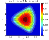
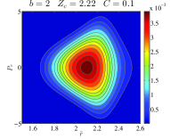
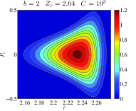
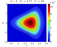
Figure 9: Sample static phase space configurations computed from the ansatz (70) using different choices of adjustable parameters. Note that although we use the rescaled radial coordinate ${\tilde{r}}$ in all of the plots, the ranges in ${\tilde{r}}$, $p_{r}$ and $f$ vary from frame to frame. Clearly, there is a strong dependence of $f$ on the chosen parameter values. As described in more detail in the text, for any given values of $b$ and $Z_{c}$ there is a finite range of $C$ for which we find static solutions where $f$ has compact support.

Figure 10: Plots of the radial metric function, $a(r)$, and differential particle number, $dN(r)/dr$, for the configurations shown in Fig. 9. The graphs of $dN(r)/dr$ highlight the fact that the critical solutions are shell-like, with a thicknesses and effective densities that are strongly dependent on the choice of parameters in (70).

One interesting way of characterizing the static solutions is to plot the compactness parameter, $\Gamma$, defined by (66), as a function of the central redshift, $Z_{c}$. We do this for a large number of configurations in Fig. 11 where, as described in more detail in the caption, each set of points results from a two-dimensional parameter space survey wherein both $E_{0}/\alpha_{0}$ and $C$ are varied. The fact that the solutions from each of these surveys tend to “collapse” to one-dimensional curves in $Z_{c}$–$\Gamma$ space is striking and we do not have any argument at this time for why this should be so.

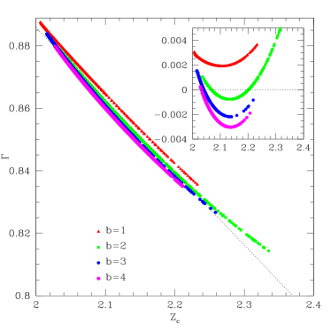
Figure 11: The value of $\Gamma={\rm max}_{r}(2m/r)$ versus central redshift, $Z_{c}$, for various static solutions. Each set of points comprises several thousand distinct solutions and comes from a two-dimensional parameter space survey, in which both $C$ and $E_{0}/\alpha_{0}$ are varied. Although for given $b$ and $E_{0}/\alpha_{0}$ we can only find acceptable static solutions in certain ranges of $C$, those ranges can span several orders of magnitude. However, for fixed $b$ the solutions tend to collapse to near-linear loci in $Z_{c}$–$\Gamma$ space, and the inset graph, which plots the deviation of the data from a linear least squares fit, is intended to emphasize this behaviour. More detailed examination of the data suggests that the configurations do not lie precisely along one-dimensional curves, but additional study would be required to determine whether this is really the case. The solutions apparently satisfy the Buchdahl inequality $\Gamma<8/9$ (also seen in the calculations reported in Andréasson and Rein (2007) for the massive case), as is expected from Andréasson‘s rigorous results Andréasson (2007). Moreover, there also seems to be a lower bound on the compactness, $\Gamma\sim 0.81$.

All of the static solutions that we have found satisfy Buchdahl’s inequality, $\Gamma<8/9$, originally derived in the context of fluid matter Buchdahl (1959), and the most compact configurations are quite close to that limit. Here it is crucial to note that Andréasson has proven rigorously that the Buchdahl inequality is satisfied by any static solution of the spherically symmetric Einstein-Vlasov system Andréasson (2007). Further, he has demonstrated that one can construct static shell-like configurations which, in the limit of infinitesimal thickness in $r$, can have $\Gamma$ arbitrarily close to $8/9$. Although not explicitly mentioned in Andréasson (2007), it is clear that his proof is valid for $m=0$. Given the nature of Andréasson‘s result, the observation that our solutions satisfy the bound clearly amounts to little more than additional evidence that our calculations are faithful to the model under study. However it is interesting that the highest values of $\Gamma$ seen in Fig. 11—and which plausibly are approaching $8/9$—are associated with very thin shell-like solutions. Additionally, for the configurations we have studied (not all of which are represented in Fig. 11) there is apparently also a lower bound on the compactness, $\Gamma\sim 0.81$. Finally, the ranges of $\Gamma$ and $Z_{c}$ spanned by the explicitly static solutions

$$0.80\lesssim\Gamma\lesssim 0.89\,,$$ (72)

$$2.0\lesssim Z_{c}\lesssim 2.4\,,$$ (73)

are larger than those seen for the tuned generic data, consistent with the comment above concerning the relatively large variations in the metric variables as well as the distribution function.

$b$	$Z_{c}$	$C$	$\delta f$	$\sigma$
$1$	$2.32$	$0.1$	$\delta f_{1}$	$1.45\pm 0.05$
$1$	$2.23$	$0.3$	$\delta f_{1}$	$1.45\pm 0.04$
$2$	$2.22$	$0.1$	$\delta f_{1}$	$1.43\pm 0.04$
$4$	$2.17$	$10$	$\delta f_{1}$	$1.43\pm 0.04$
$2$	$2.35$	$0.1$	$\delta f_{1}$	$1.40\pm 0.05$
$2$	$2.35$	$0.1$	$\delta f_{2}$	$1.40\pm 0.05$
$2$	$2.35$	$0.1$	$\delta f_{3}$	$1.40\pm 0.05$

Table 3: Measured lifetime scaling exponent for explicitly static solutions constructed from ansatz (70) with various choices of the adjustable parameters $b$, $E_{0}/\alpha_{0}$ and $C$ ($Z_{c}$ is effectively controlled by $E_{0}/\alpha_{0}$, but is determined a posteriori), and the different types of perturbations, $\delta f$, enumerated in (75)–(77). Proceeding from the assumption that the static solutions are characterized by a single unstable mode, we anticipate that the computed value of $\sigma$ associated with a specific configuration (i.e. for given $b$, $Z_{c}$ and $C$) should be independent of the form of $\delta f$, and this is precisely what we observe (compare rows 1 and 2, and 5, 6 and 7). However, we also see once again that there is little, if any, variation in the scaling exponent with respect to the underlying critical solution: the results in the table are consistent with $\sigma=1.43\pm 0.07$

Using our evolution code, we investigate the relation of the explicitly-static solutions to critical behaviour in the model as follows. For initial conditions we set

$$f(0,r,p_{r},l^{2})=f^{0}(r,p_{r},l^{2})+(A-1)\delta f(r,p_{r},l^{2})\,,$$ (74)

where $f^{0}$ is a static configuration, $\delta f(r,p_{r},l^{2})$ is some given perturbation function with at least roughly the same support as $f^{0}$, and $A$ is a tunable parameter which controls the amplitude of the perturbation. Clearly, $A=1$ results in initialization with the static solution itself. We have experimented with the following three choices for the perturbation function:

$$\delta f_{1}(r,p_{r},l^{2})=f^{0}(r,p_{r},l^{2})\,,$$ (75)

$$\delta f_{2}(r,p_{r},l^{2})=\sin\left(\frac{2\pi f^{0}(r,p_{r},l^{2})}{f_{\rm max}}\right)\,,$$ (76)

$$\delta f_{3}(r,p_{r},l^{2})=f^{0}(r,p_{r},l^{2})(f_{\rm max}-f^{0}(r,p_{r},l^{2}))p_{r}\,,$$ (77)

where $f_{\rm max}$ is the maximum of $f^{0}$ over the computational domain. We then perform standard tuning experiments in which we vary $A$ to isolate a threshold solution.

Interestingly, we find strong evidence that all of the static solutions based on (70) that we have found sit at the threshold of black hole formation, so that setting $A>1$ results in black hole formation while taking $A<1$ results in complete dispersal of the matter (or vice versa, dependent on the precise form of $\delta f$). As should be suspected then, and as is shown for four families in Fig. 12, the solutions generated by dynamically evolving the perturbed static configurations exhibit time scaling—this strongly suggests that the time-independent solutions are all one-mode unstable. Table 3 provides a summary of the time-scaling exponents we have measured for a set of experiments based on four distinct static solutions and the three different types of perturbation defined by (75)–(77).

Figure 12: Lifetime scaling computed from families of initial data based on the static configurations plotted in Figs. 9 and 10. The tuning parameter in this instance controls the amplitude of a perturbation that is added to the base solution (here we used the form $\delta f_{1}$ (75)) and, in all cases, the sign of the perturbation determines whether the evolution leads to dispersal or black hole formation. The results shown here provide evidence that the static configurations calculated from the ansatz (70) act as type I critical solutions. Additionally, we see that there is very little variation in the measured scaling exponents, $\sigma$, which are again determined via least squares fits to (1).

As was the case for the generic families, the measurements here indicate that although the static solutions display significant variation in both the distribution function and geometric variables, there is little variation in the scaling exponent. Here we find

$$\sigma=1.43\pm 0.07\,.$$ (78)

Recalling (69), and given the estimated uncertainty in our calculations, we can not exclude the possibility that $\sigma$ is truly universal for the massless-sector critical solutions which we have constructed. Particularly given the variation in the spacetime geometries involved, constancy of the eigenvalue of the unstable mode associated with criticality would be truly remarkable. However, even if $\sigma$ does span some finite range, the apparent tightness of that range is an aspect of critical behaviour in the massless system that begs understanding.

Finally, we note that the static critical solutions from the generic calculations are characterized by compactness, $\Gamma\sim 0.8$, which is at the low end of the range spanned by the explicitly static solutions. We do not yet know whether a more extensive parameter space survey of generic data could produce critical configurations with larger $\Gamma$, and it would be interesting to further investigate this issue.

V.3 Generic massive case

Following previous studies Rein et al. (1998); Olabarrieta and Choptuik (2001); Stevenson (2005), we have also examined the case where the particles have rest mass and find results that are in general agreement with the earlier work, including strong evidence for the existence of static solutions at the black hole threshold that exhibit lifetime scaling. However, we note that in both Olabarrieta and Choptuik (2001) and Stevenson (2005) the initial data configurations were kinetic energy dominated. For example, a typical calculation in Olabarrieta and Choptuik (2001) used unit particle mass and $f(0,r,p_{r},l)$ which was gaussian in the three coordinates with characteristic values $r\sim 3$, $p_{r}\sim 1$ and $l\sim 3$. From expression (35) for the particle energy we can thus infer that the initial data sets had kinetic energy about an order of magnitude larger than rest mass energy. Thus we expect that those previous results should be similar to what we see for massless particles. Indeed, taking into account the different time parameterization used ($t$ normalized to coincide with property time at infinity), the scaling exponents quoted in Olabarrieta and Choptuik (2001) are consistent with our results.

Table 4 lists the values of the time scaling exponent we have determined in the massive case for the various types of initial data defined in Table 1. We note that the initial data families that are used include ones that are very similar to those adopted in Olabarrieta and Choptuik (2001) and Stevenson (2005). We see that the time scaling exponents are in fact close to those measured in the massless calculations, although the spread in the values is noticeably larger here (as it was in Olabarrieta and Choptuik (2001) and Stevenson (2005)). This increased spread is almost certainly due to the particle mass—i.e. the evolutions are not completely kinetic energy dominated.

Paralleling what was done in Sec.V.2, as well as in Andréasson and Rein (2007), we can use perturbations of our explicitly static solutions in the massive sector to investigate critical behaviour. Here there is a larger function space of static configurations, especially since we can construct solutions with positive binding energy, $E_{b}$, defined by

$$E_{b}\equiv M_{0}-M\,,$$ (79)

where $M_{0}$ is the total rest mass and $M$ is the ADM mass. Moreover, we can build parameterized sequences of solutions that transition between positive and negative $E_{b}$, completely analogously to what can be done for perfect fluid models of general relativistic stars. As in the perfect fluid case, we anticipate that: 1) solutions with $E_{b}>0$ will be perturbatively stable, 2) there will be a change of stability at $E_{b}=0$, and 3) for at least some range of $E_{b}<0$, the static configurations will be one-mode unstable, and thus should constitute type I critical solutions. We have performed additional calculations that confirm these expectations. In particular, we were able to build a static solution with $E_{b}$ negative, but relatively close to 0, which did lie at the black hole threshold and which had an associated scaling exponent $\sigma=3.0\pm 0.1$. This value of $\sigma$ is clearly distinct from those listed in Table 4. Thus, in contrast to the massless case where we can not conclusively state anything about possible variations in $\sigma$ for type I critical solutions, we are confident that $\sigma$ is is not universal in the massive case. In fact, were we able to construct static configurations with $E_{b}\rightarrow 0^{-}$, we assume that we would find $\sigma\rightarrow\infty$. Again, these observations and conjectures are entirely consistent with previous studies of the Einstein-Vlasov system, as well as work with gravitationally compact stars modelled with perfect fluids or bosonic matter.

Family	$l_{0}$	$Z_{c}$	$\sigma$	Family	$l_{0}$	$Z_{c}$	$\sigma$
G1	5	2.47	$1.32\pm 0.14$	G1	12	2.28	$1.46\pm 0.07$
G1	6	2.39	$1.47\pm 0.13$	G2	-	2.39	$1.44\pm 0.09$
G1	7	2.31	$1.44\pm 0.08$	G3	9	2.29	$1.54\pm 0.07$
G1	8	2.37	$1.49\pm 0.08$	G4	9	2.43	$1.49\pm 0.08$
G1	9	2.41	$1.49\pm 0.08$	G8	10	2.24	$1.38\pm 0.14$
G1	10	2.34	$1.48\pm 0.07$	G9	10	2.41	$1.59\pm 0.15$
G1	11	2.23	$1.54\pm 0.07$

Table 4: Summary of measured lifetime scaling exponents for the massive Einstein-Vlasov model from experiments using the various initial data families enumerated in Table 1. The results quoted here derive from calculations that parallel those described in Table 2 for the massless system. In contrast to the massless case, the observed variation in $\sigma$ is significant.

VI Summary and Discussion

We have constructed a new numerical code to evolve the Einstein-Vlasov system in spherical symmetry using an algorithm where the distribution function $f(t,r,p_{r},l^{2})$ is directly integrated using finite volume methods. This approach eliminates the statistical uncertainty inherent in the particle-based techniques that have been used in previous studies. To reduce computational demands at a given discretization or, more importantly, to allow for higher resolution, we can also run the code in a 2D mode where $l^{2}$ is some fixed scalar constant so that $f$ depends on only $r$ and $p_{r}$.

We have used the code to perform extensive and detailed surveys of the critical behaviour in the model with a particular focus on the case where the particles are massless. We note that we are unaware of any previous dynamical numerical calculations pertaining to the massless sector.

Our results derive from two classes of initial configurations. In the first the initial states represents imploding shells of particles well removed from the origin, while the second involves perturbations of configurations that are precisely static by construction. Although time-independent solutions of the massive system have been constructed and analyzed previously, to our knowledge the static states we have found in the massless sector are the first of their kind. Within each class we have studied numerous specific forms for the initial data and, for the near-static calculations, the perturbations that are applied to generate the threshold behaviour. In all cases we find strong evidence for a Type I critical transition including: 1) a finite black hole mass at threshold and 2) lifetime scaling of the form (1). The observations are all consistent with the standard picture for Type I behaviour, namely a static critical solution with one unstable perturbative mode. Here we emphasize that—as is the case for any numerical study of critical behaviour—it is very difficult to preclude the existence of additional unstable modes. However, the degree to which the scaling laws are satisfied suggests that if such modes do exist they have growth rates significantly smaller than the dominant one.

For generic initial data with massless particles, we have found that there is a considerable variation in the morphology of $f$ among the different critical solutions we have computed and, to a lesser extent, in the details of the spacetime geometries encoded in $a(t,r)$ and $\alpha(t,r)$. Interestingly though, there is relatively little variation in the time scaling exponents that we have measured: all seem to be in the range $\sigma=1.4\pm 0.1$.

In the case of near-static initial conditions with $m=0$ the key results are quite similar. Again, there is a large variation in the functional form of the distribution function at threshold. In this instance this can be seen as a direct reflection of the freedom inherent in the ansatz (70) which involves the specification of two essentially arbitrary functions. Not surprisingly, there is thus a more noticeable range in the geometries at criticality relative to the generic calculations, as can be clearly seen, for example, through examination of quantities such as the compactness and central redshift. Once again, however, we observe only a small dispersion in the measured scaling exponents. Specifically, across all near-static families that we have examined we find $\sigma=1.43\pm 0.07$.

Thus, considering all of the calculations that we have performed, we have indications of at least a weak form of universality of the time-scaling exponent in the massless Einstein-Vlasov model. Here we note that as mentioned in the introduction, the calculations reported in Olabarrieta and Choptuik (2001) were also suggestive of a universal value of $\sigma$ and perhaps of the critical geometry. Those computations used a non-zero mass and, as also discussed previously, the work of Andréasson and Rein (2006, 2007) established that the spacetime structure at criticality could not be universal in the massive model. However, as noted in Sec. V.3 the initial data families used in Olabarrieta and Choptuik (2001) were kinetic energy dominated (effectively massless), and so there is no contradiction between what was seen there (and here) and Andréasson and Rein (2006, 2007).

In all of our calculations, and in accord with Andréasson’s proof of the Buchdahl inequality in the model Andréasson (2007), we observe that the gravitational compactness satisfies $\Gamma<8/9$ , with thin shell-like solutions coming closest to saturating the bound.

We also want to emphasize an additional feature of the massless model that is apparent from our calculations: the particle angular momentum does not have a significant impact on the features of the critical solution (apart from the obvious fact that the particles do have angular momentum in all of our computations). Heuristically, this can be at least partly ascribed to the scaling symmetry (61)–(62). The symmetry effectively reduces the number of free parameters—relative to a naive analysis—available for variation in the search for critical solutions. Specifically, given any distribution of the form $f(r,p_{r})\delta(l-l_{1})$, where $l_{1}$ is fixed, we can map to a distribution $f^{\prime}(r,p_{r})\delta(l-l_{2})$, with $l_{1}\neq\l_{2}$, which has an associated geometry that is diffeomorphic to the original.

Given that there is clearly no universality of the fundamental dynamical variables at threshold, the fact that the variation in $\sigma$ is, at most, small is a feature of the calculations for which we currently have no explanation. Additionally, as discussed in the introduction, the argument advanced in Martin-Garcia and Gundlach (2002) suggests that there should be no type I behaviour in the Einstein-Vlasov system for either the massless or massive models. At this time, we do not understand how—if at all—this argument can be reconciled with our current results and those from previous numerical studies.

A direct analysis of the perturbations of the critical solutions—especially the precisely static ones—would be very helpful at this point. Starting with the perfect-fluid work of Koike et al Koike et al. (1995), perturbation analyses of the critical configurations in many different models have been extremely effective in advancing our understanding of black-hole critical phenomena. In particular, relative to measurements made through direct solution of PDEs and tuning experiments, perturbative methods can provide highly accurate values for the eigenvalues of the unstable modes (or, equivalently, for the scaling exponents). However, in our case the task of explicitly constructing perturbations is significantly complicated by the fact that there is no one-to-one correspondence between the geometry and the phase-space distribution of the particles. So far we have been unable to formulate a well-defined approach to computation of the perturbations and will have to leave that for future work.

Finally, it would be interesting to extend this work to the Einstein-Boltzmann system, where the introduction of explicit interactions between particles would provide the means to investigate the connection between criticality in phase-space-based models and hydrodynamical systems. This in turn might lead to a more fundamental understanding of critical collapse in fluid models.