A Tabu Search Algorithm for the Multi-period Inspector Scheduling Problem

Abstract

This paper introduces a multi-period inspector scheduling problem (MPISP), which is a new variant of the multi-trip vehicle routing problem with time windows (VRPTW). In the MPISP, each inspector is scheduled to perform a route in a given multi-period planning horizon. At the end of each period, each inspector is not required to return to the depot but has to stay at one of the vertices for recuperation. If the remaining time of the current period is insufficient for an inspector to travel from his/her current vertex $A$ to a certain vertex $B$, he/she can choose either waiting at vertex $A$ until the start of the next period or traveling to a vertex $C$ that is closer to vertex $B$. Therefore, the shortest transit time between any vertex pair is affected by the length of the period and the departure time. We first describe an approach of computing the shortest transit time between any pair of vertices with an arbitrary departure time. To solve the MPISP, we then propose several local search operators adapted from classical operators for the VRPTW and integrate them into a tabu search framework. In addition, we present a constrained knapsack model that is able to produce an upper bound for the problem. Finally, we evaluate the effectiveness of our algorithm with extensive experiments based on a set of test instances. Our computational results indicate that our approach generates high-quality solutions.

1 Introduction

This paper studies a new manpower routing and scheduling problem faced by a company that procures products from over one thousand suppliers across Asia. The company places orders with a large number of suppliers and must inspect the goods at the factories of the suppliers before shipment. Therefore, the suppliers are required to make inspection requests with the company when the ordered goods are ready for delivery. An inspection request is characterized by the workload, the inspection site and the time window within which the inspection can be started. In turn, the company dispatches a team of professional quality inspectors to perform all on-site inspections. In order to facilitate coordination between inspectors and suppliers, the inspections could only be carried out during working hours (e.g., 8:00 am to 6:00 pm). Usually, a weekly schedule is created to assign inspectors to requests for the upcoming week. The company has a stable of in-house inspectors, each having a specified weekly workload limit, and the unfulfilled inspection requests are outsourced to external agencies with additional costs. After receiving their weekly inspection schedules, the inspectors depart from the regional office and will not report back until they have performed all their assigned inspections for the week. More specifically, they leave the regional office on Monday, visit a set of inspection sites and return to the regional office on Friday or some earlier workday. In each workday, an inspector generally travels to diffident locations, completes several inspections and finds overnight accommodation (i.e., hotel) in the vicinity of his/her last/next inspection site at or before the end of the office hours. The objective of the problem is to assign as many inspection workloads as possible to the stable of in-house inspectors while satisfying all the above-mentioned practical constraints.

We call this problem the multi-period inspector scheduling problem (MPISP), which can be viewed as a variant of the multi-trip vehicle routing problem with time windows (VPRTW) (Azi et al., 2010; Macedo et al., 2011). There are four main features that distinguish the MPISP from the multi-trip VRPTW. First, the scheduling subjects, e.g., vehicles or inspectors, are not required to return to the regional office every workday. Second, at the end of each workday, each scheduling subject must stay at one of the vertices for recuperation. Third, each vertex can be visited more than once. If the remaining time of the current period is insufficient for an inspector to travel from his/her current vertex $A$ to a certain vertex $B$, he/she can choose either waiting at vertex $A$ until the start of the next period or traveling to a vertex $C$ that is closer to vertex $B$. The vertex $C$ is called a waypoint, which only acts as the intermediate point in a route. Fourth, the objective is to maximize the total inspected workload rather than to minimize the number of inspectors used and/or the total distance traveled.

In this study, we propose a tabu search algorithm to solve the MPISP. This algorithm employs a tailored fitness function consisting of three lexicographically ordered components, a local improvement procedure with tabu moves, an ejection pool improvement process and a perturbation phase. The contributions of this study are fourfold. First, we introduce a new and practical multi-period manpower routing and scheduling problem that considers multiple working periods. Second, we provide an effective tabu search algorithm that uses a set of problem-specific neighborhood search operators. Third, we construct a constrained knapsack model that can produce an upper bound for the MPISP. Fourth, the comprehensive experimental results on a large number of test instances show the effectiveness of our approach.

The remainder of this paper is organized as follows. We first provide an overview of related research in Section 2. In Section 3, we then give a formal definition of the MPISP. In Section 4, we describe an approach of computing the shortest transit time for any pair of vertices with any departure time. Our proposed tabu search algorithm is detailed in Section 5 and the constrained knapsack model is presented in Section 6. Section 7 reports the experiments results and Section 8 concludes this study with some closing remarks.

2 Related work

The MPISP is one type of manpower scheduling problems. Scheduling staff members is a traditional research area; example problems include the nurse rostering problem (Cheang et al., 2003), the technician planning problem (Ernst et al., 2004) and the airline crew rostering problem (Kohl and Karisch, 2004). As for the manpower scheduling problems that involve creating routes for staff members, we refer the reader to Li et al. (2005); Tang et al. (2007); Zäpfel and Bögl (2008); Cai et al. (2013); Zhang et al. (2013).

Since each inspector has to perform inspections at different locations, the MPISP is essentially a variant of the vehicle routing problem (Toth and Vigo, 2002). One of the defining characteristics is its objective of maximizing the total inspected workload. Two previously studied problems with similar objective are the team orienteering problem with time windows (TOPTW) (Vansteenwegen et al., 2009, 2011; Labadie et al., 2012; Hu and Lim, 2014) and the vehicle routing problem with time windows and a limited number of vehicles ($m$-VRPTW) (Lau et al., 2003; Lim and Zhang, 2007). The $m$-VRPTW is an extension of the TOPTW with the consideration of vehicle capacity and customer demands. These two problems both aim to determine a set of routes that maximizes the total reward of the vertices visited during a single period with a distance or duration limit. The multi-period planning horizon of the MPISP is related to the periodic vehicle routing problem (PVRP) (Gaudioso and Paletta, 1992; Hemmelmayr et al., 2009) and the multiple trip vehicle routing problem (MTVRP) (Battarra et al., 2009). However, the MPISP is quite different from the PVRP and MTVRP. In the PVRP, each customer requires a certain number of visits within the planning horizon, and two types of decisions are involved in the planning, namely determining the visit days for each customer and the routing plan for each time period. The PVRP and MTVRP both require that each vehicle must return to the depot at the end of each period.

Another defining characteristic of the MPISP is the consideration of multiple working periods. Working hour regulations have recently received increasing attention from some researchers studying vehicle routing problems. Savelsbergh and Sol (1998) proposed a dynamic and general pickup and delivery problem in which lunch and night breaks must be taken into account. Xu et al. (2003) applied column generation based solution approaches to solve a pickup and delivery vehicle routing problem that involves a set of practical complications, such as heterogeneous vehicles, last-in-first-out loading and unloading operations, pickup and delivery time windows, and working hour restrictions by the United States Department of Transportation. Similarly, Goel (2009, 2010) and Kok et al. (2010) investigated combined vehicle routing and driver scheduling problems under the European Union regulations for drivers.

The MPISP problem can be viewed as a natural extension of the orienteering problem with hotel selection (OPHS) (Divsalar et al., 2013, 2014). In the OPHS, a scheduling subject can visit a set of vertices each with a score and find accommodation at a given set of hotels. The tour is divided into multiple trips, each with a limited duration and starting from and ending at one of the hotels. The objective of the OPHS is to determine a tour that maximizes the total collected score. The OPHS is a variant of the traveling salesperson problem with hotel selection (TSPHS) (Vansteenwegen et al., 2012; Castro et al., 2013), which aims to serve all vertices with the minimum number of connected trips and the minimum total travel distance. The common characteristic of the above three problems is the involvement of hotel selection.

Tang et al. (2007) and Zäpfel and Bögl (2008) introduced two manpower routing and scheduling problems that involve maximization of profits, multiple periods and working hour restrictions. However, their problems require that the trip in each period must start from and end at the depot. Most recently, Zhang et al. (2013) proposed an inspector scheduling problem which is very similar to our problem. Their problem differs from our problem in the following four assumptions: (1) each vertex can only be visited at most once; (2) if a vertex is visited by an inspector, its inspection request must be fulfilled by this inspector; (3) an inspector reaches a vertex and completes the corresponding inspection task in the same period; and (4) each vehicle stays at the last served vertex at the end of each period and begins the trip of the next period from that vertex. By ignoring these four assumptions, the MPISP is more difficult but practical.

3 Problem description

The MPISP is defined on a directed graph $G=(V,E)$, where $V=\{0,1,\ldots,n\}$ is the vertex set and $E=\{(i,j):i,j\in V,i\neq j\}$ is the edge set. Vertex 0 represents the depot location and $V_{C}=\{1,\ldots,n\}$ denotes the locations of $n$ suppliers. Each supplier $i$ is characterized by a location $i\in V_{C}$, a workload $d_{i}$, a required service time $s_{i}$ and a time window $[e_{i},l_{i}]$. For notational convenience, we assign $d_{0}=0$ and $s_{0}=0$ for the depot. Each edge $(i,j)\in E$ requires a non-negative traveling time $t_{i,j}$, where the matrix $[t_{i,j}]$ satisfies the triangle inequality.

We are given a set $K$ of $m$ homogeneous inspectors, each of which has a workload limit $Q$ and can only work within a set $P=\{1,\ldots,w\}$ of $w$ working periods (or called working time windows). For any period $p\in P$, $a_{p}$ and $b_{p}$ $(a_{p}<b_{p})$ are its starting and closing working times, respectively, and $b_{p}-a_{p}$ equals a positive constant $T$ that is not less than $s_{i}$ for any $i\in V$. An inspector can arrive at vertex $i\in V_{C}$ prior to $e_{i}$ and wait at no cost until the service of supplier $i$ becomes possible. All inspectors must leave the depot after $e_{0}$ $(e_{0}=a_{1}=0)$ and return to the depot before $l_{0}$ $(l_{0}=b_{w})$, where $[e_{0},l_{0}]$ is called depot time window. At the end of each period, each inspector is not required to return to the depot but has to stop traveling and stay at one of vertices. Moreover, service cannot be interrupted, i.e., if the service of some supplier cannot be completed before the end of a period, it must be restarted in the later periods. Each vertex can be visited more than once while each supplier can be served by at most one inspector, so some supplier locations can be used as waypoints. The objective of the MPISP is to construct $m$ inspector routes to complete as many workloads as possible while respecting depot time window, workload limit, supplier time windows and inspector working time windows. We provide a mixed integer programming model for the MPISP in Appendix A.

In reality, $a_{p}$ should be larger than $b_{p-1}$, and the duration between $a_{p}$ and $b_{p-1}$ is the downtime for rest and recuperation. Without loss of generality, we can assume that the length of the downtime is extremely small by setting $b_{p-1}=a_{p}$ and imposing a break at time $b_{p-1}$. As illustrated in Figure 1, we can easily transform the non-zero downtime cases to zero downtime ones. In Figure 1(a), $T=20$ and the time windows of suppliers 1, 2, and 3 are $[5,90]$, $[10,50]$ and $[85,95]$, respectively. After transformation, their time windows become [5, 50], [10, 30] and [45, 55] (see Figure 1(b)).

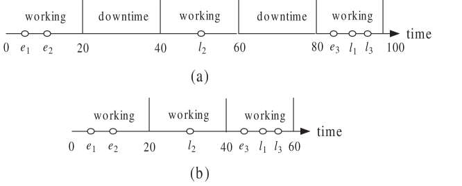
Figure 1: (a) The original case. (b) The case after transformation.

To further describe the MPISP, we convert the graph $G=(V,E)$ into a directed (not complete) graph $G^{\prime}=(V^{\prime},E^{\prime})$ by the following two steps: (1) split each vertex $i\in V_{C}$ into two vertices $i+$ and $i-$, and create an edge $(i+,i-)$, where vertex $i+$ represents the arrival of vertex $i$ and vertex $i-$ represents the completion of supplier $i$’s service; (2) create edges $(0,i+)$, $(i+,0)$, $(i-,0)$, $(i+,j+)$ and $(i-,j+)$, where $i,j\in V_{C}$ and $i\neq j$; and (3) set $t_{i+,i-}=s_{i}$, $t_{0,i+}=t_{0,i}$, $t_{i+,0}=t_{i-,0}=t_{i,0}$ and $t_{i+,j+}=t_{i-,j+}=t_{i,j}$. An example to illustrate this conversion is shown in Figure 2, where Figure 2(b) is the resultant graph derived from Figure 2(a).

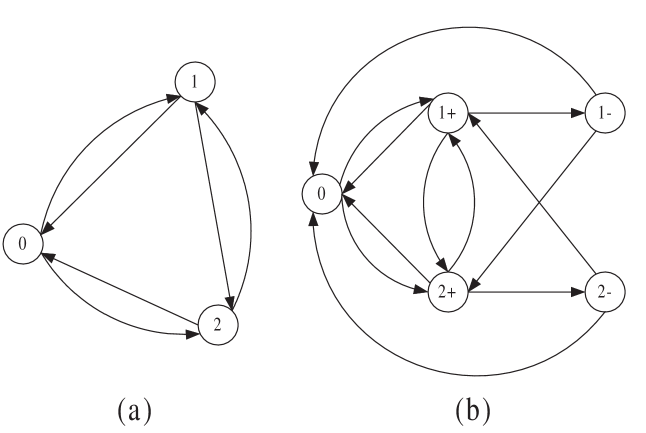
Figure 2: (a) $G=(V,E)$. (b) $G^{\prime}=(V^{\prime},E^{\prime})$.

We can denote a feasible solution of the MPISP by $S$, consisting of $m$ routes, namely $S=\{r_{1},r_{2},\ldots,r_{m}\}$. A route $r_{k}$ $(1\leq k\leq m)$ is divided into $w$ sub-routes by periods and therefore can be expressed as $r_{k}=(r_{k}^{1},r_{k}^{2},\ldots,r_{k}^{w})$, where $r_{k}^{p}$ $(1\leq p\leq w)$ denotes the trip in period $p$. If an inspector returns to the depot before period $w$, he/she will stay at the depot for the remaining periods. The sub-route $r_{k}^{p}$ is a sequence of vertices, where its starting and ending vertices are denoted by $v_{s}(r_{k}^{p})$ and $v_{e}(r_{k}^{p})$, respectively. If an inspector $k$ stays at the depot during the whole period $p$, we set $r_{k}^{p}=(0)$ and $v_{s}(r_{k}^{p})=v_{e}(r_{k}^{p})=0$. According to the definition of our problem, an inspector must stay at vertex $v_{e}(r_{k}^{p})$ for rest and will start the next trip from this vertex in period $p+1$, i.e, $v_{e}(r_{k}^{p})=v_{s}(r_{k}^{p+1})$ for all $1\leq p\leq w-1$. Obviously, the starting vertex of period $1$ and the ending vertex of period $w$ for each route must be vertex $0$. Figure 3 gives a feasible solution to an MPISP instance involving 10 suppliers, 4 inspectors and 3 periods.

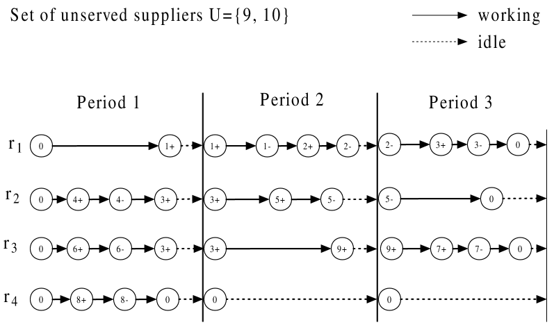
Figure 3: An example feasible solution to an MPISP instance.

In Figure 3, the solid and dash lines denote the working (i.e., traveling or providing service) and idle statuses of the inspectors, respectively. The set $U=\{9,10\}$ indicates that suppliers 9 and 10 are not served by any inspector. The route $r_{1}=(r_{1}^{1},r_{1}^{2},r_{1}^{3})$ comprises three trips, i.e., $r_{1}^{1}=(0,1+)$, $r_{1}^{2}=(1+,1-,2+,2-)$ and $r_{1}^{3}=(2-,3+,3-,0)$. This route shows that inspector 1 arrives at vertex 1, but does not have sufficient time to complete the service for supplier 1 in the first period. Thus, he/she has to wait until the start of the second period and then provides service to supplier 1. Subsequently, inspector 1 travels to vertex 2, completes the service of supplier 2 and stays at vertex 2 for recuperation. In the third period, inspector 1 travels from vertex 2 to vertex 3, provides service for supplier 3, and finally returns to the depot. Since each supplier $i$ can be served by at most one inspector, edge $(i+,i-)$ can be included in at most one route. In route $r_{2}$, after completing the service of supplier 4, inspector 2 travels to vertex 5 via a waypoint, namely vertex 3. Note that any waypoint must be the ending vertex of a certain period (and also be the starting vertex of the following period) due to the rule of triangle inequality. As shown in route $r_{3}$, an inspector may use two or more waypoints between two consecutively served suppliers. In this route, inspector 3 visits but does not serve supplier 9, i.e., vertex 9 only acts as a waypoint. As no route traverses edge $(9+,9-)$, supplier 9 is not served by any inspector in this solution. The route $r_{4}$ illustrates that an inspector may be idle during some periods; its three trips are represented by $r_{4}^{1}=(0,8+,8-,0)$, $r_{4}^{2}=(0)$ and $r_{4}^{3}=(0)$.

4 Shortest transit time

In a complete graph that satisfies the triangle inequality, the shortest path from vertex $i$ to vertex $j$ must be edge $(i,j)$. When working periods are imposed on the inspectors, edge $(i,j)$ may be unusable in some situations and therefore the shortest transit time may be greater than $t_{i,j}$. The simplest such situation can be encountered when $t_{i,j}>T$. To move from vertex $i$ to vertex $j$, an inspector has to use some waypoints and the transit time may cross several periods. We illustrate this situation in Figure 4, where an inspector has completed the service of supplier $i$ and departs from vertex $i$ at the beginning of a certain period.

Figure 4: (a) The vertex locations. (b) The route associated with the shortest transit time from vertex $i$ to vertex $j$, where vertices $i_{1}$ and $i_{2}$ are waypoints.

Unlike the classical VRP models, in the MPISP the shortest transit times from vertex $i$ to other vertices are affected by the departure time (denoted by $dt_{i}$) of the inspector. Therefore, we define $\hat{t}_{i,j}(dt_{i})$ as the shortest transit time from vertex $i$ to vertex $j$ with departure time $dt_{i}$. If $dt_{i}$ is the opening time of a certain period, i.e., $dt_{i}=a_{p}$ for some $p\in P$, $\hat{t}_{i,j}(dt_{i})$ can be simplified to $\hat{t}_{i,j}$. Further, we define $ceil(dt_{i})$ as the closing time of the period within which $dt_{i}$ lies, i.e., if $a_{p}<dt_{i}\leq b_{p}$, then $ceil(dt_{i})=b_{p}$. If $ceil(dt_{i})-dt_{i}\geq t_{i,j}$, an inspector can travel across edge $(i,j)$ within the current period and thus $\hat{t}_{i,j}(dt_{i})=t_{i,j}$. Otherwise, the inspector has to either wait at vertex $i$ until the start of the next period or travel to some waypoint $u$. We illustrate these situations in Figure 5, where an inspector may travel from vertex $i$ to vertex $j$ via some waypoint.

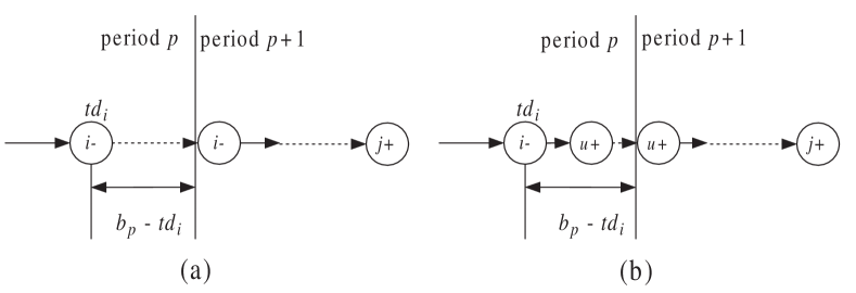
Figure 5: (a) Wait at vertex $i$. (b) Travel to a waypoint $u$.

As previously mentioned, a waypoint $u$ can only be positioned as the last or the first vertex in the trip of some period. More precisely, if an inspector travels to a waypoint $u$, he must stay at $u$ for downtime (see Figure 5(b)). Taking $N(dt_{i})=\{u\in V|t_{i,u}\leq ceil(dt_{i})-dt_{i}\}$ to be the set of all vertices that can act as waypoints for vertex $i$, the value of $\hat{t}_{i,j}(dt_{i})$ can be calculated by:

$$\hat{t}_{i,j}(dt_{i})=\left\{\begin{array}[]{ll}t_{i,j},&\textrm{if $ceil(dt_{i})-dt_{i}\geq t_{i,j}$};\\ ceil(dt_{i})-{dt}_{i}+\min_{u\in N(dt_{i})\cup\{i\}}\{\hat{t}_{u,j}\},&\textrm{otherwise.}\end{array}\right.$$ (3)

The above expression shows that computing any $\hat{t}_{i,j}(dt_{i})$ requires $O(n)$ time given the values of all $\hat{t}_{i,j}$, which can be calculated prior to applying any algorithm to the problem. If the last waypoint between vertex $i$ and vertex $j$ is vertex $u$, the corresponding shortest transit time, denoted by $\hat{t}^{u}_{i,j}$, can be obtained by:

$$\hat{t}^{u}_{i,j}=\left\{\begin{array}[]{ll}\hat{t}_{i,u}+t_{u,j},&\textrm{if $ceil(\hat{t}_{i,u})-\hat{t}_{i,u}\geq t_{u,j}$};\\ ceil(\hat{t}_{i,u})+t_{u,j},&\textrm{if $ceil(\hat{t}_{i,u})-\hat{t}_{i,u}<t_{u,j}\leq T$; }\\ +\infty,&\textrm{otherwise.}\end{array}\right.$$ (7)

Obviously, we have:

$$\hat{t}_{i,j}=\min_{u\in V}\{\hat{t}^{u}_{i,j}\}$$

To compute all $\hat{t}_{i,j}$, we can apply an algorithm modified from the Dijkstra’s algorithm (Ahuja et al., 1993), one of the most well-known label-setting algorithms for the classical shortest path problem. This modified Dijkstra’s algorithm employs expression (7) as the extension function and has a time complexity of $O(n^{2})$. Since we need to compute the shortest transit time between each vertex pair, the total time complexity for all $\hat{t}_{i,j}$ is bounded by $O(n^{3})$.

We can accelerate the computation of $\hat{t}_{i,j}(dt_{i})$ by the following procedure. We first remove from the graph all edges whose lengths are greater than $T$ and then sort all neighbors $u$ of vertex $i$ in ascending order of $t_{i,u}$, generating a vertex sequence $(i_{0},i_{1},\ldots,i_{h})$. Note that we have $i_{0}=i$ since $t_{i,i}=0$. For $0\leq k\leq h$, let $\hat{t}_{i,j}^{(k)}=\min_{0\leq k^{\prime}\leq k}\{\hat{t}_{i_{k^{\prime}},j}\}$ be the shortest transit time from one of the first $k+1$ vertices in the sequence to vertex $j$. The values of all $\hat{t}_{i,j}^{(k)}$ can be computed by Algorithm 1 in time complexity of $O(n^{3})$. Figure 6 pictorially shows the process of computing all $\hat{t}_{i,j}^{(k)}$. According to expression (3), $\hat{t}_{i,j}(dt_{i})$ = $ceil(dt_{i})-{dt}_{i}+\min_{u\in N(dt_{i})\cup\{i\}}\{\hat{t}_{u,j}\}$ if $ceil(dt_{i})-dt_{i}<t_{i,j}$. To achieve this $\hat{t}_{i,j}(dt_{i})$, we identify the largest $k$ satisfying $ceil(dt_{i})-dt_{i}\geq t_{i,i_{k}}$ using binary search on $t_{i,i_{0}},t_{i,i_{1}},\ldots,t_{i,i_{h}}$, and retrieve the value of $\hat{t}_{i,j}^{(k)}$, which is equal to $\min_{u\in N(dt_{i})\cup\{i\}}\{\hat{t}_{u,j}\}$. The above procedure shows that the time complexity of computing $\hat{t}_{i,j}(dt_{i})$ can be reduced to $O(logn)$ given that all $\hat{t}_{i,j}^{(k)}$ are available.

Figure 6: The process of computing all $\hat{t}^{(k)}_{i,j}$.

Algorithm 1 The algorithm for preprocessing all $\hat{t}_{i,j}^{(k)}$.

1:  INPUTS: all $\hat{t}_{i,j}$;

2:  for $i=0$ to $n$ do

3:     Sort all neighbors $u$ of vertex $i$ in ascending order of $t_{i,u}$ to generate a vertex sequence $(i=i_{0},i_{1},\ldots,i_{h})$;

4:     for $j=0$ to $n$ do

5:        $\hat{t}_{i,j}^{(0)}=\hat{t}_{i,j}$;

6:        for $k=1$ to $h$ do

7:           $\hat{t}_{i,j}^{(k)}=\min\{\hat{t}_{i,j}^{(k-1)},\hat{t}_{i_{k},j}\}$;

8:        end for

9:     end for

10:  end for

The computation of all $\hat{t}_{i,j}$ and $\hat{t}_{i,j}^{(k)}$ can be done in a preprocessing stage, which requires a time complexity of $O(n^{3})$. The approach described in the following section needs to frequently compute $\hat{t}_{i,j}(dt_{i})$. Thus, this preprocessing stage is particularly useful to save the overall computation time.

5 Tabu search algorithm

Tabu search algorithm has been successfully applied to a wide variety of routing and scheduling problems, such as the classical VRP (Gendreau et al., 1994; Toth and Vigo, 2003), the VRPTW (Chiang and Russell, 1997; Gordeau et al., 2001), the three-dimensional loading capacitated VRP (Zhu et al., 2012), the job-shop scheduling problem (Barnes and Chambers, 1995) and the nurse rostering problem (Burke et al., 2003). Basically, tabu search algorithm starts from an initial solution and iteratively proceeds from the incumbent solution to its best allowable neighbor. The neighborhood of a solution is a set of solutions that can be reached from that solution by a certain operation. Each type of operation corresponds to a neighborhood and the procedure of identifying the best allowable neighbor in the neighborhood is called an operator. The transition from the incumbent solution to one of its neighbors is called a move.

Our tabu search algorithm employs several operations adapted from classical operations for the VRPTW, namely 2-opt, Or-opt, 2-opt^∗, Relocate and Exchange (Bräysy and Gendreau, 2005), and an ejection pool (Lim and Zhang, 2007; Nagata and Bräysy, 2009). The most noteworthy characteristic that distinguishes these adapted operations from their classical counterparts is the procedure of checking the feasibility of the modified solution. For example, after performing an operation on a VRPTW solution, we can check the feasibility of the resultant solution in $O(1)$ time (it is assumed that for each vertex the latest arrival time that does not lead to the violation of the time windows of all successive vertices has been calculated in a preprocessing step). However, for a modified MPISP solution, we may require up to $O(nlogn)$ time to check its feasibility due to the re-computation of the shortest transit times associated with the affected vertices, which will be elaborated in Section 5.4.1.

The pseudocode of our tabu search algorithm is presented in Algorithm 2, which is an iterative approach that follows a four-phase framework: initialization, local search with tabu moves, ejection pool algorithm and perturbation. At the beginning of the algorithm, we generate an initial solution $S_{0}$ using the function best_init (see Section 5.3) and then initialize both the best solution $S_{best}$ and the current solution $S$ by $S_{0}$. In each iteration, we first invoke the local search procedure with tabu moves (function local_search, see Section 5.4) and set $S^{\prime}$ to be the best solution found by this procedure. Subsequently, we try to improve on $S^{\prime}$ by an ejection pool algorithm (function EPA, see Section 5.5) and then update $S_{best}$ if possible. Finally, the search process is diversified by perturbing the best solution found in this iteration. The above process is repeated until the perturbation procedure (function perturb, see Section 5.6) is consecutively performed maxPerturbation times without improving on $S_{best}$.

Algorithm 2 Framework of the tabu search algorithm.

1:  $S_{0}$ $\leftarrow$ best_init();

2:  $S_{best}$ $\leftarrow$ $S_{0}$ and $S$ $\leftarrow$ $S_{0}$;

3:  $i$ $\leftarrow$ $0$;

4:  while $i\leq$ maxPerturbation do

5:     $S^{\prime}$ $\leftarrow$ the best solution found by local_search($S$);

6:     $S^{\prime}$ $\leftarrow$ $EPA(S^{\prime})$

7:     if $S^{\prime}$ is better than $S_{best}$ then

8:        $S_{best}$ $\leftarrow$ $S^{\prime}$ and $i$ $\leftarrow$ 0;

9:     else

10:        $i$ $\leftarrow$ $i+1$;

11:     end if

12:     $S$ $\leftarrow$ perturb ($S^{\prime}$);

13:  end while

14:  return  $S_{best}$.

5.1 Solution representation

In Section 3, we have used the sequences of visited vertices to represent the problem solution (see Figure 3). However, in our tabu search algorithm, we represent the route of each inspector by a sequence of served suppliers. For example, Figure 7 shows a solution that is exactly the same as the one in Figure 3. The routes $r_{1},r_{2},r_{3}$ and $r_{4}$ include the served suppliers and the ejection pool $U$ contains the leftover suppliers. All waypoints are not displayed in this solution representation and there may exist waypoints and/or breaks between two consecutively served suppliers.

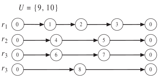
Figure 7: An example of the solution representation used in our tabu search algorithm.

5.2 Fitness function

The tabu search algorithm ranks solutions using a fitness function. It is natural to define the fitness value of a solution $S$ as the total completed workload, denoted by $P(S)$. However, many distinct solutions have the same value of $P(S)$. To further differentiate solutions, we incorporate into the fitness function another two measures denoted by $D(S)$ and $F(S)$, respectively, which is inspired by Lim and Zhang (2007). As a result, the fitness function consists of three lexicographically ordered components, namely $P(S)$, $D(S)$ and $F(S)$.

The second component $D(S)$ employs a function $mv(u,S)$ that estimates the difficulty of inserting supplier $u\in U$ into the routes of solution $S$. Denoting any route in $S$ by $r=(v_{0},v_{1},\ldots,v_{|r|},v_{|r|+1})$, where $|r|$ is the number of served suppliers in route $r$ and $v_{0}=v_{|r|+1}=0$, the definition of $mv(u,S)$ is given by:

$$mv(u,S)=\min_{r\in S}mv(u,r)$$

where

$$mv(u,r)=\max\Big{\{}\eta\times mv_{l}(u,r),~{}~{}mv_{t}(u,r)\Big{\}}$$ (8)

$$mv_{l}(u,r)=\left\{\begin{array}[]{ll}0,&\textrm{if $wl(r)+d_{u}\leq Q$};\\ (l_{0}-e_{0})\times\frac{(wl(r)+d_{u}-Q)}{wl(r)+d_{u}},&\textrm{otherwise.}\end{array}\right.$$ (11)

$$wl(r)=\sum_{v\in r}d_{v}$$

$$mv_{t}(u,r)=\min_{0\leq i\leq|r|}c(u,v_{i},r)$$

$$c(u,v_{i},r)=\max\Big{\{}{ea}^{\prime}_{u}-{l}_{u},0\Big{\}}+\max\Big{\{}e_{u}-{la}^{\prime}_{u},0\Big{\}}+\max\Big{\{}{ea}^{\prime}_{v_{i+1}}-{la}_{v_{i+1}},0\Big{\}}$$ (12)

The cost of inserting supplier $u$ into route $r$, denoted by $mv(u,r)$, is computed based on the extent of violating the workload limit and the time-window constraint. The amount of workload is translated into time unit by expression (11), where $wl(r)$ is the cumulative workload in route $r$. If the inspector has enough capability to serve supplier $u$, namely $wl(r)+d_{u}\leq Q$, then no workload penalty is incurred. Otherwise, the penalty, denoted by ${mv}_{l}(u,r)$, equals the length of the depot time window multiplied by the workload violation percentage.

The penalty for time-window violation, denoted by $mv_{t}(u,r)$, considers all possible insertions. For each $v_{i}\in r$, we can easily find its earliest arrival time ${ea}_{v_{i}}$ when $(0,v_{1},\ldots,v_{i})$ is feasible, and its latest arrival time ${la}_{v_{i}}$ that does not affect the feasibility of $(v_{i+1},v_{i+2},\ldots,v_{|r|},0)$. Inserting $u$ into $r$ at the position immediately after $v_{i}$ creates a new route $r^{\prime}$, which may be infeasible. Under the condition that $(0,v_{1},\ldots,v_{i})$ is feasible, we can find the earliest arrival times at $u$ and $v_{i+1}$ in $r^{\prime}$, denoted by ${ea}^{\prime}_{u}$ and ${ea}^{\prime}_{v_{i+1}}$, respectively. The partial route $(0,v_{1},\ldots,v_{i},u,v_{i+1})$ may be infeasible, i.e., ${ea}^{\prime}_{u}>l_{u}$ and/or ${ea}^{\prime}_{v_{i+1}}>l_{v_{i+1}}$. Furthermore, we can also find the latest arrival time at $u$, denoted by ${la}^{\prime}_{u}$, that makes $(v_{i+1},v_{i+2},\ldots,v_{|r|},0)$ feasible. The penalty for time-window violation incurred by inserting $u$ between $v_{i}$ and $v_{i+1}$ is calculated by summing up the violations of $l_{u}$, $e_{u}$ and ${la}_{v_{i+1}}$ (see expression (12)). As shown in expression (8), the cost of inserting $u$ into $r$ takes into account both ${mv}_{l}(u,r)$ and ${mv}_{t}(u,r)$ whose relative weights are controlled by a parameter $\eta$. After sorting the $mv(u,S)$ values of all unserved suppliers in ascending order, we can obtain a sequence $({mv}_{1},\ldots,{mv}_{|U|})$, where $|U|$ is the cardinality of $U$. The value of $D(S)$ is calculated by $\sum_{i=1}^{|U|}{mv}_{i}/i$. We believe that the solution $S$ with smaller $D(S)$ has more chance to be improved by including the unserved suppliers.

The third component $F(S)$ is the summation of the maximal free times of all routes in $S$. The maximal free time of route $r$ is defined as $mft(r)=\max_{0\leq i\leq|r|+1}\{{la}_{i}-{ea}_{i}\}$ and accordingly $F(S)=\sum_{r\in S}mft(r)$.

5.3 Initialization

We obtain an initial feasible solution for the tabu search algorithm using Algorithm 3. This algorithm first generates $N_{init}$ feasible solutions using the function init (see Algorithm 4) and then chooses the best one as the initial solution. In each iteration of init, we begin with computing the shortest transit time ${st}^{r}_{i}$ from the tail of each route $r$ to each unserved supplier $v_{i}$. If $v_{i}$ cannot be feasibly appended at the tail of $r$, we set ${st}_{i}^{r}=+\infty$. Next, we calculate the ratio of ${st}^{r}_{i}$ to $d_{i}$ and set $\rho_{i}$ to be the minimal ratio of $v_{i}$ over all routes (see Algorithm 4, line 11). If the value of $\rho_{i}$ is positive infinity, i.e., $v_{i}$ cannot be appended at the tail of any route, we remove $v_{i}$ from $U$. Finally, we sort all suppliers in $U$ by increasing value of $\rho_{i}$ and relocate the $k$-th supplier $v_{s}$ from $U$ to the tail of the route $r$ who has $\rho_{s}={st}^{r}_{s}/d_{s}$. The value of $k$ is a random number generated by $k=\lfloor random(0,1)^{\alpha_{1}}\times|U|\rfloor$, where the controlling parameter $\alpha_{1}>1$. This process is repeated until $U$ becomes empty.

Algorithm 3 Function best_init.

1:  Initialize $S_{0}=\emptyset$;

2:  while $i\leq N_{init}$ do

3:     $S=init()$;

4:     if $S$ is better than $S_{0}$ then

5:        $S_{0}$ $\leftarrow$ $S$;

6:     end if

7:     $i=i+1$;

8:  end while

9:  return  $S_{0}$.

Algorithm 4 Function init.

1:  INPUT: the set $U$ of unserved suppliers and $m$ empty routes;

2:  while $U$ is not empty do

3:     for  each $v_{i}$ in $U$ do

4:        for $r=1,\ldots,m$ do

5:           if $v_{i}$ can be feasibly appended to the tail of $r$ then

6:              ${st}_{i}^{r}$ $\leftarrow$ the shortest transit time from the last supplier of $r$ to $v_{i}$;

7:           else

8:              ${st}^{r}_{i}$ $\leftarrow$ $+\infty$;

9:           end if

10:        end for

11:        $\rho_{i}=\min_{r=1}^{m}\{{st}_{i}^{r}/d_{i}\}$;

12:        if $\rho_{i}=+\infty$ then

13:           Remove $v_{i}$ from $U$;

14:        end if

15:     end for

16:     Sort all suppliers in $U$ by increasing value of $\rho_{i}$;

17:     $v_{s}$ $\leftarrow$ the $k$-th supplier in the sorted supplier list, where $k=\lfloor random(0,1)^{\alpha_{1}}\times|U|\rfloor$ and $\alpha_{1}>1$;

18:     Append $v_{s}$ at the tail of $r$ with ${st}_{s}^{r}/d_{s}=\rho_{s}$;

19:     Remove $v_{s}$ from $U$;

20:  end while

5.4 Local search with tabu moves

The pseudocode of the local search procedure with tabu moves is provided in Algorithm 5. The following context of this subsection presents all main components of this procedure, including neighborhood structure, tabu list, aspiration and termination criteria.

Algorithm 5 The local search procedure with tabu moves (local_search).

1:  INPUT: the initial solution $S$;

2:  The current best solution $S^{\prime}$ $\leftarrow$ $S$ and Iter $\leftarrow$ 0;

3:  while $Iter\leq maxLocalIter$ do

4:     Apply the 2-opt, Or-opt, 2-opt^∗, relocate and exchange operators on $S$ ;

5:     $S$ $\leftarrow$ the best allowable solution found by the above operators;

6:     if $S$ is better than $S^{\prime}$ then

7:        $S^{\prime}\leftarrow S$ and $Iter$ $\leftarrow$ $0$;

8:     else

9:        $Iter$ $\leftarrow$ $Iter+1$;

10:     end if

11:     Update the tabu list;

12:  end while

13:  return  $S^{\prime}$.

5.4.1 Neighborhood structure

The neighborhood structure is one of the most important components that determine the size of the search space and the quality of the final solution. Our tabu search algorithm employs five neighborhood operations adapted from classical operations for the VRPTW (Bräysy and Gendreau, 2005), namely 2-opt, Or-opt, 2-opt^∗, Relocate and Exchange. We treat the ejection pool as a dummy route that includes all unserved suppliers. Compared with their classical counterparts, these adapted operations require more computational efforts to check the feasibility of the resultant solution, and to update the earliest and latest arrival times at the affected suppliers.

Figure 8 illustrates the 2-opt and Or-opt operations. Assume that we are given the earliest and latest arrival times (${ea}_{i}$ and ${la}_{i}$) at each supplier $i$ in route $r$. The earliest departure time (${ed}_{i}$) of each supplier can be easily derived by:

$${ed}_{i}=\left\{\begin{array}[]{ll}{ea}_{i}+s_{i},&\textrm{if $ceil(ea_{i})-ea_{i}\geq s_{i}$};\\ ceil({ea}_{i})+{s}_{i},&\textrm{otherwise.}\end{array}\right.$$ (15)

Figure 8: (a) The original route $r$. (b) The resultant route $r^{\prime}$ after a 2-opt operation. (c) The resultant route $r^{\prime}$ after an Or-opt operation.

The 2-opt operation replaces edges ($i,i+1$) and $(j,j+1)$ with edges $(i,j)$ and $(i+1,j+1)$, and then reverses the directions of all edges between $i+1$ and $j$. The resultant route $r^{\prime}$ shown in Figure 8(b) must be feasible if its subroute $(j,j-1,\ldots,i+1,j+1,\ldots,0)$ is feasible. To check the feasibility of $r^{\prime}$, we need to re-calculate the earliest arrival time (${ea}^{\prime}_{k}$) at each supplier $k$ in subroute $(j,j-1,\ldots,i+1,j+1)$. If ${ea}^{\prime}_{k}$ is less than $e_{k}$ or within $[e_{k},l_{k}]$ for each supplier, this subroute must be feasible. If ${ea}^{\prime}_{j+1}$ in $r^{\prime}$ is less than or equal to ${la}_{j+1}$ in $r$, subroute $(j+1,\ldots,0)$ must be feasible. All $ea^{\prime}_{k}$ can be obtained in $O(n_{s}logn)$ time using the procedure described in Section 4, where $n_{s}$ is the number of suppliers in subroute $(j,j-1,\ldots,i+1,j+1)$. Therefore, it requires $O(n_{s}logn)$ time to check the feasibility of route $r^{\prime}$. By contrast, when dealing with the VRPTW, a 2-opt operation only requires $O(n_{s})$ time to accomplish the feasibility check. In addition, updating the values of ${ea}^{\prime}_{i}$ and ${la}^{\prime}_{i}$ for all suppliers in $r^{\prime}$ requires $O(|r|logn)$ time and computing the fitness of the resultant solution requires $O(|r||U|logn)$ time.

The Or-opt operation replaces three edges ($i-1$), ($i+1,i+2$) and ($j,j+1$) with edges ($i-1,i+2$), ($j,i$) and ($i+1,j+1$); the resultant route is illustrated in Figure 8(c). After an Or-opt operation, we can also derive the time complexity for checking the feasibility of the resultant route, updating the earliest and latest arrival times at each supplier, and computing the fitness of the resultant solution in a manner similar to that used for the 2-opt operation.

Figure 9 illustrates the 2-opt^∗ operation which exchanges the latter subroutes of $r_{1}$ and $r_{2}$ by replacing edges ($i,i+1$) and ($j,j+1$) with edges ($i,j+1$) and ($j,i+1$). The feasibility of the resultant routes can be checked by simply comparing ${ea}^{\prime}_{j+1}$ (resp. ${ea}^{\prime}_{i+1}$) with ${la}_{j+1}$ (resp. ${la}_{i+1}$) in $O(logn)$ time. After this operation, we need $O((|r_{1}|+|r_{2}|)logn)$ time to update ${ea}^{\prime}_{i}$ and ${la}^{\prime}_{i}$ in $r^{\prime}_{1}$ and $r^{\prime}_{2}$ and $O((|r_{1}|+|r_{2}|)|U|logn)$ time to update the fitness of the resultant solution.

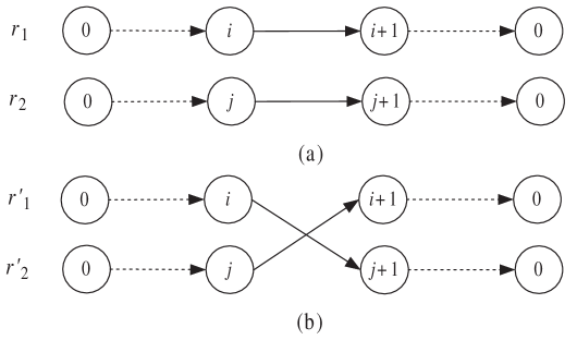
Figure 9: (a) The original routes $r_{1}$ and $r_{2}$. (b) The resultant routes $r^{\prime}_{1}$ and $r^{\prime}_{2}$ after a 2-opt^∗ operation.

The relocate operation can either relocate supplier $j$ in route $r_{1}$ to another position in the same route or to route $r_{2}$, which is illustrated in Figure 10. In the former case, the feasibility of the resultant route shown in Figure 10(b) can be checked by calculating ${ea}^{\prime}_{i}$ for all suppliers in subroute $(j,i+1,\ldots,j-1,j+1)$. In the latter case, we only need to check the feasibility of $r^{\prime}_{2}$ shown in Figure 10(c), which can be done in $O(logn)$ time. The relocation operation can also relocate a supplier in the ejection pool to a certain route or vice versa.

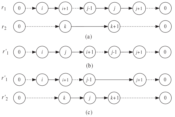
Figure 10: (a) The original routes $r_{1}$ and $r_{2}$. (b) The resultant routes $r^{\prime}_{1}$ after relocating supplier $j$ between suppliers $i$ and $i+1$. (c) The resultant routes $r^{\prime}_{1}$ and $r^{\prime}_{2}$ after relocating supplier $j$ between suppliers $k$ and $k+1$.

The exchange operation exchanges positions of two suppliers. Figure 11(b) shows the resultant route after exchanging the positions of two suppliers in the same route. The feasibility of this route can be checked by calculating ${ea}^{\prime}_{i}$ for all suppliers in subroute $(j,i+1,\ldots,j-1,i,j+1)$. The resultant routes created by exchanging two suppliers from two different routes are shown in Figure 11(c). The feasibility check can be done in $O(logn)$ time. This operation can also exchange a supplier in some route with a supplier in the ejection pool.

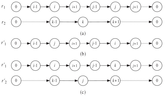
Figure 11: (a) The original routes $r_{1}$ and $r_{2}$. (b) The resultant routes $r^{\prime}_{1}$ after exchanging suppliers $i$ and $j$. (c) The resultants routes $r^{\prime}_{1}$ and $r^{\prime}_{2}$ after exchanging suppliers $j$ and $k$.

5.4.2 Tabu list, aspiration and termination

Tabu search algorithm employs one or more tabu lists to prevent the search process from being trapped in local optima. In our implementation, the tabu list stores edges that have been created within the previous $\xi$ iterations. A move is considered as tabu if it attempts to remove the edges in the tabu list. The tabu restriction can be overridden if the aspiration criterion is satisfied. Specifically, we allow the tabu moves to be performed if the solutions they result in are better than the current best solution $S^{\prime}$. The solutions that are created by non-tabu moves or by aspiration are called allowable neighbors. All allowable moves are stored in a candidate list and sorted according to the fitness values of their resultant solutions. The best candidate is performed to generate the next incumbent solution. We terminate the local search procedure when maxLocalIter consecutive iterations are unable to improve on $S^{\prime}$.

5.5 Ejection pool

Ejection pool has been previously used in the algorithms for reducing the number of routes for some routing problems (see for example Lim and Zhang (2007); Nagata and Bräysy (2009); Cheang et al. (2012)). Our ejection pool algorithm (EPA) is presented in Algorithm 6. The initial solution $S^{\prime}$ of this algorithm is the best solution found by function local_search. Since $S^{\prime}$ is a local optimum, no supplier in the ejection pool can be feasibly inserted into $S^{\prime}$. The EPA generates a candidate solution based on $S^{\prime}$ for each of the unserved suppliers by an insertion-ejection procedure. If the best candidate solution is superior to $S^{\prime}$, then $S^{\prime}$ is updated.

Algorithm 6 The ejection pool algorithm (EPA).

1:  INPUT: the initial feasible solution $S^{\prime}$;

2:  for each $u\in U$ do

3:     Evaluate all insertion positions using the function $c(i,u,j)$;

4:     $S_{u}$ $\leftarrow$ the resultant solution after inserting $u$ into $S^{\prime}$ at the best position;

5:     Eject suppliers one by one using the function $c(i)$ until $S_{u}$ becomes feasible;

6:     Improve $S_{u}$ by function local_search with $\xi=0$;

7:  end for

8:  if the best candidate solution $S_{u}$ is better than $S^{\prime}$ then

9:     $S^{\prime}$ $\leftarrow$ $S_{u}$;

10:  end if

11:  return  $S^{\prime}$.

For each $u\in U$, we evaluate its insertion positions using function $c(i,u,j)$, namely the cost of inserting $u$ between two consecutively served suppliers $i$ and $j$, which is defined as:

$$c(i,u,j)=\beta_{1}\times d_{u}-\beta_{2}\times\bigg{(}\max\Big{\{}0,ea^{\prime}_{u}-l_{u}\Big{\}}+\max\Big{\{}0,ea^{\prime}_{j}-l_{j}\Big{\}}\bigg{)},$$

where $\beta_{1}$ and $\beta_{2}$ are controlling parameters, and $ea^{\prime}_{u}$ and $ea^{\prime}_{j}$ are the earliest arrival times at suppliers $u$ and $j$ after inserting $u$ between $i$ and $j$. The position with the smallest value of $c(i,u,j)$ is selected for insertion.

The target route $r_{t}$ becomes infeasible after the insertion. Thus, some of its suppliers (except the newly inserted one) need to be ejected one by one until its feasibility is restored. The supplier $i$ to be ejected is determined based on the value of $c(i)$, which is defined as:

$$c(i)=\beta_{3}\times d_{i}+\beta_{4}\times\max\Big{\{}wl(r^{\prime}_{t})-Q,0\Big{\}}+\beta_{5}\times violation_{tw}(r^{\prime}_{t}),$$

where $\beta_{3}$, $\beta_{4}$ and $\beta_{5}$ are controlling parameters, $r^{\prime}_{t}$ is the resultant route after removing $i$ from $r_{t}$, and $violation_{tw}(r^{\prime}_{t})$ is the total time-window violation of all suppliers in route $r^{\prime}_{t}$, defined as:

$$violation_{tw}(r^{\prime}_{t})=\sum_{j\in r^{\prime}_{t}}\max\Big{\{}0,ea^{\prime}_{j}-l_{j}\Big{\}}.$$

The supplier $i$ with minimal $c(i)$ is ejected from the route $r_{t}$.

After performing the insertion-ejection procedure on each $u\in U$, we obtain $|U|$ candidate solutions, which are further improved by local_search without tabu moves, namely $\xi=0$. The solution $S^{\prime}$ is updated by the best candidate solution if possible.

5.6 Perturbation

The perturbation procedure is a diversification scheme that helps the search process escape from local optima. Our perturbation procedure (function perturb) randomly removes some suppliers from the solution $S^{\prime}$ following the rule that the suppliers with smaller workloads have more chances to be removed. Given a solution $S^{\prime}$, we sort the served suppliers in non-decreasing order of workloads, generating a supplier list $(v_{1},v_{2},\ldots,v_{n^{\prime}})$. The probability of removing the $k$-th supplier is determined by:

$$p_{min}+(p_{max}-p_{min})\times\frac{k}{n^{\prime}},$$ (16)

where $p_{min}$ and $p_{max}$ are controlling parameters satisfying $0\leq p_{min}\leq p_{max}\leq 1$. It implies that the supplier with larger workload has smaller probability to be kicked out.

The tabu search algorithm performs at least maxPerturbation iterations (see line 4 – 13, Algorithm 2). We store the best solution $S^{\prime}$ found within each iteration in a solution list. The solutions with equal values of $P(S)$, $D(S)$ and $F(S)$ are regarded as the same. The number of times that the current solution $S^{\prime}$ appears in the solution list is represented by $N_{rep}$. When $N_{rep}$ grows large, we expect that the perturbed solution deviates far from the current solution $S^{\prime}$. To this end, we replace $p_{min}$ and $p_{max}$ in expression (16) by:

$$p_{min}\leftarrow p_{min}+p_{\Delta}\times\min\{N_{rep},N_{max}\},$$

$$p_{max}\leftarrow p_{max}+p_{\Delta}\times\min\{N_{rep},N_{max}\},$$

where $p_{\Delta}$ is a controlling parameter, and the parameter $N_{max}$ is used to set an upper bound for the probability. The introduction of $N_{max}$ can help avoid the overly large probability, which would cause the process to degenerate into an ineffective multi-start method.

6 Upper bound

The solutions generated by our tabu search algorithm are lower bounds to the MPISP. In this section, we construct a constrained knapsack model to produce an upper bound for the MPISP; this model is motivated by Lau et al. (2003).

The time windows of all suppliers can be adjusted based on the following straightforward observations. For a supplier $i$, if the opening time of its time window lies within period $p$, i.e., $a_{p}\leq e_{i}\leq b_{p}$, and it is impossible to complete its service during that period, i.e., $b_{p}-e_{i}<s_{i}$, then the real earliest service starting time for supplier $i$ should be the opening time $a_{p+1}$ of the next period. Consequently, in this situation $e_{i}$ can be updated by $e_{i}=a_{p+1}$. Analogously, if $a_{p}\leq l_{i}\leq b_{p}$ and $b_{p}-l_{i}<s_{i}$, we can update $l_{i}$ by $l_{i}=b_{p}-s_{i}$. Let $\lambda_{i}=ceil({l}_{i}+s_{i})+\hat{t}_{i,0}$ denote the time of returning to the depot immediately after severing supplier $i$ with the service starting time $l_{i}$. We construct a supplier set $V_{G}=\{g_{1},g_{2},\ldots,g_{m}\}\subseteq V_{C}$ that contains $m$ distinct suppliers satisfying $\lambda_{i}\geq\lambda_{j}$ for all $i\in V_{G}$ and $j\in V_{C}\backslash V_{G}$.

Obviously, if $e_{i}>l_{i}$, supplier $i$ cannot be served by any inspector and vertex $i$ can only be used as a waypoint. We define $f_{1}(i)=0$ if $e_{i}>l_{i}$ and $f_{1}(i)=1$ otherwise. Suppose $e_{i}$ and $l_{i}$ lie within periods $p_{1}$ and $p_{2}$, respectively. We define $f_{2}(i,p)=1$ if $p_{1}\leq p\leq p_{2}$ and $f_{2}(i,p)=0$ otherwise, where $f_{2}(i,p)=1$ indicates that supplier $i$ could probably be served during period $p$. Furthermore, we use $f_{3}(i,j)=1$ to indicate that it is possible for an inspector to serve both suppliers $i$ and $j$ when supplier time windows, workload capacity and working periods are not considered. Thus, the definition of $f_{3}(i,j)$ is:

$$f_{3}(i,j)=\left\{\begin{array}[]{ll}1,&\textrm{if $e_{i}+s_{i}+t_{i,j}\leq l_{j}\textrm{ or }e_{j}+s_{j}+t_{j,i}\leq l_{i}$};\\ 0,&\textrm{otherwise.}\end{array}\right.$$

We denote by $r_{i}^{p}$ the time required to directly travel from supplier $i$ to its nearest neighbor who could probably be served by the same inspector during period $p$. Define set $V_{i}^{p}=\{j\in V|j\neq i,f_{2}(j,p)=1,f_{3}(i,j)=1\}$. We set $r_{i}^{p}=+\infty$ if $V_{i}^{p}$ is empty, and otherwise $r_{i}^{p}=\min_{j\in V_{i}}\{t_{i,j}\}$. Let $x_{i,k,p}$ be a binary decision variable that equals 1 if supplier $i$ is served by inspector $k$ during period $p$, and 0 otherwise. The optimal solution value of the following integer programming model gives an upper bound to the MPISP:

$$\max\sum_{i\in V_{C}}\sum_{k\in K}\sum_{p\in P}d_{i}x_{i,k,p}$$ (17)

s.t. $$\sum_{k\in K}\sum_{p\in P}x_{i,k,p}\leq f_{1}(i),~{}\forall~{}i\in V_{C}$$ (18)

$$\sum_{k\in K}x_{i,k,p}\leq f_{2}(i,p),~{}\forall~{}i\in V_{C},~{}p\in P$$ (19)

$$\sum_{p\in P}(x_{i,k,p}+x_{j,k,p})\leq 1+f_{3}(i,j),~{}\forall i,j\in V_{C},i\neq j,k\in K$$ (20)

$$\sum_{i\in V_{C}}\sum_{p\in P}d_{i}x_{i,k,p}\leq Q,~{}\forall~{}k\in K$$ (21)

$$\sum_{i\in V_{C}}\sum_{p\in P}\Big{(}s_{i}+\min\{r_{i}^{p},r_{i}^{p+1},\ldots,r_{i}^{w}\}\Big{)}x_{i,k,p}+r_{0}^{1}\leq\lambda_{g_{k}},~{}\forall~{}k\in K$$ (22)

$$\sum_{i\in V_{C}}x_{i,k,p}(s_{i}+r_{i}^{p})-\max_{i\in V_{C}}r_{i}^{p}\leq T,~{}\forall~{}k\in K,~{}p\in P$$ (23)

$$x_{i,k,p}\in\{0,1\},~{}\forall~{}i\in V_{C},~{}k\in K,~{}p\in P$$ (24)

The objective (17) is to maximize the total completed workload. Constraints (18) state that each supplier must be assigned to at most one inspector and be served in at most one period. Constraints (19) guarantee that if supplier $i$ cannot be served by any inspector during period $p$, all relative variables must be set to zero. Constraints (20) ensure that if $f_{3}(i,j)=0$, suppliers $i$ and $j$ cannot be served by the same inspector. As the inspector workload capacity cannot be exceeded, Constraints (21) apply. When supplier $i$ is served by some inspector, the time it consumes must be at least the sum of $s_{i}$ and the traveling time to its nearest neighbor. Any feasible solution to the MPISP must have $m$ routes, each of which has an earliest time of returning to the depot. It is easy to observe that the $k$-th largest return time must be less than or equal to the $k$-th largest $\lambda_{g_{k}}$. Obviously, the sum of $s_{i}+\min\{r_{i}^{p},r_{i}^{p+1},\ldots,r_{i}^{w}\}$ associated with all suppliers covered by a route should be less than or equal to the length of that route, which is capped by $\lambda_{g_{k}}$. Therefore, Constraints (22) hold. After completing the service of supplier $i$, the inspector may stay at vertex $i$ until the start of the next period. The difference between the total $s_{i}+r_{i}^{p}$ of all suppliers served in each period and the largest $r_{i}^{p}$ must be less than or equal to the period length, which is ensured by Constraints (23).

Any feasible solution to the MPISP must be also feasible to the constrained knapsack model (17) – (24). The knapsack problem and many of its variants have been well-studied and can be efficiently handled by several commercial mathematical programming solvers.

7 Computational experiments

Our tabu search (TS) algorithm was coded in C++ and compiled using the gcc 4.6.1 compiler, and was tested on a Dell server with an Intel Xeon E5430 2.66GHz CPU, 8 GB RAM and running Linux-CentOS-5.0 64-bit operating system. The algorithm was configured with determined parameter settings: $\eta=1.0$, $N_{init}=100$, $\alpha_{1}=5$, maxPerturbation = 4, maxLocalIter = 200, $\xi=100$, $\beta_{1}=0.6$, $\beta_{2}=\beta_{3}=\beta_{4}=0.4$, $\beta_{5}=0.2$, $p_{min}=0.05$, $p_{max}=0.30$, $p_{\Delta}=0.1$ and $N_{max}=5$. The MPISP reduces to the traditional TOPTW when $w=1$ and $Q=+\infty$. In our experiments, we first applied the TS algorithm to the TOPTW instances and compared the results with the recent results reported in Vansteenwegen et al. (2009); Lin and Yu (2012); Labadie et al. (2012); Hu and Lim (2014). Next, we conducted experiments on the MPISP instances generated from the Solomon’s VRPTW instances (Solomon, 1987). Since our TS algorithm is not deterministic, we solved each instance ten times. Finally, we achieved an upper bound for each MPISP instance by solving the model (17) – (24) using ILOG CPLEX 12.1 with default settings. Computation times reported are in CPU seconds on this server. All instances and detailed results can be found online at: http://www.computational-logistics.org/orlib/mpisp/.

7.1 Test instances

We considered the TOPTW instances used in Vansteenwegen et al. (2009); Hu and Lim (2014), which can be accessed at http://www.mech.kuleuven.be/en/cib/op. Hu and Lim (2014) classified these instances into two categories, namely “INST-M” and “OPT”; the instances in category INST-M have unknown optimal solution values while the optimal solution values of the instances in category OPT are given.

The TOPTW instances in category INST-M were constructed by Montemanni and Gambardella (2009) based on the OPTW instances by considering the number of vehicles taken from set {1, 2, 3, 4}. These OPTW instances were designed by Righini and Salani (2009) using 56 Solomon’s VRPTW instances (Solomon, 1987) and 20 Cordeau’s multi-depot VRP (MDVRP) instances (Cordeau et al., 1997). The Solomon’s VRPTW instances, each containing 100 customers, are divided into six groups, namely C1 (c101 – c109), C2 (c201 – c208), R1 (r101 – r112), R2 (r201 – r211), RC1 (rc101 – rc108) and RC2 (rc201 – rc208). The numbers of customers in the MDVRP instances (pr01 – pr20) range from 48 to 288. The TOPTW instances were obtained from the VRPTW or MDVRP instances by the following two steps: (1) set the profit collected at each customer to be the demand of this customer, and (2) remove the vehicle capacity restriction. The instances in category OPT are the same as the instances in category INST-M except for the number of vehicles available. Vansteenwegen et al. (2009) designed the instances in category OPT by setting the number of vehicles in each aforementioned TOPTW instance except for pr11 – pr20 to the number of vehicles appearing in the solution of the corresponding VRPTW instance. This implies that with such number of vehicles, all customers can be visited and the optimal objective value must be equal to the total profits of all customers. Therefore, we have 76 $\times$ 4 = 304 instances in category INST-M and 66 instances in category OPT, for a total of 370 TOPTW instances.

We generated 12 MPISP instances from each Solomon’s VRPTW instance by taking the values of $w$ and $m$ from {1, 3, 5} and {7, 9, 11, 13}, respectively, for a total of 72 instance groups (each instance group is identified by the name of Solomon’s instance group, $w$ and $m$) and 672 instances. The workload of each supplier is set to be the demand of the corresponding vertex. The duration of each period is set to $T=(l_{0}-e_{0})/w$ and the workload limit of each inspector is set to 200. The total profits in the MPISP instances related to the Solomon’s instance groups C1, C2, R1, R2, RC1 and RC2 are 1810, 1810, 1458, 1458, 1724 and 1724, respectively.

7.2 Results for the TOPTW instances

To evaluate the performance of our algorithm based on the TOPTW instances, we considered the following four state-of-the-art existing algorithms in our comparisons:

• ILS: the iterated local search algorithm by Vansteenwegen et al. (2009).

• SSA: the slow version of the simulated annealing algorithm by Lin and Yu (2012).

• GVNS: the LP-based granular variable neighborhood search algorithm by Labadie et al. (2012).

• I3CH: the iterative three-component heuristic (I3CH) by Hu and Lim (2014).

Lin and Yu (2012) proposed two versions of simulated annealing algorithm for the TOPTW, namely a fast version and a slow one. Compared with the fast version, the slow simulated annealing algorithm (SSA) is able to find better solutions at the expense of more computation time. As we are more concerned with solution quality, we used the SSA rather than the fast version in the comparisons. For each TOPTW instance, the ILS, SSA and I3CH were executed only once while the GVNS was performed five times. Although these algorithms were coded in different programming languages and executed on different computational environments (see Table 1), we believe that there is no dramatic difference between the speeds of these algorithms and it is acceptable to directly compare their computation times.

Table 1: Programming languages and experimental environments.

Algorithm	Language	Experimental environment
ILS	N/A	Intel Core 2 2.5 GHz CPU, 3.45 GB RAM
SSA	C	Intel Core 2 2.5 GHz CPU
GVNS	Embarcadero Delphi 2010	Intel Pentium (R) IV 3 GHz CPU
I3CH	Java	Intel Xeon E5430 CPU clocked at 2.66 GHz, 8 GB RAM
TS	C++	Intel Xeon E5430 CPU clocked at 2.66 GHz, 8 GB RAM

Table 2 summarizes the results of the TS, ILS, SSA, GVNS and I3CH for the TOPTW instances. We first identified the best solution value (BSV) obtained by these five algorithms and then computed the ratio of the best solution value produced by each algorithm to the BSV. The columns “Ratio (%)” and “Time (s)” show the average ratios and average computation times of all instance groups. Since Labadie et al. (2012) did not report the best solution value in their article, we filled the corresponding cells with “N/A” and ignored these cells when calculating the overall average ratio. Beside the name of each algorithm, we give the number of times it was run for each instance. The overall average values of “Ratio (%)” and “Time (s)” are presented in the last row and the best ratios in each row are marked in bold. All of the detailed solutions can be found in Appendix B.

Table 2: The summarized results for the TOPTW instances.

Instance Group	ILS (1 run)			SSA (1 run)			GVNS (5 runs)			I3CH (1 run)			TS (10 runs)
	Ratio (%)	Time (s)		Ratio (%)	Time (s)		Ratio (%)	Time (s)		Ratio (%)	Time (s)		Ratio (%)	Time (s)
$m$ =1
C1	0.9889	0.3		1.0000	21.1		0.9944	166.5		1.0000	25.2		1.0000	7.2
C2	0.9772	1.7		0.9987	37.5		0.9945	192.4		0.9960	84.4		1.0000	68.2
R1	0.9815	0.2		0.9995	23.3		0.9834	29.4		0.9950	28.6		1.0000	4.0
R2	0.9731	1.7		0.9891	45.8		0.9776	33.8		0.9916	176.2		0.9970	110.7
RC1	0.9708	0.2		1.0000	22.2		0.9812	9.8		0.9834	25.5		0.9958	2.9
RC2	0.9699	1.6		0.9947	50.3		0.9789	16.0		0.9774	119.3		0.9974	157.2
pr01 – pr20	0.9318	1.9		0.9801	137.3		0.9850	18.3		0.9768	119.6		0.9938	536.8
$m$ =2
C1	0.9906	1.1		1.0000	26.4		0.9953	139.5		1.0000	87.0		1.0000	21.8
C2	0.9746	3.5		0.9882	53.7		0.9975	33.8		0.9933	401.2		1.0000	63.8
R1	0.9777	0.9		0.9991	36.6		0.9895	60.3		0.9955	63.0		0.9970	14.1
R2	0.9702	2.3		0.9917	91.4		0.9909	14.7		0.9955	526.8		0.9992	91.5
RC1	0.9771	0.7		1.0000	40.5		0.9940	20.3		0.9928	58.9		0.9952	11.6
RC2	0.9593	2.2		0.9883	80.1		0.9839	12.8		0.9945	439.7		0.9995	243.2
pr01 – pr20	0.9311	5.0		0.9699	187.8		0.9915	60.8		0.9825	275.8		0.9935	1,809.5
$m$ = 3
C1	0.9745	1.5		0.9967	35.3		0.9955	165.0		0.9989	190.2		1.0000	31.1
C2	0.9807	2.2		0.9876	59.7		0.9993	7.7		1.0000	12.3		1.0000	6.8
R1	0.9832	1.7		0.9972	56.1		0.9889	73.9		0.9990	118.3		0.9983	16.6
R2	0.9970	1.4		0.9992	41.9		0.9989	7.0		0.9999	90.8		1.0000	14.8
RC1	0.9695	1.1		0.9946	42.8		0.9918	33.7		0.9982	101.0		0.9944	14.3
RC2	0.9856	1.7		0.9973	59.0		0.9968	7.4		0.9996	164.1		0.9998	52.1
pr01 – pr20	0.9213	9.5		0.9695	224.4		0.9933	118.3		0.9928	460.5		0.9895	1,680.5
$m$ = 4
C1	0.9689	2.6		0.9945	49.5		0.9897	133.2		0.9990	261.8		1.0000	38.6
C2	1.0000	1.0		1.0000	41.8		1.0000	0.6		1.0000	0.1		1.0000	6.5
R1	0.9670	2.6		0.9929	58.4		0.9880	84.7		0.9986	184.3		0.9956	21.0
R2	1.0000	0.9		1.0000	39.7		1.0000	0.3		1.0000	0.2		1.0000	7.7
RC1	0.9693	2.0		0.9974	68.1		0.9916	36.9		0.9988	152.4		0.9975	17.7
RC2	1.0000	1.2		1.0000	40.2		1.0000	0.9		1.0000	0.2		1.0000	15.5
pr01 – pr20	0.9249	13.9		0.9719	269.8		0.9872	180.0		0.9988	647.6		0.9940	1,542.4
$m$ = opt
C1	0.9859	3.0		0.9896	77.7		N/A	7.8		1.0000	47.6		1.0000	61.8
C2	1.0000	1.1		1.0000	41.9		N/A	0.5		1.0000	0.6		1.0000	113.3
R1	0.9807	3.0		0.9958	104.7		N/A	39.5		0.9993	877.7		0.9999	58.2
R2	0.9938	1.7		0.9984	58.3		N/A	5.5		0.9993	173.4		1.0000	265.2
RC1	0.9794	3.8		0.9965	84.6		N/A	39.5		1.0000	57.4		0.9994	54.3
RC2	0.9953	1.7		0.9993	41.4		N/A	2.8		0.9996	190.2		1.0000	194.9
pr01 – pr10	0.9768	30.4		0.9896	566.0		N/A	51.3		0.9922	326.7		0.9933	420.5
Overall Average	0.9751	3.2		0.9933	83.3		0.9914	51.6		0.9957	185.4		0.9980	222.2
$m$ = opt implies that these instances belong to category OPT.

The numbers of the best solution values achieved by ILS, SSA, GVNS, I3CH and TS are 85, 191, 138, 247 and 272, respectively (see Appendix B). Although TS produced the largest number of the best solution values and the largest overall average ratio (i.e., 0.9980), we cannot conclude that this algorithm is superior to the rest since it was executed more times and consumed more computation time. We can only say that the results generated by our TS algorithm are comparable to those generated by the best existing approaches for the TOPTW.

7.3 Analysis of components

As our TS algorithm consists of three main components, namely local search with tabu moves (LS), ejection pool (EP) algorithm and perturbation (PER) procedure, it is important to investigate the performance of these components. In the experiments, we considered the combinations LS + EP, LS + PER, EP + PER and LS + EP + PER and 50 TOPTW instances generated from pr01 – pr10. Table 3 shows the average performance of these four combinations. For each test instance, we calculated a ratio that is equal to the average profit over ten runs divided by the best solution value generated by these four combinations (for the detailed results, see Appendix C). The column “Avg. Ratio (%)” shows the average values of the ratios of the instances grouped by $m$. From this table, we can see that on average, LS + EP + PER performed best while LS + PER generated the worst results. Moreover, EP + PER and LS + EP performed slightly worse than LS + EP + PER. These observations imply that the ejection pool algorithm plays a critical role in improving the solution quality of our proposed approach.

Table 3: Average performance of four combinations on the 50 TOPTW instances generated from pr01 - pr10.

$m$	EP + PER			LS + EP			LS + PER			LS + EP + PER
	Avg. Ratio (%)	Avg. Time		Avg. Ratio (%)	Avg. Time		Avg. Ratio (%)	Avg. Time		Avg. Ratio (%)	Avg. Time
1	0.9742	515.4		0.9755	184.9		0.9796	63.2		0.9895	347.3
2	0.9771	1,985.8		0.9743	734.7		0.9689	123.6		0.9835	1,046.7
3	0.9824	2,883.0		0.9799	841.5		0.9688	148.1		0.9832	1,122.6
4	0.9860	3,956.5		0.9807	892.3		0.9697	179.9		0.9800	978.9
opt	0.9977	2,169.2		0.9954	196.1		0.9979	401.2		0.9987	420.5
Overall Average	0.9835	2,302.0		0.9811	569.9		0.9770	183.2		0.9870	783.2
$m$ = opt implies that these instances belong to category OPT.

7.4 Results for the MPISP instances

The computational results for the 672 MPISP instances are reported in Tables 4 – 7. The column “UB” shows the upper bound of each instance obtained from the constrained knapsack model (see Section 6). Each block corresponds to a value of $w$ and includes the maximum workload Max. Workload, the average workload Ave. Workload and the average computation time Ave. Time over the ten executions. Since the MPISP is a new problem, there is no existing algorithm tailored for it. As a consequence, we cannot compare our tabu search algorithm with other approaches. The test instances and computational results reported in this article can serve as benchmarks for future researchers on this problem.

Table 4: Computational results for the MPISP instances with $m=7$.

	$w=1$					$w=3$					$w=5$
Instance	UB	Max. Workload	Ave. Workload	Ave. Time		UB	Max. Workload	Ave. Workload	Ave. Time		UB	Max. Workload	Ave. Workload	Ave. Time
c101	1,400	1,400	1,400.0	4.9		1,400	1,400	1,399.0	25.4		1,350	1,240	1,239.0	26.0
c102	1,400	1,400	1,400.0	7.1		1,400	1,400	1,400.0	7.7		1,400	1,400	1,400.0	11.4
c103	1,400	1,400	1,400.0	11.0		1,400	1,400	1,400.0	12.0		1,400	1,400	1,400.0	22.5
c104	1,400	1,400	1,400.0	20.5		1,400	1,400	1,400.0	23.5		1,400	1,400	1,400.0	33.4
c105	1,400	1,400	1,400.0	5.8		1,400	1,400	1,400.0	7.0		1,400	1,400	1,400.0	12.5
c106	1,400	1,400	1,400.0	6.6		1,400	1,400	1,400.0	6.6		1,400	1,370	1,368.0	53.3
c107	1,400	1,400	1,400.0	7.6		1,400	1,400	1,400.0	7.8		1,400	1,400	1,400.0	12.8
c108	1,400	1,400	1,400.0	8.9		1,400	1,400	1,400.0	10.7		1,400	1,400	1,400.0	14.6
c109	1,400	1,400	1,400.0	11.4		1,400	1,400	1,400.0	12.5		1,400	1,400	1,400.0	21.1
c201	1,400	1,400	1,400.0	7.0		1,400	1,400	1,400.0	7.4		1,400	1,400	1,400.0	7.8
c202	1,400	1,400	1,400.0	13.3		1,400	1,400	1,400.0	12.2		1,400	1,400	1,400.0	14.5
c203	1,400	1,400	1,400.0	19.9		1,400	1,400	1,400.0	23.1		1,400	1,400	1,400.0	32.0
c204	1,400	1,400	1,400.0	34.9		1,400	1,400	1,400.0	35.8		1,400	1,400	1,400.0	47.6
c205	1,400	1,400	1,400.0	9.1		1,400	1,400	1,400.0	10.0		1,400	1,400	1,400.0	10.0
c206	1,400	1,400	1,400.0	13.0		1,400	1,400	1,400.0	13.2		1,400	1,400	1,400.0	14.4
c207	1,400	1,400	1,400.0	13.9		1,400	1,400	1,400.0	15.2		1,400	1,400	1,400.0	18.2
c208	1,400	1,400	1,400.0	14.8		1,400	1,400	1,400.0	15.8		1,400	1,400	1,400.0	17.8
r101	1,001	941	934.7	27.3		1,001	891	889.1	36.0		1,001	885	879.1	51.7
r102	1,222	1,146	1,140.6	47.1		1,222	1,109	1,103.4	106.7		1,222	1,122	1,113.7	116.2
r103	1,374	1,277	1,264.9	64.6		1,374	1,243	1,233.8	102.0		1,374	1,231	1,223.5	77.1
r104	1,400	1,335	1,323.1	75.2		1,400	1,307	1,288.4	84.2		1,400	1,290	1,277.2	88.7
r105	1,400	1,128	1,115.9	46.3		1,400	1,095	1,086.6	53.5		1,400	1,071	1,062.8	66.5
r106	1,400	1,247	1,236.2	43.7		1,400	1,230	1,218.8	68.9		1,400	1,210	1,198.4	109.5
r107	1,400	1,302	1,290.1	53.6		1,400	1,284	1,268.0	86.1		1,400	1,262	1,250.9	103.6
r108	1,400	1,342	1,330.2	51.7		1,400	1,331	1,317.6	72.8		1,400	1,311	1,301.6	131.1
r109	1,400	1,235	1,222.9	43.4		1,400	1,218	1,204.1	60.3		1,400	1,190	1,175.7	83.9
r110	1,400	1,295	1,279.8	54.5		1,400	1,253	1,241.2	56.6		1,400	1,247	1,235.4	74.2
r111	1,400	1,295	1,285.5	46.7		1,400	1,274	1,263.5	79.3		1,400	1,259	1,246.4	90.4
r112	1,400	1,343	1,329.1	59.8		1,400	1,318	1,306.9	90.6		1,400	1,319	1,300.7	73.4
r201	1,400	1,400	1,400.0	5.8		1,400	1,400	1,400.0	6.1		1,400	1,400	1,400.0	7.4
r202	1,400	1,400	1,400.0	6.4		1,400	1,400	1,400.0	6.5		1,400	1,400	1,400.0	7.8
r203	1,400	1,400	1,400.0	8.4		1,400	1,400	1,400.0	7.3		1,400	1,400	1,400.0	9.1
r204	1,400	1,400	1,400.0	9.5		1,400	1,400	1,400.0	10.4		1,400	1,400	1,400.0	11.5
r205	1,400	1,400	1,400.0	7.6		1,400	1,400	1,400.0	9.6		1,400	1,400	1,400.0	9.0
r206	1,400	1,400	1,400.0	8.5		1,400	1,400	1,400.0	9.8		1,400	1,400	1,400.0	11.0
r207	1,400	1,400	1,400.0	9.0		1,400	1,400	1,400.0	11.3		1,400	1,400	1,400.0	12.0
r208	1,400	1,400	1,400.0	12.0		1,400	1,400	1,400.0	14.0		1,400	1,400	1,400.0	15.4
r209	1,400	1,400	1,400.0	8.8		1,400	1,400	1,400.0	10.7		1,400	1,400	1,400.0	11.5
r210	1,400	1,400	1,400.0	7.5		1,400	1,400	1,400.0	8.9		1,400	1,400	1,400.0	9.5
r211	1,400	1,400	1,400.0	12.9		1,400	1,400	1,400.0	16.2		1,400	1,400	1,400.0	18.7
rc101	1,400	1,228	1,211.1	33.0		1,400	1,174	1,166.5	40.6		1,400	1,161	1,149.7	66.2
rc102	1,400	1,359	1,350.0	50.7		1,400	1,339	1,326.6	56.5		1,400	1,331	1,312.6	69.4
rc103	1,400	1,399	1,383.1	61.0		1,400	1,393	1,377.0	75.5		1,400	1,368	1,359.0	86.7
rc104	1,400	1,400	1,396.6	61.1		1,400	1,400	1,395.6	79.4		1,400	1,398	1,387.8	106.8
rc105	1,400	1,331	1,321.2	43.5		1,400	1,309	1,296.3	49.8		1,400	1,282	1,275.2	57.3
rc106	1,400	1,369	1,344.5	60.2		1,400	1,329	1,315.2	76.7		1,400	1,310	1,296.1	89.5
rc107	1,400	1,393	1,379.2	61.5		1,400	1,361	1,348.4	91.6		1,400	1,369	1,347.9	198.6
rc108	1,400	1,399	1,390.0	38.1		1,400	1,388	1,375.4	95.4		1,400	1,370	1,359.3	165.1
rc201	1,400	1,400	1,400.0	8.6		1,400	1,400	1,400.0	10.5		1,400	1,400	1,400.0	12.1
rc202	1,400	1,400	1,400.0	9.1		1,400	1,400	1,400.0	11.0		1,400	1,400	1,400.0	11.7
rc203	1,400	1,400	1,400.0	12.3		1,400	1,400	1,400.0	13.9		1,400	1,400	1,400.0	16.2
rc204	1,400	1,400	1,400.0	18.2		1,400	1,400	1,400.0	28.7		1,400	1,400	1,400.0	27.9
rc205	1,400	1,400	1,400.0	10.4		1,400	1,400	1,400.0	11.0		1,400	1,400	1,400.0	10.8
rc206	1,400	1,400	1,400.0	13.2		1,400	1,400	1,400.0	16.3		1,400	1,400	1,400.0	18.1
rc207	1,400	1,400	1,400.0	16.0		1,400	1,400	1,400.0	18.1		1,400	1,400	1,400.0	19.8
rc208	1,400	1,400	1,400.0	22.9		1,400	1,400	1,400.0	28.1		1,400	1,400	1,400.0	29.2

Table 5: Computational results for the MPISP instances with $m=9$.

	$w=1$					$w=3$					$w=5$
Instance	UB	Max. Workload	Ave. Workload	Ave. Time		UB	Max. Workload	Ave. Workload	Ave. Time		UB	Max. Workload	Ave. Workload	Ave. Time
c101	1,730	1,710	1,707.0	22.5		1,670	1,630	1,621.0	18.3		1,480	1,380	1,380.0	6.2
c102	1,800	1,800	1,799.0	24.6		1,760	1,750	1,748.0	30.3		1,640	1,620	1,620.0	9.8
c103	1,800	1,800	1,800.0	9.9		1,780	1,770	1,770.0	11.5		1,680	1,680	1,680.0	8.7
c104	1,800	1,800	1,800.0	5.5		1,800	1,800	1,800.0	16.2		1,680	1,680	1,680.0	13.9
c105	1,800	1,730	1,728.0	31.6		1,800	1,680	1,677.0	22.5		1,710	1,590	1,590.0	11.1
c106	1,800	1,740	1,738.0	32.6		1,780	1,690	1,690.0	23.3		1,650	1,530	1,530.0	10.1
c107	1,800	1,750	1,748.0	52.5		1,800	1,720	1,718.0	46.7		1,710	1,600	1,600.0	12.0
c108	1,800	1,780	1,770.0	34.0		1,800	1,740	1,739.0	28.1		1,710	1,610	1,610.0	14.6
c109	1,800	1,800	1,800.0	22.8		1,800	1,800	1,796.0	39.2		1,710	1,650	1,650.0	15.5
c201	1,800	1,800	1,800.0	4.3		1,800	1,800	1,800.0	4.5		1,800	1,800	1,800.0	4.7
c202	1,800	1,800	1,800.0	5.0		1,800	1,800	1,800.0	5.1		1,800	1,800	1,800.0	4.8
c203	1,800	1,800	1,800.0	5.6		1,800	1,800	1,800.0	5.8		1,800	1,800	1,800.0	5.9
c204	1,800	1,800	1,800.0	6.5		1,800	1,800	1,800.0	6.7		1,800	1,800	1,800.0	6.9
c205	1,800	1,800	1,800.0	4.6		1,800	1,800	1,800.0	5.0		1,800	1,800	1,800.0	4.6
c206	1,800	1,800	1,800.0	4.9		1,800	1,800	1,800.0	5.0		1,800	1,800	1,800.0	5.1
c207	1,800	1,800	1,800.0	5.5		1,800	1,800	1,800.0	5.3		1,800	1,800	1,800.0	5.4
c208	1,800	1,800	1,800.0	5.7		1,800	1,800	1,800.0	5.3		1,800	1,800	1,800.0	5.5
r101	1,171	1,109	1,098.3	37.4		1,171	1,045	1,042.6	86.3		1,171	1,053	1,048.8	62.7
r102	1,321	1,292	1,287.7	81.1		1,321	1,247	1,239.3	111.9		1,321	1,264	1,259.9	92.4
r103	1,413	1,395	1,388.2	69.6		1,413	1,370	1,360.4	99.4		1,413	1,364	1,359.6	103.6
r104	1,458	1,449	1,445.4	65.0		1,458	1,414	1,408.8	75.4		1,458	1,426	1,418.9	89.3
r105	1,458	1,290	1,273.8	42.0		1,458	1,270	1,245.8	57.4		1,458	1,228	1,218.3	95.8
r106	1,458	1,386	1,371.5	43.8		1,458	1,359	1,347.9	65.6		1,458	1,350	1,340.0	112.0
r107	1,458	1,429	1,419.8	46.2		1,458	1,419	1,409.0	84.3		1,458	1,397	1,390.8	99.3
r108	1,458	1,458	1,457.5	71.5		1,458	1,455	1,446.5	62.4		1,458	1,445	1,436.4	119.7
r109	1,458	1,378	1,371.1	33.0		1,458	1,367	1,358.0	45.8		1,458	1,340	1,330.7	97.1
r110	1,458	1,424	1,416.0	46.3		1,458	1,407	1,395.0	90.9		1,458	1,388	1,373.4	81.5
r111	1,458	1,433	1,426.3	69.2		1,458	1,411	1,399.7	51.9		1,458	1,401	1,394.1	61.4
r112	1,458	1,458	1,455.4	65.4		1,458	1,452	1,446.1	96.3		1,458	1,440	1,430.3	86.5
r201	1,458	1,458	1,458.0	6.1		1,458	1,458	1,458.0	5.9		1,458	1,458	1,458.0	6.5
r202	1,458	1,458	1,458.0	6.5		1,458	1,458	1,458.0	6.6		1,458	1,458	1,458.0	7.0
r203	1,458	1,458	1,458.0	7.4		1,458	1,458	1,458.0	7.4		1,458	1,458	1,458.0	7.8
r204	1,458	1,458	1,458.0	8.7		1,458	1,458	1,458.0	8.8		1,458	1,458	1,458.0	9.3
r205	1,458	1,458	1,458.0	7.1		1,458	1,458	1,458.0	7.4		1,458	1,458	1,458.0	7.9
r206	1,458	1,458	1,458.0	7.4		1,458	1,458	1,458.0	7.8		1,458	1,458	1,458.0	8.2
r207	1,458	1,458	1,458.0	9.1		1,458	1,458	1,458.0	8.9		1,458	1,458	1,458.0	9.6
r208	1,458	1,458	1,458.0	10.9		1,458	1,458	1,458.0	11.0		1,458	1,458	1,458.0	11.7
r209	1,458	1,458	1,458.0	7.3		1,458	1,458	1,458.0	7.9		1,458	1,458	1,458.0	8.1
r210	1,458	1,458	1,458.0	6.9		1,458	1,458	1,458.0	7.9		1,458	1,458	1,458.0	8.5
r211	1,458	1,458	1,458.0	10.0		1,458	1,458	1,458.0	9.7		1,458	1,458	1,458.0	10.8
rc101	1,724	1,456	1,435.9	51.9		1,724	1,391	1,380.2	78.3		1,724	1,371	1,362.4	91.6
rc102	1,724	1,585	1,575.2	41.4		1,724	1,567	1,556.4	75.9		1,724	1,535	1,523.1	86.6
rc103	1,724	1,672	1,655.3	52.9		1,724	1,651	1,630.6	90.6		1,724	1,635	1,612.0	79.6
rc104	1,724	1,702	1,689.1	47.7		1,724	1,673	1,663.0	58.4		1,724	1,668	1,647.7	116.9
rc105	1,696	1,542	1,533.8	45.3		1,696	1,527	1,515.3	54.2		1,696	1,486	1,477.9	68.5
rc106	1,724	1,606	1,586.7	40.4		1,724	1,577	1,563.2	85.8		1,724	1,552	1,539.3	104.6
rc107	1,724	1,651	1,633.5	59.0		1,724	1,637	1,614.2	87.4		1,724	1,613	1,596.5	92.2
rc108	1,724	1,687	1,666.1	41.2		1,724	1,661	1,642.4	52.4		1,724	1,658	1,643.4	114.3
rc201	1,724	1,724	1,724.0	5.1		1,724	1,724	1,724.0	5.1		1,724	1,724	1,724.0	5.5
rc202	1,724	1,724	1,724.0	5.6		1,724	1,724	1,724.0	5.7		1,724	1,724	1,724.0	4.5
rc203	1,724	1,724	1,724.0	5.9		1,724	1,724	1,724.0	5.7		1,724	1,724	1,724.0	5.6
rc204	1,724	1,724	1,724.0	7.4		1,724	1,724	1,724.0	7.1		1,724	1,724	1,724.0	7.5
rc205	1,724	1,724	1,724.0	5.4		1,724	1,724	1,724.0	5.0		1,724	1,724	1,724.0	4.1
rc206	1,724	1,724	1,724.0	5.9		1,724	1,724	1,724.0	5.6		1,724	1,724	1,724.0	5.2
rc207	1,724	1,724	1,724.0	6.4		1,724	1,724	1,724.0	5.7		1,724	1,724	1,724.0	5.6
rc208	1,724	1,724	1,724.0	8.1		1,724	1,724	1,724.0	7.6		1,724	1,724	1,724.0	6.3

Table 6: Computational results for the MPISP instances with $m=11$.

	$w=1$					$w=3$					$w=5$
Instance	UB	Max. Workload	Ave. Workload	Ave. Time		UB	Max. Workload	Ave. Workload	Ave. Time		UB	Max. Workload	Ave. Workload	Ave. Time
c101	1,810	1,810	1,810.0	4.0		1,740	1,740	1,740.0	18.2		1,540	1,480	1,480.0	4.2
c102	1,810	1,810	1,810.0	4.9		1,760	1,760	1,760.0	4.5		1,670	1,670	1,670.0	11.3
c103	1,810	1,810	1,810.0	5.4		1,780	1,780	1,780.0	5.2		1,730	1,730	1,730.0	6.3
c104	1,810	1,810	1,810.0	6.9		1,800	1,800	1,800.0	6.7		1,750	1,750	1,750.0	8.2
c105	1,810	1,810	1,810.0	4.0		1,810	1,810	1,810.0	8.4		1,810	1,730	1,730.0	7.2
c106	1,810	1,810	1,810.0	4.7		1,780	1,780	1,780.0	4.7		1,710	1,670	1,670.0	7.0
c107	1,810	1,810	1,810.0	4.8		1,810	1,810	1,810.0	4.6		1,810	1,760	1,760.0	8.7
c108	1,810	1,810	1,810.0	5.1		1,810	1,810	1,810.0	4.8		1,810	1,770	1,770.0	14.7
c109	1,810	1,810	1,810.0	6.7		1,810	1,810	1,810.0	5.9		1,810	1,810	1,810.0	7.7
c201	1,810	1,810	1,810.0	4.8		1,810	1,810	1,810.0	5.0		1,810	1,810	1,810.0	5.0
c202	1,810	1,810	1,810.0	5.4		1,810	1,810	1,810.0	5.4		1,810	1,810	1,810.0	5.6
c203	1,810	1,810	1,810.0	6.5		1,810	1,810	1,810.0	6.5		1,810	1,810	1,810.0	6.3
c204	1,810	1,810	1,810.0	8.2		1,810	1,810	1,810.0	7.8		1,810	1,810	1,810.0	8.3
c205	1,810	1,810	1,810.0	5.2		1,810	1,810	1,810.0	5.2		1,810	1,810	1,810.0	5.3
c206	1,810	1,810	1,810.0	5.3		1,810	1,810	1,810.0	5.6		1,810	1,810	1,810.0	5.6
c207	1,810	1,810	1,810.0	5.9		1,810	1,810	1,810.0	6.3		1,810	1,810	1,810.0	5.9
c208	1,810	1,810	1,810.0	6.0		1,810	1,810	1,810.0	6.0		1,810	1,810	1,810.0	6.5
r101	1,307	1,243	1,225.5	28.2		1,307	1,170	1,158.2	58.8		1,307	1,191	1,181.3	51.3
r102	1,388	1,367	1,358.3	38.9		1,388	1,328	1,321.6	62.0		1,388	1,338	1,333.5	80.2
r103	1,441	1,441	1,433.6	22.2		1,441	1,423	1,420.0	46.9		1,441	1,425	1,421.9	77.3
r104	1,458	1,458	1,458.0	5.3		1,458	1,458	1,452.8	29.1		1,458	1,458	1,458.0	27.4
r105	1,458	1,391	1,379.0	25.0		1,458	1,378	1,363.4	57.8		1,458	1,351	1,339.2	61.7
r106	1,458	1,453	1,445.5	53.4		1,458	1,435	1,426.7	54.9		1,458	1,432	1,422.0	83.7
r107	1,458	1,458	1,458.0	5.4		1,458	1,458	1,458.0	14.0		1,458	1,458	1,458.0	37.0
r108	1,458	1,458	1,458.0	5.2		1,458	1,458	1,458.0	6.4		1,458	1,458	1,458.0	6.5
r109	1,458	1,458	1,455.7	39.5		1,458	1,456	1,445.4	36.3		1,458	1,441	1,432.4	71.8
r110	1,458	1,458	1,458.0	7.3		1,458	1,458	1,458.0	20.8		1,458	1,458	1,457.4	54.0
r111	1,458	1,458	1,458.0	6.4		1,458	1,458	1,456.8	14.7		1,458	1,458	1,457.2	39.8
r112	1,458	1,458	1,458.0	5.1		1,458	1,458	1,458.0	5.7		1,458	1,458	1,458.0	7.1
r201	1,458	1,458	1,458.0	6.2		1,458	1,458	1,458.0	6.2		1,458	1,458	1,458.0	6.7
r202	1,458	1,458	1,458.0	6.5		1,458	1,458	1,458.0	6.9		1,458	1,458	1,458.0	7.1
r203	1,458	1,458	1,458.0	7.4		1,458	1,458	1,458.0	7.4		1,458	1,458	1,458.0	8.2
r204	1,458	1,458	1,458.0	8.6		1,458	1,458	1,458.0	9.4		1,458	1,458	1,458.0	10.1
r205	1,458	1,458	1,458.0	7.2		1,458	1,458	1,458.0	7.7		1,458	1,458	1,458.0	8.0
r206	1,458	1,458	1,458.0	7.4		1,458	1,458	1,458.0	8.1		1,458	1,458	1,458.0	8.7
r207	1,458	1,458	1,458.0	9.8		1,458	1,458	1,458.0	9.5		1,458	1,458	1,458.0	10.0
r208	1,458	1,458	1,458.0	10.8		1,458	1,458	1,458.0	11.3		1,458	1,458	1,458.0	11.9
r209	1,458	1,458	1,458.0	8.3		1,458	1,458	1,458.0	8.6		1,458	1,458	1,458.0	8.7
r210	1,458	1,458	1,458.0	8.1		1,458	1,458	1,458.0	8.0		1,458	1,458	1,458.0	8.7
r211	1,458	1,458	1,458.0	10.3		1,458	1,458	1,458.0	10.1		1,458	1,458	1,458.0	10.7
rc101	1,724	1,621	1,609.4	41.3		1,724	1,563	1,548.6	46.2		1,724	1,538	1,518.5	88.9
rc102	1,724	1,690	1,677.0	33.5		1,724	1,674	1,653.7	34.3		1,724	1,656	1,644.6	39.7
rc103	1,724	1,724	1,723.0	21.3		1,724	1,724	1,717.2	50.5		1,724	1,714	1,707.2	25.8
rc104	1,724	1,724	1,724.0	7.3		1,724	1,724	1,724.0	7.0		1,724	1,724	1,724.0	17.5
rc105	1,719	1,681	1,673.1	48.2		1,719	1,661	1,642.6	49.2		1,719	1,645	1,630.2	80.3
rc106	1,724	1,724	1,714.5	55.2		1,724	1,707	1,691.6	60.1		1,724	1,687	1,671.8	59.2
rc107	1,724	1,724	1,724.0	14.3		1,724	1,724	1,722.7	37.1		1,724	1,724	1,715.7	51.6
rc108	1,724	1,724	1,724.0	4.6		1,724	1,724	1,724.0	9.3		1,724	1,724	1,723.4	22.3
rc201	1,724	1,724	1,724.0	5.5		1,724	1,724	1,724.0	5.5		1,724	1,724	1,724.0	5.3
rc202	1,724	1,724	1,724.0	6.2		1,724	1,724	1,724.0	6.0		1,724	1,724	1,724.0	5.0
rc203	1,724	1,724	1,724.0	6.1		1,724	1,724	1,724.0	6.0		1,724	1,724	1,724.0	6.5
rc204	1,724	1,724	1,724.0	8.4		1,724	1,724	1,724.0	8.0		1,724	1,724	1,724.0	8.1
rc205	1,724	1,724	1,724.0	5.4		1,724	1,724	1,724.0	5.7		1,724	1,724	1,724.0	4.9
rc206	1,724	1,724	1,724.0	6.0		1,724	1,724	1,724.0	5.9		1,724	1,724	1,724.0	5.4
rc207	1,724	1,724	1,724.0	7.1		1,724	1,724	1,724.0	5.9		1,724	1,724	1,724.0	6.2
rc208	1,724	1,724	1,724.0	8.4		1,724	1,724	1,724.0	7.8		1,724	1,724	1,724.0	6.9

Table 7: Computational results for the MPISP instances with $m=13$.

	$w=1$					$w=3$					w=5
Instance	UB	Max. Workload	Ave. Workload	Ave. Time		UB	Max. Workload	Ave. Workload	Ave. Time		UB	Max. Workload	Ave. Workload	Ave. Time
c101	1,810	1,810	1,810.0	4.2		1,740	1,740	1,740.0	3.6		1,540	1,530	1,530.0	3.3
c102	1,810	1,810	1,810.0	5.0		1,760	1,760	1,760.0	4.2		1,670	1,670	1,670.0	4.2
c103	1,810	1,810	1,810.0	5.7		1,780	1,780	1,780.0	5.1		1,730	1,730	1,730.0	6.4
c104	1,810	1,810	1,810.0	7.1		1,800	1,800	1,800.0	7.1		1,750	1,750	1,750.0	9.4
c105	1,810	1,810	1,810.0	4.7		1,810	1,810	1,810.0	4.7		1,810	1,810	1,810.0	4.6
c106	1,810	1,810	1,810.0	4.6		1,780	1,780	1,780.0	4.4		1,710	1,710	1,710.0	4.0
c107	1,810	1,810	1,810.0	5.2		1,810	1,810	1,810.0	4.9		1,810	1,810	1,810.0	4.4
c108	1,810	1,810	1,810.0	5.8		1,810	1,810	1,810.0	5.4		1,810	1,810	1,810.0	5.3
c109	1,810	1,810	1,810.0	7.2		1,810	1,810	1,810.0	6.5		1,810	1,810	1,810.0	6.1
c201	1,810	1,810	1,810.0	5.1		1,810	1,810	1,810.0	5.1		1,810	1,810	1,810.0	5.1
c202	1,810	1,810	1,810.0	5.4		1,810	1,810	1,810.0	5.8		1,810	1,810	1,810.0	5.9
c203	1,810	1,810	1,810.0	6.8		1,810	1,810	1,810.0	6.6		1,810	1,810	1,810.0	6.7
c204	1,810	1,810	1,810.0	8.8		1,810	1,810	1,810.0	7.8		1,810	1,810	1,810.0	8.6
c205	1,810	1,810	1,810.0	5.7		1,810	1,810	1,810.0	5.8		1,810	1,810	1,810.0	5.4
c206	1,810	1,810	1,810.0	6.0		1,810	1,810	1,810.0	6.3		1,810	1,810	1,810.0	5.7
c207	1,810	1,810	1,810.0	6.3		1,810	1,810	1,810.0	6.0		1,810	1,810	1,810.0	6.0
c208	1,810	1,810	1,810.0	6.6		1,810	1,810	1,810.0	6.2		1,810	1,810	1,810.0	6.0
r101	1,386	1,345	1,329.0	36.0		1,386	1,266	1,255.4	45.8		1,386	1,302	1,286.2	30.3
r102	1,420	1,412	1,407.8	31.5		1,420	1,371	1,367.5	43.9		1,420	1,387	1,383.0	37.1
r103	1,458	1,458	1,455.7	31.5		1,458	1,444	1,444.0	25.3		1,458	1,451	1,449.6	70.8
r104	1,458	1,458	1,458.0	5.3		1,458	1,458	1,458.0	5.9		1,458	1,458	1,458.0	7.2
r105	1,458	1,450	1,441.3	33.1		1,458	1,438	1,429.0	37.3		1,458	1,419	1,410.8	38.9
r106	1,458	1,458	1,458.0	5.4		1,458	1,458	1,458.0	22.1		1,458	1,458	1,456.2	14.3
r107	1,458	1,458	1,458.0	5.2		1,458	1,458	1,458.0	5.9		1,458	1,458	1,458.0	6.3
r108	1,458	1,458	1,458.0	6.1		1,458	1,458	1,458.0	6.8		1,458	1,458	1,458.0	7.3
r109	1,458	1,458	1,458.0	4.2		1,458	1,458	1,458.0	6.3		1,458	1,458	1,458.0	9.4
r110	1,458	1,458	1,458.0	4.5		1,458	1,458	1,458.0	5.7		1,458	1,458	1,458.0	5.9
r111	1,458	1,458	1,458.0	5.3		1,458	1,458	1,458.0	6.1		1,458	1,458	1,458.0	6.2
r112	1,458	1,458	1,458.0	5.9		1,458	1,458	1,458.0	6.7		1,458	1,458	1,458.0	8.0
r201	1,458	1,458	1,458.0	6.3		1,458	1,458	1,458.0	6.7		1,458	1,458	1,458.0	6.8
r202	1,458	1,458	1,458.0	7.1		1,458	1,458	1,458.0	7.1		1,458	1,458	1,458.0	7.4
r203	1,458	1,458	1,458.0	7.6		1,458	1,458	1,458.0	8.0		1,458	1,458	1,458.0	8.4
r204	1,458	1,458	1,458.0	9.2		1,458	1,458	1,458.0	9.3		1,458	1,458	1,458.0	10.3
r205	1,458	1,458	1,458.0	7.7		1,458	1,458	1,458.0	8.4		1,458	1,458	1,458.0	8.4
r206	1,458	1,458	1,458.0	8.0		1,458	1,458	1,458.0	9.1		1,458	1,458	1,458.0	8.8
r207	1,458	1,458	1,458.0	9.7		1,458	1,458	1,458.0	9.9		1,458	1,458	1,458.0	10.1
r208	1,458	1,458	1,458.0	11.3		1,458	1,458	1,458.0	11.2		1,458	1,458	1,458.0	12.3
r209	1,458	1,458	1,458.0	8.6		1,458	1,458	1,458.0	8.5		1,458	1,458	1,458.0	9.1
r210	1,458	1,458	1,458.0	7.9		1,458	1,458	1,458.0	8.4		1,458	1,458	1,458.0	8.6
r211	1,458	1,458	1,458.0	11.3		1,458	1,458	1,458.0	11.5		1,458	1,458	1,458.0	11.9
rc101	1,724	1,703	1,691.1	29.2		1,724	1,677	1,654.5	40.8		1,724	1,649	1,637.7	39.1
rc102	1,724	1,724	1,720.0	27.0		1,724	1,724	1,712.3	26.3		1,724	1,721	1,709.9	24.3
rc103	1,724	1,724	1,724.0	4.4		1,724	1,724	1,724.0	5.5		1,724	1,724	1,724.0	6.0
rc104	1,724	1,724	1,724.0	5.0		1,724	1,724	1,724.0	6.0		1,724	1,724	1,724.0	6.4
rc105	1,724	1,724	1,717.8	22.8		1,724	1,709	1,702.9	28.2		1,724	1,701	1,692.8	36.0
rc106	1,724	1,724	1,724.0	5.9		1,724	1,724	1,724.0	7.5		1,724	1,724	1,724.0	25.6
rc107	1,724	1,724	1,724.0	4.4		1,724	1,724	1,724.0	6.2		1,724	1,724	1,724.0	5.7
rc108	1,724	1,724	1,724.0	4.9		1,724	1,724	1,724.0	5.9		1,724	1,724	1,724.0	6.1
rc201	1,724	1,724	1,724.0	5.8		1,724	1,724	1,724.0	6.2		1,724	1,724	1,724.0	5.9
rc202	1,724	1,724	1,724.0	6.4		1,724	1,724	1,724.0	6.5		1,724	1,724	1,724.0	5.4
rc203	1,724	1,724	1,724.0	6.4		1,724	1,724	1,724.0	6.6		1,724	1,724	1,724.0	6.5
rc204	1,724	1,724	1,724.0	8.2		1,724	1,724	1,724.0	7.8		1,724	1,724	1,724.0	9.1
rc205	1,724	1,724	1,724.0	5.9		1,724	1,724	1,724.0	5.8		1,724	1,724	1,724.0	4.9
rc206	1,724	1,724	1,724.0	6.5		1,724	1,724	1,724.0	6.9		1,724	1,724	1,724.0	5.7
rc207	1,724	1,724	1,724.0	7.3		1,724	1,724	1,724.0	6.3		1,724	1,724	1,724.0	6.2
rc208	1,724	1,724	1,724.0	8.9		1,724	1,724	1,724.0	8.5		1,724	1,724	1,724.0	7.3

Theoretically speaking, the optimal solution value of some instance with $w=d$ must be greater than or equal to that of the same instance with $w=kd$, where $k$ is an integral number. This is because we can always construct a feasible solution to an instance with $w=d$ from any solution to this instance with $w=kd$. For example, the optimal solution value of an instance with $w=1$ must be greater than those of this instance with $w=3$ and $w=5$. Since our tabu search algorithm is a stochastic approach, it is possible that the maximum workload of some instance with $w=3$ or $w=5$ is larger than that of this instance with $w=1$. Fortunately, we did not encounter such phenomenon in our experiments. However, when $w_{2}/w_{1}$ is not an integer, an instance with $w_{2}$ may have larger optimal solution value than this instance with $w_{1}$. For example, the optimal solution value of an instance with $w=5$ may be larger than this instance with $w=3$. In these tables, we can find several instances with $w=3$ have larger maximum workload than their counterparts with $w=5$. Since these maximum workloads may not be optimal, we cannot judge whether these phenomena were resulted from the randomness of the tabu search algorithm or the nature of the instances. Obviously, for each instance with a certain $w$, the maximum workload increases as the number of vehicles.

For each instance group, we calculated the average of all “Ave. Time” and show the statistical results in Table 8. From this table, we can observe that in most cases (those are not marked in bold), the average computation times increase as the value of $w$.

Table 8: The average computation time of each MPISP instance group.

$m=7$	$w=1$	$w=3$	$w=5$
c1	9.31	12.58	23.07
c2	15.74	16.59	20.29
r1	51.16	74.75	88.86
r2	8.76	10.07	11.17
rc1	51.14	70.69	104.95
rc2	13.84	17.20	18.23

$m=9$	$w=1$	$w=3$	$w=5$
c1	26.22	26.23	11.32
c2	5.26	5.34	5.36
r1	55.88	77.30	91.78
r2	7.95	8.12	8.67
rc1	47.48	72.88	94.29
rc2	6.23	5.94	5.54

$m=11$	$w=1$	$w=3$	$w=5$
c1	5.17	7.00	8.37
c2	5.91	5.98	6.06
r1	20.16	33.95	49.82
r2	8.24	8.47	8.98
rc1	28.21	36.71	48.16
rc2	6.64	6.35	6.04

$m=13$	$w=1$	$w=3$	$w=5$
c1	5.50	5.10	5.30
c2	6.34	6.20	6.18
r1	14.50	18.15	20.14
r2	8.61	8.92	9.28
rc1	12.95	15.80	18.65
rc2	6.93	6.83	6.38

8 Conclusion

This paper introduces an inspector scheduling problem in which a set of inspectors are dispatched to complete a set of inspection requests at different locations in a multi-period planning horizon. At the end of each period, each inspector is not required to return to the depot but has to stay at one of the inspection locations for recuperation. We first studied the way of computing the shortest transit time between any pair of locations when the working time periods are considered. Next, we introduced several local search operators that were adapted from classical VRPTW operators and integrated these adapted operators in a tabu search framework. Moreover, we presented a constrained knapsack model that is able to produce an upper bound for the MPISP. Finally, we evaluated the algorithm based on 370 TOPTW instances and 672 MPISP instances. The experimental results reported in this study show the effectiveness of our algorithm and can serve as benchmarks for future researchers. Since the working time windows of the scheduling subjects and the use of waypoint are very common considerations in practice, a possible research direction can focus on studying the variants of other existing vehicle routing models that involves these two factors.

References

- Ahuja et al. (1993) Ahuja, R. K., Magnanti, T. L., Orlin, J. B., 1993. Network flows: theory, algorithms, and applications. Prentice hall.
- Azi et al. (2010) Azi, N., Gendreau, M., Potvin, J.-Y., 2010. An exact algorithm for a vehicle routing problem with time windows and multiple use of vehicles. European Journal of Operational Research 202 (3), 756 – 763.
- Barnes and Chambers (1995) Barnes, J. W., Chambers, J. B., 1995. Solving the job shop scheduling problem with tabu search. IIE Transactions 27 (2), 257 – 263.
- Battarra et al. (2009) Battarra, M., Monaci, M., Vigo, D., 2009. An adaptive guidance approach for the heuristic solution of a minimum multiple trip vehicle routing problem. Computers & Operations Research 36 (11), 3041 – 3050.
- Bräysy and Gendreau (2005) Bräysy, O., Gendreau, M., 2005. Vehicle routing problem with time windows, part I: Route construction and local search algorithms. Transportation Science 39 (1), 104 – 118.
- Burke et al. (2003) Burke, E. K., Kendall, G., Soubeiga, E., 2003. A tabu-search hyperheuristic for timetabling and rostering. Journal of Heuristics 9 (6), 451 – 470.
- Cai et al. (2013) Cai, Y., Zhang, Z., Guo, S., Qin, H., Lim, A., 2013. A tree-based tabu search algorithm for the manpower allocation problem with time windows and job-teaming constraints. In: Proceedings of the Twenty-Third International Joint Conference on Artificial Intelligence. pp. 496 – 502.
- Castro et al. (2013) Castro, M., Sörensen, K., Vansteenwegen, P., Goos, P., 2013. A memetic algorithm for the travelling salesperson problem with hotel selection. Computers & Operations Research 40 (7), 1716 – 1728.
- Cheang et al. (2012) Cheang, B., Gao, X., Lim, A., Qin, H., Zhu, W., 2012. Multiple pickup and delivery traveling salesman problem with last-in-first-out loading and distance constraints. European Journal of Operational Research 223 (1), 60 – 75.
- Cheang et al. (2003) Cheang, B., Lim, A., Rodrigues, B., 2003. Nurse rostering problems – a bibliographic survey. European Journal of Operational Research 151 (3), 447 – 460.
- Chiang and Russell (1997) Chiang, W.-C., Russell, R. A., 1997. A reactive tabu search metaheuristic for the vehicle routing problem with time windows. INFORMS Journal on Computing 9 (4), 417 – 430.
- Cordeau et al. (1997) Cordeau, J.-F., Gendreau, M., Laporte, G., 1997. A tabu search heuristic for periodic and multi-depot vehicle routing problems. Networks 30 (2), 105 – 119.
- Divsalar et al. (2013) Divsalar, A., Vansteenwegen, P., Cattryssea, D., 2013. A variable neighborhood search method for the orienteering problem with hotel selection. International Journal of Production Economics 145 (1), 150 – 160.
- Divsalar et al. (2014) Divsalar, A., Vansteenwegen, P., Cattryssea, D., 2014. A memetic algorithm for the orienteering problem with hotel selection. European Journal of Operational Research 237 (1), 29 – 49.
- Ernst et al. (2004) Ernst, A. T., Jiang, H., Krishnamoorthy, M., Sier, D., 2004. Staff scheduling and rostering: A review of applications, methods and models. European Journal of Operational Research 153 (1), 3 – 27.
- Gaudioso and Paletta (1992) Gaudioso, M., Paletta, G., 1992. A heuristic for the periodic vehicle routing problem. Transportation Science 26 (2), 86 – 92.
- Gendreau et al. (1994) Gendreau, M., Hertz, A., Laporte, G., 1994. A tabu search heuristic for the vehicle routing problem. Management Science 40 (10), 1276 – 1290.
- Goel (2009) Goel, A., 2009. Vehicle scheduling and routing with drivers’ working hours. Transportation Science 43 (1), 17 – 26.
- Goel (2010) Goel, A., 2010. Truck driver scheduling in the European union. Transportation Science 44 (4), 429 – 441.
- Gordeau et al. (2001) Gordeau, J.-F., Laporte, G., A., M., 2001. A unified tabu search heuristic for vehicle routing problems with time windows. Journal of the Operational Research Society 52 (8), 928 – 936.
- Hemmelmayr et al. (2009) Hemmelmayr, V. C., Doerner, K. F., Hartl, R. F., 2009. A variable neighborhood search heuristic for periodic routing problems. European Journal of Operational Research 195 (3), 791 – 802.
- Hu and Lim (2014) Hu, Q., Lim, A., 2014. An iterative three-component heuristic for the team orienteering problem with time windows. European Journal of Operational Research 232 (2), 276 – 286.
- Kohl and Karisch (2004) Kohl, N., Karisch, S. E., 2004. Airline crew rostering: Problem types, modeling, and optimization. Annals of Operations Research 127 (1 – 4), 223 – 257.
- Kok et al. (2010) Kok, A. L., Meyer, C. M., Kopfer, H., Schutten, J. M. J., 2010. A dynamic programming heuristic for the vehicle routing problem with time windows and European community social legislation. Transportation Science 44 (4), 442 – 454.
- Labadie et al. (2012) Labadie, N., Mansini, R., Melechovský, J., Wolfler Calvo, R., 2012. The team orienteering problem with time windows: An LP-based granular variable neighborhood search. European Journal of Operational Research 220 (1), 15 – 27.
- Lau et al. (2003) Lau, H. C., Sim, M., Teo, K. M., 2003. Vehicle routing problem with time windows and a limited number of vehicles. European Journal of Operational Research 148 (3), 559 – 569.
- Li et al. (2005) Li, Y., Lim, A., Rodrigues, B., 2005. Manpower allocation with time windows and job-teaming constraints. Naval Research Logistics 52 (4), 302 – 311.
- Lim and Zhang (2007) Lim, A., Zhang, X., 2007. A two-stage heuristic with ejection pools and generalized ejection chains for the vehicle routing problem with time windows. INFORMS Journal on Computing 19 (3), 443 – 457.
- Lin and Yu (2012) Lin, S.-W., Yu, V. F., 2012. A simulated annealing heuristic for the team orienteering problem with time windows. European Journal of Operational Research 217 (1), 94 – 107.
- Macedo et al. (2011) Macedo, R., Alves, C., Valério de Carvalho, J. M., Clautiaux, F., Hanafi, S., 2011. Solving the vehicle routing problem with time windows and multiple routes exactly using a pseudo-polynomial model. European Journal of Operational Research 214 (3), 536 – 545.
- Montemanni and Gambardella (2009) Montemanni, R., Gambardella, L. M., 2009. An ant colony system for team orienteering problems with time windows. Foundations of Computing and Decision Sciences 34 (4), 287 – 306.
- Nagata and Bräysy (2009) Nagata, Y., Bräysy, O., 2009. A powerful route minimization heuristic for the vehicle routing problem with time windows. Operations Research Letters 37 (5), 333 – 338.
- Righini and Salani (2009) Righini, G., Salani, M., 2009. Decremental state space relaxation strategies and initialization heuristics for solving the orienteering problem with time windows with dynamic programming. Computers & Operations Research 36 (4), 1191 – 1203.
- Savelsbergh and Sol (1998) Savelsbergh, M., Sol, M., 1998. Drive: Dynamic routing of independent vehicles. Operations Research 46 (4), 474 – 490.
- Solomon (1987) Solomon, M. M., 1987. Algorithms for the vehicle routing and scheduling problems with time window constraints. Operations Research 35 (2), 254 – 265.
- Tang et al. (2007) Tang, H., Miller-Hooks, E., Tomastik, R., 2007. Scheduling technicians for planned maintenance of geographically distributed equipment. Transportation Research Part E: Logistics and Transportation Review 43 (5), 591 – 609.
- Toth and Vigo (2002) Toth, P., Vigo, D., 2002. The vehicle routing problem. Vol. 9. Siam.
- Toth and Vigo (2003) Toth, P., Vigo, D., 2003. The granular tabu search and its application to the vehicle-routing problem. INFORMS Journal on Computing 15 (4), 333 – 346.
- Vansteenwegen et al. (2011) Vansteenwegen, P., Souffriau, W., Oudheusden, D. V., 2011. The orienteering problem: A survey. European Journal of Operational Research 209 (1), 1 – 10.
- Vansteenwegen et al. (2012) Vansteenwegen, P., Souffriau, W., Sörensen, K., 2012. The travelling salesperson problem with hotel selection. Journal of the Operational Research Society 63 (2), 207 – 217.
- Vansteenwegen et al. (2009) Vansteenwegen, P., Souffriau, W., Vanden Berghe, G., Van Oudheusden, D., 2009. Iterated local search for the team orienteering problem with time windows. Computers & Operations Research 36 (12), 3281 – 3290.
- Xu et al. (2003) Xu, H., Chen, Z.-L., Rajagopal, S., Arunapuram, S., 2003. Solving a practical pickup and delivery problem. Transportation Science 37 (3), 347 – 364.
- Zäpfel and Bögl (2008) Zäpfel, G., Bögl, M., 2008. Multi-period vehicle routing and crew scheduling with outsourcing options. International Journal of Production Economics 113 (2), 980 – 996.
- Zhang et al. (2013) Zhang, Z., Che, O., Cheang, B., Lim, A., Qin, H., 2013. A memetic algorithm for the multiperiod vehicle routing problem with profit. European Journal of Operational Research 229 (3), 573 – 584.
- Zhu et al. (2012) Zhu, W., Qin, H., Lim, A., Wang, L., 2012. A two-stage tabu search algorithm with enhanced packing heuristics for the 3L-CVRP and M3L-CVRP. Computers & Operations Research 39 (9), 2178 – 2195.