A Method for Stopping Active Learning Based on Stabilizing Predictions and the Need for User-Adjustable Stopping

Abstract

A survey of existing methods for stopping active learning (AL) reveals the needs for methods that are: more widely applicable; more aggressive in saving annotations; and more stable across changing datasets. A new method for stopping AL based on stabilizing predictions is presented that addresses these needs. Furthermore, stopping methods are required to handle a broad range of different annotation/performance tradeoff valuations. Despite this, the existing body of work is dominated by conservative methods with little (if any) attention paid to providing users with control over the behavior of stopping methods. The proposed method is shown to fill a gap in the level of aggressiveness available for stopping AL and supports providing users with control over stopping behavior.

1 Introduction

The use of Active Learning (AL) to reduce NLP annotation costs has generated considerable interest recently (e.g. [Bloodgood and Vijay-Shanker, 2009, Baldridge and Osborne, 2008, Zhu et al., 2008a]). To realize the savings in annotation efforts that AL enables, we must have a mechanism for knowing when to stop the annotation process.

Figure 1 is intended to motivate the value of stopping at the right time. The x-axis measures the number of human annotations that have been requested and ranges from 0 to 70,000. The y-axis measures performance in terms of F-Measure. As can be seen from the figure, the issue is that if we stop too early while useful generalizations are still being made, we wind up with a lower performing system but if we stop too late after all the useful generalizations have been made, we just wind up wasting human annotation effort.

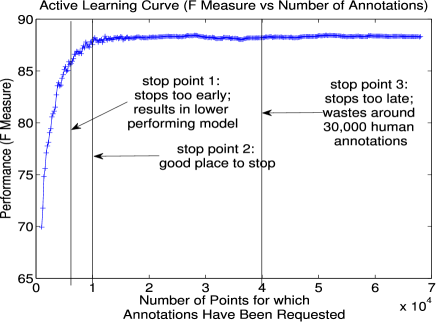
Figure 1: Hypothetical Active Learning Curve with hypothetical stopping points.

The terms aggressive and conservative will be used throughout the rest of this paper to describe the behavior of stopping methods. Conservative methods tend to stop further to the right in Figure 1. They are conservative in the sense that they’re very careful not to risk losing significant amounts of F-measure, even if it means annotating many more examples than necessary. Aggressive methods, on the other hand, tend to stop further to the left in Figure 1. They are aggressively trying to reduce unnecessary annotations.

There has been a flurry of recent work tackling the problem of automatically determining when to stop AL (see Section 2). There are three areas where this body of work can be improved:

applicability

Several of the leading methods are restricted to only being used in certain situations, e.g., they can’t be used with some base learners, they have to select points in certain batch sizes during AL, etc. (See Section 2 for discussion of the exact applicability constraints of existing methods.)

lack of aggressive stopping

The leading methods tend to find stop points that are too far to the right in Figure 1. (See Section 4 for empirical confirmation of this.)

instability

Some of the leading methods work well on some datasets but then can completely break down on other datasets, either stopping way too late and wasting enormous amounts of annotation effort or stopping way too early and losing large amounts of F-measure. (See Section 4 for empirical confirmation of this.)

This paper presents a new stopping method based on stabilizing predictions that addresses each of these areas and provides user-adjustable stopping behavior. The essential idea behind the new method is to test the predictions of the recently learned models (during AL) on examples which don’t have to be labeled and stop when the predictions have stabilized. Some of the main advantages of the new method are that: it requires no additional labeled data, it’s widely applicable, it fills a need for a method which can aggressively save annotations, it has stable performance, and it provides users with control over how aggressively/conservatively to stop AL.

Section 2 discusses related work. Section 3 explains our Stabilizing Predictions (SP) stopping criterion in detail. Section 4 evaluates the SP method and discusses results. Section 5 concludes.

2 Related Work

?) present stopping criteria based on the gradient of performance estimates and the gradient of confidence estimates. Their technique with gradient of performance estimates is only applicable when probabilistic base learners are used. The gradient of confidence estimates method is more generally applicable (e.g., it can be applied with our experiments where we use SVMs as the base learner). This method, denoted by LS2008 in Tables and Figures, measures the rate of change of model confidence over a window of recent points and when the gradient falls below a threshold, AL is stopped.

The margin exhaustion stopping criterion was developed for AL with SVMs (AL-SVM). It says to stop when all of the remaining unlabeled examples are outside of the current model’s margin [Schohn and Cohn, 2000] and is denoted as SC2000 in Tables and Figures. ?) developed a similar technique that stops when the number of support vectors saturates. This is equivalent to margin exhaustion in all of our experiments so this method is not shown explicitly in Tables and Figures. Since we use AL with SVMs, we will compare with margin exhaustion in our evaluation section. Unlike our SP method, margin exhaustion is only applicable for use with margin-based methods such as SVMs and can’t be used with other base learners such as Maximum Entropy, Naive Bayes, and others. ?) show in their experiments that margin exhaustion has a tendency to stop late. This is further confirmed in our experiments in Section 4.

The confidence-based stopping criterion (hereafter, V2008) in [Vlachos, 2008] says to stop when model confidence consistently drops. As pointed out by [Vlachos, 2008], this stopping criterion is based on the assumption that the learner/feature representation is incapable of fully explaining all the examples. However, this assumption is often violated and then the performance of the method suffers (see Section 4).

Two stopping criteria (max-conf and min-err) are reported in [Zhu and Hovy, 2007]. The max-conf method indicates to stop when the confidence of the model on each unlabeled example exceeds a threshold. In the context of margin-based methods, max-conf boils down to be simply a generalization of the margin exhaustion method. Min-err, reported to be superior to max-conf, says to stop when the accuracy of the most recent model on the current batch of queried examples exceeds some threshold (they use 0.9). ?) proposes the use of multi-criteria-based stopping to handle setting the threshold for min-err. They refuse to stop and they raise the min-err threshold if there have been any classification changes on the remaining unlabeled data by consecutive actively learned models when the current min-err threshold is satisfied. We denote this multi-criteria-based strategy, reported to work better than min-err in isolation, by ZWH2008. As seen in [Zhu et al., 2008a], sometimes min-err indeed stops later than desired and ZWH2008 must (by nature of how it operates) stop at least as late as min-err does. The susceptibility of ZWH2008 to stopping late is further shown emprically in Section 4. Also, ZWH2008 is not applicable for use with AL setups that select examples in small batches.

3 A Method for Stopping Active Learning Based on Stabilizing Predictions

To stop active learning at the point when annotations stop providing increases in performance, perhaps the most straightforward way is to use a separate set of labeled data and stop when performance begins to level off on that set. But the problem with this is that it requires additional labeled data which is counter to our original reason for using AL in the first place. Our hypothesis is that we can sense when to stop AL by looking at (only) the predictions of consecutively learned models on examples that don’t have to be labeled. We won’t know if the predictions are correct or not but we can see if they have stabilized. If the predictions have stabilized, we hypothesize that the performance of the models will have stabilized and vice-versa, which will ensure a (much-needed) aggressive approach to saving annotations.

SP checks for stabilization of predictions on a set of examples, called the stop set, that don’t have to be labeled. Since stabilizing predictions on the stop set is going to be used as an indication that model stabilization has occurred, the stop set ought to be representative of the types of examples that will be encountered at application time. There are two conflicting factors in deciding upon the size of the stop set to use. On the one hand, a small set is desirable because then SP can be checked quickly. On the other hand, a large set is desired to ensure we don’t make a decision based on a set that isn’t representative of the application space. As a compromise between these factors, we chose a size of 2000. In Section 4, sensitivity analysis to stop set size is performed and more principled methods for determining stop set size and makeup are discussed.

It’s important to allow the examples in the stop set to be queried if the active learner selects them because they may be highly informative and ruling them out could hurt performance. In preliminary experiments we had made the stop set distinct from the set of unlabeled points made available for querying and we saw performance was qualitatively the same but the AL curve was translated down by a few F-measure points. Therefore, we allow the points in the stop set to be selected during AL.

The essential idea is to compare successive models’ predictions on the stop set to see if they have stabilized. A simple way to define agreement between two models would be to measure the percentage of points on which the models make the same predictions. However, experimental results on a separate development dataset show then that the cutoff agreement at which to stop is sensitive to the dataset being used. This is because different datasets have different levels of agreement that can be expected by chance and simple percent agreement doesn’t adjust for this.

Measurement of agreement between human annotators has received significant attention and in that context, the drawbacks of using percent agreement have been recognized [Artstein and Poesio, 2008]. Alternative metrics have been proposed that take chance agreement into account. In [Artstein and Poesio, 2008], a survey of several agreement metrics is presented. Most of the agreement metrics are of the form:

$$agreement=\frac{A_{o}-A_{e}}{1-A_{e}},$$ (1)

where $A_{o}=$ observed agreement, and $A_{e}=$ agreement expected by chance. The different metrics differ in how they compute $A_{e}$.

The Kappa statistic [Cohen, 1960] measures agreement expected by chance by modeling each coder (in our case model) with a separate distribution governing their likelihood of assigning a particular category. Formally, Kappa is defined by Equation 1 with $A_{e}$ computed as follows:

$$A_{e}=\sum_{k\in\{+1,-1\}}P(k|c_{1})\cdot P(k|c_{2}),$$ (2)

where each $c_{i}$ is one of the coders (in our case, models), and $P(k|c_{i})$ is the probability that coder (model) $c_{i}$ labels an instance as being in category $k$. Kappa estimates $P(k|c_{i})$ based on the proportion of observed instances that coder (model) $c_{i}$ labeled as being in category $k$.

We have found Kappa to be a robust parameter that doesn’t require tuning when moving to a new dataset. On a separate development dataset, a Kappa cutoff of 0.99 worked well. All of the experiments (except those in Table 2) in the current paper used an agreement cutoff of Kappa = 0.99 with zero tuning performed. We will see in Section 4 that this cutoff delivers robust results across all of the folds for all of the datasets.

The Kappa cutoff captures the intensity of the agreement that must occur before SP will conclude to stop. Though an intensity cutoff of K=0.99 is an excellent default (as seen by the results in Section 4), one of the advantages of the SP method is that by giving users the option to vary the intensity cutoff, users can control how aggressive SP will behave. This is explored further in Section 4.

Another way to give users control over stopping behavior is to give them control over the longevity for which agreement (at the specified intensity) must be maintained before SP concludes to stop. The simplest implementation would be to check the most recent model with the previous model and stop if their agreement exceeds the intensity cutoff. However, independent of wanting to provide users with a longevity control, this is not an ideal approach because there’s a risk that these two models could happen to highly agree but then the next model will not highly agree with them. Therefore, we propose using the average of the agreements from a window of the k most recent pairs of models. If we call the most recent model $M_{n}$, the previous model $M_{n-1}$ and so on, with a window size of 3, we average the agreements between $M_{n}$ and $M_{n-1}$, between $M_{n-1}$ and $M_{n-2}$, and between $M_{n-2}$ and $M_{n-3}$. On separate development data a window size of k=3 worked well. All of the experiments (except those in Table 3) in the current paper used a longevity window size of k=3 with zero tuning performed. We will see in Section 4 that this longevity default delivers robust results across all of the folds for all of the datasets. Furthermore, Section 4 shows that varying the longevity requirement provides users with another lever for controlling how aggressively SP will behave.

4 Evaluation and Discussion

4.1 Experimental Setup

We evaluate the Stabilizing Predictions (SP) stopping method on multiple datasets for Text Classification (TC) and Named Entity Recognition (NER) tasks. All of the datasets are freely and publicly available and have been used in many past works.

For Text Classification, we use two publicly available spam corpora: the spamassassin corpus used in [Sculley, 2007] and the TREC spam corpus trec05p-1/ham25 described in [Cormack and Lynam, 2005]. For both of these corpora, the task is a binary classification task and we perform 10-fold cross validation. We also use the Reuters dataset, in particular the Reuters-21578 Distribution 1.0 ModApte split. Since a document may belong to more than one category, each category is treated as a separate binary classification problem, as in [Joachims, 1998, Dumais et al., 1998]. Consistent with [Joachims, 1998, Dumais et al., 1998], results are reported for the ten largest categories. Other TC datasets we use are the 20Newsgroups newsgroup article classification and the WebKB web page classification datasets. For WebKB, as in [McCallum and Nigam, 1998, Zhu et al., 2008a, Zhu et al., 2008b] we use the four largest categories. For all of our TC datasets, we use binary features for every word that occurs in the training data at least three times.

For NER, we use the publicly available GENIA corpus. Our features, based on those from [Lee et al., 2004], are surface features such as the words in the named entity and two words on each side, suffix information, and positional information. We assume a two-phase model where boundary identification has already been performed, as in [Lee et al., 2004].

SVMs deliver high performance for the datasets we use so we employ SVMs as our base learner in the bulk of our experiments (maximum entropy models are used in Subsection 4.3). For selection of points to query, we use the approach that was used in [Tong and Koller, 2002, Schohn and Cohn, 2000, Campbell et al., 2000] of selecting the points that are closest to the current hyperplane. We use SVM^light [Joachims, 1999] for training the SVMs. For the smaller datasets (less than 50,000 examples in total), a batch size of 20 was used with an initial training set of size 100 and for the larger datasets (greater than 50,000 examples in total), a batch size of 200 was used with an initial training set of size 1000.

4.2 Main Results

Table 1 shows the results for all of our datasets. For each dataset, we report the average number of annotations requested by each of the stopping methods as well as the average F-measure achieved by each of the stopping methods.

Task-Dataset	SP	V2008	SC2000	ZWH2008	LS2008	All
TREC-SPAM	2100	56000	3900	29220	3160	56000
(10-fold AVG)	98.33	98.47	98.41	98.44	96.63	98.47
20Newsgroups	678	181	1984	1340	1669	11280
(20-cat AVG)	60.85	18.06	55.43	60.72	54.79	54.81
Spamassassin	326	4362	862	398	1176	5400
(10-fold AVG)	94.57	95.00	95.53	95.94	95.62	95.63
NER-protein	8720	67220	17680	18580	2360	67220
(10-fold AVG)	89.48	90.28	90.38	90.31	76.47	90.28
NER-DNA	4020	67220	10640	7200	3900	67220
(10-fold AVG)	82.40	84.31	84.73	84.51	74.74	84.31
NER-cellType	3840	29600	5540	11580	4580	67220
(10-fold AVG)	86.15	86.87	87.19	87.32	85.65	87.83
Reuters	484	6762	1196	650	1272	9580
(10-cat AVG)	74.29	65.81	73.88	76.77	74.00	75.64
WKB-Course	790	184	1752	912	1740	7420
(10-fold AVG)	83.12	30.34	80.47	83.16	80.55	80.19
WKB-Faculty	808	892	1932	1062	1818	7420
(10-fold AVG)	81.53	40.14	81.79	81.64	81.99	82.36
WKB-Project	646	916	1358	794	1482	7420
(10-fold AVG)	63.30	25.33	58.11	61.82	59.30	61.19
WKB-Student	1258	894	2400	1468	2150	7420
(10-fold AVG)	84.70	50.66	83.46	84.39	83.19	83.30
Average	2152	21294	4477	6655	2301	28509
(macro-avg)	81.70	62.30	80.85	82.27	78.45	81.27

Table 1: Methods for stopping AL. For each dataset, the average number of annotations at the automatically determined stopping points and the average F-measure at the automatically determined stopping points are displayed. Bold entries are statistically significantly different than SP (and non-bold entries are not). The Average row is simply an unweighted macro-average over all the datasets. The final column (labeled ”All”) represents standard fully supervised passive learning with the entire set of training data.

There are two facts worth keeping in mind. First, the numbers in Table 1 are averages and therefore, sometimes two methods could have very similar average numbers of annotations but wildly different average F-measures (because one of the methods was consistently stopping around its average whereas the other was stopping way too early and way too late). Second, sometimes a method with a higher average number of annotations has a lower average F-measure than a method with a lower average number of annotations. This can be caused because of the first fact just mentioned about the numbers being averages and/or this can also be caused by the ”less is more” phenomenon in active learning where often with less data, a higher-performing model is learned than with all the data; this was first reported in [Schohn and Cohn, 2000] and subsequently observed by many others (e.g., [Vlachos, 2008, Laws and Schütze, 2008]).

There are a few observations to highlight regarding the performance of the various stopping methods:

• SP is the most parsimonious method in terms of annotations. It stops the earliest and remarkably it is able to do so largely without sacrificing F-measure.

• All the methods except for SP and SC2000 are unstable in the sense that on at least one dataset they have a major failure, either stopping way too late and wasting large numbers of annotations (e.g. ZWH2008 and V2008 on TREC Spam) or stopping way too early and losing large amounts of F-measure (e.g. LS2008 on NER-Protein) .

• It’s not always clear how to evaluate stopping methods because the tradeoff between the value of extra F-measure versus saving annotations is not clearly known and will be different for different applications and users.

This last point deserves some more discussion. In some cases it is clear that one stopping method is the best. For example, on WKB-Project, the SP method saves the most annotations and has the highest F-measure. But which method performs the best on NER-DNA? Arguments can reasonably be made for SP, SC2000, or ZWH2008 being the best in this case depending on what exactly the annotation/performance tradeoff is. A promising direction for research on AL stopping methods is to develop user-adjustable stopping methods that stop as aggressively as the user’s annotation/performance preferences dictate.

One avenue of providing user-adjustable stopping is that if some methods are known to perform consistently in an aggressive manner against annotating too much while others are known to perform consistently in a conservative manner, then users can pick the stopping criterion that’s more suitable for their particular annotation/performance valuation. For this purpose, SP fills a gap as the other stopping criteria seem to be conservative in the sense defined in Section 1. SP, on the other hand, is more of an aggressive stopping criterion and is less likely to annotate data that is not needed.

A second avenue for providing user-adjustable stopping is a single stopping method that is itself adjustable. To this end, Section 4.3 shows how intensity and longevity provide levers that can be used to control the behavior of SP in a controlled fashion.

Sometimes viewing the stopping points of the various criteria on a graph with the active learning curve can help one visualize how the methods perform. Figure 2 shows the graph for a representative fold. The x-axis measures the number of human annotations that have been requested so far. The y-axis measures performance in terms of F-Measure. The vertical lines are where the various stopping methods would have stopped AL if we hadn’t continued the simulation. The figure reinforces and illustrates what we have seen in Table 1, namely that SP stops more aggressively than existing criteria and is able to do so without sacrificing performance.

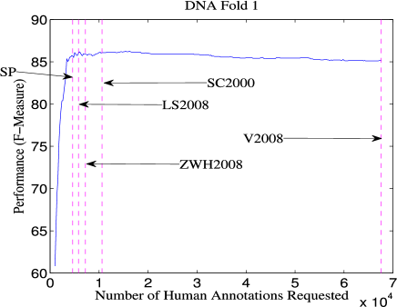
Figure 2: Graphic with stopping criteria in action for fold 1 of NER of DNA from the GENIA corpus. The x-axis ranges from 0 to 70,000.

4.3 Additional Experiments

All of the additional experiments in this subsection were conducted on our least computationally demanding dataset, Spamassassin. The results in Tables 2 and 3 show how varying the intensity cutoff and the longevity requirement, respectively, of SP enable a user to control stopping behavior. Both methods enable a user to adjust stopping in a controlled fashion (without radical changes in behavior). Areas of future work include: combining the intensity and longevity methods for controlling behavior; and developing precise expectations on the change in behavior corresponding to changes in the intensity and longevity settings.

Intensity	Annotations	F-Measure
K=99.5	364	96.01
K=99.0	326	94.57
K=98.5	304	95.59
K=98.0	262	93.75
K=97.5	242	93.35
K=97.0	224	90.91

Table 2: Controlling the behavior of stopping through the use of intensity. For Kappa intensity levels in {97.0, 97.5, 98.0, 98.5, 99.0, 99.5}, the 10-fold average number of annotations at the automatically determined stopping points and the 10-fold average F-measure at the automatically determined stopping points are displayed for the Spamassassin dataset.

Longevity	Annotations	F-Measure
k=1	284	95.17
k=2	318	94.95
k=3	326	94.57
k=4	336	95.40
k=5	346	96.41
k=6	366	94.53

Table 3: Controlling the behavior of stopping through the use of longevity. For window length k longevity levels in {1, 2, 3, 4, 5, 6}, the 10-fold average number of annotations at the automatically determined stopping points and the 10-fold average F-measure at the automatically determined stopping points are displayed for the Spamassassin dataset.

Stop Set Size	Annotations	F-Measure
2500	326	95.58
2000	326	94.57
1500	314	95.00
1000	328	95.73
500	314	94.57

Table 4: Investigating the sensitivity to stop set size. For stop set sizes in {2500, 2000, 1500, 1000, 500}, the 10-fold average number of annotations at the automatically determined stopping points and the 10-fold average F-measure at the automatically determined stopping points are displayed for the Spamassassin dataset.

Task-Dataset	SP	V2008	ZWH2008	LS2008	All
Spamassassin	286	1208	386	756	5400
(10-fold AVG)	94.92	89.89	95.31	96.40	91.74

Table 5: Methods for stopping AL with maximum entropy as the base learner. For each stopping method, the average number of annotations at the automatically determined stopping point and the average F-measure at the automatically determined stopping point are displayed. Bold entries are statistically significantly different than SP (and non-bold entries are not). SC2000, the margin exhaustion method, is not shown since it can’t be used with a non-margin-based learner. The final column (labeled ”All”) represents standard fully supervised passive learning with the entire set of training data.

The results in Table 4 show results for different stop set sizes. Even with random selection of a stop set as small as 500, SP’s performance holds fairly steady. This plus the fact that random selection of stop sets of size 2000 worked across all the folds of all the datasets in Table 1 show that in practice perhaps the simple heuristic of choosing a fairly large random set of points works well. Nonetheless, we think the size necessary will depend on the dataset and other factors such as the feature representation so more principled methods of determining the size and/or the makeup of the stop set are an area for future work. For example, construction techniques could be developed to create stop sets with high representativeness (in terms of feature space) density (meaning representativeness of stop set divided by size of stop set). For example, a possibility is to cluster examples before AL begins and then make sure the stop set contains examples from each of the clusters. Another possibility is to use a greedy algorithm where the stop set is iteratively grown where on each iteration the center of mass of the stop set in feature space is computed and an example in the unlabeled pool that is maximally far in feature space from this center of mass is selected for inclusion in the stop set. This could be useful for efficiency (in terms of getting the same stopping performance with a smaller stop set as could be achieved with a larger stop set) and also as a way to ensure adequate representation of the task space. The latter can be accomplished by perhaps continuing to add examples to the stop set until adding new examples is no longer increasing the representativeness of the stop set.

As one of the advantages of SP is that it’s widely applicable, Table 5 shows the results when using maximum entropy models as the base learner during AL (the query points selected are those which the model is most uncertain about). The results reinforce our conclusions from the SVM experiments, with SP performing aggressively and all statistically significant differences in performance being in SP’s favor. Figure 3 shows the graph for a representative fold.

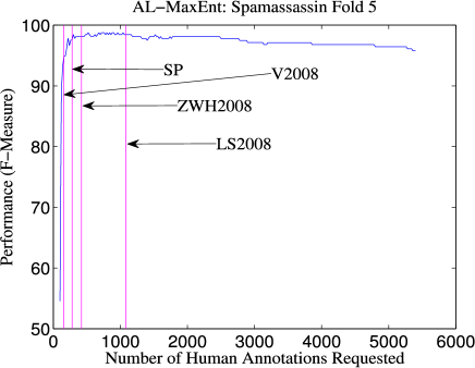
Figure 3: Graphic with stopping criteria in action for fold 5 of TC of the spamassassin corpus. The x-axis ranges from 0 to 6,000.

5 Conclusions

Effective methods for stopping AL are crucial for realizing the potential annotation savings enabled by AL. A survey of existing stopping methods identified three areas where improvements are called for. The new stopping method based on Stabilizing Predictions (SP) addresses all three areas: SP is widely applicable, stable, and aggressive in saving annotations.

The empirical evaluation of SP and the existing methods was informative for evaluating the criteria but it was also informative for demonstrating the difficulties for rigorous objective evaluation of stopping criteria due to different annotation/performance tradeoff valuations. This opens up a future area for work on user-adjustable stopping. Two potential avenues for enabling user-adjustable stopping are a single criterion that is itself adjustable or a suite of methods with consistent differing levels of aggressiveness/conservativeness from which users can pick the one(s) that suit their annotation/performance tradeoff valuation. SP substantially widens the range of behaviors of existing methods that users can choose from. Also, SP’s behavior itself can be adjusted through user-controllable parameters.

References

- [Artstein and Poesio, 2008] Ron Artstein and Massimo Poesio. 2008. Inter-coder agreement for computational linguistics. Computational Linguistics, 34(4):555–596.
- [Baldridge and Osborne, 2008] Jason Baldridge and Miles Osborne. 2008. Active learning and logarithmic opinion pools for hpsg parse selection. Nat. Lang. Eng., 14(2):191–222.
- [Bloodgood and Vijay-Shanker, 2009] Michael Bloodgood and K. Vijay-Shanker. 2009. Taking into account the differences between actively and passively acquired data: The case of active learning with support vector machines for imbalanced datasets. In NAACL.
- [Campbell et al., 2000] Colin Campbell, Nello Cristianini, and Alex J. Smola. 2000. Query learning with large margin classifiers. In ICML ’00: Proceedings of the Seventeenth International Conference on Machine Learning, pages 111–118, San Francisco, CA, USA. Morgan Kaufmann Publishers Inc.
- [Cohen, 1960] J. Cohen. 1960. A coefficient of agreement for nominal scales. Educational and Psychological Measurement, 20:37–46.
- [Cormack and Lynam, 2005] Gordon Cormack and Thomas Lynam. 2005. Trec 2005 spam track overview. In TREC-14.
- [Dumais et al., 1998] Susan Dumais, John Platt, David Heckerman, and Mehran Sahami. 1998. Inductive learning algorithms and representations for text categorization. In CIKM ’98: Proceedings of the seventh international conference on Information and knowledge management, pages 148–155, New York, NY, USA. ACM.
- [Ertekin et al., 2007] Seyda Ertekin, Jian Huang, Léon Bottou, and C. Lee Giles. 2007. Learning on the border: active learning in imbalanced data classification. In Mário J. Silva, Alberto H. F. Laender, Ricardo A. Baeza-Yates, Deborah L. McGuinness, Bjørn Olstad, Øystein Haug Olsen, and André O. Falcão, editors, Proceedings of the Sixteenth ACM Conference on Information and Knowledge Management, CIKM 2007, Lisbon, Portugal, November 6-10, 2007, pages 127–136. ACM.
- [Joachims, 1998] Thorsten Joachims. 1998. Text categorization with suport vector machines: Learning with many relevant features. In ECML, pages 137–142.
- [Joachims, 1999] Thorsten Joachims. 1999. Making large-scale SVM learning practical. In Advances in Kernel Methods – Support Vector Learning, pages 169–184.
- [Laws and Schütze, 2008] Florian Laws and Hinrich Schütze. 2008. Stopping criteria for active learning of named entity recognition. In Proceedings of the 22nd International Conference on Computational Linguistics (Coling 2008), pages 465–472, Manchester, UK, August. Coling 2008 Organizing Committee.
- [Lee et al., 2004] Ki-Joong Lee, Young-Sook Hwang, Seonho Kim, and Hae-Chang Rim. 2004. Biomedical named entity recognition using two-phase model based on svms. Journal of Biomedical Informatics, 37(6):436–447.
- [McCallum and Nigam, 1998] Andrew McCallum and Kamal Nigam. 1998. A comparison of event models for naive bayes text classification. In Proceedings of AAAI-98, Workshop on Learning for Text Categorization.
- [Schohn and Cohn, 2000] Greg Schohn and David Cohn. 2000. Less is more: Active learning with support vector machines. In Proc. 17th International Conf. on Machine Learning, pages 839–846. Morgan Kaufmann, San Francisco, CA.
- [Sculley, 2007] D. Sculley. 2007. Online active learning methods for fast label-efficient spam filtering. In Conference on Email and Anti-Spam (CEAS), Mountain View, CA, USA.
- [Tong and Koller, 2002] Simon Tong and Daphne Koller. 2002. Support vector machine active learning with applications to text classification. Journal of Machine Learning Research (JMLR), 2:45–66.
- [Vlachos, 2008] Andreas Vlachos. 2008. A stopping criterion for active learning. Computer Speech and Language, 22(3):295–312.
- [Zhu and Hovy, 2007] Jingbo Zhu and Eduard Hovy. 2007. Active learning for word sense disambiguation with methods for addressing the class imbalance problem. In Proceedings of the 2007 Joint Conference on Empirical Methods in Natural Language Processing and Computational Natural Language Learning (EMNLP-CoNLL), pages 783–790.
- [Zhu et al., 2008a] Jingbo Zhu, Huizhen Wang, and Eduard Hovy. 2008a. Learning a stopping criterion for active learning for word sense disambiguation and text classification. In IJCNLP.
- [Zhu et al., 2008b] Jingbo Zhu, Huizhen Wang, and Eduard Hovy. 2008b. Multi-criteria-based strategy to stop active learning for data annotation. In Proceedings of the 22nd International Conference on Computational Linguistics (Coling 2008), pages 1129–1136, Manchester, UK, August. Coling 2008 Organizing Committee.