An Estimate of the Spectral Intensity
Expected from the Molecular Bremsstrahlung Radiation
in Extensive Air Showers

Abstract

A detection technique of ultra-high energy cosmic rays, complementary to the fluorescence technique, would be the use of the molecular Bremsstrahlung radiation emitted by low-energy electrons left after the passage of the showers in the atmosphere. The emission mechanism is expected from quasi-elastic collisions of electrons produced in the shower by the ionisation of the molecules in the atmosphere.
In this article, a detailed calculation of the spectral intensity of photons at ground level originating from the transitions between unquantised energy states of free ionisation electrons is presented. In the absence of absorption of the emitted photons in the plasma, the obtained spectral intensity is shown to be $\simeq 4.0\leavevmode\nobreak\ 10^{-26}$ W m^-2 Hz^-1 at 10 km from the shower core for a vertical shower induced by a proton of $10^{17.5}$ eV.

1 Introduction

The origin and nature of ultra-high energy cosmic rays still remain to be elucidated despite the recent progresses provided by the data collected at the Pierre Auger Observatory and the Telescope Array [1]. This is due to the extremely low intensity of particles at these energies. As of today, the most direct way to infer the nature of the particles at ultra-high energies relies on the observation of the shower longitudinal profile to measure its maximum of development. The use of telescopes detecting the nitrogen fluorescence light emitted after the passage of the electromagnetic cascade is a well-suited technique to achieve such measurements. Moreover, these fluorescence telescopes provide a good calorimetric estimate of the energy of the showers, which is preferable to detectors requiring external information to calibrate the energy estimator of the showers. However, this technique can only be used on moonless nights, resulting in a 10% duty cycle. Together with the low intensity of particles, this makes the study of the cosmic ray composition above few tens of EeV very challenging.

Triggered by microwave emission measurements in laboratory [2], new telescope techniques based on the detection of the microwave emission in the GHz C-band (3.4-4.2 GHz) have been developed at the Pierre Auger Observatory [3]. These techniques aim at providing measurements of the electromagnetic content of the cascade with quality comparable to the fluorescence detectors but with a 100% duty cycle. Molecular Bremsstrahlung radiation in the GHz band provides an interesting mechanism to detect ultra-high energy cosmic rays due to the expected isotropic and unpolarised radiation. This feature would allow for the possibility of performing shower calorimetry in the same spirit as the fluorescence technique does, by mapping the ionisation content along the showers through the intensity of the microwave signals detected at ground level.

Attempts to estimate the spectral intensity expected from the molecular Bremsstrahlung radiation in beam experiments [2] or in extensive air showers [4] have been performed, based on general frameworks pertaining to radiative processes in plasmas. In these works, the sources of the emission are the low-energy electrons left along the shower track after the passage of high-energy electrons of the cascade propagating in the atmosphere. The different energy distributions of the ionisation electrons are considered as static during the time the electrons can emit. These approaches resulted in a free-parametric [2] or in a very low expectation [4] for the signal power that could be observed at the ground level.

In this paper, the approach adopted is based on the computation of the spectral power per volume unit, which is shown to be the natural quantity to estimate the spectral intensity at any reference point in space and time. It is derived from the collision rate of ionisation electrons leading to the production of photons through free-free transitions. Moreover, the ionisation electrons are tracked from their production to their disappearance by accounting for all interactions affecting their energy distribution with time, as detailed in section 2. In turn, these electrons can produce their own emission, such as Bremsstrahlung emission. The expected spectral intensity at ground level of such an emission is the object of section 3. Possible attenuation or suppression effects are studied in section 4. Finally, the results obtained in this study are illustrated in section 5 on a toy reference shower. From these results, the perspectives of detection of ultra-high energy cosmic rays by making use of molecular Bremsstrahlung radiation are discussed.

2 Ionisation Electrons along the Shower Track

2.1 A Crude Model of Vertical Air Showers

In this work, an extensive air shower is considered as a thin plane front of high energy charged particles propagating in the atmosphere at the speed of light $c$. For a given primary type and a given energy $E$, the longitudinal development of the electromagnetic cascade depends only on the cumulated slant depth $X$ expressed as the ratio between the vertical thickness of the atmosphere $X_{\mathrm{vert}}$ (1000 g cm^-2 at sea level) and the cosine of the zenith angle of the shower. After the succession of a few initial steps in the cascade, all showers can be described by reproducible macroscopic states. In particular, the shape of the showers is universal except for a translation depending logarithmically on $E$ and a global factor roughly linear in $E$. In this way, for any given slant depth $X$ or equivalently any altitude $a$, the total number of primary $e^{+}/e^{-}$ particles, $N_{e,p}$, can be adequately parameterised by the Gaisser-Hillas function as [5]:

$$N_{e,p}(a)=N_{\mathrm{max}}\bigg{(}\frac{X(a)-X_{0}}{X_{\mathrm{max}}-X_{0}}\bigg{)}^{\frac{X_{\mathrm{max}}-X_{0}}{\lambda}}\exp{\bigg{(}\frac{X_{\mathrm{max}}-X(a)}{\lambda}\bigg{)}},$$ (1)

with $X(a)$ the depth corresponding to the altitude $a$, $X_{0}$ the depth of the first interaction, $X_{\mathrm{max}}$ the depth of shower maximum, $N_{\mathrm{max}}$ the number of particles observed at $X_{\mathrm{max}}$, and $\lambda$ a parameter describing the attenuation of the shower.

On the other hand, high energy particles constituting the core of the shower are collimated along the initial shower axis. The lateral extension of the core depends on the mean free path and can be expressed in terms of the Moliere radius $R_{M}$ such that 90% of the energy is contained within a distance $r$ from the axis such as $r<R_{M}$. Motivated by general arguments to describe the electromagnetic cascade of showers, the NKG lateral distribution function denoted hereafter by $g(r,a)$ is known to reproduce reasonably well the observations [6]:

$$g(r,a)=C(s(a))\leavevmode\nobreak\ R_{M}^{-2}\leavevmode\nobreak\ \left(\frac{r}{R_{M}}\right)^{s(a)-2}\left(1+\frac{r}{R_{M}}\right)^{s(a)-4.5}.$$ (2)

Here, $s(a)$ stands for the age parameter at altitude $a$ defined as $s(a)=3X(a)/(X(a)+2X_{\mathrm{max}})$, and $C(s)$ is a normalisation factor.

Figure 1: Geometry of a vertical shower used throughout the paper.

The number of primary $e^{+}/e^{-}$ per unit surface, $n_{e,p}(r,a)$, is then simply obtained by folding the longitudinal profile to the normalised lateral one. For a vertical shower whose geometry is depicted in figure 1, $n_{e,p}(r,a)$ reads as:

$$n_{e,p}(r,a)=N_{e,p}(a)\leavevmode\nobreak\ \frac{g(r,a)}{2\pi\displaystyle\int\mathrm{d}r\leavevmode\nobreak\ r\leavevmode\nobreak\ g(r,a)}.$$ (3)

Noticeably, this description is only a crude model of an extensive air shower. This shall allow us, however, to derive in the following a realistic number of ionisation electrons left along the shower track and thus to estimate relevant orders of magnitude for the spectral intensities (in W m^-2 Hz^-1) that can be expected from molecular Bremsstrahlung radiation by these ionisation electrons.

To facilitate comparisons of the results obtained in this study with the values reported in [2] and [4], the parameters of both the Gaisser/Hillas and the NKG functions are tuned to apply to vertical proton showers with primary energy $E=10^{17.5}\leavevmode\nobreak\$eV.

2.2 Production of Ionisation Electrons along the Shower Track

Through the passage of charged particles in the atmosphere, the energy of an extensive air shower is deposited mainly through the ionisation process. The resulting numerous ionisation electrons can, in turn, produce their own emission such as continuum Bremsstrahlung emission through quasi-elastic scattering with molecular nitrogen and, to smaller extent, oxygen. To evaluate the spectral intensity of this radiation, we start by deriving below the flux of secondary ionisation electrons created by the development of the shower.

For one single primary electron travelling over an infinitesimal distance $\mathrm{d}a$, and for a mass density $\rho_{m}(a)$ of molecular nitrogen or oxygen, the average number of ionisation electrons per unit length and per kinetic energy band reads as:

$$\frac{\mathrm{d}^{2}N_{e,i}}{\mathrm{d}a\leavevmode\nobreak\ \mathrm{d}T_{e}}(a,T_{e})=\rho_{m}(a)\leavevmode\nobreak\ f_{0}(T_{e})\left\langle\frac{\mathrm{d}E}{\mathrm{d}X}\right\rangle\leavevmode\nobreak\ \frac{1}{I_{0}+\left\langle T_{e}\right\rangle},$$ (4)

with $I_{0}$ the ionisation potential to create an electron-ion pair in air ($I_{0}=15.6\leavevmode\nobreak\$eV for N₂ and $I_{0}=12.1\leavevmode\nobreak\$eV for O₂ molecules). The bracketed expression $\left\langle\frac{\mathrm{d}E}{\mathrm{d}X}\right\rangle$ stands for the mean energy loss of primary electrons per grammage unit. This energy loss is due quasi-exclusively to ionisation and is almost independent of the primary electron energy over a range of few tens of MeV, typical of the primary electrons energy in the cascade. The distribution in kinetic energy of the resulting ionisation electrons is described here by the normalised function $f_{0}(T_{e})$. This distribution has been experimentally determined and accurately parameterised for primary electrons with kinetic energies $T_{e}^{p}$ up to several keV [7]. For higher kinetic energies $T_{e}^{p}$, relativistic effects as well as indistinguishability between primary and secondary electrons have been shown to modify the low-energy behaviour [8]. To account for these effects, we adopt the analytical expression provided in [9]:

$$f_{0}(T_{e})=K\frac{1+C\exp{(-T_{e}/T_{k})}}{T_{e}^{2}+\overline{T}^{2}},$$ (5)

where $T_{e}$ ranges from 0 to $T_{e}^{\mathrm{max}}=(T_{e}^{p}-I_{0})/2$ due to the indistinguishability between primary and secondary electrons, the constant $C$ is determined in the same way as in [7] so that $\int\mathrm{d}T_{e}\leavevmode\nobreak\ C/(T_{e}^{2}+\overline{T}^{2})$ reproduces the total ionisation cross section, $T_{k}=77\leavevmode\nobreak\$eV is a parameter acting as the boundary between close and distant collisions, the constant $K$ is tuned to guarantee $\int\mathrm{d}T_{e}f_{0}(T_{e})=1$, and $\overline{T}=13.0\leavevmode\nobreak\ (17.4)\leavevmode\nobreak\$eV for nitrogen (oxygen). In the energy range of interest, this expression leads to $\left\langle T_{e}\right\rangle\simeq 40\leavevmode\nobreak\$eV, in agreement with the well-known stopping power. The instantaneous number of ionisation electrons per unit volume and per kinetic energy band is then obtained by coupling equation 4 to the number of primary charged particles per surface unit:

$$n_{e,i}^{0}(r,a,T_{e})=\frac{f_{0}(T_{e})}{I_{0}+\left\langle T_{e}\right\rangle}\leavevmode\nobreak\ \left\langle\frac{\mathrm{d}E}{\mathrm{d}X}\right\rangle\leavevmode\nobreak\ \rho_{m}(a)\leavevmode\nobreak\ n_{e,p}(r,a).$$ (6)

Of relevant importance for the following is the flux $\phi_{e,i}^{0}(r,a,T_{e})$ of secondary electrons per kinetic energy band. For any surface element $\mathrm{d}S$, and considering a coordinate system with the zenith angle defined along the axis perpendicular to the surface $\mathrm{d}S$, the total number of electrons $N_{e,i}(r,a,T_{e},\chi,\psi)$ (per kinetic energy band) crossing $\mathrm{d}S$ during a short time interval $dt$ under zenith and azimuth incidence angles $\chi$ and $\psi$ is :

$$N_{e,i}^{0}(r,a,T_{e},\chi,\psi)=c\beta(T_{e})\mathrm{d}t\leavevmode\nobreak\ \int\mathrm{d}\psi\sin{\chi}\mathrm{d}\chi\leavevmode\nobreak\ \mathrm{d}S|\cos{\chi}|\leavevmode\nobreak\ n_{e,i}^{0}(r,a,T_{e},\chi,\psi),$$ (7)

with $\beta(T_{e})$ the relativistic factor. Hereafter, ionisation electrons are considered to be emitted isotropically. This assumption may not be accurate given that ionisation electrons should be produced to some extent along the flow of the general motion of the high-energy electrons of the cascade. However, since low-energy photons will be emitted isotropically from these non-relativistic electrons, this assumption does not impact any of the results concerning the incoherent emission of photons except for a small and irrelevant change of flux of ionisation electrons. Under isotropy, the quantity per solid angle unit $n_{e,i}^{0}(r,a,T_{e},\chi,\psi)$ is independent of the incidence angles and reduces to $n_{e,i}^{0}(r,a,T_{e})/4\pi$. This yields to the expression of the instantaneous flux per kinetic energy band, which is the relevant quantity for the following:

$$\phi_{e,i}^{0}(r,a,T_{e})=\frac{c\beta(T_{e})f_{0}(T_{e})}{2\left\langle I_{0}+T_{e}\right\rangle}\leavevmode\nobreak\ \left\langle\frac{\mathrm{d}E}{\mathrm{d}X}\right\rangle\leavevmode\nobreak\ \rho_{m}(a)\leavevmode\nobreak\ n_{e,p}(r,a).$$ (8)

2.3 Time Evolution of the Flux of Ionisation Electrons

The instantaneous flux per kinetic energy band obtained through equation 8 corresponds to the number of secondary electrons per surface, time and kinetic energy units left just after the passage of the primary high-energy electrons of the shower. The flux of secondary low-energy electrons $\phi_{e,i}(r,a,T_{e},t)$, still per kinetic energy band, available at any time $t$ after the passage of the shower is governed by the interactions that these electrons undergo in the atmosphere. In turn, the evolution in time of the function $\phi_{e,i}(r,a,T_{e},t)$ can be fully encompassed in the time dependence of the distribution in kinetic energy $f(T_{e},t)$ of the ionisation electrons. This evolution is determined by a Boltzmann equation accounting for all the interactions of interest at work, Boltzmann equation that is now detailed and solved numerically.

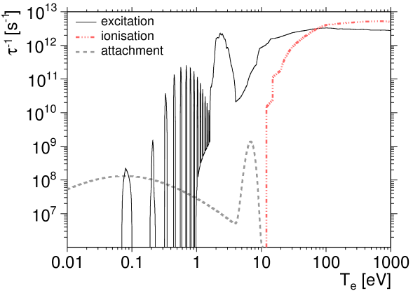
Figure 2: Collision rates of interest as a function of electron kinetic energy, at sea level.

Ionisation electrons can be considered as static in space to a good approximation given their low energy and given that their rate of disappearance is governed by attachment processes which occur on a time scale of at most few hundreds of nanoseconds in the atmospheric layers of interest. It is consequently comfortable to neglect the space diffusion term in the Boltzmann equation. The time evolution of the distribution function $f$ is then exclusively governed by a collision term in the following Boltzmann equation:

$$\frac{\partial f}{\partial t}(T_{e},t) = -n_{m}(a)c\beta(T_{e})\bigg{(}\sigma_{\mathrm{att}}(T_{e})+\sigma_{\mathrm{exc}}(T_{e})+\sigma_{\mathrm{ion}}(T_{e})\bigg{)}f(T_{e},t)$$ (9)

$$+ n_{m}(a)c\int_{T_{e}}^{T_{e}^{\mathrm{max}}}\mathrm{d}T^{\prime}_{e}\beta(T^{\prime}_{e})\bigg{(}\frac{\mathrm{d}\sigma_{\mathrm{ion}}}{\mathrm{d}T_{e}}(T^{\prime}_{e},T_{e})+\frac{\mathrm{d}\sigma_{\mathrm{ion}}}{\mathrm{d}T_{e}}(T^{\prime}_{e},T^{\prime}_{e}-T_{e})\bigg{)}f(T^{\prime}_{e},t)$$

$$+ n_{m}(a)c\int_{T_{e}}^{T_{e}^{\mathrm{max}}}\mathrm{d}T^{\prime}_{e}\beta(T^{\prime}_{e})\frac{\mathrm{d}\sigma_{\mathrm{exc}}}{\mathrm{d}T_{e}}(T^{\prime}_{e},T_{e})f(T^{\prime}_{e},t),$$

where $\sigma_{i}$ denotes the cross sections of interest (ionisation, excitation of electronic levels and attachment processes), and $n_{m}(a)$ is the density of molecules at an altitude $a$ obtained by multiplying the corresponding mass density by the Avogadro number $\mathcal{N}_{A}$ and by dividing by the corresponding molar mass $A$. The first term in the right hand side stands for the disappearance of electrons with kinetic energy $T_{e}$, while the second and third terms stand for the appearance of electrons with kinetic energy $T_{e}$ due to ionisation and excitation (including ro-vibrational excitation) reactions initiated by electrons with higher kinetic energy $T^{\prime}_{e}$. Note that in the case of ionisation, a second electron emerges from the collision with kinetic energy $T^{\prime}_{e}-T_{e}$.

The quantities $\tau^{-1}_{i}=n_{m}(a)c\beta(T_{e})\sigma_{i}(T_{e})$ characterize the rates of collisions. The electron attachment processes with oxygen have been studied in detail as a function of the energy, and is here taken from reference [10]. The corresponding collision rate leads to a characteristic time scale $\tau_{\mathrm{att}}\simeq 20\leavevmode\nobreak\$ns at sea level for energies below 1 eV. The ionisation cross-section is taken from reference [11], it varies between $\simeq 1$ and $\simeq 10$ atomic units in the energy range of interest, leading to a characteristic time scale between two ionisations below $\sim$ 1 picosecond. Finally, collisional rates describing the excitation of the different electronic levels of interest of $O_{2}$ and $N_{2}$ molecules, including ro-vibrational excitation reactions, are taken from [12]. Overall, they lead to characteristic time scales around $\sim$1 picosecond. The different collision rates are shown in figure 2 at sea level. For energies above $\simeq 100\leavevmode\nobreak\$eV, ionisation is the dominant energy loss process, while for energies between $\simeq 1.7$ eV (corresponding to the threshold to excite one of the electronic levels of oxygen) and $100\leavevmode\nobreak\$eV, excitation is the dominant process. Below $\simeq 1.7$ eV, ro-vibrational excitation reactions compete within some quantised energy ranges with the attachment process which causes a real disappearance of electrons.

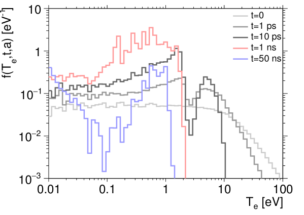
Figure 3: Distribution in kinetic energy of the ionisation electrons at different times (at sea level in this example).

The second and third terms in equation 9 account for the migration of electrons with kinetic energies $T^{\prime}_{e}$ to lower energies through ionisation and excitation processes. From the ionisation collision rate plotted in figure 2, the population of electrons produced with an energy larger than $\simeq 100\leavevmode\nobreak\$eV is expected to be confined in the energy range below $\simeq 100\leavevmode\nobreak\$eV on a time scale much smaller than a nanosecond. New ionisation electrons created through this process undergo the same mechanism. On almost the same time scale, the excitation collision rate is expected to confine all electrons in a small energy window below $\simeq 1.7$ eV. Below this threshold, other excitation processes, mainly ro-vibrational ones, are possible only within quantised energy ranges. Thus, on a larger time scale (from few nanoseconds to a hundred of nanoseconds), the electrons are expected to disappear through the attachment process to oxygen while they shall frequently experience reactions modifying their energy spectrum. To quantify precisely this picture, the Boltzmann equation can be solved numerically in different ways. We show in figure 3 the evolution with time of the function $f$ as obtained by Monte-Carlo for electrons produced at sea level. After few picoseconds only, the energy distribution $f$ is already largely modified by the high collision rate of ionisation for electrons with initial kinetic energies larger than $\simeq 100\leavevmode\nobreak\$eV and by the high collision rate of excitation for electrons with initial kinetic energies smaller than $\simeq 100\leavevmode\nobreak\$eV. After $\simeq 1\leavevmode\nobreak\$ns, all electron energies get below the lowest excitation threshold belonging to the continuous spectrum of energy losses. This results in a sharp cutoff in the $f$ function, which confines all electron energies below $\simeq 1.7\leavevmode\nobreak\$eV on a short time scale. On longer time scales, free electrons can still collide through excitation processes when their energies resonate with the corresponding quantised reactions. This results in a slow drift of the sharp cutoff to lower energies as well as a modification of the shape of the $f$ function. Meanwhile, electrons disappear through the attachment process. Since the number of electrons is not conserved, the normalisation of $f$ against the kinetic energy varies with time; it starts by quickly increasing due to the new electrons produced by ionisation, and then decreases in a quasi-exponential way on a longer time scale driven by the attachment process.

3 Microwave Emission from Molecular Bremsstrahlung: the Free-Free Approach

As long as they remain free, ionisation electrons can produce photons through the process of quasi-elastic collisions with neutral molecules in the atmosphere:

$$e^{\pm}+M\rightarrow e^{\pm}+M+\gamma.$$ (10)

In this approach, the production of photons with energies $h\nu$ corresponds to transitions between unquantised energy states of the free electrons (’free-free’ transitions). The spectral intensity at ground level can be deduced in a straightforward way from the collision rate of ionisation electrons with neutral molecules in air. This approach has been shown to be successful for describing, for instance, the production of free-free radiations in collisions of low energy electrons with neutral atoms in measurements using drift-tube techniques [13].

By considering the production rate $r_{\gamma}$ of photons with energy $h\nu$ per volume unit proportional to the target density only, it is then governed by the electron flux and by the free-free cross section $\sigma_{\mathrm{ff}}(T_{e},h\nu)$, leading to the following expression:

$$r_{\gamma}(r,a,t,\nu)=n_{m}(a)\leavevmode\nobreak\ \int_{0}^{T_{e}^{\mathrm{max}}}\mathrm{d}T_{e}\leavevmode\nobreak\ \phi_{e,i}(r,a,T_{e},t)\leavevmode\nobreak\ \sigma_{\mathrm{ff}}(T_{e},h\nu).$$ (11)

Possible effects of absorption or suppression of the emission due to destructive interferences of the photons within the interaction zone are neglected at this step. Such effects will be further discussed in section 4.

The free-free cross-section as obtained in reference [14] can be related to the electron momentum transfer cross-section through:

$$\sigma_{\mathrm{ff}}(T_{e},h\nu)=\frac{4}{3\pi}\frac{\alpha^{3}}{R_{y}}\left(1-\frac{h\nu}{2T_{e}}\right)\sqrt{1-\frac{h\nu}{T_{e}}}T_{e}\sigma_{m}(T_{e}),$$ (12)

with $\alpha$ the fine-structure constant and $R_{y}$ the Rydberg constant. For electrons with kinetic energies in the range of few tens of eV and photons in the GHz energy range, this expression is very accurately independent of $h\nu$ and can be reduced to $\sigma_{\mathrm{ff}}(T_{e})=1.211\leavevmode\nobreak\ 10^{-8}T_{e}\sigma_{m}(T_{e})$, with $T_{e}$ expressed here in units eV. The electron momentum transfer cross-section, on the other hand, has been well measured on various targets. Compiled tables provided in reference [12] were used for the following.

As already stressed, the space volume that these electrons can probe during their relatively small lifetime is negligible compared to the volume in which an extensive air shower develops. In this way, it is comfortable to consider each electron as a point-like source of photons during its whole lifetime. Hence, from the knowledge of the collision rate per volume unit $r_{\gamma}$, the emitted power per volume unit at each point $(r,a)$ can be simply obtained by coupling this rate to the energy of the emitted photons, so that the emitted spectral power per volume unit can be written as:

$$\frac{\mathrm{d}^{2}P}{\mathrm{d}\nu\mathrm{d}V}(r,a,t) = \frac{\mathrm{d}}{\mathrm{d}\nu}\left(h\nu r_{\gamma}(r,a,t)\right)$$ (13)

$$= \frac{hc\rho_{m}^{2}(a)\mathcal{N}_{A}}{2A(I_{0}+\left\langle T_{e}\right\rangle)}\left\langle\frac{\mathrm{d}E}{\mathrm{d}X}\right\rangle n_{e,p}(r,a)\tilde{\sigma}(t,a),$$ (14)

where $\tilde{\sigma}(t,a)$ is an effective cross-section defined as:

$$\tilde{\sigma}(t,a)=\int_{0}^{T_{e}^{\mathrm{max}}}\mathrm{d}T_{e}f(T_{e},t,a)\beta(T_{e})\sigma_{\mathrm{ff}}(T_{e}).$$ (15)

The transparency to photons of the electrons-neutral molecules will be justified in the next section, so that the radiation produced by individual electrons-nitrogen/oxygen encounters can be considered here to pass out of the interaction volume without absorption or reflection. At any distance $R$, the spectral intensity received from sources contained in any infinitesimal volume $\mathrm{d}V$ is proportional to $\mathrm{d}^{2}P/\mathrm{d}\nu\mathrm{d}V$ times $\mathrm{d}V$ and weighted by $4\pi R^{2}$ given that photons are emitted isotropically from each source. In this way, the observable spectral intensity at any ground position $\mathbf{x}_{g}$, $\Phi_{g}$, is simply the sum of the uncorrelated contributions of the individual encounters:

$$\Phi_{g}(\mathbf{x}_{g},t)=\int_{0}^{\infty}r\mathrm{d}r\int_{0}^{2\pi}\mathrm{d}\varphi\int_{0}^{\infty}\mathrm{d}a\frac{1}{4\pi R^{2}(r,\varphi,a)}\frac{\mathrm{d}^{2}P}{\mathrm{d}\nu\mathrm{d}V}(r,a,t_{d}(t,r,\varphi,a)).$$ (16)

Here, $R$ is the distance between the position at ground $\mathbf{x}_{g}$ and the position of the current source in the integration, and $t_{d}$ is the delayed time at which the emission occurred. Fixing the reference time $t_{0}$ to the time at which the shower front crosses the ground, each source at altitude $a$ started emitting radiation at the time the shower front passed at that altitude (i.e. at $t_{0}-a/c$). Each photon crossing the ground at time $t$ (with the condition that $t\geq t_{0}$) coming from a source at altitude $a$ and located at a distance $r$ from the shower axis was emitted at time $t-Rn(a,\nu)/c$ - with $n(a,\nu)$ the refractive index of the atmosphere integrated along the line of sight between the emission point and the observer. The delayed time $t_{d}(t,r,\varphi,a,\nu)$, denoted hereafter $t_{d}$ only for convenience, is thus expressed as:

$$t_{d}\equiv t_{d}(t,r,\varphi,a,\nu)=t-t_{0}-\left(\frac{R(r,\varphi,a)n(a,\nu)}{c}-\frac{a}{c}\right).$$ (17)

With the evident condition that emissions occur only at $t_{d}\geq 0$, a Heaviside function denoted $\Theta$ is introduced leading to the following semi-analytical expression for the observable spectral intensity:

$$\Phi_{g}(\mathbf{x}_{g},t)=\frac{hc\mathcal{N}_{A}}{8\pi A(I_{0}+\left\langle T_{e}\right\rangle)}\left\langle\frac{\mathrm{d}E}{\mathrm{d}X}\right\rangle\int_{0}^{\infty}r\mathrm{d}r\int_{0}^{2\pi}\mathrm{d}\varphi\int_{0}^{\infty}\mathrm{d}a\leavevmode\nobreak\ \frac{\rho_{m}^{2}(a)n_{e,p}(r,a)}{R^{2}(r,\varphi,a)}\leavevmode\nobreak\ \tilde{\sigma}({t_{d},a})\leavevmode\nobreak\ \Theta(t_{d}).$$ (18)

Besides the free-free approach presented here, an independent estimation of the radiated power using the classical field theory formalism can be applied, resulting in the same predictions. Detailed expressions in this frame can be found in the Appendix.

4 Possible Attenuation Effects in Molecular Bremsstrahlung Radiation

4.1 Absorption Effects

In addition to free-free emissions, ionisation electrons can also experience inverse Bremsstrahlung and stimulated Bremsstrahlung within the electrons-neutral molecules plasma. A convenient way to quantify the size of these effects is to calculate the absorption coefficient, $\alpha_{\nu}$, defined as the relative attenuation per unit length of the emitted photons. The absorption coefficient is defined as the net balance between the number of absorbed photons per unit length subtracted to the number of stimulated emitted photons (due to a photon that causes an electron in the potential of a neutral molecule to emit another photon of the same frequency) per unit length.

To derive the absorption coefficient, it is convenient to introduce the emitted spectral power per volume unit at a fixed energy $T_{e}$, denoted $\eta_{\nu,V}(T_{e},r,a)$, in the same way as in reference [16] for instance. Then, equation 13 can be re-written as:

$$\frac{\mathrm{d}^{2}P}{\mathrm{d}\nu\mathrm{d}V}(r,a,t)=\int\mathrm{d}T_{e}f(T_{e},t,a)\eta_{\nu,V}(T_{e},r,a).$$ (19)

The absorption coefficient $\alpha_{\nu}$ is then known to be related to $\eta_{\nu,V}$ through [16]:

$$\alpha_{\nu}=\frac{c^{2}}{h\nu^{3}}\int\mathrm{d}T_{e}^{\prime}\bigg{[}f_{0}(T_{e},a)-f_{0}(T_{e}^{\prime},a)\bigg{]}\eta_{\nu,V}(T_{e}^{\prime},r,a).$$ (20)

This expression accounts for both the absorption of a photon of energy $h\nu$ by an electron with initial energy $T_{e}$ and a final one $T_{e}^{\prime}$ and the stimulated emission due to a photon that causes a neighboring electron to emit another photon of the same energy within the electrons-neutral molecules plasma. Given the low frequencies of the photons considered here compared to the mean energy of the electrons, expanding $f_{0}(T_{e},a)$ to first order in energy leads to:

$$f_{0}(T_{e}^{\prime},a)=f_{0}(T_{e},a)+h\nu\frac{\partial f_{0}}{\partial T_{e}^{\prime}},$$ (21)

so that the absorption coefficient $\alpha_{\nu}$ reads as:

$$\alpha_{\nu}(r,a)=-\frac{c^{2}}{\nu^{2}}\int\mathrm{d}T_{e}\frac{\partial f_{0}(T_{e},a)}{\partial T_{e}}\eta_{\nu,V}(T_{e},r,a).$$ (22)

Injecting explicitly the expression of $\eta_{\nu,V}$ into this expression, $\alpha_{\nu}$ turns out to read:

$$\alpha_{\nu}(r,a)=-\frac{hc^{3}\rho^{2}(a)\mathcal{N}_{A}}{2A(I_{0}+\left\langle T_{e}\right\rangle)}\frac{1}{\nu^{2}}\left\langle\frac{\mathrm{d}E}{\mathrm{d}X}\right\rangle n_{e,p}(r,a)\int\mathrm{d}T_{e}\beta(T_{e})\sigma_{\mathrm{ff}}(T_{e})\frac{\partial f_{0}(T_{e},a)}{\partial T_{e}}.$$ (23)

Close to the shower core and to the maximum of shower development (that is, within the denser plasma region), this leads to $\nu^{2}\alpha_{\nu}\simeq 10^{-4}$ m^-1 Hz². At GHz frequencies, the absorption is thus negligible.

4.2 Suppression Effects

The spectral intensity predicted by equation 18 is based on the assumption that the emitted radiation passes out of the interaction volume without undergoing any dispersive properties of the plasma caused by the successive interactions of the electrons.

Dispersive properties are commonly described on a macroscopic basis by a dielectric coefficient. This coefficient allows a derivation of the absorption coefficient which, in contrast to the previous derivation, accounts for successive collisions within the radiation formation zone of each electron-neutral collision. The effect of the successive collisions, known as the plasma dispersion effect [16], can lead to destructive interferences of the radiated fields.

Accounting for the coupling of electrons to the emitted radiation turns out to be a difficult task here, since it consists in considering an additional term in equation 9 proportional to $\partial f/\partial T_{e}$ times the radiated electric fields. To get an order of magnitude of the effects which might be at work, we adopt the commonly used method consisting in linearising a simplified Boltzmann equation pertaining only to the case of a distribution function $f(T_{e})$ stationary in time in the absence of any emitted radiation. In this case, it can be shown that the plasma dispersion effects result in a suppression factor in the integrand of $\tilde{\sigma}$ defined in equation 15 reading as [16]:

$$\frac{1}{1+(\nu_{c}(T_{e},t)/\nu)^{2}},$$ (24)

where $\nu_{c}(T_{e},t)$ is the time-dependent rate of inelastic collisions of the electrons of kinetic energy $T_{e}$. From the analysis of section 2.3, this collision rate amounts to several THz within the first nanosecond for highly energetic electrons and then decreases to the level of a few tens of MHz. Consequently, for frequencies $\nu$ around the GHz, the suppression factor can be important only during the first nanosecond, as long as the collision rate is much larger than the frequency considered for the radiation field.

It is to be noted that the suppression factor aforementioned is derived by means of a series of hypotheses which are not really relevant in the case considered here. However, it is clear that such plasma dispersion effects can be important only when $\nu_{c}(T_{e},t)$ is larger than $\nu$. As a kind of proxy to probe these effects in the most pessimistic way, the impact can be evaluated by suppressing the emission as long as $\nu_{c}(T_{e},t)>\nu$.

5 Discussion

Although semi-analytical integrations of equation 18 are possible without random number generators, a Monte-Carlo sampling of the integrand function in $r$ and $\varphi$ allows a much faster integration in terms of CPU time. Results presented here have thus been obtained using random number generators to carry out these particular integrations.

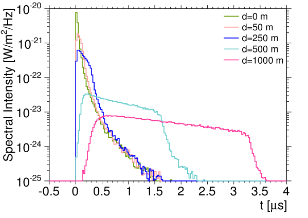
Figure 4: Spectral intensity as a function of time expected at different distances from the shower core at ground level, for a vertical shower with energy $10^{17.5}$ eV.

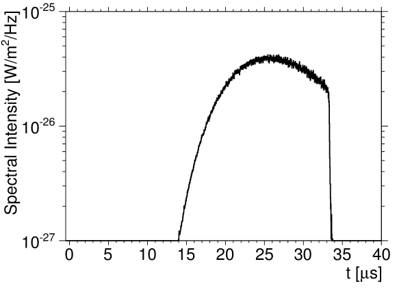
Figure 5: Spectral intensity as a function of time expected at 10 km from the shower core at ground level, for a vertical shower with energy $10^{17.5}$ eV.

A vertical proton shower of $10^{17.5}$ eV is used as a proxy to illustrate the estimation of the spectral intensity expected from molecular Bremsstrahlung radiation presented in section 3. The parameterisation of the atmosphere selected here is the widely used US standard atmosphere, based on experimental data [18]. The parameterisation of the wavelength dependence of the refractive index is taken from [19].

Experimental setups using regularly spaced antennas oriented vertically or nearly vertically detect showers crossing the field-of-view and impacting the ground. The spectral intensity expected at different distances from the shower core at ground level as derived from equation 18 is shown in figure 4. This figure is relevant for the case of the currently running EASIER installation at the Pierre Auger Observatory [3] or for the CROME experiment [20]. It is seen that the spectral intensity is rapidly decreasing in amplitude for increasing distances to the shower core. The duration of the signals at different distances can be understood from the characteristic time scale of the attachment process on the one hand, and from the different regions of the shower that can be probed for different positions at ground on the other hand. This result is in disagreement with expectations found in [4], in which the signal time profiles at these distances are difficult to interpret when accounting for all-interaction cross sections. Furthermore, the reported short signal duration and the low amplitudes are not found to be reproducible by considering only the attachment process as in [4], .

An alternative detection method of microwave radiation is the use of large aperture receivers pointing just above the horizon to observe the longitudinal profiles of the showers at large distances, such as MIDAS and AMBER installations at the Pierre Auger observatory [3, 21]. The received power as a function of time at a distance of 10 km from the shower axis is shown in figure 5. It turns out to be $\simeq 4.0\leavevmode\nobreak\ 10^{-26}$ W m^-2 Hz^-1. To probe the maximal impact of the plasma dispersion effects as discussed in the previous section, the same simulation is repeated with the condition of suppressing the emission as long as $\nu_{c}(T_{e},t)>\nu$. At 10 km from the shower axis, the signal is found to be $\simeq 3.8\leavevmode\nobreak\ 10^{-26}$ W m^-2 Hz^-1, not significantly different from the spectral intensity value obtained without accounting for any suppression effect. This gives an idea about the small systematic uncertainty which affects the estimate due to possible collective suppression within the plasma.

The estimated intensity is found to be smaller than the one reported in reference [2] by a factor $\simeq 70$ when scaling the beam measurements to air showers. Recent results from [24] reported a measurement of an anisotropic distribution of the molecular Bremsstrahlung radiation. The interpretation of this result in the frame of air shower physics is not yet clear and needs further investigation. We note that results from laboratory measurements are still to be confirmed by independent experiments [22, 23].

In air shower experiments, an important difficulty arises from the separation power between the molecular Bremsstrahlung radiation signals and signals due to the geomagnetic radiation. Close to the shower core, the measured signal amplitude from geomagnetic radiation [20] is greater than or of the same order as the one expected from molecular Bremsstrahlung radiation found in this study. However, the expected signal duration appears significantly larger (about a factor 100) comparing to the measured signal from geomagnetic radiation. Together with the unpolarised nature of the signal, there are thus possible experimental signatures for the molecular Bremsstrahlung radiation which would allow its identification, provided that the experimental setup is sensitive enough. Based on this study, significant increases in sensitivity should thus be achieved from an experimental point of view to be able to detect showers induced by ultra-high energy cosmic rays by means of the molecular Bremsstrahlung emission mechanism.

Classical Field theory approach in Molecular Bremsstrahlung Radiation estimation

From the point of view of the classical field theory, the radiated power by the ionisation electrons is associated to the deviations caused by the collisions with the neutral molecules. In this framework, although the formal expression of the spectral intensity expected at ground level is unchanged with respect to equation 16, the expression of the emitted spectral power per volume unit has to be revised to remove any reference to free-free transitions.

Figure 6: Geometry of a classical binary collision. The vector change in velocity is $|\Delta\mathbf{v}|=2v\sin{(\chi/2)}$.

In a classical way, when an electron approaches a neutral molecule, the electric field of the electron polarises the neutral molecule. This polarisation gives rise to a dipole moment which induces an attractive interaction potential at a short distance range : $V(d)\propto d^{-4}$ - with $d$ the distance between the electron and the molecule. The time-dependent radiated power during the interaction is known to obey the Larmor formula : $p_{e}(t)=e^{2}\left|\dot{\mathbf{v}}(t)\right|^{2}/6\pi\epsilon_{0}c^{3}$, with $e$ the elementary charge and $\epsilon_{0}$ the vacuum permittivity. Then, by making use of the Parseval identity, one can derive directly the frequency spectrum of the radiated energy for one collision as:

$$\frac{\mathrm{d}E}{\mathrm{d}\nu}(\nu,v,\chi)=\frac{e^{2}}{3\pi\epsilon_{0}c^{3}}\left|\int_{-\infty}^{\infty}\mathrm{d}t\leavevmode\nobreak\ \dot{\mathbf{v}}(t)\exp{(-i2\pi\nu t)}\right|^{2}.$$ (25)

Since the interaction potential acts at a short distance range only, the average time during which the interaction is taking place can be estimated as $\Delta t\simeq b/\left<v\right>$, with $b$ the impact parameter of the collision. For typical electron velocities of the order of a few percents of the speed of light, a realistic order of magnitude for $\Delta t$ is $\simeq 10^{-16}\leavevmode\nobreak\$s so that for GHz frequencies, $2\pi\nu\tau\ll 1$ for any $\tau$ within $\Delta t$ . Hence, the argument in the exponential of the integrand is very small during the time where the electron is accelerated, so that for an electron undergoing a total deviation by an angle $\chi$, the corresponding frequency spectrum of the radiated energy can be accurately estimated as:

$$\frac{\mathrm{d}E}{\mathrm{d}\nu}(v,\chi) = \frac{e^{2}}{3\pi\epsilon_{0}c^{3}}\left|\Delta\mathbf{v}\right|^{2}$$ (26)

$$= \frac{2e^{2}}{3\pi\epsilon_{0}c^{3}}v^{2}(1-\cos{\chi}),$$ (27)

where the expression of $\left|\Delta\mathbf{v}\right|$ has been easily derived from the geometry of the collision depicted in figure 6.

The collision rate per volume unit, per electron velocity band and per solid angle unit (with here $d\Omega=\sin{\chi}d\chi d\psi$) is governed by the same ingredients as in the previous section, except that the free-free cross-section is now replaced by the classical differential cross-section:

$$\frac{\mathrm{d}^{2}r_{\gamma}^{\mathrm{cl}}}{\mathrm{d}v\mathrm{d}\Omega}(r,a,t,v,\chi)=n_{m}(a)\leavevmode\nobreak\ \phi_{e,i}(r,a,v,t)\leavevmode\nobreak\ \frac{\mathrm{d}\sigma^{\mathrm{cl}}}{\mathrm{d}\Omega}(v,\chi),$$ (28)

where the flux of ionisation electrons is now expressed, for convenience, per velocity band instead of kinetic energy band. This is achieved by expressing the kinetic energy in terms of the velocity and by substituting the normalised $f$ function by the one obtained through the relevant Jacobian transformation:

$$\tilde{f}(v,t)=\frac{m_{e}v}{(1-(v/c)^{2})^{3/2}}f(T_{e}(v),t).$$ (29)

Since the collision rate is independent of the frequency, the emitted spectral power per volume unit can be obtained by integrating this collision rate directly coupled to the frequency spectrum of the energy radiated per collision over solid angle and the velocity $v$. This leads to:

$$\frac{\mathrm{d}^{2}P^{\mathrm{cl}}}{\mathrm{d}\nu\mathrm{d}V}(r,a,t)=\frac{e^{2}\rho_{m}^{2}(a)\mathcal{N}_{A}}{3\pi\epsilon_{0}A(I_{0}+\left\langle T_{e}\right\rangle)}\left\langle\frac{\mathrm{d}E}{\mathrm{d}X}\right\rangle\leavevmode\nobreak\ n_{e,p}(r,a)\leavevmode\nobreak\ \tilde{\sigma}^{\mathrm{cl}}(t,a),$$ (30)

with the classical effective cross-section defined as:

$$\tilde{\sigma}^{\mathrm{cl}}(t,a)=\int\mathrm{d}v\leavevmode\nobreak\ \tilde{f}(v,t)\left(\frac{v}{c}\right)^{3}\int\mathrm{d}\Omega\leavevmode\nobreak\ (1-\cos{\chi})\frac{\mathrm{d}\sigma^{\mathrm{cl}}}{\mathrm{d}\Omega}(v,\chi).$$ (31)

Note that the result of the solid angle integration is, by definition, the momentum transfer cross-section $\sigma_{m}(T_{e}(v))$.

Hence, it is clear by identification that equation 30 can be equivalent to equation 13 only if the following correspondence holds :

$$hc\tilde{\sigma}(t,a)\rightarrow\frac{2e^{2}}{3\pi\epsilon_{0}}\tilde{\sigma}^{\mathrm{cl}}(t,a).$$ (32)

And, it turns out that both energy volumes equal, for nitrogen targets, $t=1\leavevmode\nobreak\$ns and at sea level for instance, to $\simeq 4.5\leavevmode\nobreak\ 10^{-37}$ eV m³. Given the low energy of the photons considered here compared to the electron energies, the classical approach results in the same prediction as the free-free approach.

References

References

- [1] see e.g. K. H. Kampert, P. Tinyakov, C. R. Physique 15 (2014) 318
- [2] P. W. Gorham et al., Phys. Rev. D78 (2008) 032007
- [3] R. Gaior for the Pierre Auger Collaboration, arXiv:1307.5059, Proceedings of 33rd ICRC (2013), id 0883
- [4] P. Neunteufel et al., Proceedings of 33rd ICRC, id 1220
- [5] T. K. Gaisser, A. M. Hillas, Proceedings of 15th ICRC (1977) Vol 8, 353
- [6] K. Greisen, Progress in Cosmic Ray Physics 3 (1956) North Holland Publ.; K. Kamata, J. Nishimura, Prog. Theoret. Phys. Suppl. 6 (1958) 93
- [7] C. B. Opal et al., J. Chem. Phys. 55 (1971) 4100
- [8] J. Rosado, F. Blanco and F. Arqueros, Astropart. Phys. 55 (2014) 51
- [9] F. Arqueros, F. Blanco and J. Rosado, New Journal of Physics 11 (2009) 065011
- [10] N. Kroll, K. N. Watson, Phys. Rev. A 5 (1972) 1883
- [11] D. Rapp, P. Englander-Golden, J. Chem. Phys. 43 (1965) 1464
-
[12]
A. V. Phelps et al., JILA cross-sections,
http://jila.colorado.edu/ avp/collision_data/electronneutral/ELECTRON.TXT - [13] C. Yamabe, S. J. Buckman, A. V. Phelps, Phys. Rev. A27 (1983) 1345
- [14] V. Kas’yanov, A. Starostin, Sov. Phys.-JETP 21 (1961) 193
- [15] see e.g. L. Landau & E. Lifchitz, Quantum Electrodynamics, Ed MIR, 1973
- [16] G. Bekefi, Radiation Processes in Plasmas, John Wiley and sons, Inc., New-York, 1966
- [17] S. Chandrasekhar , Radiative Transfer, Dover publications, Inc., New-York, 1960
- [18] NASA, NOAA and US Air Force, US standard atmosphere 1976, NASA technical report NASA- TM-X-74335, NOAA technical report NOAA-S/T-76-1562 (1976)
- [19] R. C. Weast (ed.), Handbook of Chemistry and Physics, 67th edition, E373, The Chemical Rubber Co., Cleveland (1986)
- [20] R. Smida et al., Phys. Rev. Lett. 113 (2014) 22, 221101
- [21] J. Alvarez-Muniz et al., Nucl. Instrum. Meth. A 719 (2013) 70
- [22] M. Monasor et al., arXiv:1108.6321, Proceedings of 32nd ICRC (2011), Vol 3, 196
- [23] J. Alvarez-Muniz et al., arXiv:1310.4662, PoS (EPS-HEP 2013) 026
- [24] E. Conti, G. Collazuol, G. Sartori, Phys. Rev. D 90 (2014) 071102(R)