Taking into Account the Differences between Actively and Passively Acquired Data: The Case of Active Learning with Support Vector Machines for Imbalanced Datasets

Abstract

Actively sampled data can have very different characteristics than passively sampled data. Therefore, it’s promising to investigate using different inference procedures during AL than are used during passive learning (PL). This general idea is explored in detail for the focused case of AL with cost-weighted SVMs for imbalanced data, a situation that arises for many HLT tasks. The key idea behind the proposed InitPA method for addressing imbalance is to base cost models during AL on an estimate of overall corpus imbalance computed via a small unbiased sample rather than the imbalance in the labeled training data, which is the leading method used during PL.

1 Introduction

Recently there has been considerable interest in using active learning (AL) to reduce HLT annotation burdens. Actively sampled data can have different characteristics than passively sampled data and therefore, this paper proposes modifying algorithms used to infer models during AL. Since most AL research assumes the same learning algorithms will be used during AL as during passive learning (PL), this paper opens up a new thread of AL research that accounts for the differences between passively and actively sampled data.

The specific case focused on in this paper is that of AL with SVMs (AL-SVM) for imbalanced datasets. Collectively, the factors: interest in AL, widespread class imbalance for many HLT tasks, interest in using SVMs, and PL research showing that SVM performance can be improved substantially by addressing imbalance, indicate the importance of the case of AL with SVMs with imbalanced data.

Extensive PL research has shown that learning algorithms’ performance degrades for imbalanced datasets and techniques have been developed that prevent this degradation. However, to date, relatively little work has addressed imbalance during AL (see Section 2). In contrast to previous work, this paper advocates that the AL scenario brings out the need to modify PL approaches to dealing with imbalance. In particular, a new method is developed for cost-weighted SVMs that estimates a cost model based on overall corpus imbalance rather than the imbalance in the so far labeled training data. Section 2 discusses related work, Section 3 discusses the experimental setup, Section 4 presents the new method called InitPA, Section 5 evaluates InitPA, and Section 6 concludes.

2 Related Work

A problem with imbalanced data is that the class boundary (hyperplane) learned by SVMs can be too close to the positive (pos) examples and then recall suffers. Many approaches have been presented for overcoming this problem in the PL setting. Many require substantially longer training times or extra training data to tune parameters and thus are not ideal for use during AL. Cost-weighted SVMs (cwSVMs), on the other hand, are a promising approach for use with AL: they impose no extra training overhead. cwSVMs introduce unequal cost factors so the optimization problem solved becomes:

Minimize:

$$\frac{1}{2}\|\vec{w}\|^{2}+C_{+}\sum_{i:y_{i}=+1}\xi_{i}+C_{-}\sum_{i:y_{i}=-1}\xi_{i}\vspace*{-.4cm}$$ (1)

Subject to:

$$\forall k:y_{k}\left[\vec{w}\cdot\vec{x}_{k}+b\right]\geq 1-\xi_{k},$$ (2)

where $(\vec{w},b)$ represents the learned hyperplane, $\vec{x}_{k}$ is the feature vector for example $k$, $y_{k}$ is the label for example $k$, $\xi_{k}=max(0,1-y_{k}(\vec{w}_{k}\cdot\vec{x}_{k}+b))$ is the slack variable for example $k$, and $C_{+}$ and $C_{-}$ are user-defined cost factors.

The most important part for this paper are the cost factors $C_{+}$ and $C_{-}$. The ratio $\frac{C_{+}}{C_{-}}$ quantifies the importance of reducing slack error on pos train examples relative to reducing slack error on negative (neg) train examples. The value of the ratio is crucial for balancing the precision recall tradeoff well. [Morik et al., 1999] showed that during PL, setting $\frac{C_{+}}{C_{-}}=\frac{\mbox{\# of neg training examples}}{\mbox{\# of pos training examples}}$ is an effective heuristic. Section 4 explores using this heuristic during AL and explains a modified heuristic that could work better during AL.

[Ertekin et al., 2007] propose using the balancing of training data that occurs as a result of AL-SVM to handle imbalance and do not use any further measures to address imbalance. [Zhu and Hovy, 2007] used resampling to address imbalance and based the amount of resampling, which is the analog of our cost model, on the amount of imbalance in the current set of labeled train data, as PL approaches do. In contrast, the InitPA approach in Section 4 bases its cost models on overall (unlabeled) corpus imbalance rather than the amount of imbalance in the current set of labeled data.

3 Experimental Setup

We use relation extraction (RE) and text classification (TC) datasets and SVM^light [Joachims, 1999] for training the SVMs. For RE, we use AImed, previously used to train protein interaction extraction systems ([Giuliano et al., 2006]). As in previous work, we cast RE as a binary classification task (14.94% of the examples in AImed are positive). We use the $K_{GC}$ kernel from [Giuliano et al., 2006], one of the highest-performing systems on AImed to date and perform 10-fold cross validation. For TC, we use the Reuters-21578 ModApte split. Since a document may belong to more than one category, each category is treated as a separate binary classification problem, as in [Joachims, 1998]. As in [Joachims, 1998], we use the ten largest categories, which have imbalances ranging from 1.88% to 29.96%.

4 AL-SVM Methods for Addressing Class Imbalance

The key question when using cwSVMs is how to set the ratio $\frac{C_{+}}{C_{-}}$. Increasing it will typically shift the learned hyperplane so recall is increased and precision is decreased (see Figure 1 for a hypothetical example). Let PA$=\frac{C_{+}}{C_{-}}$. How should the PA be set during AL-SVM?

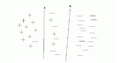
Figure 1: Hyperplane B was trained with a higher $\frac{C_{+}}{C_{-}}$ ratio than hyperplane A was trained with.

We propose two approaches: one sets the PA based on the level of imbalance in the labeled training data and one aims to set the PA based on an estimate of overall corpus imbalance, which can drastically differ from the level of imbalance in actively sampled training data. The first method is called CurrentPA, depicted in Figure 2. Note that in step 0 of the loop, PA is set based on the distribution of positive and negative examples in the current set of labeled data. However, observe that during AL the ratio $\frac{\mbox{\# neg labeled examples}}{\mbox{\# pos labeled examples}}$ in the current set of labeled data gets skewed from the ratio in the entire corpus because AL systematically selects the examples that are closest to the current model’s hyperplane and this tends to select more positive examples than random selection would select (see also [Ertekin et al., 2007]).

Input:
	$L=$ small initial set of labeled data
	$U=$ large pool of unlabeled data
Loop until stopping criterion is met:
	0. Set PA $=\frac{|\{x\in Labeled:f(x)=-1\}|}{|\{x\in L:f(x)=+1\}|}$
	where $f$ is the function we desire to learn.
	1. Train an SVM with $C_{+}$ and $C_{-}$ set such
	that $\frac{C_{+}}{C_{-}}=$ PA and obtain hyperplane $h\;.$
	2. $batch\leftarrow$ select k points from $U$ that are
	closest to $h$ and request their labels.
	3. $U=U-batch\;.$
	4. $L=L\cup batch\;.$
End Loop

Figure 2: The CurrentPA algorithm

Empirical evidence of this distribution skew is illustrated in Figure 3. The trend toward balanced datasets during AL could mislead and cause us to underestimate the PA.

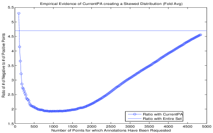
Figure 3: Illustration of AL skewing the distribution of pos/neg points on AImed.

Therefore, our next algorithm aims to set the PA based on the ratio of neg to pos instances in the entire corpus. However, since we don’t have labels for the entire corpus, we don’t know this ratio. But by using a small initial sample of labeled data, we can estimate this ratio with high confidence. This estimate can then be used for setting the PA throughout the AL process. We call this method of setting the PA based on a small initial set of labeled data the InitPA method. It is like CurrentPA except we move Step 0 to be executed one time before the loop and then use that same PA value on each iteration of the AL loop.

To guide what size to make the initial set of labeled data, one can determine the sample size required to estimate the proportion of positives in a finite population to within sampling error $e$ with a desired level of confidence using standard statistical techniques found in many college-level statistics references such as [Berenson et al., 1988]. For example, carrying out the computations on the AImed dataset shows that a size of 100 enables us to be 95% confident that our proportion estimate is within 0.0739 of the true proportion. In our experiments, we used an initial labeled set of size 100.

5 Evaluation

In addition to InitPA and CurrentPA, we also implemented the methods from [Ertekin et al., 2007, Zhu and Hovy, 2007]. We implemented oversampling by duplicating points and by BootOS [Zhu and Hovy, 2007]. To avoid cluttering the graphs, we only show the highest-performing oversampling variant, which was by duplicating points. Learning curves are presented in Figures 4 and 5.

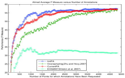
Figure 4: AImed learning curves. y-axis is from 20% to 60%.

Figure 5: Reuters learning curves. y-axis is from 76% to 83%.

Note InitPA is the highest-performing method for all datasets, especially in the practically important area of where the learning curves begin to plateau. This area is important because this is around where we would want to stop AL [Bloodgood and Vijay-Shanker, 2009].

Observe that the gains of InitPA over CurrentPA are smaller for Reuters. For some Reuters categories, InitPA and CurrentPA have nearly identical performance. Applying the models learned by CurrentPA at each round of AL on the data used to train the model reveals that the recall on the training data is nearly 100% for those categories where InitPA/CurrentPA perform similarly. Increasing the relative penalty for slack error on positive training points will not have much impact if (nearly) all of the pos train points are already classified correctly. Thus, in situations where models are already achieving nearly 100% recall on their train data, InitPA is not expected to outperform CurrentPA.

The hyperplanes learned during AL-SVM serve two purposes: sampling - they govern which unlabeled points will be selected for human annotation, and predicting - when AL stops, the most recently learned hyperplane is used for classifying test data. Although all AL-SVM approaches we’re aware of use the same hyperplane at each round of AL for both of these purposes, this is not required. We compared InitPA with hybrid approaches where hyperplanes trained using an InitPA cost model are used for sampling and hyperplanes trained using a CurrentPA cost model are used for predicting, and vice-versa, and found that InitPA performed better than both of these hybrid approaches. This indicates that the InitPA cost model yields hyperplanes that are better for both sampling and predicting.

6 Conclusions

We’ve made the case for the importance of AL-SVM for imbalanced datasets and showed that the AL scenario calls for modifications to PL approaches to addressing imbalance. For AL-SVM, the key idea behind InitPA is to base cost models on an estimate of overall corpus imbalance rather than the class imbalance in the so far labeled data. The practical utility of the InitPA method was demonstrated empirically; situations where InitPA won’t help that much were made clear; and analysis showed that the sources of InitPA’s gains were from both better sampling and better predictive models.

InitPA is an instantiation of a more general idea of not using the same inference algorithms during AL as during PL but instead modifying inference algorithms to suit esoteric characteristics of actively sampled data. This is an idea that has seen relatively little exploration and is ripe for further investigation.

References

- [Berenson et al., 1988] Mark L. Berenson, David M. Levine, and David Rindskopf. 1988. Applied Statistics. Prentice-Hall, Englewood Cliffs, NJ.
- [Bloodgood and Vijay-Shanker, 2009] Michael Bloodgood and K. Vijay-Shanker. 2009. A method for stopping active learning based on stabilizing predictions and the need for user-adjustable stopping. In CoNLL.
- [Ertekin et al., 2007] Seyda Ertekin, Jian Huang, Léon Bottou, and C. Lee Giles. 2007. Learning on the border: active learning in imbalanced data classification. In CIKM.
- [Giuliano et al., 2006] Claudio Giuliano, Alberto Lavelli, and Lorenza Romano. 2006. Exploiting shallow linguistic information for relation extraction from biomedical literature. In EACL.
- [Joachims, 1998] Thorsten Joachims. 1998. Text categorization with suport vector machines: Learning with many relevant features. In ECML, pages 137–142.
- [Joachims, 1999] Thorsten Joachims. 1999. Making large-scale SVM learning practical. In Advances in Kernel Methods – Support Vector Learning, pages 169–184.
- [Morik et al., 1999] Katharina Morik, Peter Brockhausen, and Thorsten Joachims. 1999. Combining statistical learning with a knowledge-based approach - a case study in intensive care monitoring. In ICML, pages 268–277.
- [Zhu and Hovy, 2007] Jingbo Zhu and Eduard Hovy. 2007. Active learning for word sense disambiguation with methods for addressing the class imbalance problem. In EMNLP-CoNLL.