Atomic correlation energies and the generalized gradient approximation

Abstract

Careful extrapolation of atomic correlation energies suggests that $E_{\scriptscriptstyle\rm C}\to-AZlnZ+BZ$ as $Z\to\infty$, where $Z$ is the atomic number, $A$ is known, and $B$ is about 38 milliHartrees. The coefficients roughly agree with those of the high-density limit of the real-space construction of the generalized gradient approximation. An asymptotic coefficient, missed by previous derivations, is included in a revised approximation. The exchange is also corrected, reducing atomic errors considerably.

Modern density functional theory (DFT) is applied to a huge variety of molecules and materials with many impressive resultsPribram-Jones et al. (2014). But hundreds of different approximations are availableMarques et al. (2012), many of which contain empirical parameters that have been optimized over some set of training dataBecke (1993); Lee et al. (1988). The most popular non-empirical approximations are those of Perdew and co-workers, which eschew empiricism in favor of exact conditions using only the uniform and slowly-varying electron gases for input. But even this non-empirical approach can require judicious choice among exact conditionsHaas et al. (2010), which can appear at odds with claims of DFT being first-principlesPribram-Jones et al. (2014).

A unified, systematic approach to functional approximation is possible. Lieb and SimonLieb and Simon (1973) showed that the ground-state energy in Thomas-Fermi (TF) theory becomes relatively exact in a specific high-density, large particle number limit. In a peculiar sense the density, $n({\bf r})$, also approaches that of TF Lieb (1981). For model systems, the leading corrections to TF, derived semiclassically, have been shown to be much more accurate than typical density functional approximationsElliott et al. (2008). The simplest example of this limit is $Z\to\infty$ for neutral atoms, where the local density approximation (LDA) to the exchange energy, $E_{\scriptscriptstyle\rm X}$, becomes relatively exactSchwinger (1981). Some modern generalized gradient approximations (GGA’s) yield the leading energetic correctionPerdew et al. (2006); Elliott and Burke (2009). While such limits themselves do not wholly determine approximations, they do indicate precisely which limits a non-empirical approximation must satisfyHaas et al. (2010). Understanding of this limit was key to the PBEsol approximation that was designed to improve lattice parameters in solidsPerdew et al. (2008).

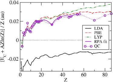
Figure 1: Atomic correlation energies per electron, with the leading large-$Z$ contribution removed. Accurate quantum chemical (QC) results (see text) and approximate self-consistent DFT results.

Here, we extend this idea to correlation, and ask: Does LDA yield the dominant term, and should GGA recover the leading correction? From GGA, we derive a simple formula for the large-$Z$ correlation energy of atoms. Reference quantum chemical (QC) energies for spherical atomsMcCarthy and Thakkar (2011) match this form, and asymptotic coefficients can be extracted numerically. We find that the real-space cutoff construction of a GGA roughly reproduces this number, validating both that procedureBurke et al. (1997) and the seminal idea of Ma and BrucknerMa and Brueckner (1968). Fig. 1 shows non-empirical GGAs like PBE are highly accurate in this limit, while empirical formulas such as LYPLee et al. (1988) fail.

Taking advantage of this insight, we explore the behavior of the GGA at large $Z$, finding an important new condition for correlation. A new approximation is created that satisfies this condition. To test this form, we fill in atomic correlation energies over more of the periodic table, by performing random phase appoximation (RPA) calculations for non-spherical atoms up to Xe, and correct them to yield accurate correlation energies. The errors of the new approximation across periods are consistent with its semiclassical derivation, and are smaller by a factor of 2 than those of PBE. A related correction to the PBE exchange then yields errors smaller by a factor of 4. These results indisputably tie the uniform and slowly-varying gases to real systems.

We begin our analysis with the uniform electron gas (jellium). In a landmark of electronic structure theory, Gell-Mann and BruecknerGell-Mann and Brueckner (1957) applied the random phase approximation (RPA) to find:

$$\epsilon_{\scriptscriptstyle\rm C}^{\rm unif}=c_{0}\ \ln r_{s}-c_{1}+...,~{}~{}~{}r_{\scriptscriptstyle\rm S}\to 0$$ (1)

where $r_{\scriptscriptstyle\rm S}=(3/(4\pi n))^{1/3}$ is the Wigner-Seitz radius of density $n$, $c_{0}=0.031091$, and $c_{1}^{\rm RPA}=0.07082$. We use atomic units (energies in Hartrees) and give derivations for spin-unpolarized systems for simplicity, but all calculations include spin-polarization, unless otherwise noted. Our aim is to find the non-relativistic limit and all results are for this case. In fact, Eq. (1) yields the exact high-density limit if $c_{1}=0.04664$, the correction from RPA being due to second-order exchange. An accurate modern parametrization that contains these limits is given in Ref. Perdew and Wang (1992a). ThenKohn and Sham (1965)

$$E_{\scriptscriptstyle\rm C}^{\rm LDA}[n]=\int d^{3}r\,n({\bf r})\ \epsilon_{\scriptscriptstyle\rm C}^{\rm unif}(n({\bf r})),$$ (2)

which greatly overestimates the magnitude of the correlation energy of atoms (factor of 2 or more). For atoms with large $Z$, insert $n^{\rm TF}({\bf r})$ into Eq. (2) to find:

$$E_{\scriptscriptstyle\rm C}^{\rm LDA}=-AZ\,\ln Z\,+B^{\rm LDA}Z+...,$$ (3)

where $A=2c_{0}/3=0.02072$ and $B^{\rm LDA}=-0.00451$. The first term is exact for atomsKunz and Rueedi (2010), so we define

$$B=\lim_{Z\to\infty}(E_{\scriptscriptstyle\rm C}(Z)/Z+A\ln Z).$$ (4)

Fig. 1 suggests $B$ is finite, undefined in LYP, finite but inaccurate in LDA, and roughly correct in PBE.

To understand why PBE should be accurate, we review the history of non-empirical GGAs. Again within RPA, Ma and Brueckner (MB) derive the leading gradient correction for the correlation energy of a slowly varying electron gasMa and Brueckner (1968). Defining

$$\Delta E_{\scriptscriptstyle\rm C}=E_{\scriptscriptstyle\rm C}-E_{\scriptscriptstyle\rm C}^{\rm LDA},$$ (5)

the gradient expansion approximation yields

$$\Delta\epsilon_{\scriptscriptstyle\rm C}^{\rm GEA}({\bf r})=\beta\,t^{2}({\bf r}),~{}~{}~{}~{}~{}(r_{\scriptscriptstyle\rm S}\to 0)$$ (6)

where $t=|\nabla n|/(2k_{s}n)$ is the dimensionless gradient for correlation, $\beta=0.066725$ and $k_{\scriptscriptstyle\rm S}=2(3n/\pi)^{1/6}$ is the TF screening lengthPerdew et al. (1996). This so strongly overcorrects $E_{\scriptscriptstyle\rm C}^{\rm LDA}$ for atoms that some $E_{\scriptscriptstyle\rm C}$ become positive. MB showed that a simple Pade approximant works much better, creating the first modern GGA, and inspiring the work of Langreth and PerdewLangreth and Perdew (1980), among others.

But underlying some GGAs is the non-empirical real-space cutoff (RSC) procedure for the XC holeBurke et al. (1997). Write

$$E_{\scriptscriptstyle\rm XC}=\frac{1}{2}\int d^{3}r\,\int d^{3}r^{\prime}\,\frac{n({\bf r})\,n_{\scriptscriptstyle\rm XC}({\bf r},{\bf r}^{\prime})}{|{\bf r}-{\bf r}^{\prime}|}.$$ (7)

The LDA can be considered as approximating the true XC hole by that of a uniform gas:

$$n_{\scriptscriptstyle\rm XC}^{\rm LDA}({\bf r},{\bf r}^{\prime})=n({\bf r})\,(\bar{g}^{\rm unif}(r_{\scriptscriptstyle\rm S}({\bf r}),|{\bf r}-{\bf r}^{\prime}|)-1)$$ (8)

where $\bar{g}^{\rm unif}$ is the (coupling-constant averaged) pair-correlation function of the uniform gasPerdew and Wang (1992b). Insertion of this approximate hole into Eq. (7) yields $E_{\scriptscriptstyle\rm XC}^{\rm LDA}[n]$. While $e_{\scriptscriptstyle\rm XC}^{\rm unif}(n({\bf r}))$ is not accurate point-wiseJones and Gunnarsson (1989), the system- and spherical average of the LDA hole is. This is because the LDA hole satisfies some basic conditions (normalized to -1 and $n_{\scriptscriptstyle\rm X}({\bf r},{\bf r}^{\prime})\leq 0$), so it roughly mimics the exact hole. Hence the reliability and systematic errors of LDA Jones and Gunnarsson (1989).

This analysis shows why the gradient expansion fails: $n_{\scriptscriptstyle\rm XC}^{\rm GEA}$ for a non-slowly varying system has large unphysical corrections to $n_{\scriptscriptstyle\rm XC}^{\rm LDA}$, violating the exact conditionsBurke et al. (1998). The RSC construction sharply cuts off the parts of the hole that violate these conditions. The PBE functional is a parametrization of RSC and the paper also showed how the basic features could be deduced by restraining simple forms with exact conditionsPerdew et al. (1996). Its form for correlation is

$$\Delta\epsilon_{\scriptscriptstyle\rm C}^{\rm PBE}(r_{\scriptscriptstyle\rm S},t)=c_{0}\,\ln\left[1+\beta\,t^{2}\,F(\tilde{A}t^{2})/c_{0}\right],$$ (9)

where $F=(1+x)/(1+x+x^{2})$, and

$$\beta\tilde{A}^{-1}=c_{0}\left[\exp(-\epsilon_{\scriptscriptstyle\rm C}^{\rm unif}/c_{0})-1\right].$$ (10)

This form yields a finite $E_{\scriptscriptstyle\rm C}$ in the high-density limit of finite systems, zero correlation as $t\to\infty$, and recovers the gradient expansion for small $t$, just as RSC doesPerdew et al. (1996).

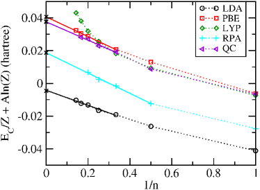
Figure 2: Same as Fig 1, but plotted against inverse principal quantum number, and using only noble gases. Solid lines are straight-line extrapolations to estimate $B$ of Eq. (4).

Everything discussed so far is long known. Our analysis begins by noting that accurate values of $B$ cannot be extracted directly from Fig. 1. The extrapolation to $Z\to\infty$ is obscured by the oscillations across the periodic table. Using methods developed in Ref. Constantin et al. (2010), in Fig. 2 we include only noble gases and plot as a function of inverse principal quantum number. By linear extrapolation, we find $B$ is about 0.038 for QC, and 0.0406 for PBE. The analogous plots for alkali earths give asymptotes 1 to 2 milliHartree higher. We can also find $B^{\rm PBE}$ analytically. As $r_{\scriptscriptstyle\rm S}\to 0$, $\tilde{A}\to 0$ and $F\to 1$, yielding

$$\Delta\epsilon_{\scriptscriptstyle\rm C}^{\rm PBE}(0,t)=c_{0}\,\ln(1+\beta t^{2}/c_{0}).$$ (11)

Inserting an accurateLee et al. (2009) $n^{\rm TF}({\bf r})$ yields $B^{\rm PBE}=0.0393$ exactlyPerdew et al. (2006). The agreement within a few milliHartree validates the extrapolation.

We pause to discuss the message of Figs 1 and 2. First, the original idea of MB, that of resumming the gradient expansion, is validated, but the real-space construction for the correlation hole is needed. Second, the LDA and RSC determine the correlation energies of atoms for large $Z$, explaining their relevance to atomic and molecular systems. Third, the large-$Z$ expansion determines which conditions in functional construction ensure accurate energies. Any approximation, such as LYP, which does not produce the $AZ\ln Z$ dependence, worsens with increasing $Z$: LYP is not optimal even for 3d transition metal complexesFurche and Perdew (2006).

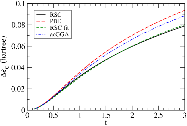
Figure 3: $\Delta\epsilon_{\scriptscriptstyle\rm C}(0,t)$ for real-space cutoff (RSC), PBE, our fit to RSC, and the asymptotically correct GGA (acGGA).

The accuracy of $B^{\rm PBE}$ suggests the real-space cut-off procedure is highly accurate here. To check this, we derive RSC in the large-$Z$ limit. Appendix C of Ref. Burke et al. (1997) gives formulas for RSC as $r_{\scriptscriptstyle\rm S}\to 0$. Solving the RSC equations numerically, we find Fig. 3, which compares PBE and RSC for the high-density limit. The result is rather surprising. Although PBE follows RSC almost perfectly for $t<1/2$, they clearly differ for large $t$. They both have the same $\ln t$ divergence for large $t$, but differ in the next order. Define

$$C=\lim_{t\to\infty}(\Delta\epsilon^{\rm GGA}_{\scriptscriptstyle\rm C}(0,t)-2c_{0}\,\ln t),$$ (12)

to find $C^{\rm PBE}=c_{0}\ln(\beta/c_{0})=0.0237$. For the real-space construction, define

$$\gamma=\lim_{\epsilon\to 0}\int_{\epsilon}^{\infty}dv\,\frac{f_{1}(v)-4c_{0}}{2v},$$ (13)

where $v=k_{\scriptscriptstyle\rm S}u$ and $f_{1}(v)$ is the dimensionless radial $n_{\scriptscriptstyle\rm C}^{\rm LDA}(u)$ in RPA. Then

$$C^{\rm RSC}=c_{0}(3-2\ln(3\pi{\sqrt{6c_{0}}}))+\gamma,$$ (14)

which is about -0.0044 with the models of Ref. Burke et al. (1997). We use this to fit the RSC curve with a simple form:

$$\Delta\epsilon_{\scriptscriptstyle\rm C}^{\rm RSC}(0,t)=c_{0}\,\ln\left[1+\beta t^{2}P(t)/c_{0}\right]$$ (15)

where $P(t)=(1+t/\tau)/(1+\tilde{c}t/\tau)$, $c_{0}\ln\tilde{c}=C^{\rm PBE}-C^{\rm RSC}$, and $\tau=4.5$ is chosen to match the RSC curve. This satisfies all the conditions of PBE correlation, plus one more: it contains the RSC leading correction to $\ln t$, unlike PBE. Then $B^{\rm RSC}=0.0327$. The difference from PBE is small, because $t$ is $<1$ for most of the TF atom (see Fig 9 of Ref. Lee et al. (2009)), reflecting the uncertainty in RSC in this limit.

To construct an approximation without this uncertainty, we keep $\tau$ the same, but choose $\tilde{c}_{\scriptscriptstyle\rm AC}\!=\!1.467$, which reproduces our best estimate of $B$. Our asymptotically corrected GGA (acGGA) is then

$$\Delta\epsilon_{\scriptscriptstyle\rm C}^{\rm acGGA}(r_{s},t)=c_{0}\,\ln\left[1+\beta\tilde{t}^{2}F(\tilde{t}^{2})/c_{0}\right].$$ (16)

where $\tilde{t}=t\sqrt{P(t)}$. acGGA satisfies all the conditions of PBE correlation, but also reproduces the correct large-$Z$ behavior for atoms. Unlike other suggestionsZhang and Yang (1998); Perdew et al. (2008), this is not a change of the constants in the PBE form, but a new form without which this condition cannot be satisfied.

We need more data to test and understand our approximation: $Z$ up to 18Chakravorty et al. (1993) is too far from the asymptotic region, and the spherical atoms aloneMcCarthy and Thakkar (2011) are too sparse. For $19\leq Z\leq 54$ we have performed RPA calculations, evaluating the coupling constant integration using the fluctuation-dissipation theorem at imaginary frequency. We used the optimized effective potential $v_{\text{LEXX}}({\bf r})$ for the linear exact exchange (LEXX)Gould and Dobson (2013a) functional (found via the Krieger, Li and Iafrate approximationKrieger et al. (1992)). Even for open-shell systems $v_{\text{LEXX}}({\bf r})$ is independent of both spin and angle, and includes important features of the exact potential due to its inclusion of static correlation. Details can be found in Refs. Gould and Dobson, 2013a, b, and its extension to $d$ shells via ensemble averagingPerdew et al. (1982) will be discussed in a longer paper. We then fit the correction:

$$E^{\rm QC}\approx E^{\rm RPA}+Z(0.0199+0.00246/n(Z)+...)$$ (17)

where $n(Z)=(6Z+8)^{1/3}-2$. This agrees almost exactly with spherical atoms in the range $19\leq Z\leq 54$ (Fig. 1), and with all atoms in $11\leq Z\leq 18$, another illustration of the power of asymptotic analysis. All energies are listed in Supplementary Information.

	$E_{\scriptscriptstyle\rm C}$					$E_{\scriptscriptstyle\rm XC}$
p	RPA+	LDA	LYP	PBE	ac	PBE	b88-ac	ac
1	0.035	0.765	0.012	0.081	0.094	0.216	0.038	0.034
2	0.074	0.941	0.038	0.069	0.053	0.287	0.071	0.032
3	0.020	1.032	0.045	0.041	0.013	0.297	0.024	0.103
4	0.010	1.000	0.085	0.111	0.062	0.357	0.018	0.113
5	0.020	1.087	0.103	0.049	0.008	0.428	0.009	0.087
all	0.026	1.019	0.089	0.074	0.038	0.365	0.025	0.086

Table 1: Mean absolute error (eV) of energy components per electron, taken with respect to our reference data set, and averaged over each period (p) of the periodic table.

The left side of Table 1 lists average errors for atomic correlation with respect to this reference set. LDA overestimates by about 1 eV per electron, consistent with its error for $B$. PBE reduces this error by about a factor of 10, consistent with its (almost) exact value for $B$. acGGA reduces this error by a further factor of 2, by being exact for $B$. The nefarious LYP does best for $Z<10$, vital to organic chemistry, but is far worse past period 3. Even RPA+Kurth and Perdew (1999), which requires RPA correlation energies, is only slightly better than acGGA.

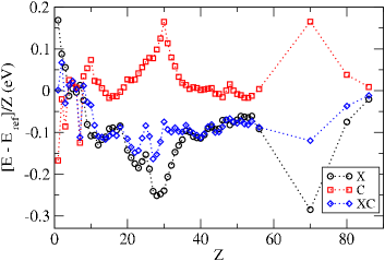
Figure 4: Errors in energy components per electron as a function of $Z$ for acGGA for X, C, and XC together. PBE errors are significantly larger (see Table 1) and do not often cancel.

We close by applying the same methodology to $E_{\scriptscriptstyle\rm X}$. In Ref. Elliott and Burke (2009), it was shown that both B88Becke (1988) and PBE are asymptotically accurate for $E_{\scriptscriptstyle\rm X}$. But close inspection of Table 1 of Ref. Elliott and Burke (2009) shows a small underestimate in the coefficient from PBE. To correct this, we simply increase $\mu$ in the formula for $E_{\scriptscriptstyle\rm X}^{\rm PBE}$ by 13%, to 0.249. We combine this with our correlation approximation to make acGGA, and plot XC energy errors per electron in Fig. 4. Remarkably, the bad actors ($Z=10,30,70$) are the same for both X and C. To understand why these are bad, note that the semiclassical expansion performs worst when only the lowest level of a spatial orbital is occupiedCangi et al. (2010). Writing $n({\bf r})$ as a sum over contributions from different $l$-values, the bad actors are those at which a new $l$-shell has been filled for the first time (2p, 3d, 4f, respectively). A small energy error per electron keeps adding until that shell is filled. No such error occurs in the following period, so that even periods have much large acGGA errors than odd periods in Table 1. The X and C errors are like mirror images, so that they somewhat cancel each other, just as in LDA. This is reflected in the right side of Table 1. For XC together, the acGGA MAE is less than a quarter of PBE’s. In fairness, we note that the empirical B88 exchange functional is so asymptotically accurate that, combined with acGGA correlation, its error is three times smaller again.

Our results are quite general. Lieb-Simon scaling can be applied to any system, if bond lengths are also scaledLieb (1981). TF energies become relatively exact, and we believe LDA X and C both do too. We expect $B^{\rm acGGA}$ to be highly accurate for molecules and solids, so our acGGA for XC may well prove more accurate than PBE for more than just atoms.

KB and SP thank NSF CHE-1112442 for support. SP acknowledges funding by the European Commission (Grant No. FP7-NMP-CRONOS). TG recognises computing support from the Griffith University Gowonda HPC Cluster. No empirical parameters were used in the construction of the approximation suggested here. Explicit formulas are given in Supplemental Information, and a more detailed account is in preparation.

References

- Pribram-Jones et al. (2014) A. Pribram-Jones, D. A. Gross, and K. Burke, Annual Review of Physical Chemistry (2014).
- Marques et al. (2012) M. A. Marques, M. J. Oliveira, and T. Burnus, Computer Physics Communications 183, 2272 (2012).
- Becke (1993) A. D. Becke, The Journal of Chemical Physics 98, 5648 (1993).
- Lee et al. (1988) C. Lee, W. Yang, and R. G. Parr, Phys. Rev. B 37, 785 (1988).
- Haas et al. (2010) P. Haas, F. Tran, P. Blaha, L. S. Pedroza, A. J. R. da Silva, M. M. Odashima, and K. Capelle, Phys. Rev. B 81, 125136 (2010).
- Lieb and Simon (1973) E. Lieb and B. Simon, Phys. Rev. Lett. 31, 681 (1973).
- Lieb (1981) E. H. Lieb, Rev. Mod. Phys. 53, 603 (1981).
- Elliott et al. (2008) P. Elliott, D. Lee, A. Cangi, and K. Burke, Phys. Rev. Lett. 100, 256406 (2008).
- Schwinger (1981) J. Schwinger, Phys. Rev. A 24, 2353 (1981).
- Perdew et al. (2006) J. P. Perdew, L. A. Constantin, E. Sagvolden, and K. Burke, Phys. Rev. Lett. 97, 223002 (2006).
- Elliott and Burke (2009) P. Elliott and K. Burke, Can. J. Chem. Ecol. 87, 1485 (2009).
- Perdew et al. (2008) J. P. Perdew, A. Ruzsinszky, G. I. Csonka, O. A. Vydrov, G. E. Scuseria, L. A. Constantin, X. Zhou, and K. Burke, Physical Review Letters 100, 136406 (2008).
- McCarthy and Thakkar (2011) S. P. McCarthy and A. J. Thakkar, The Journal of Chemical Physics 134, 044102 (2011).
- Burke et al. (1997) K. Burke, J. P. Perdew, and Y. Wang, “Derivation of a generalized gradient approximation: The pw91 density functional,” in Electronic Density Functional Theory: Recent Progress and New Directions, edited by J. F. Dobson, G. Vignale, and M. P. Das (Plenum, NY, 1997) p. 81.
- Ma and Brueckner (1968) S.-K. Ma and K. Brueckner, Phys. Rev. 165, 18 (1968).
- Gell-Mann and Brueckner (1957) M. Gell-Mann and K. Brueckner, Phys. Rev. 106, 364 (1957).
- Perdew and Wang (1992a) J. P. Perdew and Y. Wang, Phys. Rev. B 45, 13244 (1992a).
- Kohn and Sham (1965) W. Kohn and L. J. Sham, Phys. Rev. 140, A1133 (1965).
- Kunz and Rueedi (2010) H. Kunz and R. Rueedi, Phys. Rev. A 81, 032122 (2010).
- Perdew et al. (1996) J. P. Perdew, K. Burke, and M. Ernzerhof, Phys. Rev. Lett. 77, 3865 (1996), ibid. 78, 1396(E) (1997).
- Langreth and Perdew (1980) D. C. Langreth and J. P. Perdew, Phys. Rev. B 21, 5469 (1980).
- Perdew and Wang (1992b) J. P. Perdew and Y. Wang, Phys. Rev. B 46, 12947 (1992b).
- Jones and Gunnarsson (1989) R. Jones and O. Gunnarsson, Rev. Mod. Phys. 61, 689 (1989).
- Burke et al. (1998) K. Burke, J. P. Perdew, and M. Ernzerhof, The Journal of Chemical Physics 109, 3760 (1998).
- Constantin et al. (2010) L. A. Constantin, J. C. Snyder, J. P. Perdew, and K. Burke, The Journal of Chemical Physics 133, 241103 (2010).
- Lee et al. (2009) D. Lee, L. A. Constantin, J. P. Perdew, and K. Burke, J. Chem. Phys. 130, 034107 (2009).
- Furche and Perdew (2006) F. Furche and J. Perdew, J. Chem. Phys. 124, 044103 (2006).
- Zhang and Yang (1998) Y. Zhang and W. Yang, Phys. Rev. Lett. 80, 890 (1998).
- Chakravorty et al. (1993) S. J. Chakravorty, S. R. Gwaltney, E. R. Davidson, F. A. Parpia, and C. F. Fischer, Phys. Rev. A 47, 3649 (1993).
- Gould and Dobson (2013a) T. Gould and J. F. Dobson, The Journal of Chemical Physics 138, 014103 (2013a).
- Krieger et al. (1992) J. B. Krieger, Y. Li, and G. J. Iafrate, Phys. Rev. A 45, 101 (1992).
- Gould and Dobson (2013b) T. Gould and J. F. Dobson, The Journal of Chemical Physics 138, 014109 (2013b).
- Perdew et al. (1982) J. P. Perdew, R. G. Parr, M. Levy, and J. L. Balduz, Phys. Rev. Lett. 49, 1691 (1982).
- Kurth and Perdew (1999) S. Kurth and J. P. Perdew, Phys. Rev. B 59, 10461 (1999).
- Becke (1988) A. D. Becke, Phys. Rev. A 38, 3098 (1988).
- Cangi et al. (2010) A. Cangi, D. Lee, P. Elliott, and K. Burke, Phys. Rev. B 81, 235128 (2010).