Perturbation-based inference for diffusion processes: Obtaining effective models from multiscale data

Abstract.

We consider the inference problem for parameters in stochastic differential equation models from discrete time observations (e.g. experimental or simulation data). Specifically, we study the case where one does not have access to observations of the model itself, but only to a perturbed version which converges weakly to the solution of the model. Motivated by this perturbation argument, we study the convergence of estimation procedures from a numerical analysis point of view. More precisely, we introduce appropriate consistency, stability, and convergence concepts and study their connection. It turns out that standard statistical techniques, such as the maximum likelihood estimator, are not convergent methodologies in this setting, since they fail to be stable. Due to this shortcoming, we introduce and analyse a novel inference procedure for parameters in stochastic differential equation models which turns out to be convergent. As such, the method is particularly suited for the estimation of parameters in effective (i.e. coarse-grained) models from observations of the corresponding multiscale process. We illustrate these theoretical findings via several numerical examples.

Keywords. stochastic differential equation, parametric inference, perturbed observation, convergence, consistency, stability, coarse-graining

AMS subject classifications. 60H10, 60J60, 62M05, 34E13, 60H30, 65R32, 62F20, 62F12

1. Introduction

Stochastic differential equation (SDE) models play a prominent role when studying the temporal evolution of diverse phenomena arising in a wide range of areas. In many applications it is desirable to fit an SDE model to discrete time observations (e.g. experimental or simulation data) of the phenomenon of interest in order to use this model for further analysis [Krumscheid2015-PhysRevE]. It is often possible to justify postulating an SDE model with a particular structure based on theoretical arguments or previous experience with related systems. In that case fitting the model to the available discrete time observations corresponds to determining an unknown parameter vector $\theta\in\mathbb{R}^{n}$ that characterises an $d$-dimensional SDE model such as

(1) $$dX=f(X;\theta)\,dt+g(X;\theta)\,dW\;.$$

In abstract terms, an estimator for $\theta$ can be viewed as a mapping from the sample space (i.e. the space of observations) to the parameter space $\mathbb{R}^{n}$ and it is solely derived from model (1). For concreteness, let the observations of $X$ correspond to model (1) with true parameter $\theta$ and denote by $\Lambda_{\lambda}(X)$ the estimated value using the procedure $\Lambda_{\lambda}$ based on these observations. Here $\lambda$ is a generic parameter which accounts for effects that influence the estimated value, such as the number of discrete time observations or effects due to other approximations. Of particular interest is to verify that the parameter vector $\theta$ can be recovered asymptotically from the observations, i.e. it is desirable that $\lim_{\lambda\rightarrow 0}\Lambda_{\lambda}(X)=\theta$ in an appropriate sense, with $\lambda\rightarrow 0$ denoting a generic limit value. For instance, if $\Lambda_{\lambda}(X)$ denotes the continuous time maximum likelihood estimator based on the observed path $X$ over the time interval $[0,T]$ (we will come back to this estimator in Section 2.1), then we wish to recover the true parameter asymptotically as $T\rightarrow\infty$, so that $\lambda=1/T$ in this case. There exists a vast and well-established literature concerning this property, both from theoretical and computational aspects [PrakasaRao1999, Kutoyants2004, Iacus2008, Liptser2010]. For the special case of estimating parameters in ordinary differential equations, i.e. $g\equiv 0$ in equation (1), see [Li2005] for example.

In this work, we are interested in a slightly different scenario: instead of having direct access to observations $X$ corresponding to model (1) with true parameter $\theta$, we only observe a process $X^{\varepsilon}$ which converges weakly to $X$ in the limit of $\varepsilon\rightarrow 0$. This situation cannot easily be ruled out in many practical applications. One such example is the problem of inferring effective coarse-grained models from observations of a complex or possibly unknown system with multiple temporal and/or length scales. These multiscale systems (both deterministic and stochastic) emerge naturally in a range of applications, including biology [Chauviere2010], atmosphere and ocean sciences [Majda2008], molecular dynamics [Griebel2007], materials science [Fish2009], and fluid and solid mechanics [Horstemeyer2010, Huerre1998]. For such a multiscale system with, e.g., two widely separated time scales one typically only has access to discretely sampled observations of the multiscale process $X^{\varepsilon}$ which converges weakly in $C([0,T],\mathbb{R}^{d})$ to the solution $X$ of the corresponding coarse-grained model as $\varepsilon\rightarrow 0$. Nevertheless one is interested in identifying parameters in the coarse-grained model solved by $X$ using the observation $X^{\varepsilon}$. In other examples one might, however, not even be aware of the fact that one observes only a perturbed version $X^{\varepsilon}$ of $X$ instead of $X$. Consequently it is indispensable in these situations to use an estimation procedure that is robust against this perturbation of the observation, so that one can (asymptotically) recover the unknown parameter $\theta$ also from $X^{\varepsilon}$ instead of just from $X$, in the sense that $\lim_{\varepsilon\rightarrow 0}\lim_{\lambda\rightarrow 0}\Lambda_{\lambda}(X^{\varepsilon})=\theta$ in an appropriate sense.

Although this kind of robustness for estimation schemes seems certainly desirable in many applications, it has not yet been treated systematically in the literature. Partially related problems have been studied in the context of parametric inference for misspecified models; see, e.g., [Kutoyants2004, Ch. $2.6$] and the references therein. In this field, one is mainly concerned with consistency-related results of an estimation procedure $\Lambda_{\lambda}$ from a statistical perspective when the observations originate from an SDE, which is not contained in the considered class of parametrized models such as (1) (i.e. there does not exist a true $\theta$). More precisely, it is of interest whether or not the estimation procedure $\Lambda_{\lambda}$ (e.g. the maximum likelihood estimator) still converges to a well-defined limit as $\lambda\rightarrow 0$. It is moreover known that inferring effective coarse-grained SDE models from temporal observations of a multiscale system by means of estimators such as the quadratic variation of the path estimator or maximum likelihood estimator is sometimes impossible, since these estimators can be inconsistent (i.e. asymptotically biased) due to the multiscale structure of the data [Papavasiliou2009, Pavliotis2007, Pavliotis2012, Azencott2010]. As such, many commonly used statistical inference techniques might not be endowed with the desirable robustness property motivated above, thus making an accurate estimation of $\theta$ in (1) impossible, or doubtful at best. Similar consistency concerns may thus be relevant also in any technique that relies on a stochastic differential equation model, which had been identified form available multiscale data, including widely applied techniques such as stochastic filtering and stochastic control. Related work on stochastic filtering and stochastic control for SDEs with multiple scales can, e.g., be found in [Imkeller2013, Zhang2014].

Motivated by this potential insufficiency of statistical inference techniques for diffusion processes, the main objective of the present study is twofold. Firstly, we devise a numerical analysis oriented point of view on the convergence of a general estimation procedure. Specifically, we will introduce appropriate consistency, stability, and convergence concepts by merging tools from mathematical statistics and numerical analysis. This combined consistency and stability analysis framework for inference problems is motivated by the well-known fact in numerical analysis that consistency of a method is not sufficient to guarantee an accurate solution to a numerical problem [Lax1956]. Secondly, we introduce a novel parametric inference methodology that is convergent within this framework and, as such, it is in particular robust with respect to weak perturbations, in the sense that $\lim_{\varepsilon\rightarrow 0}\lim_{\lambda\rightarrow 0}\Lambda_{\lambda}(X^{\varepsilon})=\theta$ for any $X^{\varepsilon}$, which converges weakly in $C([0,T],\mathbb{R}^{d})$ to $X$ as $\varepsilon\rightarrow 0$. This methodology is motivated by the recent computational studies [Krumscheid2013, Kalliadasis2015]. In fact, by subsequently generalising and extending ideas presented in these works we obtain a methodology which is more amenable to a rigorous convergence analysis. The main element is to obtain an appropriate functional relation between the unknown parameter vector $\theta$ and the statistical properties of the model (1). From this resulting estimating equation, we will derive an estimator of $\theta$ via the best approximation of a system of equations. Depending on the available observation design, i.e. either many short trajectories are available or only one long time series is available, we incorporate the discretely sampled observations into this framework by replacing theoretical conditional moments by data-driven approximations.

In the absence of input perturbations (i.e. when observing a solution to (1) directly), the methodology introduced here shares some similarities with the generalised method of moments [Hansen1982]. In fact, both methods are based on deriving parametric estimators from an appropriate estimating equation that involves moments of a solution $X$ to the SDE (1). In the generalised method of moments, such an equation typically exploits ergodicity of the process $X$ and involves moment conditions with respect to the invariant distribution. Conversely, the methodology introduced here uses an estimating equation that accounts for moments of (short) local transitions. Incorporating these transitions allows for identifying all parameters $\theta\in\mathbb{R}^{n}$ in (1) at once. As a matter of fact, this is not possible when relying only on ergodic averages because different process may have the same invariant distribution. For example, both diffusion processes $dX=-\alpha X\,dt+\sqrt{2\sigma}\,dW_{t}$ and $dY=-\alpha\beta Y\,dt+\sqrt{2\beta\sigma}\,dW_{t}$ with $\alpha,\beta,\sigma>0$ have the same invariant distribution $\mathcal{N}(0,\sigma/\alpha)$.

The rest of this work is structured as follows. We begin, in Section 2, by introducing a numerical analysis oriented inference framework for diffusion processes. As an example, we study the maximum likelihood estimator concerning its convergence properties within this framework. In Section 3 we introduce the novel class of estimation procedures for which we present the convergence analysis in Section 4. To support the theoretical findings, we investigate several data-driven coarse-graining examples in Section 5. Conclusions and open questions are offered in Section 6.

2. Parametric Inference Framework for Diffusion Processes

Throughout this work, let $(\Omega,\mathcal{F},{(\mathcal{F}_{t})}_{t\in[0,T]},\mathbb{P})$ be a complete, filtered probability space satisfying the usual conditions. Furthermore, let $W=\{W(t)\colon t\in[0,T]\}$ be an $r$-dimensional Brownian motion with respect to ${(\mathcal{F}_{t})}_{t\in[0,T]}$. We consider a $d$-dimensional Itô stochastic differential equation (SDE),

(2) $$dX=f(X)\,dt+g(X)\,dW_{t}\;,\quad X(0)=\xi\;,$$

over a finite time interval $[0,T]$, $T>0$. The initial condition $\xi\in\mathbb{R}^{d}$ is assumed to be independent of the $\sigma$-field generated by $W$ and such that $\mathbb{E}(\lVert\xi\rVert_{2}^{p})<\infty$ for any $p\geq 2$, where $\lVert\cdot\rVert_{2}$ denotes the Euclidean norm in $\mathbb{R}^{d}$. Moreover, $f\colon\mathbb{R}^{d}\rightarrow\mathbb{R}^{d}$ and $g\colon\mathbb{R}^{d}\rightarrow\mathbb{R}^{d\times r}$ are assumed to be such that (2) has a unique strong solution on $[0,T]$; see e.g. [Karatzas1991, Oksendal2003].

The parametric inference problem for diffusion processes, i.e. for solutions of SDEs, is then the following. Let both the function $f$ and the function $g$ in (2) depend on some unknown vector-valued parameter $\theta\in\mathbb{R}^{n}$, $n\in\mathbb{N}$, so that (2) reads

(3) $$dX=f(X;\theta)\,dt+g(X;\theta)\,dW_{t}\;.$$

We assume that (3) has a unique strong solution for any admissible parameter $\theta\in\Theta\subseteq\mathbb{R}^{n}$. Based only on available observations of the solution to (3), the goal then is to accurately infer the unknown parameter $\theta$ in (3) from the observations.

An estimator for a parameter vector in SDEs is given as a mapping of the sample space to the space of admissible parameters $\Theta$ (cf. [Kutoyants2004, PrakasaRao1999]). Based on available observations of the diffusion process $X$ solving (3) with parameter $\theta\in\Theta$, an estimate of $\theta$ is then given by applying this mapping to the observations. With slight abuse of notation, throughout this work we will denote by $X$ both the process solving (3) and observations of this process, whenever a distinction is not crucial. Let $\Lambda_{\lambda}(X)$ denote such an estimated value based on the observations $X$. Here we introduce a generic, possibly vector-valued, parameter $\lambda$ to account for the fact that the estimated value $\Lambda_{\lambda}(X)$ depends on properties of the available observations, such as the number of observations or approximations of continuous objects (e.g. integrals or discretely sampled observations). We emphasise that, although, we use only one parameter $\lambda$ to index this family of estimators $\Lambda_{\lambda}$, the generic limit $\lambda\rightarrow 0$ is merely meant as a notation for considering the limit of all properties that influence the estimated value, such as, for example, taking the number of observations to infinity and the mesh size of any discretization to zero. Ultimately, the question is whether or not the estimated value $\Lambda_{\lambda}(X)$ is an accurate approximation of $\theta$. To make this concept more precise we introduce two consistency concepts, which express purely statistical ideas. The first one introduces the class of feasible processes $F$, i.e. the class of processes for which the estimation procedure $\Lambda_{\lambda}$ has a well-defined limit as $\lambda\rightarrow 0$.

Definition 2.1 (Numerical Consistency).

Let $X$ be the solution to (3) associated with parameter $\theta\in\Theta$ and let $\Lambda_{\lambda}$ be an estimation procedure for $\theta$. The procedure $\Lambda_{\lambda}$ is called numerically consistent for class $F$, if $\lim_{\lambda\rightarrow 0}\Lambda_{\lambda}(Y)=:\Lambda(Y)$ exists in probability for any $Y\in F$. The class $F$ is called the class of feasible processes and is such that $X\in F$.

The class $F$ can be thought of as the domain of definition of the estimation procedure, in the sense that it typically contains all processes such that the estimated value exists in the limit as $\lambda\rightarrow 0$. Moreover, it is natural to require that $X\in F$, as it is not possible to estimate $\theta$ accurately using the methodology $\Lambda_{\lambda}$ otherwise. The second consistency concept given below then links the limiting value $\Lambda(X)$ to the sought-after parameter $\theta$.

Definition 2.2 (Model Consistency).

Let $X$ be the solution to (3) associated with parameter $\theta\in\Theta$. A numerically consistent estimation procedure $\Lambda_{\lambda}$ for $\theta$ is called model consistent, if $\Lambda(X)\equiv\lim_{\lambda\rightarrow 0}\Lambda_{\lambda}(X)=\theta$ in probability.

Remark 2.1.

The notion of a consistent estimation procedure commonly used in the mathematical statistics literature is a special case of the consistency concept introduced in Definition 2.2. To see this, we assume that the estimation procedure $\Lambda_{\lambda}$ depends only on the number of observations, that is $1/\lambda$ denotes the number of available observations. Furthermore, we assume that $\Lambda_{\lambda}$ is numerically consistent for class $F=\{X\}$. Then model consistency of $\Lambda_{\lambda}$ in view of Definition 2.2 coincides with the consistency concept used in mathematical statistics; see, e.g., [Lehmann1998, vanderVaart2000]. The reason for considering a more general consistency concept here is that we will also be concerned with additional approximation errors as well as perturbations to the input $X$, both of which will influence the convergence.

As it is well-known in numerical analysis, consistency of a numerical method is not sufficient to guarantee an accurate solution to a numerical problem, since small perturbations in the input may result in drastic changes in the solution. Therefore, a stability condition is typically employed. To study the effect of “small” perturbations to the input in the context of parametric inference for diffusion processes, we consider perturbations in the following sense.

Definition 2.3 (Weak perturbations).

Let $(\Omega,\mathcal{F},\mathbb{P})$ be a probability space and let $X^{\varepsilon}$, $\varepsilon>0$, and $X$ be stochastic processes defined on that space, whose trajectories are almost surely continuous on the time interval $[0,T]$ with values in $\mathbb{R}^{d}$. We say $X^{\varepsilon}$ is a weak perturbation of $X$, if

(4) $$\lim_{\varepsilon\rightarrow 0}\sup_{t\in[0,T]}\left|\mathbb{E}\Bigl{(}\varphi\bigl{(}X^{\varepsilon}(t)\bigr{)}\Bigr{)}-\mathbb{E}\Bigl{(}\varphi\bigl{(}X(t)\bigr{)}\Bigr{)}\right|=0$$

for every $\varphi\in C_{b}(\mathbb{R}^{d})$.

A closely related concept is that of weak convergence of measures (see e.g. [Bauer2001_eng, Ch. IV.$30$]), in the sense that a sufficient condition for $X^{\varepsilon}$ to be a weak perturbation is to converge weakly in $C([0,T],\mathbb{R}^{d})$ to $X$. Based on these weak perturbations, we introduce a natural stability condition in context of parametric inference for diffusion processes.

Definition 2.4 ($\varepsilon$-stability).

Let $X$ be the solution to (3) associated with parameter $\theta\in\Theta$. Moreover, let the estimation procedure $\Lambda_{\lambda}$ for $\theta$ be numerically consistent for class $F$. Then $\Lambda_{\lambda}$ is called $\varepsilon$-stable, if $\lim_{\varepsilon\rightarrow 0}\Lambda(X^{\varepsilon})=\Lambda(X)$ in probability for any weak perturbation $X^{\varepsilon}$ of $X$, which is such that $X^{\varepsilon}\in F$.

Remark 2.2.

The concept of $\varepsilon$-stability of an estimation procedure can also be viewed as a continuity property of that procedure. In fact, the $\varepsilon$-stability condition $\lim_{\varepsilon\to 0}\Lambda(X^{\varepsilon})=\Lambda(\lim_{\varepsilon\to 0}X^{\varepsilon})$, implies that the (asymptotic) estimation procedure $\Lambda(X^{\varepsilon})\equiv\lim_{\lambda\to 0}\Lambda_{\lambda}(X^{\varepsilon})$, viewed as a function of $\varepsilon$, is (asymptotically) continuous in $\varepsilon=0$. Conversely, an $\varepsilon$-unstable estimation procedure is discontinuous in $\varepsilon=0$.

Regardless of the consistency and stability concepts developed above, ultimately we are interested whether or not an estimation procedure for $\theta$ in (3) yields an accurate approximation when applied to a weak perturbation $X^{\varepsilon}$ of $X$. Only when the estimated value based on weak perturbations coincides with the true value $\theta$ asymptotically, we call a estimation methodology convergent. The following definition makes this intuition precise.

Definition 2.5 (Convergence).

Let $X$ be the solution to (3) associated with parameter $\theta\in\Theta$. An estimation procedure $\Lambda_{\lambda}$ for $\theta$ is called convergent for class $F$, if

$$\lim_{\varepsilon\rightarrow 0}\lim_{\lambda\rightarrow 0}\Lambda_{\lambda}(X^{\varepsilon})=\theta\$$

in probability for any weak perturbation $X^{\varepsilon}$ of $X$, such that $X^{\varepsilon}\in F$.

There is a natural link between the consistency and stability concepts introduced above, and this convergence concept.

Lemma 2.1.

Let $\Lambda_{\lambda}$ be an estimation procedure for the parameter $\theta$ in (3). If $\Lambda_{\lambda}$ is model consistent and $\varepsilon$-stable for class $F$, then $\Lambda_{\lambda}$ is convergent for class $F$. Conversely, if $\Lambda_{\lambda}$ is convergent for class $F$ and model consistent, then $\Lambda_{\lambda}$ is $\varepsilon$-stable for class $F$.

Proof.

Let $X$ be the solution to (3) associated with parameter $\theta\in\Theta$ and let $F$ be the class of processes for which $\Lambda_{\lambda}$ is numerically consistent. The fact that model consistency and $\varepsilon$-stability imply convergence then follows from the bound $\lVert\Lambda_{\lambda}(X^{\varepsilon})-\theta\rVert_{2}\leq\lVert\Lambda_{\lambda}(X^{\varepsilon})-\Lambda_{\lambda}(X)\rVert_{2}+\lVert\Lambda_{\lambda}(X)-\theta\rVert_{2}$, since the right-hand side vanishes for any $X^{\varepsilon}\in F$ as $\varepsilon\to 0$ and $\lambda\to 0$. Similarly, model consistency and convergence imply that the right-hand side of $\lVert\Lambda_{\lambda}(X^{\varepsilon})-\Lambda_{\lambda}(X)\rVert_{2}\leq\lVert\Lambda_{\lambda}(X^{\varepsilon})-\theta\rVert_{2}+\lVert\Lambda_{\lambda}(X)-\theta\rVert_{2}$ vanishes asymptotically, which shows the $\varepsilon$-stability. ∎

In other words, the Lemma above states that stability is a necessary and sufficient condition for the convergence of a consistent estimation methodology. This relationship resembles the essence of the Lax equivalence theorem [Lax1956], at least in the context of linear problems.

Remark 2.3.

By casting the parametric inference problem into a numerical analysis framework, one notices the resemblance to inverse problems and to regularisation techniques. In fact, there is direct link to the concept of well-posed problems in the sense of Hadamard, as such that $\varepsilon$-stability reflects the dependency of the solution on perturbations of the input argument. Consequently, the parametric inference problem using an $\varepsilon$-unstable method would not be well-posed and it had to be regularised for its numerical treatment. Typical regularisation techniques reformulate the problem by incorporating additional information (e.g. regularity assumptions) or constraints to obtain a well-posed problem. We will briefly come back to this point in Remark 2.4.

2.1. The maximum likelihood estimator for multiscale diffusion processes

In this Section we consider the maximum likelihood estimator (MLE) in continuous time to illustrate the concepts introduced above. Specifically, we focus on a simple one-dimensional example borrowed from [Pavliotis2007]. Consider the case where the SDE (3) is the first order Langevin equation, given by

(5) $$dX=-AV^{\prime}(X)\,dt+\sqrt{2\Sigma}\,dW_{t}\;,$$

with $A,\Sigma>0$. We assume that $\Sigma$ is known so that we are only concerned with estimating the parameter $A$ from a trajectory of continuous time observations on the time interval $[0,T]$, $T>0$. Let $V\colon\mathbb{R}\rightarrow\mathbb{R}$ be a confining potential with at most polynomial growth, for which there exist $c_{1},c_{2}>0$ such that $-V^{\prime}(x)x\leq c_{1}-c_{2}x^{2}$ for every $x\in\mathbb{R}$ (e.g. $V(x)=x^{2}/2$). Consequently, the solution $X$ to (5) is ergodic. Then the MLE for $A$ is given by (see [PrakasaRao1999, Kutoyants2004])

(6) $$\Lambda_{T}(X):=-\,\frac{\int_{0}^{T}V^{\prime}\bigl{(}X(t)\bigr{)}\,dX(t)}{\int_{0}^{T}\left|V^{\prime}\bigl{(}X(t)\bigr{)}\right|^{2}\,dt}\;,$$

where we have indexed the class of estimators by $T$ instead of $\lambda$, as $\lambda=1/T$ here. Mimicking the proof of [Pavliotis2007, Thm. $3.4$], one readily obtains numerical consistency of the MLE for a class of ergodic diffusion processes.

Lemma 2.2 (MLE is numerical consistent).

Let $F$ be defined as

$$F=\Biggl{\{}Y\in C\bigl{(}[0,\infty)\bigr{)} \colon dY=b(Y)\,dt+\sqrt{2\gamma}\,dW_{t}\;,\;Y\text{ ergodic with meas.\ }\mu\text{ and }\tfrac{|\int bV^{\prime}\,d\mu|}{\int{|V^{\prime}|}^{2}\,d\mu}<\infty\Biggr{\}}\;,$$

with $V\colon\mathbb{R}\to\mathbb{R}$ being the confining potential in (5). Then the MLE $\Lambda_{T}$ in (6) is numerical consistent for class $F$, in the sense that $\lim_{T\to\infty}\Lambda_{T}(Y)$ is almost surely finite for any $Y\in F$.

Clearly, the solution $X$ to (5) is in $F$. Furthermore, model consistency of the MLE is a well-known fact in the mathematical statistics literature; see [PrakasaRao1999, Kutoyants2004, Liptser2010] for example.

Lemma 2.3 (MLE is model consistent).

Let $X$ be the solution to (5) corresponding to the parameters $A,\Sigma>0$. Then the MLE $\Lambda_{T}$ for $A$ is model consistent, so that $\lim_{T\rightarrow\infty}\Lambda_{T}(X)=A$ in probability.

Despite the consistency results of Lemmas 2.2 and 2.3, an accurate numerical treatment of the parametric inference problem for the SDE model (5) via the MLE is still not guaranteed. In fact, the MLE fails to be $\varepsilon$-stable and it is, as such, not a convergent estimation procedure. To see this, we construct a weak perturbation in $F$, for which the MLE is not convergent. Specifically, consider the SDE

(7) $$dX^{\varepsilon}=-\alpha V^{\prime}(X^{\varepsilon})\,dt-\frac{1}{\varepsilon}p^{\prime}(X^{\varepsilon}/\varepsilon)\,dt+\sqrt{2\sigma}\,dW_{t}\;,$$

with $p$ being a smooth periodic function with period $L>0$ and let $\varepsilon>0$. Let $Z_{\pm}(\sigma)=\int_{0}^{L}e^{\pm p(y)/\sigma}\,dy$ and define $R(\sigma)=L^{2}/(Z_{+}(\sigma)Z_{-}(\sigma))$. Notice that $0<R(\sigma)<1$ in view of the Cauchy–Schwarz inequality. Then for $\alpha$, $\sigma$ such that $\alpha R(\sigma)=A$ and $\sigma R(\sigma)=\Sigma$ it is known that $X^{\varepsilon}$ solving (7) converges weakly in $C([0,T],\mathbb{R})$ to $X$ in the limit as $\varepsilon\rightarrow 0$. In other words, $X^{\varepsilon}$ is a weak perturbation of $X$ solving (5) in the sense of Definition 2.3. Moreover, the process $X^{\varepsilon}$ is ergodic for any $\varepsilon>0$ [Pavliotis2007, Prop. $5.2$] and it follows that $X^{\varepsilon}\in F$, where $F$ is as in Lemma 2.2. Thus, the consistency results of Lemmas 2.2 and 2.3 imply that

$$\lim_{\varepsilon\rightarrow 0}\lim_{T\rightarrow\infty}\left|A-\Lambda_{T}(X^{\varepsilon})\right|\geq\lim_{\varepsilon\rightarrow 0}\lim_{T\rightarrow\infty}\bigl{|}\left|A-\Lambda(X^{\varepsilon})\right|-\left|\Lambda(X^{\varepsilon})-\Lambda_{T}(X^{\varepsilon})\right|\bigr{|}\geq\lim_{\varepsilon\rightarrow 0}\left|\Lambda(X^{\varepsilon})-\Lambda(X)\right|\;,$$

holds in probability. It follows from [Pavliotis2007, Thm. $3.4$] that $\lim_{\varepsilon\rightarrow 0}\left|\Lambda(X^{\varepsilon})-\Lambda(X)\right|=A\frac{\left|1-R(\sigma)\right|}{R(\sigma)}>0$, which shows that the MLE is not $\varepsilon$-stable for the perturbation $X^{\varepsilon}\in F$. Moreover, we find that $\lim_{\varepsilon\rightarrow 0}\lim_{T\rightarrow\infty}\left|A-\Lambda_{T}(X^{\varepsilon})\right|>0$ for this process. That is, the process $X^{\varepsilon}\in F$ is a counterexample showing that the MLE cannot be convergent for class $F$.

Finally, it is noteworthy that not just the MLE fails to be $\varepsilon$-stable, but that also the underlying likelihood function, from which the MLE expression in (6) eventually follows, is drastically affected by the weak perturbation $X^{\varepsilon}$. In fact, it is known that the (asymptotic) likelihood function itself is corrupted by a non-constant bias term (as a function of the parameter $\theta$) when confronted with a weak perturbation $X^{\varepsilon}$ [Papavasiliou2009, Thm. 3.12].

Remark 2.4.

As the MLE is not convergent, for it to become a meaningful inference scheme appropriate regularisation techniques have to be used, as we have mentioned in Remark 2.3 already. Although not coined as such, the principle of data subsampling for parametric inference (see, e.g., [Pavliotis2007, Papavasiliou2009, Pavliotis2012, Azencott2010, Azencott2011, Azencott2013]) can be viewed as such a regularisation technique as one introduces additional conditions on the sampling rate. In fact, subsampling the data at an optimal rate can make the MLE (6) convergent for class $F$; see [Pavliotis2007]. Related work on parametric inference based on multiscale data combined with subsampling techniques can also be found in [Zhang2005, Cotter2009, Olhede2009, Crommelin2011, Crommelin2012] for example, while the references [Spiliopoulos2013, Gailus2017] contain work on the MLE for multiscale problems in the case of vanishing noise intensity. We emphasise, however, that the optimal sampling rate is typically unknown and that it can also vary for different parameters in the same model, thus making a subsampling approach often inefficient in practise.

3. A Parametric Inference Technique for Diffusion Processes

Here we introduce a procedure for the parametric inference problem of diffusion processes which is motivated by the recent computational results in [Krumscheid2013, Kalliadasis2015]. In fact, we extend and generalise the introduced procedure further to make it more amenable to a theoretical treatment. Specifically, consider the following $d$-dimensional Itô SDE

(8) $$dX=f(X)\,dt+g(X)\,dW_{t}\;,\quad X(0)=\xi\;,$$

where $f\colon\mathbb{R}^{d}\rightarrow\mathbb{R}^{d}$, $g\colon\mathbb{R}^{d}\rightarrow\mathbb{R}^{d\times r}$, and $W$ denotes a standard $r$-dimensional Brownian motion. The initial condition $\xi\in\mathbb{R}^{d}$ is assumed to be deterministic and, as before, both functions $f$ and $g$ are assumed to be such that (8) has a unique strong solution on any finite time interval $[0,T]$, $T>0$. In what follows, we will use $X_{\xi}(t)$ to denote a solution of (8) at time $t\in[0,T]$ started in $\xi$ at time zero, i.e. $X_{\xi}(0)=\xi$. Moreover, let $\mathcal{L}$ be the generator of the diffusion process (8), i.e.

$$\mathcal{L}\phi=f\cdot\nabla\phi+\frac{1}{2}G:\nabla\nabla\phi\;,$$

with $G:=gg^{T}\colon\mathbb{R}^{d}\rightarrow\in\mathbb{R}^{d\times d}$ and where $A:B\equiv\operatorname{tr}(A^{T}B)$ denotes the Frobenius inner product of matrices $A,B\in\mathbb{R}^{d\times d}$. Then for any $\phi\in C^{2}\bigl{(}\mathbb{R}^{d}\bigr{)}$, Itô’s formula implies that

(9) $$\mathbb{E}\Bigl{(}\phi\bigl{(}X_{\xi}(t)\bigr{)}\Bigr{)}-\phi(\xi)=\int_{0}^{t}\mathbb{E}\Bigl{(}(\mathcal{L}\phi)\bigl{(}X_{\xi}(s)\bigr{)}\Bigr{)}\,ds\;,$$

when additionally assuming that $\phi$, $f$, and $g$ are sufficiently regular so that Fubini’s theorem holds.

For the parametric inference problem we assume that both drift $f$ and diffusion $G=gg^{T}$ depend on unknown parameters $\theta=(\theta_{1},\dots,\theta_{n})^{T}\in\Theta=\mathbb{R}^{n}$, which we wish to estimate from available data (i.e. observations). Specifically, we consider the case where $f$ and $G$ can be expressed as a series expansion using appropriate functions ${(f_{j})}_{1\leq j\leq n}$ and ${(G_{j})}_{1\leq j\leq n}$, respectively. That is, both drift function and diffusion function depend linearly on $\theta$, so that

(10) $$f(x)\equiv f(x;\theta):=\sum_{j=1}^{n}\theta_{j}f_{j}(x)\quad\textrm{and}\quad G(x)\equiv G(x;\theta):=\sum_{j=1}^{n}\theta_{j}G_{j}(x)\;,$$

with $f_{j}\colon\mathbb{R}^{d}\rightarrow\mathbb{R}^{d}$ and $G_{j}\colon\mathbb{R}^{d}\rightarrow\mathbb{R}^{d\times d}$ for $1\leq j\leq n$. Notice that this parametric form does not imply that both the drift function and the diffusion function have to depend on the same parameters, because $f_{j}$ (or $G_{j}$) can vanish for suitable indices (see also Section 5). We also remark that the representation (10) is always possible if $f$ and $G$ belong to some finite dimensional vector space with basis functions $f_{j}$ and $G_{j}$, respectively. For the numerical examples in Section 5 we will typically take $f$ and $G$ to be polynomials of some degree and use monomial basis functions. The semiparametric representation (10) makes the inference problem finite dimensional and will eventually lead to a linear least squares problem.

Substituting the parametrization (10) into (9) and rearranging the terms, we find

(11) $$\mathbb{E}\Bigl{(}\phi\bigl{(}X_{\xi}(t)\bigr{)}\Bigr{)}-\phi(\xi)=\sum_{j=1}^{n}\theta_{j}\int_{0}^{t}\mathbb{E}\Bigl{(}(\mathcal{L}_{j}\phi)\bigl{(}X_{\xi}(s)\bigr{)}\Bigr{)}\,ds\;,$$

where $\mathcal{L}_{j}\phi:=f_{j}\cdot\nabla\phi+\frac{1}{2}G_{j}:\nabla\nabla\phi$. For any time $t\in[0,T]$ and any function $\phi$ we define the local contribution functions

$$b_{c}\colon\mathbb{R}^{d}\ni\xi\mapsto b_{c}(\xi) \equiv b_{c}(\xi,t,\phi,X):=\mathbb{E}\Bigl{(}\phi\bigl{(}X_{\xi}(t)\bigr{)}\Bigr{)}-\phi(\xi)\in\mathbb{R}\;,$$

$$a_{c}\colon\mathbb{R}^{d}\ni\xi\mapsto a_{c}(\xi) \equiv a_{c}(\xi,t,\phi,X):={\biggl{(}\int_{0}^{t}\mathbb{E}\Bigl{(}(\mathcal{L}_{j}\phi)\bigl{(}X_{\xi}(s)\bigr{)}\Bigr{)}\,ds\biggr{)}}_{1\leq j\leq n}\in\mathbb{R}^{n}\;,$$

for the sake of notation. In fact, then equation (11) can be written as

(12) $$a_{c}(\xi)^{T}\theta=b_{c}(\xi)\;.$$

As equation (12) is under-determined for $n>1$, we derive a well-defined estimator for $\theta$ by exploiting the fact that equation (12) is valid for any $\xi\in\mathbb{R}^{d}$. Specifically, by considering a finite sequence of trial points ${(\xi_{i})}_{1\leq i\leq m}$ we find that $\theta$ solves the linear system of equations

(13) $$A\theta=b\;,$$

with matrix $A:=\bigl{(}a_{c}(\xi_{i})^{T}\bigr{)}_{1\leq i\leq m}\in\mathbb{R}^{m\times n}$ and right-hand side $b:=\bigl{(}b_{c}(\xi_{i})\bigr{)}_{1\leq i\leq m}\in\mathbb{R}^{m}$. We emphasise that both the matrix $A$ and the right-hand side $b$ depend on the considered trial points $\Xi:={(\xi_{i})}_{1\leq i\leq m}$, say, as well as $t$, $\phi$, and the process $X$ solving (8), that is $A\equiv A(X,t,\phi,\Xi)$ and $b\equiv b(X,t,\phi,\Xi)$.

In view of (13), the inference problem for $\theta$ in a continuous setting reduces to solving a linear system. As the matrix $A$ is typically singular, and the right-hand side $b$ might not be in the range of $A$, we define the estimator of $\theta$ based on $A$ and $b$ as the least squares solution of $A\theta=b$ with minimum norm

(14) $$\hat{\theta}:=\operatorname*{arg\,min}_{x\in\mathcal{S}}\lVert x\rVert_{2}^{2}\;,\quad\mathcal{S}:=\bigl{\{}x\in\mathbb{R}^{n}\colon\lVert Ax-b\rVert_{2}^{2}=\min\bigr{\}},$$

equivalently written as $\hat{\theta}=A^{+}b$, with $A^{+}$ denoting the pseudoinverse of $A$ [Ben-Israel2003]. It is well known that the least squares solution (14) is always unique [Bjorck1996, Thm. $1.2.10$]. Consequently, the estimator $\hat{\theta}$ is well-defined. Notice that, by construction, the true parameter $\theta$ satisfies equation (13), so that $\theta\in\mathcal{S}$. However, $\theta\neq\hat{\theta}$ is still possible, since there might be more than one element in $\mathbb{R}^{n}$ that minimises $x\mapsto\lVert Ax-b\rVert_{2}^{2}$. This is due to the fact that we solve the linear system in the least squares sense (14); we will come back to this problem and its consequences in Section 4.2. Finally, we note that we use $\Theta=\mathbb{R}^{n}$ throughout this work for simplicity. The case $\Theta\subset\mathbb{R}^{n}$ results in a constrained least squares problem and can be treated similarly; cf. [Bjorck1996, Ch. $5$].

3.1. Admissible functions

Both the matrix $A$ and the right-hand side $b$ in equation (13) depend on the function $\phi$, so that also the least squares estimator $\hat{\theta}$ depends on it. In the formal derivation of (14) above, we have not specified the function $\phi$ yet, except assuming sufficient regularity. The following definition makes the assumptions on $\phi$ concrete.

Definition 3.1.

The space of admissible functions, denoted by $V_{n}$, is defined as

(15) $$V_{n}:=C_{b}\bigl{(}\mathbb{R}^{d}\bigr{)}\cap\bigcap_{j=1}^{n}\bigl{\{}\varphi\in C^{2}\bigl{(}\mathbb{R}^{d}\bigr{)}\colon\mathcal{L}_{j}\varphi\in C_{b}\bigl{(}\mathbb{R}^{d}\bigr{)}\bigr{\}}\;,$$

where $\mathcal{L}_{j}\varphi=f_{j}\cdot\nabla\varphi+\frac{1}{2}G_{j}:\nabla\nabla\varphi$, and the functions $f_{j}$ and $G_{j}$ are fixed by the considered parametrization (10).

The derivation of (14) above is rigorous for any $\phi\in V_{n}$, since in that case both Itô’s formula and Fubini’s theorem (see e.g. [Bauer2001_eng, Ch. III.$23$]) are indeed applicable. Moreover, the reason for considering only bounded functions is due to the fact that this not only ensures all expectations to be finite but, more importantly, will also yield favourable properties of the estimation procedure when confronted with weak perturbations. Finally, it is important to note that $V_{n}$ is typically nonempty. To see this, consider for example the case that all $f_{j}$ and $G_{j}$ are continuous functions satisfying polynomial growth conditions, respectively. Then the function $\exp{(-\lVert x\rVert_{2}^{2})}p(x)$, where $p$ is an arbitrary polynomial, is an admissible function for example. We also remark that the set of admissible functions $V_{n}$ defined in (15) might not be the largest possible class. It is, however, sufficient for our purposes since we only need one element in $V_{n}$ to define the estimator $\hat{\theta}$.

3.2. Fully discretized estimation procedure

In practice both the matrix $A$ and the right-hand side $b$ in the definition of the least squares problem (14) are not readily available but can only be obtained approximately based on available observations (i.e. in a data-driven fashion). Hence, using these assembled approximations of $A$ and $b$ in (14) instead, introduces an error to the estimation procedure. Specifically, the following different error sources are considered here:

1. Sampling errors in discretely sampled observations of a continuous time process. Let $\mathcal{T}_{h}$ be the time discretization of $[0,T]$, then, for any $\tau\in\mathcal{T}_{h}$, only the time discrete approximation $\bar{X}_{h|\xi}$ corresponding to time step $h$ is available:

   $$\bar{X}_{h|\xi}(\tau)\approx X_{\xi}(\tau)\;.$$

2. Errors due to approximating time integrals by numerical quadrature. Here we resort to the trapezoidal rule due to its advantages over higher order methods for a “rough” integrand [Cruz-Uribe2002], but other quadrature rules are also possible. Specifically, let $Q_{n_{\delta}}^{t}$ denote the quadrature operator of the trapezoidal rule on $[0,t]$ with $n_{\delta}$ equally spaced ($\delta=t/n_{\delta}$) subdivisions, so that

   (16) $$\int_{0}^{t}\varphi(s)\,ds\approx\frac{\delta}{2}\Biggl{(}\varphi(0)+\varphi(t)+2\sum_{k=1}^{n_{\delta}-1}\varphi(k\delta)\Biggr{)}=:Q_{n_{\delta}}^{t}(\varphi)\;,$$

   for an appropriate function $\varphi\colon[0,t]\to\mathbb{R}$.

3. Errors due to approximating expectations. For $\tau\in\mathcal{T}_{h}$ we use an approximation

   (17) $$\mathbb{E}\Bigr{(}\varphi\bigl{(}\bar{X}_{h|\xi}(\tau)\bigr{)}\Bigr{)}\approx\bar{u}_{h,N}(\tau,\xi;\varphi)\;,$$

   for which the approximation error vanishes asymptotically in a probabilistic sense (e.g. almost surely). Here, $\bar{u}_{h,N}(\tau,\xi;\varphi)$ could be an appropriate ensemble average or time average, depending on the available observations (see Section 3.3 below for details).

For a fixed time $t\in[0,T]$, a sequence of trial points $\Xi$, and an admissible function $\phi\in V_{n}$ the right-hand side $b$ in (14) is then approximated by

$$b_{h,N}:=\Bigl{(}\bar{u}_{h,N}(t,\xi_{i};\phi)-\phi(\xi_{i})\Bigr{)}_{1\leq i\leq m}\in\mathbb{R}^{m}\;,$$

while the matrix $A$ by

$$A_{\delta,h,N}:=\bigl{(}a_{\delta,h,N}(\xi_{i})^{T}\bigr{)}_{1\leq i\leq m}\in\mathbb{R}^{m\times n}\;,\;\;a_{\delta,h,N}(\xi):={\Bigl{(}Q_{n_{\delta}}^{t}\bigl{(}\bar{u}_{h,N}(\cdot,\xi;\mathcal{L}_{j}\phi)\bigr{)}\Bigr{)}}_{1\leq j\leq n}\in\mathbb{R}^{n}\;.$$

The fully discretized estimation procedure is then given by

$$\hat{\theta}_{\delta,h,N}:={(A_{\delta,h,N})}^{+}b_{h,N}\;,$$

accordingly. To emphasise the dependency of the estimated value $\hat{\theta}_{\delta,h,N}$ on the used observations, we will occasionally use

(18) $$\hat{\theta}_{\delta,h,N}={\bigl{(}A_{\delta,h,N}(X)\bigr{)}}^{+}b_{h,N}(X)=:\Lambda_{\lambda}(X)\;,$$

with $\lambda=(\delta,h,N)$, corresponding to the notation introduced in Section 2.

3.3. Approximating expectations from observations

An important task when using the described estimation procedure for discrete time observations is to approximate expectations from available observations. More precisely, let $X_{\xi}(t)$ denote a generic diffusion process at time $t\in[0,T]$ started at $\xi$ and recall that $\mathcal{T}_{h}$ denotes a time discretization of $[0,T]$. Furthermore, let $\bar{X}_{h|\xi}(\tau)$, $\tau\in\mathcal{T}_{h}$, denote a time discrete approximation of $X_{\xi}$. To obtain the estimated value (18), expectations of the form $\mathbb{E}\bigr{(}\varphi\bigl{(}\bar{X}_{h|\xi}(\tau)\bigr{)}\bigr{)}$ for $\varphi\in C_{b}(\mathbb{R}^{d})$ need to be approximated. The choice of the approximation depends on the design of the available observations. In the following we consider two different observation designs: firstly we discuss the situation when an ensemble of short trajectories is available, and secondly the case when only one long trajectory of observations (i.e. a time series) is available. We will exemplify an approximation of the expectation in each case.

3.3.1. Ensemble of short trajectories

Let us first consider the case where an ensemble of independent and identically distributed (i.i.d.) observations is available. That is, for $h>0$ and trial point $\xi\in\mathbb{R}^{d}$ we have access to $\bar{X}_{h|\xi}^{(1)}(\tau),\bar{X}_{h|\xi}^{(2)}(\tau),\dots$, where $\tau\in\mathcal{T}_{h}$. A natural approximation of $\mathbb{E}\bigr{(}\varphi\bigl{(}\bar{X}_{h|\xi}(\tau)\bigr{)}\bigr{)}$ with $\varphi\in C_{b}(\mathbb{R}^{d})$ is then given via an ensemble average:

(19) $$\bar{u}_{h,N}(\tau,\xi;\varphi):=\frac{1}{N}\sum_{k=1}^{N}\varphi\Bigl{(}\bar{X}_{h|\xi}^{(k)}(\tau)\Bigr{)}\;.$$

In view of the strong law of large numbers, we have the following convergence result.

Proposition 3.1.

Let $h>0$, $\tau\in\mathcal{T}_{h}$, and $\xi\in\mathbb{R}^{d}$. Moreover, let the sequence ${\Bigl{(}\bar{X}_{h|\xi}^{(k)}(\tau)\Bigr{)}}_{k\geq 1}$ be i.i.d. and let $\varphi\in C_{b}(\mathbb{R}^{d})$. For the approximation (19) it then holds that

$$\bar{u}_{h,N}(\tau,\xi;\varphi)\rightarrow\mathbb{E}\Bigr{(}\varphi\bigl{(}\bar{X}_{h|\xi}(\tau)\bigr{)}\Bigr{)}\quad\text{a.s.}\;,$$

as $N\rightarrow\infty$.

This observation design is common for many computer-based simulations and experiments, such as, e.g., computational statistical physics, but also some real word experiments can be cast into this framework.

3.3.2. One long trajectory

An observational design more prevalent in real world experiments is when only one long trajectory of discrete time observations (i.e. a time series) is available. That is, we have access to $\bar{X}_{h}(t_{1}),\bar{X}_{h}(t_{2}),\dots$, with $0\leq t_{1}<t_{2}<\dots$, and $t_{k}\in\mathcal{T}_{h}$, $h>0$. Here we dropped the subscript for the initial condition of the observations, since there is only one initial condition which we cannot influence. Instead, we will obtain an approximation of $\mathbb{E}\bigr{(}\varphi\bigl{(}\bar{X}_{h|\xi}(\tau)\bigr{)}\bigr{)}$ by searching the trajectory for the value of the trial point $\xi\in\mathbb{R}^{d}$. Due to mutual dependencies between the observations in this setting and the fact that we have to search the time series for the value of $\xi$, we cannot expect to obtain an accurate approximation with as little assumptions on the time discrete process as in the ensemble case above. One technique that is nonetheless applicable are so-called local polynomial kernel regression estimators [Fan2003, Tsybakov2009]. In the simplest case this yields the approximation

(20) $$\bar{u}_{h,N}(\tau,\xi;\varphi):=\frac{\sum_{k=1}^{N}\varphi\bigl{(}\bar{X}_{h|\xi}(t_{k}+\tau)\bigr{)}K\Bigl{(}\frac{\bar{X}_{h|\xi}(t_{k})-\xi}{\kappa_{N}}\Bigr{)}}{\sum_{k=1}^{N}K\Bigr{(}\frac{\bar{X}_{h|\xi}(t_{k})-\xi}{\kappa_{N}}\Bigr{)}}\;,$$

which is also known as the Nadaraya–Watson estimator [Nadaraya1964, Watson1964]. Therein $K\colon\mathbb{R}^{d}\rightarrow\mathbb{R}$ is an appropriately chosen kernel and $\kappa_{N}>0$ denotes the bandwidth which depends on the length $N$ of the available time series. Throughout this work we select the Gaussian kernel $K(x):=(2\pi)^{-d/2}\exp{(-\lVert x\rVert_{2}^{2}/2)}$ in (20) for convenience, but we remark that other choices are also possible.

Remark 3.1.

When defining $w_{N_{\tau},k}(\xi):=K\bigl{(}(\bar{X}_{h|\xi}(t_{k})-\xi)/\kappa_{N}\bigr{)}/\sum_{k=1}^{N}K\bigr{(}(\bar{X}_{h|\xi}(t_{k})-\xi)/\kappa_{N})\bigr{)}$, one can rewrite the right-hand side in (20), as $\sum_{k=1}^{N_{\tau}}w_{N_{\tau},i}(\xi)\varphi\bigl{(}\bar{X}_{h|\xi}(t_{k}+\tau)\bigr{)}$. The regression estimator is thus given as a weighted average with non-identical weights $w_{N_{\tau},k}(\xi)$. We also note that if the trial point $\xi$ is such that denominator in (20) is zero, then we simply set $w_{N_{\tau},k}(\xi)=1/N$ for well-posedness instead.

For the Gaussian kernel and under suitable conditions on the degree of dependency of the observations, we have the following convergence result [Bosq1998, Thm. $3.2$].

Proposition 3.2.

Let ${\bigl{(}\bar{X}_{h}(t_{k})\bigr{)}}_{k\geq 1}$ be a strictly stationary (discrete time) Markov process with density $p\in C_{b}^{2}(\mathbb{R}^{d})$ such that $\lVert\partial_{x_{i}}\partial_{x_{j}}p\rVert_{\infty}\leq L<\infty$, for any $1\leq i,j\leq d$. Furthermore, let ${\bigl{(}\bar{X}_{h}(t_{k})\bigr{)}}_{k\geq 1}$ be geometrically $\alpha$-mixing in the sense that

$$\mathop{\sup_{B\in\sigma(\bar{X}_{h}(t_{1}))}}_{C\in\sigma(\bar{X}_{h}(t_{1+k}))}{\left|\mathbb{P}(B\cap C)-\mathbb{P}(B)\mathbb{P}(C)\right|}\leq c\rho^{k}\;,$$

for some $\rho\in[0,1[$ and $c>0$. Let $\varphi\in C_{b}(\mathbb{R}^{d})$, $\tau\in\mathcal{T}_{h}$, and $\xi\in\operatorname{supp}{(p)}$. If $\kappa_{N}\rightarrow 0$ at a rate such that $\kappa_{N}^{d}N/{\ln{(N)}}^{(2+1/\nu)}\rightarrow\infty$ as $N\rightarrow\infty$ for some $0<\nu<\infty$, then the approximation (20) satisfies

$$\bar{u}_{h,N}(\tau,\xi;\varphi)\rightarrow\mathbb{E}\Bigr{(}\varphi\bigl{(}\bar{X}_{h|\xi}(\tau)\bigr{)}\Bigr{)}\quad\text{a.s.}\;,$$

as $N\rightarrow\infty$.

Remark 3.2.

In Proposition 3.2, the rather technical $\alpha$-mixing condition on the degree of dependency of the observations ensures that various covariance terms can be controlled [Ethier1986, Ch. $7.2$]. Specifically, it implies that $\operatorname{Cov}{\bigl{(}\bar{X}_{h}(t_{1}),\bar{X}_{h}(t_{1+k})\bigr{)}}\leq C\rho^{k}$, for some finite $C\equiv C_{h}>0$ and $\rho\in[0,1[$. Related conditions on the covariance structure as a function of the lag $k$ have also been used in other works on parametric inference for diffusion processes; see e.g. [Azencott2011].

4. Error Analysis for the Estimation Procedure

We now analyse the estimation procedure introduced in Section 3 concerning its convergence properties.

4.1. Setting and Assumptions

Let $X$ denote the solution to the diffusion process (8) on the time interval $[0,T]$ corresponding to the parameter $\theta\in\Theta=\mathbb{R}^{n}$ in parametrization (10). For a fixed time $t\in[0,T]$, a sequence of trial points $\Xi$, and an admissible function $\phi\in V_{n}$, recall that $\hat{\theta}_{\delta,h,N}$ denotes the estimated value for $\theta$ based on $X$; see (18). That is, in terms of the notation introduced in Section 2 we have $\hat{\theta}_{\delta,h,N}=\Lambda_{\lambda}(X)$, with $\lambda=(\delta,h,N)$. Moreover, let $X^{\varepsilon}$ be a weak perturbation of $X$ and denote by $\hat{\theta}_{\delta,h,N}^{\varepsilon}$ the estimated value (18), which is based on the observation $X^{\varepsilon}$ instead of $X$:

(21) $$\hat{\theta}_{\delta,h,N}^{\varepsilon}:=\Lambda_{\lambda}(X^{\varepsilon})\;.$$

As discussed in Section 3.2, the estimation procedure is subject to different error sources. In the following we impose assumptions to characterise these error contributions. We begin by characterising both the accuracy of the available discretely sampled observations and the time discretization itself.

Assumption A1 (Time discrete observations).

For any $t\in[0,T]$, let $\mathcal{T}_{h}$ be an equidistant time discretization of $[0,t]$, in the sense that $\mathcal{T}_{h}=\{0,h,2h,\dots,n_{t}h\}$, for $h>0$ and $n_{t}\in\mathbb{N}$ such that $t=n_{t}h$. The time discrete approximation $\bar{X}_{h|\xi}^{\varepsilon}$ corresponding to a time step $h$ converges weakly to $X_{\xi}^{\varepsilon}$ at time $\tau\in\mathcal{T}_{h}$ as $h\rightarrow 0$, in the sense that for any $\varphi\in C_{P}^{2+\beta}(\mathbb{R}^{d})$, $\beta>0$ arbitrary, and any $\xi\in\Xi$ we have that

$$\lim_{h\rightarrow 0}\left|\mathbb{E}\Bigl{(}\varphi\bigl{(}X_{\xi}^{\varepsilon}(\tau)\bigr{)}\Bigr{)}-\mathbb{E}\Bigl{(}\varphi\bigl{(}\bar{X}_{h|\xi}^{\varepsilon}(\tau)\bigr{)}\Bigr{)}\right|=0\;.$$

Here, $C_{P}^{k}(\mathbb{R}^{d})$ denotes the subspace of $C^{k}(\mathbb{R}^{d})$, such that the functions, together with all their partial derivatives of orders smaller or equal to $k$, have at most polynomial growth.

The weak convergence assumption for the time discrete approximation is standard and well-understood for a large class of SDEs; see [Kloeden1992]. Essentially, Assumption A1 ensures that the discrete time observations provide a certain accuracy. The error contribution due to approximation of expectations, which is also standard, is characterised next.

Assumption A2 (Approximation of expectation).

Let $\tau\in\mathcal{T}_{h}$, $h>0$, and $\xi\in\Xi$. For any $\varphi\in C_{b}(\mathbb{R}^{d})$, the approximation $\bar{u}_{h,N}^{\varepsilon}(\tau,\xi;\varphi)$ converges almost surely to $\bar{u}_{h}^{\varepsilon}(\tau,\xi;\varphi):=\mathbb{E}\bigl{(}\varphi\bigl{(}\bar{X}_{h|\xi}^{\varepsilon}(\tau)\bigr{)}\bigr{)}$ as $N\rightarrow\infty$.

Notice that both ensemble and single trajectory based averages $\bar{u}_{h,N}^{\varepsilon}$ are covered by Assumption A2 (see Section 3.3 for details). Finally, we impose a time regularity condition on the expectations, so that the convergence of the trapezoidal rule is guaranteed.

Assumption A3 (Approximation of time integral).

For any $\varphi\in C_{b}(\mathbb{R}^{d})$, the function $t\mapsto\mathbb{E}\bigl{(}\varphi\bigl{(}X_{\xi}^{\varepsilon}(t)\bigr{)}\bigr{)}\equiv u^{\varepsilon}(t,\xi;\varphi)$ is such that $Q_{n_{\delta}}^{t}\bigl{(}u^{\varepsilon}(\cdot,\xi;\varphi)\bigr{)}$ converges to $\int_{0}^{t}u^{\varepsilon}(s,\xi;\varphi)\,ds$ as $n_{\delta}\rightarrow\infty$ (or equivalently as $\delta\rightarrow 0$, recalling that $t=\delta n_{\delta}$) for any fixed $t\in[0,T]$ and any $\xi\in\Xi$.

Remark 4.1.

A sufficient condition for the convergence of the trapezoidal rule $Q_{n_{\delta}}^{t}$ is for the function $t\mapsto\mathbb{E}\bigl{(}\varphi\bigl{(}X_{\xi}^{\varepsilon}(t)\bigr{)}\bigr{)}$ to be at Hölder continuous with exponent $\alpha>0$ on $[0,t]$; cf. [Cruz-Uribe2002].

In view of the introduced notations above, and omitting the dependency on $X^{\varepsilon}$, the fully discretized estimator based on perturbed input data, i.e. (21), can then explicitly written as

(22) $$\hat{\theta}_{h,\delta,N}^{\varepsilon}={(A_{h,\delta,N}^{\varepsilon})}^{+}b_{h,N}^{\varepsilon}\;.$$

In fact, therein the data-driven approximation of the right-hand side $b$ is given by

$$b_{h,N}^{\varepsilon}:=\Bigl{(}\bar{u}_{h,N}^{\varepsilon}(t,\xi_{i};\phi)-\phi(\xi_{i})\Bigr{)}_{1\leq i\leq m}\in\mathbb{R}^{m}\;,$$

while the data-driven approximation of the matrix $A$ by

$$A_{\delta,h,N}^{\varepsilon}:=\bigl{(}a_{\delta,h,N}^{\varepsilon}(\xi_{i})^{T}\bigr{)}_{1\leq i\leq m}\in\mathbb{R}^{m\times n}\;,\;a_{\delta,h,N}^{\varepsilon}(\xi):=\Bigl{(}Q_{n_{\delta}}^{t}\bigl{(}\bar{u}_{h,N}^{\varepsilon}(\cdot,\xi;\mathcal{L}_{j}\phi)\bigr{)}\Bigr{)}_{1\leq j\leq n}\in\mathbb{R}^{n}\;,$$

accordingly.

4.2. Convergence property

In view of Definition 2.5 the key property of the estimation procedure for a numerically feasible result is that the error $\lVert\theta-\hat{\theta}_{\delta,h,N}^{\varepsilon}\rVert_{2}$ vanishes asymptotically. Upon recalling that $\theta\in\Theta$ denotes the true parameter in (8), while $\hat{\theta}_{\delta,h,N}^{\varepsilon}$ is the estimated value based on $X^{\varepsilon}$ (i.e. given by (21)), one can divide the error into two parts

(23) $$\lVert\theta-\hat{\theta}_{\delta,h,N}^{\varepsilon}\rVert_{2}\leq\lVert\theta-\hat{\theta}\rVert_{2}+\lVert\hat{\theta}-\hat{\theta}_{\delta,h,N}^{\varepsilon}\rVert_{2}\;,$$

where $\hat{\theta}$ solves (14). The first part accounts for the error introduced by solving (13) in the least-squares sense which is not affected by any other error sources. Hence, it vanishes if the estimation procedure is model consistent. The second part in (23) measures the effect of the different error contributions as well as the influence of using a weak perturbation $X^{\varepsilon}$ of $X$ as input. Instead of decomposing the second term further into one term reflecting the $\varepsilon$-stability and one term characterising the numerical consistency, we will study the second term in (23) directly and address the $\varepsilon$-stability and consistency concepts in Corollary 4.1 afterwards.

For notational convenience and to facilitate the presentation of the proofs that follow, we introduce

$$u(t,\xi;\varphi):=\mathbb{E}\Bigl{(}\varphi\bigl{(}X_{\xi}(t)\bigr{)}\Bigr{)}\;,\quad u^{\varepsilon}(t,\xi;\varphi):=\mathbb{E}\Bigl{(}\varphi\bigl{(}X_{\xi}^{\varepsilon}(t)\bigr{)}\Bigr{)}\;,$$

and, for any discretization time $\tau\in\mathcal{T}_{h}$,

$$\bar{u}_{h}^{\varepsilon}(\tau,\xi;\varphi):=\mathbb{E}\Bigl{(}\varphi\bigl{(}\bar{X}_{h|\xi}^{\varepsilon}(\tau)\bigr{)}\Bigr{)}\;.$$

Moreover, we recall that $\Xi={\bigl{(}\xi_{i}\bigr{)}}_{1\leq i\leq m}$ denotes the collection of considered trial points and $V_{n}$ is the space of admissible functions introduced in Definition 3.1. Now we are in the position to state the main results concerning convergence of the estimator introduced in Section 3.

Proposition 4.1.

Let $X$ be the solution to (8) corresponding to the true parameter $\theta\in\Theta=\mathbb{R}^{n}$ in (10). Moreover, let $\Xi$ and $\phi\in V_{n}\cap C_{P}^{2+\beta}(\mathbb{R}^{d})$, for some $\beta>0$, be such that $\operatorname{rank}{(A)}=\min(m,n)$. Then, for any $t\in[0,T]$

(24) $$\lim_{\varepsilon\rightarrow 0}\lim_{\delta\rightarrow 0}\lim_{h\rightarrow 0}\lim_{N\rightarrow\infty}\lVert\hat{\theta}_{\delta,h,N}^{\varepsilon}-\hat{\theta}\rVert_{2}=0\;,\quad\textrm{a.s.}$$

for any weak perturbation $X^{\varepsilon}$ of $X$, provided $X^{\varepsilon}$ is such that Assumptions A1, A2, and A3 hold for sufficiently small $\varepsilon>0$.

If, moreover, $\Xi$ and $\phi\in V_{n}\cap C_{P}^{2+\beta}(\mathbb{R}^{d})$ are such that $\operatorname{rank}{(A)}=n$, then the estimation procedure is convergent:

(25) $$\lim_{\varepsilon\rightarrow 0}\lim_{\delta\rightarrow 0}\lim_{h\rightarrow 0}\lim_{N\rightarrow\infty}\lVert\hat{\theta}_{\delta,h,N}^{\varepsilon}-\theta\rVert_{2}=0\;,\quad\textrm{a.s.}$$

Proof.

Let $X^{\varepsilon}$ be a weak perturbation of $X$ satisfying Assumptions A1–A3 for sufficiently small $\varepsilon>0$. The difference between $b$ in (14) and $b_{h,N}^{\varepsilon}$ in (22) can be estimated via

(26) $$\begin{split}\lVert b-b_{h,N}^{\varepsilon}\rVert_{2}&\leq\sqrt{m}\max_{1\leq i\leq m}\Bigl{(}\left|u(t,\xi_{i};\phi)-u^{\varepsilon}(t,\xi_{i};\phi)\right|\\ &\qquad\qquad+\left|u^{\varepsilon}(t,\xi_{i};\phi)-\bar{u}_{h}^{\varepsilon}(t,\xi_{i};\phi)\right|+\left|\bar{u}_{h}^{\varepsilon}(t,\xi_{i};\phi)-\bar{u}_{h,N}^{\varepsilon}(t,\xi_{i};\phi)\right|\Bigr{)}\;.\end{split}$$

Since $\phi\in V_{n}\cap C_{P}^{2+\beta}(\mathbb{R}^{d})$, the third term in (26) vanishes a.s. in the limit as $N\rightarrow\infty$ by Assumption A2. Furthermore, the second term vanishes as $h\rightarrow 0$ in view of Assumption A1, and the first term disappears as $\varepsilon\rightarrow 0$ in view of (4), since $\phi\in V_{n}$. Consequently, we find that

(27) $$\lim_{\varepsilon\rightarrow 0}\lim_{h\rightarrow 0}\lim_{N\rightarrow\infty}\lVert b-b_{h,N}^{\varepsilon}\rVert_{2}=0\;,\quad\textrm{a.s.}$$

Next, we estimate the difference of matrix $A$ in (14) and matrix $A_{\delta,h,N}^{\varepsilon}$ in (22) via

(28) $$\begin{split}\lVert A-A_{\delta,h,N}^{\varepsilon}\rVert_{2}&\leq\sqrt{nm}\max_{\begin{subarray}{c}1\leq i\leq m\\ 1\leq j\leq n\end{subarray}}\Biggl{(}\left|\int_{0}^{t}u(s,\xi_{i};\mathcal{L}_{j}\phi)\,ds-\int_{0}^{t}u^{\varepsilon}(s,\xi_{i};\mathcal{L}_{j}\phi)\,ds\right|\\ &\qquad\qquad+\left|\int_{0}^{t}u^{\varepsilon}(s,\xi_{i};\mathcal{L}_{j}\phi)\,ds-Q_{n_{\delta}}^{t}\bigl{(}u^{\varepsilon}(\cdot,\xi_{i};\mathcal{L}_{j}\phi)\bigr{)}\right|\\ &\qquad\qquad+\left|Q_{n_{\delta}}^{t}\bigl{(}u^{\varepsilon}(\cdot,\xi_{i};\mathcal{L}_{j}\phi)-\bar{u}_{h}^{\varepsilon}(\cdot,\xi_{i};\mathcal{L}_{j}\phi)\bigr{)}\right|\\ &\qquad\qquad+\left|Q_{n_{\delta}}^{t}\bigl{(}\bar{u}_{h}^{\varepsilon}(\cdot,\xi_{i};\mathcal{L}_{j}\phi)-\bar{u}_{h,N}^{\varepsilon}(\cdot,\xi_{i};\mathcal{L}_{j}\phi)\bigr{)}\right|\Biggr{)}\;.\end{split}$$

Recall that $\mathcal{L}_{j}\phi=f_{j}\cdot\nabla\phi+\frac{1}{2}G_{j}:\nabla\nabla\phi$ and that $Q_{n_{\delta}}^{t}$ denotes the quadrature operator of the trapezoidal rule on $[0,t]$ with $n_{\delta}$ equally spaced subdivisions, see (16). By the same argument as above, we find that the fourth term on the right-hand side of (28) vanishes a.s. as $N\rightarrow\infty$ by Assumption A2 and the third term in (28) does so in the limit as $h\rightarrow 0$ by Assumption A1. The second term disappears in the limit as $\delta\rightarrow 0$ by Assumption A3, while the first term vanishes as $\varepsilon\rightarrow 0$ in view of (4). Thus, here we find

(29) $$\lim_{\varepsilon\rightarrow 0}\lim_{\delta\rightarrow 0}\lim_{h\rightarrow 0}\lim_{N\rightarrow\infty}\lVert A-A_{\delta,h,N}^{\varepsilon}\rVert_{2}=0\;,\quad\textrm{a.s.}$$

Therefore we have that $\lVert A-A_{\delta,h,N}^{\varepsilon}\rVert_{2}\lVert A^{+}\rVert_{2}<1$ a.s. for sufficiently small $N^{-1}$, $h$, $\delta$, and $\varepsilon$. In view of the rank hypothesis $\operatorname{rank}{(A)}=\min(m,n)$ it thus follows from [Bjorck1996, Thm. $1.4.2$ & $1.4.4$] that

$$\lVert\hat{\theta}-\hat{\theta}_{\delta,h,N}^{\varepsilon}\rVert_{2}\leq\frac{\lVert A^{+}\rVert_{2}}{1-\lVert A^{+}\rVert_{2}\lVert A_{\delta,h,N}^{\varepsilon}-A\rVert_{2}}\Bigl{(}\sqrt{2}\lVert A^{+}\rVert_{2}\lVert b\rVert_{2}\lVert A_{\delta,h,N}^{\varepsilon}-A\rVert_{2}+\lVert b_{h,N}^{\varepsilon}-b\rVert_{2}\Bigr{)}\;,$$

holds a.s. for sufficiently small $N^{-1}$, $h$, $\delta$, and $\varepsilon$. This bound, together with (27) and (29), eventually implies the claim (24).

For $\operatorname{rank}{(A)}=n$, it is well-known that the set $\mathcal{S}$ in (14), i.e. the set of all least squares solutions, contains only one element [Bjorck1996, Thm. $1.1.3$]. By construction $\theta\in\mathcal{S}$, so that $\theta=\hat{\theta}$. Therefore (23) and (24) imply the claim (25). ∎

Remark 4.2.

The rank condition $\operatorname{rank}(A)=n$ in the previous result ensures the model consistency of the estimation procedure. Specifically, the rank condition makes the link to the feasibility of parametrization (10), in the sense that $\operatorname{rank}(A)=n$ is only possible, if the parametrization (10) for $X$ solving (8) is reasonable and unique. From a more technical viewpoint, the rank condition is crucial for the sensitivity of the least squares problem and is thus inherent to any methodology relying on a least squares approach. In fact, either rank hypothesis (i.e. $\operatorname{rank}(A)=\min\{m,n\}$ or $\operatorname{rank}(A)=n$) ensures that the least squares approach itself is stable.

Based on the convergence properties of the estimation procedure described in Proposition 4.1, it is also possible to identify the stability and consistency concepts introduced in Section 2. Recall that, in view of the notation introduced in that Section, we identify $\lambda=(\delta,h,N)$ here and understand $\lim_{\lambda\rightarrow 0}$ as $\lim_{\delta\rightarrow 0}\lim_{h\rightarrow 0}\lim_{N\rightarrow\infty}$. Moreover, the class $F$ of feasible processes is characterised by processes that satisfy Assumptions A1–A3.

Corollary 4.1.

Let $X$ be the solution to (8) corresponding to the true parameter $\theta\in\Theta$ in (10). Moreover, let $\Xi$ and $\phi\in V_{n}\cap C_{P}^{2+\beta}(\mathbb{R}^{d})$, for some $\beta>0$, be such that $\operatorname{rank}{(A)}=\min(m,n)$. Then, for any $t\in[0,T]$, it holds that

1. the estimation procedure is numerically consistent, and

2. the estimation procedure is $\varepsilon$-stable

for any weak perturbation $X^{\varepsilon}$ of $X$, provided $X^{\varepsilon}$ is such that Assumptions A1, A2, and A3 hold for sufficiently small $\varepsilon>0$.

Proof.

Claim $(i)$ follows from the same arguments as the ones used in the proof of Proposition 4.1. Under the hypotheses of the Corollary, result (24) holds and claim $(ii)$ follows from $(i)$ in view of the bound ${\lVert\hat{\theta}_{\delta,h,N}^{\varepsilon}-\hat{\theta}\rVert}_{2}\geq\bigl{|}{\lVert\hat{\theta}_{\delta,h,N}^{\varepsilon}-\hat{\theta}^{\varepsilon}\rVert}_{2}-{\lVert\hat{\theta}^{\varepsilon}-\hat{\theta}\rVert}_{2}\bigr{|}$. ∎

Remark 4.3.

From Corollary 4.1, and in view of Remark 2.1, it follows that the estimation procedure introduced in Section 3 is also consistent in the sense used in the mathematical statistics literature, provided that the rank condition $\operatorname{rank}(A)=n$ holds. We iterate that this condition is common to all statistical methods relying on a least squares approach.

4.3. Convergence rates

From a practical point of view it is also of interest to quantify the rate of convergence. To this end, we strengthen Assumptions A1–A3 by quantifying these convergence rates for the approximations accordingly. We begin by characterising the quality of the discrete time observations.

Assumption A4.

Let $\mathcal{T}_{h}=\{0,h,2h,\dots,n_{t}h\}$, for $h>0$, and $n_{t}\in\mathbb{N}$ such that $t=n_{t}h$. The time discrete approximation $\bar{X}_{h|\xi}^{\varepsilon}$ corresponding to a time step $h$ converges weakly with order $\beta>0$ as $h\rightarrow 0$ to $X_{\xi}^{\varepsilon}$ at time $\tau\in\mathcal{T}_{h}$, in the sense that

(30) $$\left|\mathbb{E}\Bigl{(}\varphi\bigl{(}X_{\xi}^{\varepsilon}(\tau)\bigr{)}\Bigr{)}-\mathbb{E}\Bigl{(}\varphi\bigl{(}\bar{X}_{h|\xi}^{\varepsilon}(\tau)\bigr{)}\Bigr{)}\right|\leq Ch^{\beta}\;,$$

for any $\varphi\in C_{P}^{2(\beta+1)}(\mathbb{R}^{d})$ and any $\xi\in\Xi$. Therein $C$ is independent of $h$, for $h$ sufficiently small.

Remark 4.4.

Note that the analysis in this Section can be readily extended to non-equidistant time discretization, and the choice of an equidistant one is merely made for convenience. What is important, however, is that the time discretization is nonrandom so that a uniform weak convergence on the discrete interval $\mathcal{T}_{h}$ follows from (30) (see [Kloeden1992, p. $475$]):

$$\max_{\tau\in\mathcal{T}_{h}}\left|\mathbb{E}\Bigl{(}\varphi\bigl{(}X_{\xi}^{\varepsilon}(\tau)\bigr{)}\Bigr{)}-\mathbb{E}\Bigl{(}\varphi\bigl{(}\bar{X}_{h|\xi}^{\varepsilon}(\tau)\bigr{)}\Bigr{)}\right|\leq Ch^{\beta}\;.$$

Furthermore, it follows that an appropriately constructed continuous-time extension based on the discrete time approximations $\bar{X}_{h|\xi}^{\varepsilon}$ converges weakly with order $\beta$ on the whole interval $[0,t]$, $t\in[0,T]$.

Remark 4.5.

It is noteworthy that the error constant $C$ in (30) may depend on $\varepsilon$. This is possible, for example, when the discrete time observations of $\bar{X}^{\varepsilon}$ are being generated via a computer experiment based on discretizing an SDE with multiple time scales. However, in that case there exist specialised methods to remove this dependency, such as the heterogeneous multiscale method [Vanden-Eijnden2003, E2005]. Here we do not pursue this further as it would introduce additional technicalities and deviate the attention from the principle question of convergent estimators; see also Remark 4.6 below. Another relevant aspect when generating observations via discretizing an SDE is the numerical stability of the discretization method; see, e.g., [Kloeden1992, Milstein2004, Buckwar2011]. However, as a method’s numerical stability is problem dependent and since we work under the assumption that the observations (i.e. the data) are given, we will not address this topic here further. Instead, we consider “sufficiently small” time step sizes in Assumption A4, so that no stability issues are present. Finally, we remark that these considerations do not apply for real world observations.

Next we make an assumption on the mean squared convergence of the approximations of expectations, which is a well-established error criterion for moment approximations.

Assumption A5.

For any $\varphi\in C_{b}(\mathbb{R}^{d})$, $\tau\in\mathcal{T}_{h}$, and $\xi\in\Xi$, let $\bar{u}_{h,N}^{\varepsilon}(\tau,\xi;\varphi)$ be an approximation of $\bar{u}_{h}^{\varepsilon}(\tau,\xi;\varphi):=\mathbb{E}\Bigl{(}\varphi\bigl{(}\bar{X}_{h|\xi}^{\varepsilon}(\tau)\bigr{)}\Bigr{)}$ such that

$$\mathbb{E}{\Bigl{(}\bigl{(}\bar{u}_{h,N}^{\varepsilon}(\tau,\xi;\varphi)-\bar{u}_{h}^{\varepsilon}(\tau,\xi;\varphi)\bigr{)}^{2}\Bigr{)}}\leq CN^{-\gamma}\;,$$

for some $\gamma>0$. For $\varepsilon,h$ sufficiently small, both $\gamma$ and the constant $C$ are independent of $\varepsilon,h,\tau$, and $N$.

Finally we impose some temporal regularity on the expectations.

Assumption A6.

For any $\varphi\in C_{b}(\mathbb{R}^{d})$ and any $\xi\in\Xi$, the function $t\mapsto\mathbb{E}\bigl{(}\varphi\bigl{(}X_{\xi}(t)\bigr{)}\bigr{)}\equiv u(t,\xi;\varphi)$ is Hölder continuous on $[0,t]$, $t\in[0,T]$, with exponent $\alpha>0$.

Based on theses strengthened assumptions it is possible to obtain the following result concerning convergence rates. For convenience we only present the case where the matrix $A$ satisfies the rank condition $\operatorname{rank}{(A)}=n$. The case $\operatorname{rank}{(A)}=\min{(m,n)}$ can be treated similarly.

Proposition 4.2.

Let $X$ be the solution to (8) corresponding to the true parameter $\theta\in\Theta$ in (10). Moreover, let $\Xi$ and $\phi\in V_{n}\cap C_{P}^{2(\beta+1)}(\mathbb{R}^{d})$, with $\beta$ as in Assumption A4, be such that $\operatorname{rank}{(A)}=n$. Furthermore, let $X^{\varepsilon}$ be a weak perturbation of $X$ such that

$$\sup_{t\in[0,T]}\left|\mathbb{E}\Bigl{(}\varphi\bigl{(}X_{\xi}^{\varepsilon}(t)\bigr{)}\Bigr{)}-\mathbb{E}\Bigl{(}\varphi\bigl{(}X_{\xi}(t)\bigr{)}\Bigr{)}\right|\leq C\varepsilon\;,$$

for any $\varphi\in C_{b}(\mathbb{R}^{d})$ with $C$ independent of $\varepsilon$, and such that Assumptions A4, A5, and A6 hold. Then for any $t\in[0,T]$, it holds with probability exceeding $p\in[0,1[$ that

(31) $$\frac{\lVert\hat{\theta}_{\delta,h,N}^{\varepsilon}-\theta\rVert_{2}}{\lVert\theta\rVert_{2}}\leq C\biggl{(}\varepsilon+\delta^{\alpha}+\min{\bigl{(}1,c(\varepsilon)h^{\beta}\bigr{)}}+\frac{N^{-\gamma/2}}{\sqrt{1-p}}\biggr{)}\;,$$

for $\varepsilon,\delta,h$, and $N^{-1}$ sufficiently small. Therein the constant $C$ is independent of $\varepsilon$, $\delta$, $h$, $p$, and $N$, while the constant $c(\varepsilon)$ only depends on $\varepsilon>0$.

Proof.

We fix $t\in[0,T]$ and $0\leq p<1$. In view of Chebyshev’s inequality, Assumption A5 implies that $|\bar{u}_{h}^{\varepsilon}(\tau,\xi;\varphi)-\bar{u}_{h,N}^{\varepsilon}(\tau,\xi;\varphi)|\leq CN^{-\gamma/2}/\sqrt{1-p}$ with probability exceeding $p$, for any $\tau\in\mathcal{T}_{h}$, $\xi\in\Xi$, $\varphi\in V_{n}$. As $\phi\in V_{n}\cap C_{P}^{2(\beta+1)}(\mathbb{R}^{d})$, it follows from the assumptions and from (26) that

$$\lVert b-b_{h,N}^{\varepsilon}\rVert_{2}\leq C_{b}\biggl{(}\varepsilon+\min{\bigl{(}1,c(\varepsilon)h^{\beta}\bigr{)}}+\frac{N^{-\gamma/2}}{\sqrt{1-p}}\biggr{)}$$

with probability exceeding $p$, where $C_{b}$ is independent of $\varepsilon$, $h$, $p$, and $N$. The constant $c(\varepsilon)$ only depends on $\varepsilon>0$; cf. Remark 4.6 below. Similarly, it follows from (28) with some algebra that there exists a constant $C_{A}$, independent of $\varepsilon$, $h$, $\delta$, $p$, and $N$, such that

$$\lVert A-A_{h,\delta,N}^{\varepsilon}\rVert_{2}\leq C_{A}\biggl{(}\varepsilon+\delta^{\alpha}+\min{\bigl{(}1,c(\varepsilon)h^{\beta}\bigr{)}}+\frac{N^{-\gamma/2}}{\sqrt{1-p}}\biggr{)}$$

with probability exceeding $p$ in view of the hypotheses and [Cruz-Uribe2002, Thm. $1.1$]. For $\varepsilon$, $\delta$, $h$, and $N^{-1}$ sufficiently small, the claim then follows in view of [Bjorck1996, Thm. $1.4.6$]. ∎

Remark 4.6.

In Proposition 4.2 above we use $c(\varepsilon)$ to indicate that the error constant in (31) could depend on $\varepsilon$, due the dependency of the discrete time observations in (30) on the parameter $\varepsilon$ (see also Remark 4.5). It is worth mentioning however, that this error contribution due to inexact sampling is often neglected in the (statistical) analysis of estimation procedures for diffusion processes (see, e.g. [PrakasaRao1999]) and it is instead assumed that the process is sampled exactly. When overlooking this particular error contribution here too, the convergence rate (31) simplifies, as $c(\varepsilon)\equiv 0$ in this case.

Observe that the ensemble estimator (19) to approximate expectations is covered by the hypotheses of Proposition 4.2. In fact, Assumption A5 holds with $\gamma=1$ in this case. The situation is more intricate for estimators based on one long trajectory (i.e. time series). This is due to the fact that the techniques for proving the mean squared convergence of (20) rely on Taylor expansions of the stationary density function of the underlying random variables. Consequently, the error constant in Assumption A5 depends on (partial) derivatives of this density in this case; see [Bosq1998, Thm. $3.1$]. Therefore, it is not possible to obtain uniform bounds with respect to the parameters $\varepsilon$ and $h$ as required by Assumption A5. From a practical point of view we believe, however, that bound (31) for estimator (20) is nonetheless useful, here in the form

$$\frac{\lVert\hat{\theta}_{\delta,h,N}^{\varepsilon}-\theta\rVert_{2}}{\lVert\theta\rVert_{2}}\leq C\biggl{(}\varepsilon+\delta^{\alpha}+\min{\bigl{(}1,c_{1}(\varepsilon)h^{\beta}\bigr{)}}+c_{2}(\varepsilon,h)\frac{N^{-\gamma/2}}{\sqrt{1-p}}\biggr{)}\;,$$

with $\gamma=4/(d+4)$, because it highlights the interplay of the parameters that influence the accuracy and can thus guide numerical experiments.

Finally, we remark that in practice the combination of discrete time observations and numerical integration naturally links $h$ and $\delta$. That is, the numerical integration time step $\delta$ (and hence $n_{\delta}$) is not arbitrary but has to be such that $\delta=lh$ (or $n_{t}=ln_{\delta}$), for some $l\in\mathbb{N}$. The choice $l>1$ could then make sense to reduce the computational effort during the integral approximation, while bound (31) also suggests to choose $\delta\propto h^{\beta/\alpha}$ so that both error contributions are of the same order.

5. Application: Data-Driven Coarse-Graining for Multiscale Diffusion Processes

As motivated in the introduction, one important class of problems for which it is essential to have a convergent estimation procedure, is the problem of finding effective coarse-grained systems associated with the resolved degree of freedom of a multiscale diffusion process. Specifically, we consider the following prototypical system of SDEs,

(32a) $$dX^{\varepsilon} =\Bigl{(}\frac{1}{\varepsilon}f_{0}(X^{\varepsilon},Y^{\varepsilon})+f_{1}(X^{\varepsilon},Y^{\varepsilon})\Bigr{)}\,dt+\alpha_{0}(X^{\varepsilon},Y^{\varepsilon})\,dU_{t}+\alpha_{1}(X^{\varepsilon},Y^{\varepsilon})\,dV_{t}\;,$$

(32b) $$dY^{\varepsilon} =\Bigl{(}\frac{1}{\varepsilon^{2}}g_{0}(X^{\varepsilon},Y^{\varepsilon})+\frac{1}{\varepsilon}g_{1}(X^{\varepsilon},Y^{\varepsilon})+g_{2}(X^{\varepsilon},Y^{\varepsilon})\Bigr{)}\,dt+\frac{1}{\varepsilon}\beta(X^{\varepsilon},Y^{\varepsilon})\,dV_{t}\;,$$

with $X^{\varepsilon}\colon[0,T]\rightarrow\mathbb{R}^{d}$ and $Y^{\varepsilon}\colon[0,T]\rightarrow\mathbb{R}^{d^{\prime}}$ for a finite time interval $[0,T]$. Furthermore $f_{i}\colon\mathbb{R}^{d}\times\mathbb{R}^{d^{\prime}}\rightarrow\mathbb{R}^{d}$, $i\in\{0,1\}$, $\alpha_{0}\colon\mathbb{R}^{d}\times\mathbb{R}^{d^{\prime}}\rightarrow\mathbb{R}^{d\times p}$, and $\alpha_{1}\colon\mathbb{R}^{d}\times\mathbb{R}^{d^{\prime}}\rightarrow\mathbb{R}^{d\times q}$ as well as $g_{i}\colon\mathbb{R}^{d}\times\mathbb{R}^{d^{\prime}}\rightarrow\mathbb{R}^{d^{\prime}}$, $i\in\{0,1,2\}$, and $\beta\colon\mathbb{R}^{d}\times\mathbb{R}^{d^{\prime}}\rightarrow\mathbb{R}^{d^{\prime}\times q}$. In (32), $U$ and $V$ denote independent Brownian motions of dimensions $p$ and $q$, respectively, and $\varepsilon>0$ is a small parameter. The main goal of data-driven coarse-graining then is to use only observations of the resolved degrees of freedom, i.e. of $X^{\varepsilon}$ solving (32a), to determine a coarse-grained process $X$ solving

(33) $$dX=f(X)\,dt+g(X)\,dW_{t}\;,$$

which approximately retains the essential statistical properties of $X^{\varepsilon}$ for $\varepsilon\ll 1$. This strategy can be made rigorous using homogenization theory; see [Pavliotis2008book, Ch. $11$ and $18$] and the references therein for details. In fact, it is well-known that the process $X^{\varepsilon}$ solving (32a) converges weakly in $C([0,T],\mathbb{R}^{d})$ to $X$ solving (33), provided that the fast process $Y^{\varepsilon}$ is ergodic and the centering condition is satisfied. That is, $X^{\varepsilon}$ is a weak perturbation of $X$ in the sense of Definition 2.3 so that data-driven coarse-graining corresponds precisely to the problem of estimating parameters in the SDE (33) based on a perturbed input.

Here, we present several data-driven coarse-graining examples to illustrate the applicability of the estimation methodology described in Section 3. Although the following examples are fairly simple, they are yet very instructive as they cover many different and important aspects, including space dependent coefficients and multivariate processes. Most importantly, however, all examples are such that the theoretical results presented in Section 4 apply and also so that commonly used statistical techniques, such as the maximum likelihood estimator, fail to obtain accurate approximations of the parameters in the coarse-grained model. We also emphasise that we only use homogenization theory to construct the weakly convergent process $X^{\varepsilon}$ and its limit process $X$ in these numerical examples, so that we can measure the error of the estimated values and compare it with the theoretical results in Section 4. In fact, the developed estimation procedure itself does not rely on any homogenization techniques at all. Moreover, it does neither rely on the statistical knowledge of $Y^{\varepsilon}$, i.e. knowledge of (32b), nor on any other information of (32), even $\varepsilon$ is not assumed to be known.

If not stated otherwise, the discretely sampled observations were obtained by solving the multiscale SDE numerically via the Euler–Maruyama scheme (i.e. $\beta=1$ in Assumption A4 [Kloeden1992, Ch. $9.1$]) using a time step $h=10^{-3}$, which is sufficiently small to avoid numerical instabilities in the observations for the values of $\varepsilon$ considered below. Therefore, the error due to approximating the solution to the SDE will be negligible so that we can solely focus on the effect due to the weak perturbations. Moreover, the temporal subdivision used for the trapezoidal operator (16) to approximate time integrals is set to equate with the sampling time, i.e. $\delta=h$. The set of trial points $\Xi$ used in the examples below is a collection of normally distributed random variables, which were drawn a priori and then fixed throughout the numerical experiment; see [Kalliadasis2015] for alternative, fully data-driven, strategies. Based on these approximations and using only time discrete observations of $X^{\varepsilon}$, the goal is to infer the coefficients in the corresponding coarse-grained model (33), when assuming that both the drift function $f$ and the diffusion function $G=gg^{T}$ can be parametrized as in (10). Recall that the estimated value depends on the choice of the admissible function $\phi$, the set of trial points $\Xi$, and the time $t$. Consequently, the error constants in (31) also depend on those parameters, in particular the dependency of the estimated value on $t$ is profound. We will thus plot the relative errors of the estimated values as functions of $t$ below.

5.1. Fast Ornstein–Uhlenbeck noise

As a first example, consider the two-dimensional multiscale system

(34a) $$dX^{\varepsilon} =\Bigl{(}\frac{1}{\varepsilon}\sigma(X^{\varepsilon})Y^{\varepsilon}+h(X^{\varepsilon},Y^{\varepsilon})-\sigma^{\prime}(X^{\varepsilon})\sigma(X^{\varepsilon})\Bigr{)}\,dt\;,$$

(34b) $$dY^{\varepsilon} =-\frac{1}{\varepsilon^{2}}Y^{\varepsilon}\,dt+\frac{\sqrt{2}}{\varepsilon}\,dV_{t}\;,$$

for some functions $h\colon\mathbb{R}\times\mathbb{R}\to\mathbb{R}$ and $\sigma\colon\mathbb{R}\to\mathbb{R}_{\geq}$, and with $V$ being a standard one-dimensional Brownian motion. Since the fast process is an Ornstein–Uhlenbeck process, determining the precise form of a coarse-grained equation associated to this multiscale system reduces to computing Gaussian integrals. In fact, the associated coarse-grained model is given by

(35) $$dX=\bar{h}(X)\,dt+\sqrt{2\sigma(X)^{2}}\,dW_{t}\;,$$

where $\bar{h}(x)$ denotes the average of $h(x,\cdot)$ with respect to the invariant measure of the fast process $Y^{\varepsilon}$, and $W$ denotes another standard one-dimensional Brownian motion. In (34a) we have subtracted the Stratonovich correction from the drift so that the noise in (35) can be interpreted in Itô’s sense. This drift correction was merely done for convenience and is not essential for what follows. In the sequel we consider two different choices of the pair $h(\cdot),\sigma(\cdot)$.

As a first example let

(36) $$h(x,y)=Ax\quad\text{and}\quad\sigma(x)=\sqrt{\varsigma}\;,$$

for some $\varsigma\geq 0$, so that (35) is the SDE satisfied by an Ornstein–Uhlenbeck process. Consequently, to fit (35) to available data, we seek $n=2$ parameters. Natural choices for the functions in the drift and diffusion parametrization (10) are

$$f_{1}(x)=x\;,\quad f_{2}(x)=0\;,\quad G_{1}(x)=0\;,\quad G_{2}(x)=2\;,$$

with the true parameters being $\theta\equiv(\theta_{1},\theta_{2})^{T}=(A,\varsigma)^{T}$. We chose $\phi(x)=\exp(-x^{2}/2)$ as admissible function, and approximate the expectations by an ensemble average of trajectories. Finally, we consider $m=24$ different trial points. For the numerical experiment we generate observations of $X^{\varepsilon}$ on $[0,t]$, i.e. of (34a), with $(A,\varsigma)=(-0.5,0.5)$ and $\varepsilon=0.1$ in (34), and fit the coarse-grained SDE model (35) to these data. Figure 1 depicts the relative errors of the resulting parameter estimates as a function of time $t$, for two different ensemble sizes $N\in\{100,5000\}$.

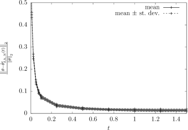
(a) ensemble size $N=5000$

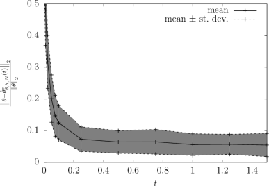
(b) ensemble size $N=100$

Figure 1. Mean and standard deviation of the estimator’s relative error for (35) with (36) as functions of $t$, with $h=\delta=10^{-3}$, and $\varepsilon=10^{-1}$, for two different ensemble sizes $N$.

To focus solely on the influence of the input perturbations, i.e. to verify the $\varepsilon$-stability of the methodology numerically, we plot the relative error in Figure 1(a) for a large ensemble size $N=5000$, so that all other error contributions are negligible. Specifically, we show the empirical mean and standard deviation of estimator’s relative errors, obtained by repeating the numerical experiment $100$ times. For very small values of $t$, one observes large relative errors indicating that the estimators, based on these approximations, are distorted. In view of (31) this is due to a large constant dominating the error. Increasing $t$, however, reduces the relative error significantly, i.e. the error constant shrinks. In fact, the mean relative error drops well below $5\%$ for $t\geq 0.2$ with only minor fluctuations, indicated by the small standard deviation. Roughly speaking, by increasing $t$ one increases the information content that is available to the estimator and the $\mathcal{O}(\varepsilon)$ contribution in error bound (31) becomes visible. As a matter of fact, the formal calculations in [Krumscheid2014_phd, Ch. 3.4] for a related estimator suggest that the multiscale error should even be $\mathcal{O}(\varepsilon^{2})$ for this toy example, which is also confirmed by the numerical experiments here. In fact, the estimator’s mean relative error is between $1\%$ and $2\%$ for $t\geq 0.75$, with standard deviations smaller than $6\cdot 10^{-3}$. To demonstrate the usefulness of bound (31), despite the fact that it is rather pessimistic, Figure 1(b) illustrates the mean and standard deviation of the estimator’s relative errors for the same experiment but with a smaller ensemble size $N$. By decreasing $N$, one can significantly reduce the computational cost while still controlling the relative error. Specifically, we use $N=100$ so that $1/\sqrt{N}=\mathcal{O}(\varepsilon)$, which in view of bound (31) should yield relative errors of the same order, with (possibly) larger fluctuations. As we have however seen in the previous experiment, the multiscale error is actually $\mathcal{O}(\varepsilon^{2})$ for this simple example, so that we now expect the estimator’s relative error to be dominated by the statistical error $1/\sqrt{N}=\mathcal{O}(\varepsilon)$. This is indeed confirmed in Figure 1(b). In fact, one finds qualitatively the same behaviour as before: the estimator is biased for small values of $t$, while increasing $t$ considerably reduces the mean relative error below $7\%$ with some fluctuations (standard deviation is smaller than $4\cdot 10^{-2}$).

Consider as a second example $h(x,y)=Ax+Bx^{3}$ and $\sigma(x)=\sqrt{\sigma_{a}+\sigma_{b}x^{2}}$, so that the coarse-grained system (35) associated with the multiscale system (34) reads

(37) $$dX=(AX+BX^{3})\,dt+\sqrt{2(\sigma_{a}+\sigma_{b}X^{2})}\,dW_{t}\;.$$

In this case, natural choices for the functions in (10) with $n=4$ parameters are

$$f_{1}(x) =x\;,\quad f_{2}(x)=x^{3}\;,\quad f_{3}(x)=0\;,\quad f_{4}(x)=0\;,$$

$$G_{1}(x) =0\;,\quad G_{2}(x)=0\;,\quad G_{3}(x)=2\;,\quad G_{4}(x)=2x^{2}\;,$$

where the true parameters are $\theta\equiv(\theta_{1},\theta_{2},\theta_{3},\theta_{4})^{T}=(A,B,\sigma_{a},\sigma_{b})^{T}$. As admissible function we select $\phi(x)=(1+x)\exp(-x^{2}/2)$ to meet the rank condition in Proposition 4.1, and we approximate the expectations by an ensemble average again. Finally, we consider $m=54$ trial points. Figure 2 depicts the

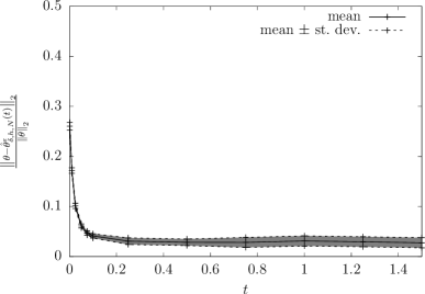
(a) ensemble size $N=5000$

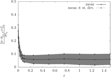
(b) ensemble size $N=100$

Figure 2. Mean and standard deviation of the estimator’s relative error for (37) as functions of $t$, with $h=\delta=10^{-3}$, and $\varepsilon=10^{-1}$, for two different ensemble sizes $N$.

mean and standard deviation of the estimated value’s relative error for the parameters in (37) corresponding to the choice $(A,B,\sigma_{a},\sigma_{b})=(3,-2,3/4,1/2)$ and $\varepsilon=0.1$ in (34). We consider again two different ensemble sizes $N\in\{100,5000\}$ and compute the empirical mean and standard deviations by repeating the same experiment $100$ times. Despite the fact that SDE (37), which models a meta-stable system for this parameter choices, provides a far more involved structure than the previous example, the estimation procedure shows qualitatively the same performance behaviour as before. For the large ensemble size $N=5000$, Figure 2(a) also displays that increasing $t$ reduces the mean relative error substantially (to about $3\%$) and only minor fluctuations (standard deviation is $10^{-2}$) are present. Even though the results for this example are slightly less accurate than the ones for the first example, also this example shows the validity of the error bound (31), although the bound also appears to be conservative for this example since actual multiscale error seems to be $\mathcal{O}(\varepsilon^{2})$ rather than $\mathcal{O}(\varepsilon)$. Furthermore, Figure 2(b) also demonstrates the practicality of bound (31) for this example: by decreasing the ensemble size to $N=100$, so that $1/\sqrt{N}=\mathcal{O}(\varepsilon)$, one observes mean relative errors that show qualitatively the same behaviour as a function of $t$ and that are of now dominated by the statistical error $1/\sqrt{N}=\mathcal{O}(\varepsilon)$, due to the fact that multiscale error is $\mathcal{O}(\varepsilon^{2})$ here. Moreover, the fluctuations are comparable to the ones observed in previous example (standard deviation is smaller than $4.5\cdot 10^{-2}$).

5.2. Brownian motion in a two-dimensional potential

Another example that falls into the class of multiscale diffusion processes is the movement model of Brownian motion in a two-scale potential. Specifically, consider the two-dimensional Langevin equation

$$dX^{\varepsilon}=-\nabla V\biggl{(}X^{\varepsilon},\frac{1}{\varepsilon}X^{\varepsilon};M\biggr{)}\,dt+\sqrt{2\sigma}\,dU_{t}\;,$$

where $V(\cdot,\cdot;M)$ denotes a two-scale potential with $M$ being a set of parameters controlling $V$ and $U$ denotes a standard two-dimensional Brownian motion used to model the thermal noise. We assume that the two-scale potential $V(\cdot,\cdot;M)$ is given by a large scale as well as a separable fluctuating part $V(x,y;M)=V(x;M)+p_{1}(y_{1})+p_{2}(y_{2})$, with $x,y\equiv(y_{1},y_{2})^{T}\in\mathbb{R}^{2}$, so that the original system reads

(38) $$dX^{\varepsilon}=-\Biggl{(}\nabla V(X^{\varepsilon};M)+\frac{1}{\varepsilon}\begin{pmatrix}p_{1}^{\prime}\bigl{(}X_{1}^{\varepsilon}/\varepsilon\bigr{)}\\ p_{2}^{\prime}\bigl{(}X_{2}^{\varepsilon}/\varepsilon\bigr{)}\end{pmatrix}\Biggr{)}\,dt+\sqrt{2\sigma}\,dU_{t}\;,$$

where $X^{\varepsilon}(t)\equiv{\bigl{(}X_{1}^{\varepsilon}(t),X_{2}^{\varepsilon}(t)\bigr{)}}^{T}\in\mathbb{R}^{2}$. Here we take the large scale part to be a quadratic potential $V(x;M)=\tfrac{1}{2}x^{T}Mx$, with $M\in\mathbb{R}^{2\times 2}$ being symmetric and positive definite, so that the coarse-grained equation for $X(t)\in\mathbb{R}^{2}$ is given by

(39) $$dX=-RMX\,dt+\sqrt{2\sigma R}\,dW_{t}\;,$$

with analytic expressions for $R=\operatorname*{diag}(r_{1},r_{2})$ [Pavliotis2007]. For the choices $p_{1}(y_{1})=\cos(y_{1})$ and $p_{2}(y_{2})=\cos(y_{2})/2$ we find that $r_{1}=I_{0}(1/\sigma)^{-2}$ and $r_{2}=I_{0}(1/(2\sigma))^{-2}$, where $I_{0}(z)$ denotes the modified Bessel function of the first kind. For this example a simple choice for the functions defining the parametrization (10) is

$$f_{1}(x)=\begin{pmatrix}x_{1}\\ 0\end{pmatrix}\;,\quad f_{2}(x)=\begin{pmatrix}x_{2}\\ 0\end{pmatrix}\;,\quad f_{3}(x)=\begin{pmatrix}0\\ x_{1}\end{pmatrix}\;,\quad f_{4}(x)=\begin{pmatrix}0\\ x_{2}\end{pmatrix}\;,$$

and $f_{5}(x)=f_{6}(x)=0$, as well as $G_{1}(x)=G_{2}(x)=G_{3}(x)=G_{4}(x)=0$ and

$$G_{5}(x)=\begin{pmatrix}2&0\\ 0&0\end{pmatrix}\;,\quad G_{6}(x)=\begin{pmatrix}0&0\\ 0&2\end{pmatrix}\;,$$

where $x\equiv{(x_{1},x_{2})}^{T}\in\mathbb{R}^{2}$. Hence, we seek to determine $n=6$ parameters, where the true parameters $\theta\equiv(\theta_{1},\dots,\theta_{6})^{T}$ are such that $\bigl{(}\begin{smallmatrix}\theta_{1}&\theta_{2}\\ \theta_{3}&\theta_{4}\end{smallmatrix}\bigr{)}=-RM$ and $\operatorname*{diag}(\theta_{5},\theta_{6})=\sigma R$. As admissible function we select here $\phi(x)=\Phi(x_{1})\Phi(x_{2})$, with $\Phi(z)=(1+z^{2})\exp(-z^{2}/2)$. Moreover, we choose $m=24$ trial points and approximate the expectations by ensemble averages ($N=5000$). Figure 3 shows the relative error of the

Figure 3. Relative error of the estimators $\hat{\theta}_{\delta,h,N}^{\varepsilon}$ for (39) as functions of $t$, with ensemble size $N=5000$, $h=\delta=10^{-3}$, and $\varepsilon=10^{-1}$.

estimated value as a function of $t$ based on observations of the multiscale system (38) with $M=\bigl{(}\begin{smallmatrix}2&2\\ 2&3\end{smallmatrix}\bigr{)}$, $\sigma=3/2$, and $\varepsilon=0.1$. Also here we observe that the relative error is significantly reduced to around $5\%$ by increasing $t$ and only minor fluctuations are present.

5.3. Brownian motion in a two-scale potential revisited

In the previous examples we always used an ensemble average to approximate the expectations. Here we illustrate that the proposed methodology can also be applied to the situation where only one long trajectory of observations (i.e. a time series) is available. Consider the one-dimensional Langevin equation

$$dX^{\varepsilon}=-\frac{d}{dx}V_{\alpha}\Bigl{(}X^{\varepsilon},\frac{1}{\varepsilon}X^{\varepsilon}\Bigr{)}\,dt+\sqrt{2\sigma}\,dU_{t}\;.$$

Let the two-scale potential $V_{\alpha}$ be given by a quadratic large scale part plus a fluctuating part, $V_{\alpha}(x,y)=\alpha x^{2}/2+p(y)$, so that the Langevin equation can be written as

(40) $$dX^{\varepsilon}=-\Bigl{(}\alpha X^{\varepsilon}+\frac{1}{\varepsilon}p^{\prime}\bigl{(}X^{\varepsilon}/\varepsilon\bigr{)}\Bigr{)}\,dt+\sqrt{2\sigma}\,dU_{t}\;.$$

When the fluctuating part $p$ is sufficiently smooth, bounded, and periodic with period $L$, the coarse-grained equation is given by

(41) $$dX=-AX\,dt+\sqrt{2\Sigma}\,dW_{t}\;,$$

with $A=\alpha L^{2}/(Z_{+}Z_{-})$ and $\Sigma=\sigma L^{2}/(Z_{+}Z_{-})$, where $Z_{\pm}=\int_{0}^{L}e^{\pm p(y)/\sigma}\,dy$.

To effectively use the estimation procedure based on one long trajectory of time discrete approximations of (40), the time discrete approximations have to satisfy a mixing condition, as detailed in Proposition 3.2. To check this condition, we assume that the time discrete approximations are the result of an Euler–Maruyama approximation and that $p^{\prime}$ is bounded. Let $g_{h}^{\varepsilon}(x):=(1-\alpha h)x-p^{\prime}(x/\varepsilon)h/\varepsilon$, then the Euler–Maruyama scheme applied to (40) on $[0,t=n_{t}h]$ can be written as

(42) $$\bar{X}_{h|\xi}^{\varepsilon}\bigl{(}(k+1)h\bigr{)}=g_{h}^{\varepsilon}\bigl{(}\bar{X}_{h|\xi}^{\varepsilon}(kh)\bigr{)}+\eta_{k}\sqrt{2\sigma h}\;,\quad\bar{X}_{h|\xi}^{\varepsilon}(0)=\xi\;,$$

for $0\leq k<n_{t}$, where the sequence of random variables ${(\eta_{k})}_{0\leq k<n_{t}}$ is i.i.d. with $\eta_{0}\sim\mathcal{N}(0,1)$. For any $h,\varepsilon>0$ sufficiently small, one can thus find $b,c>0$ and $a\in(0,1)$ such that $\left|g(x)\right|\leq a\left|x\right|-b$ for $\left|x\right|\geq c$, since $p^{\prime}$ is bounded. As the Euler–Maruyama scheme (42) generates essentially a stochastic difference equation of autoregressive type, it follows from [Doukhan1994, p. $102$] that the process ${\bigl{(}\bar{X}_{h|\xi}^{\varepsilon}(kh)\bigr{)}}_{k\geq 0}$ is strictly stationary and geometrically $\alpha$-mixing. Consequently, Proposition 3.2 ensures that the error of approximating the expectation by the regression estimator (20) vanishes and that the main convergence result (Proposition 4.1) holds.

To estimate the $n=2$ parameters in (41), we use $f_{1}(x)=x$, $f_{2}(x)=0=G_{1}(x)$, and $G_{2}(x)=2$ in the parametrization (10). For the numerical experiment below we set $p(y)=\cos(y)$ so that the true parameters are $\theta\equiv(\theta_{1},\theta_{2})^{T}={I_{0}(\sigma^{-1})}^{-2}(-\alpha,\sigma)^{T}$, with $I_{0}(z)$ again denoting the modified Bessel function of first kind. Moreover, we use $m=24$ trial point and $\phi(x)=\exp(-x^{2}/2)$ as admissible function.

Figure 4. Relative error of the estimators $\hat{\theta}_{\delta,h,N}^{\varepsilon}$ for (41) as functions of $t$, using $h=\delta=10^{-3}$, $\varepsilon=10^{-1}$, and a single time series on $[0,5000]$.

Figure 4 shows the relative error of the estimated value as a function of $t$, when one trajectory of observations on $[0,5000]$ is obtained from the multiscale system with $(\alpha,\sigma)=(2,1)$, and $\varepsilon=0.1$. The same behaviour of the relative error as a function of $t$ is evident: very small $t$ yields distorted estimated values, while increasing $t$ reduces the error significantly. In fact, for $t\geq 0.1$ the relative error drops well below $5\%$ with only minor fluctuations. Since bound (31) is not guaranteed to be valid in this case, the constants in front of the rates might depends on other parameters (see discussion in Section 4.3). Therefore we chose a rather long time series to focus solely on $\varepsilon$-stability, that is on the influence of the perturbation of the input, and to illustrate the convergent behaviour of the estimation procedure.

6. Conclusion

We have studied the convergence of parametric estimation procedures for diffusion processes from a numerical analysis perspective. Specifically, we have introduced consistency, stability, and convergence concepts for estimation procedures. It turns out that the maximum likelihood estimator is not convergent within this framework, since it fails to be stable. Conversely, we have introduced an inference methodology which is provably convergent within this framework. This convergence property of an estimation procedure is pivotal in many applications, such as for data-driven coarse-graining approaches from multiscale observations. We have studied several examples of this class to verify the theoretical results of the introduced methodology. Furthermore, these examples demonstrate that the estimation procedure can be used to accurately approximate parameters in both the drift function and the diffusion function.

There are still many challenges that remain to be addressed. One is, for example related to the rigorous verification of the mixing conditions in the case where only one time series is available. From a theoretical perspective this is not easy, as the available theory is quite restrictive. In fact, most of it is only applicable for a constant diffusion coefficient and a drift satisfying a linear growth condition; see, e.g., [Klokov2013] and references therein. Standard conditions on drift and diffusion functions ensuring the mixing conditions of the continuous time diffusion process are, e.g., given in [Veretennikov1987, Veretennikov1989, Leblanc1997]. From a practical perspective, however, this condition does not appear to be too restrictive, as the results in [Kalliadasis2015] indicate.

But there are also other interesting questions left open. During the construction of the estimator, for example, there are still some degrees of freedom, which we have not used optimally yet. For instance, it seems that the particular choice of the admissible function $\phi$ can influence the error constant of the error bound. Therefore, an important task for future research is to study whether or not one can minimise the error constant not only with respect to $\phi$, but also with respect to the number and location of the trial points. Moreover, characterising the error constant’s dependency on the parameter $t$ is also desirable. A closely related avenue for future efforts is also the study of the asymptotic distribution of the estimators, which in turn can be used to guide the construction of asymptotic confidence intervals for the estimated values. These and related topics will be treated in future studies.