Dynamic message-passing approach for kinetic spin models with reversible dynamics

Abstract

A method to approximately close the dynamic cavity equations for synchronous reversible dynamics on a locally tree-like topology is presented. The method builds on (a) a graph expansion to eliminate loops from the normalizations of each step in the dynamics, and (b) an assumption that a set of auxilary probability distributions on histories of pairs of spins mainly have dependencies that are local in time. The closure is then effectuated by projecting these probability distributions on $n$-step Markov processes. The method is shown in detail on the level of ordinary Markov processes ($n=1$), and outlined for higher-order approximations ($n>1$). Numerical validations of the technique are provided for the reconstruction of the transient and equilibrium dynamics of the kinetic Ising model on a random graph with arbitrary connectivity symmetry.

I Introduction

Disordered spin systems are an important class of models able to catch and reproduce a large range of phenomena from phase transitions in magnets and amorphous systems crisanti2007amorphous to protein folding in biology goldstein1992optimal , social media facchetti2011computing ; kirkpatrick2012social , epidemic spreading pastor2001epidemic , immune and neural networks amit1992modeling , applications in finance and optimisation problems coolen2005mathematical ; mezard2002analytic ; PhysRevLett.87.127209 . In the thermodynamic limit these systems have rich and fascinating repertoires of static and dynamic behaviour including the clustering mezard2002analytic or shattering achlioptas2010algorithmic transition, ergodicity breaking and ageing bouchaud1997out . To systematically describe their static properties the replica method (for fully connected systems) and the cavity method (for dilute systems) were developed mezard2009information . General techniques to systematically study the dynamics of single finite systems in this class have however been less developed and in practice mostly limited to dynamic mean-field theories Kappen98 ; kappen2000mean , path integral techniques de1978dynamics ; Sompolinsky1982 ; sommers1987path ; RoudiHertz11JSAT , large deviation approaches del2014perturbative and, above all, numerical simulation Gillespie77 .

The cavity method mezard2009information ; yedidia2003understanding here holds a special place as it has become the method of choice to solve the statics of models on sparse networks, while for dynamics it was long restricted to dynamics on fully asymmetric graphs derrida1987exactly ; Mezard11 ; aurell2011three . The main problem is that while the cavity technique reduces the complexity “in space” (number of terms in an approximate computation of marginals), there remains a complexity “in time” (cardinality of each term). This is so because the natural variables of the dynamic cavity method are probabilities of spin histories of which there are exponentially many ($2^{t}$ for synchronous updates over time $[0,t]$ with time constant one). Therefore, although the dynamic cavity equations themselves only involve a finite number of terms, summing them nevertheless (in general) entails a number of operations which is exponentially large in $t$. Fully asymmetric networks is a special case since the cavity equations can then be marginalized over time with no loss of information, and the complexity “in time” disappears. Alternative “ways out” investigated in the literature use additional assumptions on the evolution law such as majority dynamics Kanoria2011 (i.e. linear dynamics with thresholding) or, more recently, unidirectional dynamics. Models of this latter type, where after a variable makes a transition from a state to another it can never go back, are represented by the zero-temperature random field Ising model (RFIM) ohta2010universal , cascade processes altarelli2013large , spread optimization problems altarelli2013optimizing and several epidemic models as, for instance, the susceptible-infected-recovered (SIR) model lokhov2013inferring ; lokhov2014dynamic . The main peculiarity of such models is that the dynamics can be parametrized in terms of the time(s) at which the transition from one state of the variable to another occurs, which again eliminates time complexity.

Another approach was taken in Neri2009 , where a simplifying “one-time” assumption was introduced, which for fully asymmetric networks reduces to (exact) marginalization over time. For the kinetic Ising model with synchronous and asynchronous updates this was later shown to be considerably more accurate than dynamic mean-field, not only for asymmetric networks but also for partly symmetric networks aurell2011message ; aurell2012dynamic . A different approach, based on variational approximations, was very recently proposed in pelizzola2013variational where the author shows better performances in recovering stationary states compared to existing methods. Unfortunately, except for fully asymmetric networks all these approaches are limited to steady states, and hence cannot handle dynamic phenomena.

In this contribution we present a method to approximatively close the dynamic cavity equations for synchronous updates with no assumptions on the underlying network and evolution law beyond that the network is locally tree-like and the evolution law is Markov. Unlike other methods already present in the literature, our approach is built not only to recover stationary states but potentially also the transient, i.e. the out of equilibrium dynamics. The method is built on two ingredients. The first, which already appeared in this context in altarelli2013optimizing , is the use of the graph expansion technique of mezard2009information to rewrite the probabilistic model in a way such that the underlying graph is explicitly locally tree-like, and the standard cavity equations can be used. The second ingredient is the assumption that a set of auxilary probability distributions on spin histories, “messages” in cavity method language, contain dependenciess that are mainly local in time. A closure of the dynamic cavity equations is then effectuated within the class of $n$-order Markov processes. For definiteness we will here present the closure in the class of ordinary Markov processes ($n=1$) and only outline the extensions to $n>1$, to which we intend to return in a future contribution. The pioneering contribution Neri2009 can, in present perspective, be seen as a closure in the class of Bernoulli processes ($n=0$), without using graph expansion.

II The dynamic cavity equations

We consider a probabilistic graphical model defined on a tree-like graph $\mathcal{G}=(V,E)$ where $V$ is a set of $N$ vertices and $E$ is a set of directed edges. Spins, Boolean variables $\sigma_{i}(t)=\pm 1$, are associated to each vertex at each time. We denote by $X_{i}=(\sigma_{i}(0),\sigma_{i}(1),\dots,\sigma_{i}(t))$ the spin history of spin $i$ and the evolution law $w_{i}(\sigma_{i}^{s}|\sigma_{i}^{s-1},\{\sigma_{j}^{s-1}\}_{j\in\partial i})$ is the conditional probability of spin $i$ to take value $\sigma_{i}$ at time $s$ given the values of spins $i$ and $\partial i$, the graph neighbours of $i$, at time $s-1$. We note that this class is larger than the previously investigated majority dynamics and (synchronous) kinetic Ising models since we allow the evolution law to depend on $\sigma_{i}^{s-1}$. The joint probability over the spin histories can be then written as

$$P(X_{1},\dots,X_{N})=\prod_{i\in V}\prod_{s=1}^{t}w_{i}(\sigma_{i}^{s}|\sigma_{i}^{s-1},\{\sigma_{j}^{s-1}\}_{j\in\partial i})P_{0}$$ (1)

where $P_{0}=P(\sigma_{1}(0),\dots,\sigma_{N}(0))$ is the initial joint distribution at time zero and $t$ is the final time. We recall that the cavity method works well when the underlying network is (locally) tree-like. Being a conditional probability any evolution law $w_{i}$ can be written as $\exp\left(\sigma_{i}^{s}\Psi_{i}-\log 2\cosh\Psi_{i}\right)$ where $\Psi_{i}$ is some function of $(\sigma_{i}^{s-1},\{\sigma_{j}^{s-1}\})$. $w_{i}$ hence contains two types of “interactions”, namely $\sigma_{i}^{s}\Psi_{i}$ and $\log 2\cosh\Psi_{i}$, and if $P(X_{1},\dots,X_{N})$ in (1) is written as $\exp\left(F(X_{1},\dots,X_{N})\right)$ the graph describing the dependencies in $F$ will have short loops, which necessarly emerge even if the network topology is tree-like, as illustrated in Fig 1.

Figure 1: Color online. Original graph topologically tree-like shown in a factor graph representation in which loops emerge naturally in time when dynamics is considered. Circles illustrate spin variables and squares interactions among them. More specifically, black squares picture the interaction between one spin and one of its neighbours, i.e. $\phi_{ij}(\sigma_{i}(t),\sigma_{j}({t-1}))$, whereas coloured squares picture the interaction among neighbours of a given spin, i.e. $\phi_{j}(\{\sigma_{j}(t-1)\}_{j\in\partial i})$.

As shown in mezard2009information ; altarelli2013optimizing such loops can however be removed by defining an auxiliary factor graph at the price that the new variable nodes will contain more that one old variable. The procedure consists in changing the old variable nodes into factor nodes and changing the old interaction edges into new variable nodes. The resulting topology of the new expanded graph is shown in Fig. 2 where each variable node now contains the spin histories of two spins. The functions sitting on the new factor nodes are defined in order to guarantee all interactions to remain the same as in the original graph and so, for consistency, the spin variables of the same type that appear on different (new) variable nodes have to take the same value.

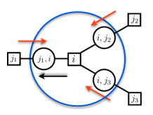
Figure 2: Auxiliary graph obtained from the original one shown in Fig. 1 where the time-loops have been removed with a standard procedure. The new variable nodes contain the spin history of two variables which were neighbours in the original graph and factor nodes contain the interactions needed to generate and pass this history, i.e. $\tilde{\Phi}=\delta_{X_{i}^{(ij_{1})},\dots,X_{i}}\prod_{s=1}^{t}w_{i}(\sigma_{i}^{s}|\sigma_{i}^{s-1},\{\sigma_{j}^{s-1}\}_{j\in\partial i})P_{0}(\sigma_{i},\{\sigma_{j}\}_{j\in\partial i})$. Observe that the delta function is already summed over in the main text.

In the auxiliary graph the node $(i,j)$ contains the pair $(X_{i}^{(ij)},X_{j}^{(ij)})$ where by $X_{i}^{(ij)}$ we mean a variable of the same kind as spin history $X_{i}$ residing in the node $(i,j)$. The joint probability distribution of the new variables on the expanded factor graph of Fig. 2 can then be written as:

$$P(\{X_{i}^{(ij)},X_{j}^{(ij)}\}_{(ij)\in E})= \prod_{i\in V}\delta_{X_{i}^{(ij_{1})},\,X_{i}^{(ij_{2})},\dots,X_{i}}\prod_{s=1}^{t}w_{i}(\sigma_{i}^{s}|\sigma_{i}^{s-1},\{\sigma_{j}^{s-1}\}_{j\in\partial i})P_{0}$$ (2)

where all the variables in $w_{i}(\sigma_{i}^{s}|\sigma_{i}^{s-1},\{\sigma_{j}^{s-1}\}_{j\in\partial i})$ are taken from the surrounding spin histories $(X_{i}^{(ij_{1})},X_{i}^{(ij_{2})},\dots)$ and the constraint enforces that these histories agree. If the original graph is (locally) tree like, this procedure removes the loops in time and gives us a new auxiliary graph which is also (locally) tree like. The standard belief propagation (BP) update equations can then be written, for the variables in the new graph, as in the static case (see eq. (14.15) in mezard2009information ) as:

$$m_{i\to(ij)}(X_{i},X_{j})\propto \sum_{\{X_{k}\}}\Phi(X_{i},X_{j},\{X_{k}\})\prod_{k\in\partial i\backslash j}m_{k\to(ik)}(X_{k},X_{i})$$ (3)

where $\Phi(X_{i},X_{j},\{X_{k}\})=P_{0}\prod_{s=1}^{t}w_{i}(\sigma_{i}^{s}|\sigma_{i}^{s-1},\{\sigma_{k}^{s-1}\}_{k\in\partial i\backslash j},\sigma_{j}^{s-1})$ is analogous to a potential sitting in the factor nodes which transfers the dynamics to its neighbour variable nodes and the normalization factor can be computed by the condition that $\sum_{X_{i},X_{j}}m_{i\to(ij)}(X_{i},X_{j})=1$. Above we have shortened the notation to $X_{i}=X_{i}^{(ij)}$, $X_{k}=X_{k}^{(ik)}$ and the same for $X_{j}$ and all the $\sigma$-variables contained in $w_{i}$. Let us note that we have fewer distinct messages respect to the static BP formulation since messages from factor to variable nodes are, in this case, the same as messages from variable to factor nodes, i.e. $m_{j\to(ij)}(X_{j},X_{i})=m_{(ij)\to i}(X_{j},X_{i})$. Hence, for the topology shown in Fig 2, the message on the LHS of (3) is illustrated in black whereas the messages on the RHS are those two in red coming from the right side of the picture. To simplify notation, from now on variables with no apex refer to variables at time $t$, i.e. $\sigma_{i}=\sigma_{i}(t)$, whereas variables with apex(es) refer respectively to previous time(s), i.e. $\sigma_{i}^{\prime}=\sigma_{i}(t-1),\sigma_{i}^{\prime\prime}=\sigma_{i}(t-2),\dots$ and so $X_{i}^{{}^{\prime}}$ is the spin history of spin $i$ up to time $t-1$. Let us observe that, while notationally compact, equations (3) is, except for short times, computationally intractable as the right-hand side involves sums over complete spin histories.

III Markovian closure of the dynamic cavity equations

We first observe that, given the Markovianity of the dynamics contained in $\Phi(X_{i},X_{j},\{X_{k}\})$, the messages $m_{i\to(ij)}(X_{i},X_{j})$ in (3) actually do not depend on the spin variable $\sigma_{j}$ at time $t$ but only at time $t-1$ and earlier times. The messages $m_{i\to(ij)}(X_{i},X_{j})$ are hence always uniform distributions on $\sigma_{j}(t)$ and, since $\sigma_{j}(t)$ is therefore a kind of dummy argument, we may simplify the notation by writing $m_{i\to(ij)}(X_{i},X_{j}^{{}^{\prime}})$. Furthermore, if we use the same simplification on the right hand side of (3) we have incoming messages $m_{k\to(ik)}(X_{k},X_{i}^{{}^{\prime}})$ which can be marginalized to $m_{k\to(ik)}(X_{k}^{{}^{\prime}},X_{i}^{{}^{\prime}})$ as there is no other dependence on $\sigma_{k}$, the value of spin $k$ at time $t$. Using Markovianity again we can simplify further to $m_{k\to(ik)}(X_{k}^{{}^{\prime}},X_{i}^{{}^{\prime\prime}})$ and write (3) as

$$m_{i\to(ij)}(X_{i},X_{j}^{{}^{\prime}})\propto \sum_{\{X_{k}^{{}^{\prime}}\}}\Phi(X_{i},X_{j}^{{}^{\prime}},\{X_{k}^{{}^{\prime}}\})\prod_{k\in\partial i\backslash j}m_{k\to(ik)}(X_{k}^{{}^{\prime}},X_{i}^{{}^{\prime\prime}})$$ (4)

Equation (4) shows that the dynamic cavity equations have a different structure and are actually, in some respects, simpler than standard BP updates, since if all messages up to some time $t-1$ are known, messages up to time $t$ can be evaluated directly without the need to iterate to a fixed point.

III.1 Fully asymmetric graph

It is worth to observe how equation (4) simplifies when referred to a fully asymmetric graph, with interaction couplings between node $i$ and $j$ such that $J_{ij}\neq 0$ and $J_{ji}=0$. Under this assumption the interaction function $\Phi$ no longer depends on the spin history $X_{j}^{{}^{\prime}}$ and, as a consequence, the message on the LHS of the equation does not depend on that history either, since such dependence is carried in only through the function $\Phi$. For consistency, we can apply the same argument to the messages on the RHS and conclude that they only depend on the spin history $X_{k}^{{}^{\prime}}$ and no longer on $X_{i}{{}^{\prime\prime}}$. Then remembering that $\Phi$ is a normalized function respect to the variable $\sigma_{i}^{s}$, as shown in the text below equation (3), we can sum both sides of (4) over the spin history $X_{i}^{{}^{\prime}}$ and then make use of the sum over $\{X_{k}^{{}^{\prime}}\}$ on the RHS to obtain the simplified version of the dynamic message-passing equation for fully asymmetric graph

$$m_{i\to(ij)}(\sigma_{i}^{t})= \sum_{\{\sigma_{k}^{t-1}\}_{k\in\partial i\backslash j}}w_{i}(\sigma_{i}^{t}|\{\sigma_{k}^{t-1}\}_{k\in\partial i\backslash j})\prod_{k\in\partial i\backslash j}m_{k\to(ik)}(\sigma_{k}^{t-1}).$$ (5)

This equation is agreement with previous literature for the same graph topology Neri2009 ; aurell2011message ; aurell2011three .

III.2 Graph with arbitrary connectivity symmetry

In what follows we propose a Markovian closure of the dynamic BP update equation (4) for a network with arbitrary connectivity symmetry. In the next section the same closure is used to derivate the dynamic BP output equations. In a closure in the class of $n$-th order Markov processes we assume $m_{i\to(ij)}(X_{i},X_{j}^{{}^{\prime}})=\prod_{s=n}^{t}T^{(n)}_{i\to(ij)}(\sigma_{i}^{s}|\sigma_{i}^{s-1},\sigma_{j}^{s-1},\ldots,\sigma_{i}^{s-n},\sigma_{j}^{s-n})$ and solve (4) iteratively. We here consider $n=1$. The marginalizations over the last and last two times of the variable node $(i,j)$ are

$$P_{i\to(ij)}^{(t-1)}(\sigma_{i}^{{}^{\prime}},\sigma_{j}^{{}^{\prime}}) =\sum_{\begin{subarray}{c}X_{i}^{{}^{\prime\prime}},X_{j}^{{}^{\prime\prime}}\end{subarray}}m_{i\to(ij)}(X_{i}^{{}^{\prime}},X_{j}^{{}^{\prime\prime}})$$ (6)

$$P_{i\to(ij)}^{(t,\,t-1)}(\sigma_{i},\sigma_{i}^{{}^{\prime}},\sigma_{j}^{{}^{\prime}}) =\sum_{X_{i}^{{}^{\prime\prime}},\,X_{j}^{{}^{\prime\prime}}}m_{i\to(ij)}(X_{i},X_{j}^{{}^{\prime}}),$$ (7)

by assumption linked by

$$P^{(t,\,t-1)}(\sigma_{i},\sigma_{i}^{{}^{\prime}},\sigma_{j}^{{}^{\prime}})=T(\sigma_{i}|\sigma_{i}^{{}^{\prime}},\sigma_{j}^{{}^{\prime}})\,P^{(t-1)}(\sigma_{i}^{{}^{\prime}},\sigma_{j}^{{}^{\prime}})$$ (8)

where we omitted the subscript $i\to(ij)$ and the superscript time dependence of $T^{(t,t-1)}$ for readability. We note that by above $P^{(t-1)}(\sigma_{i}^{{}^{\prime}},\sigma_{j}^{{}^{\prime}})$ actually does not depend on its second argument and we will therefore from now on simplify to $P^{(t-1)}(\sigma_{i}^{{}^{\prime}})$. Closure means to make the same assumptions for the upstream messages $m_{k\to(ik)}(X_{k},X_{i}^{{}^{\prime}})$, use (4) to compute $P_{i\to(ij)}^{(t-1)}$ and $P_{i\to(ij)}^{(t,\,t-1)}$ in (6) and (7), and then take (8) to define $T(\sigma_{i}|\sigma_{i}^{{}^{\prime}},\sigma_{j}^{{}^{\prime}})$. This can be done by introducing an auxiliary function $\mathcal{F}$

$$\mathcal{F}_{i\to(ij)}^{(t-1)}(\sigma_{i}^{{}^{\prime}},\{\sigma_{k}^{{}^{\prime}}\}_{k\in\partial i\backslash j}) =\sum_{\begin{subarray}{c}\{X_{k}^{{}^{\prime\prime}},\,X_{i}^{{}^{\prime\prime}},\,X_{j}^{{}^{\prime\prime}}\}\end{subarray}}\prod_{k\in\partial i\backslash j}\,m_{k\to(ik)}(X_{k}^{{}^{\prime}},X_{i}^{{}^{\prime\prime}})\prod_{s=1}^{t-1}w_{i}(\sigma_{i}^{s}|\sigma_{i}^{s-1},\{\sigma_{k}^{s-1}\}_{k\in\partial i\backslash j},\sigma_{j}^{s-1})P_{0}$$ (9)

which is strictly a specific marginalization of the right hand side of (4). From now on, we use the notation $\{\sigma_{k}\}_{\backslash}=\{\sigma_{k}\}_{k\in\partial i\backslash j}$ and $\prod_{k\backslash}=\prod_{k\in\partial i\backslash j}$. In terms of (9) we have

$$P_{i\to(ij)}^{(t-1)}(\sigma_{i}^{{}^{\prime}}) \propto\sum_{\{\sigma_{k}^{{}^{\prime}}\}}\mathcal{F}_{i\to(ij)}^{(t-1)}(\sigma_{i}^{{}^{\prime}},\{\sigma_{k}^{{}^{\prime}}\}_{\backslash})$$ (10)

$$P_{i\to(ij)}^{(t,\,t-1)}(\sigma_{i},\sigma_{i}^{{}^{\prime}},\sigma_{j}^{{}^{\prime}}) \propto\sum_{\{\sigma_{k}^{{}^{\prime}}\}}\,w_{i}(\sigma_{i}|\sigma_{i}^{{}^{\prime}},\{\sigma_{k}^{{}^{\prime}}\}_{\backslash},\sigma_{j}^{{}^{\prime}})\,\mathcal{F}_{i\to(ij)}^{(t-1)}(\sigma_{i}^{{}^{\prime}},\{\sigma_{k}^{{}^{\prime}}\}_{\backslash})$$ (11)

On the other hand, by the (assumed) Markovianity of the upstream messages we can write an iterative equation in time for $\mathcal{F}$:

$$\mathcal{F}_{i\to(ij)}^{(t)}(\sigma_{i},\{\sigma_{k}\}_{\backslash}) =\sum_{\{\sigma_{k}^{{}^{\prime}}\},\sigma_{i}^{{}^{\prime}},\sigma_{j}^{{}^{\prime}}}\prod_{k\backslash}T_{k\to(ik)}(\sigma_{k}|\sigma_{k}^{{}^{\prime}},\sigma_{i}^{{}^{\prime}})\,w_{i}(\sigma_{i}|\sigma_{i}^{{}^{\prime}},\{\sigma_{k}^{{}^{\prime}}\}_{\backslash},\sigma_{j}^{{}^{\prime}})\,\mathcal{F}_{i\to(ij)}^{(t-1)}(\sigma_{i}^{{}^{\prime}},\{\sigma_{k}^{{}^{\prime}}\}_{\backslash}).$$ (12)

Whereas the iterative equation for $T$, using (10) and (11), reads as

$$T_{i\to(ij)}(\sigma_{i}|\sigma_{i}^{{}^{\prime}},\sigma_{j}^{{}^{\prime}})=\frac{\sum_{\{\sigma_{k}^{{}^{\prime}}\}}w_{i}(\sigma_{i}|\sigma_{i}^{{}^{\prime}},\{\sigma_{k}^{{}^{\prime}}\}_{\backslash},\sigma_{j}^{{}^{\prime}})\,\mathcal{F}_{i\to(ij)}^{(t-1)}(\sigma_{i}^{{}^{\prime}},\{\sigma_{k}^{{}^{\prime}}\}_{\backslash})}{\sum_{\sigma_{i},\,\{\sigma_{k}^{{}^{\prime}}\}}w_{i}(\sigma_{i}|\sigma_{i}^{{}^{\prime}},\{\sigma_{k}^{{}^{\prime}}\}_{\backslash},\sigma_{j}^{{}^{\prime}})\,\mathcal{F}_{i\to(ij)}^{(t-1)}(\sigma_{i}^{{}^{\prime}},\{\sigma_{k}^{{}^{\prime}}\}_{\backslash})},$$ (13)

where the denominator takes care of the normalization. Equation (12) and (13), which solve the dynamic cavity equations under the assumption that messages are Markovian, are the first result of this paper and represent the ingredients to solve the BP update equations at any time. The entire procedure clearly takes polynomial time instead of an exponential time as the original formulation and, as noted above, does not involve iteration to fixed point.

IV Markovian closure of the BP output equations

We now turn to the BP output equations, i.e. the equations for the actual marginal probability both on the auxiliary and on the original factor graph. The marginal probability of one variable node $(i,j)$ in the auxiliary graph is simply given by the product of the incoming messages to the node $(i,j)$:

$$P_{(ij)}(X_{i},X_{j})\propto m_{i\to(ij)}(X_{i},X_{j}^{{}^{\prime}})\,m_{j\to(ij)}(X_{j},X_{i}^{{}^{\prime}}).$$ (14)

We are however interested in the single-site one-time marginal probability on the original graph, $P_{i}(\sigma_{i}(t))$, from which we can compute physical observables of interest such as, for instance, the magnetization at any given time. We can get this marginal starting from the one-site marginal probability on a spin history, $P_{i}(X_{i})$. In terms of the auxiliary probability distribution on the expanded graph this reads as

$$P_{i}(X_{i}) \propto\sum_{X_{j}}\prod_{j\in\partial i}m_{j\to(ij)}(X_{j},X_{i}^{{}^{\prime}})\Big{[}\prod_{s=1}^{t}w_{i}(\sigma_{i}^{s}|\sigma_{i}^{s-1},\{\sigma_{j}^{s-1}\}_{j\in\partial i})P_{0}\Big{]},$$ (15)

where spins $j$’s are the neighbours of site $i$ in the original and expanded graph (see Fig 2). To solve these equations on the same level of approximation as the update equation we define a new auxiliary function

$$\mathcal{G}^{(t-1)}(\sigma_{i}^{{}^{\prime}},\{\sigma_{j}^{{}^{\prime}}\}_{j\in\partial i})= \sum_{X_{i,}^{{}^{\prime\prime}}\{X_{j}^{{}^{\prime\prime}}\}_{j\in\partial i}}\prod_{j\in\partial i}m_{j\to(ij)}(X_{j}^{{}^{\prime}},X_{i}^{{}^{\prime\prime}})\Big{[}\prod_{s=1}^{t-1}w_{i}(\sigma_{i}^{s}|\sigma_{i}^{s-1},\{\sigma_{j}^{s-1}\}_{j\in\partial i})P_{0}\Big{]}.$$ (16)

The single-site one-time and two-time marginal probabilities on the original graph then follow from (15):

$$P^{(t-1)}_{i}(\sigma_{i}^{{}^{\prime}}) \propto\sum_{\{\sigma_{j}^{{}^{\prime}}\}_{j\in\partial i}}\mathcal{G}^{(t-1)}(\sigma_{i}^{{}^{\prime}},\{\sigma_{j}^{{}^{\prime}}\}_{j\in\partial i}),$$ (17)

$$P^{(t,\,t-1)}_{i}(\sigma_{i},\sigma_{i}^{{}^{\prime}}) \propto\sum_{\{\sigma_{j}^{{}^{\prime}}\}_{j\in\partial i}}w_{i}(\sigma_{i}|\sigma_{i}^{{}^{\prime}},\{\sigma_{j}^{{}^{\prime}}\}_{j\in\partial i})\,\mathcal{G}^{(t-1)}(\sigma_{i}^{{}^{\prime}},\{\sigma_{j}^{{}^{\prime}}\}_{j\in\partial i}).$$ (18)

In analogy to $\mathcal{F}$ above, we can write a recursive equation for $\mathcal{G}$ by using the Markovian assumption for messages:

$$\mathcal{G}^{(t)}(\sigma_{i},\{\sigma_{j}\}_{j\in\partial i}) =\sum_{\sigma_{i}^{{}^{\prime}},\{\sigma_{j}^{{}^{\prime}}\}_{j\in\partial i}}\prod_{j\in\partial i}T_{j\to(ij)}(\sigma_{j}|\sigma_{j}^{{}^{\prime}},\sigma_{i}^{{}^{\prime}})\,w_{i}(\sigma_{i}|\sigma_{i}^{{}^{\prime}},\{\sigma_{j}^{{}^{\prime}}\}_{j\in\partial i})\,\mathcal{G}^{(t-1)}(\sigma_{i}^{{}^{\prime}},\{\sigma_{j}^{{}^{\prime}}\}_{j\in\partial i})$$ (19)

Hence starting with initial value for the functions $T$, $\mathcal{F}$ and $\mathcal{G}$ equations (12), (13) and (19) can be iterated up to the desired time and equation (17) can be used to compute the time-dependent marginal probability of site $i$. We highlight that unlike the original formulation, which takes an exponential time to compute marginals, the entire scheme presented here has a polynomial computational cost.

V Results

In this section we test the accuracy of our dynamic message-passing (DMP) approach on a statistical physics model often chosen as a case of study to investigate dynamics of complex systems: the kinetic Ising model.

V.1 A case of study: the kinetic Ising model with arbitrary connectivity symmetry

We compare the performance of DMP to Monte Carlo Markov Chain simulations (MC) with Glauber dynamics on the kinetic Ising model on a random diluted graph with arbitrary connectivity symmetry: fully symmetric, partially asymmetric and fully asymmetric network. The comparison is performed computing the behaviour of the magnetization of the model both during the transient and at equilibrium (or at the stationary states when detailed balance does not hold). Following hatchett2004parallel we introduce a connectivity matrix $c_{ij}$ where $c_{ij}=1$ if there is a link from vertex $i$ to vertex $j$, $c_{ij}$ = 0 otherwise, and matrix elements $c_{ij}$ and $c_{kl}$ are independent unless $\{kl\}=\{ji\}$. The following distributions then specify the graph topology: the marginal one-link distribution

$$p(c_{ij})=\frac{c}{N}\delta_{1,c_{ij}}+(1-\frac{c}{N})\delta_{0,c_{ij}}$$ (20)

and the conditional distribution

$$p(c_{ij}|c_{ji})=\epsilon\delta_{c_{ij},c_{ji}}+(1-\epsilon)p(c_{ij}).$$ (21)

Above, $N$ is the size of the network, $c$ the average connectivity and $\epsilon\in[0,1]$ a parameter which controls the asymmetry. The value $\epsilon=0$ gives a fully asymmetric network whereas $\epsilon=1$ a fully symmetric one.

In the kinetic Ising model the transition probability rate $w_{i}$, which appears above, is given by $w_{i}(\sigma_{i}^{s}|\{\sigma_{j}^{s-1}\})=\exp{(\beta\sigma_{i}^{s}J_{ij}\sigma_{j}^{s-1}-\log 2\cosh(\beta\sum_{j}J_{ij}\,\sigma_{j}^{s-1}}))$ where the $j$’s variable are neighbours of spin $i$, $J_{ij}$ are the interaction strengths between site $i$ and $j$ and $\beta$ is the inverse temperature. We observe that this model belongs to a subclass of the models considered within the general formulation above as the transition rate does not depend explicitly on $\sigma_{i}^{s-1}$. Since we here want to mainly investigate the effect of the asymmetry on the performances of our algorithm, we restrict our numerical analysis to ferromagnetic models, i.e. interaction strength $J_{ij}=J>0$ for every pair of sites $i,j$. For simplicity, all the spins on the graph are chosen independent at the initial time although correlated initial conditions could also be considered in the above formulation. Results are shown in Figure 3 for several values of the initial magnetization at different temperatures and for various values of the asymmetry parameter $\epsilon$.

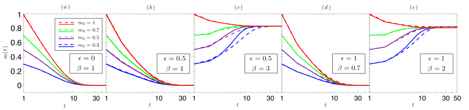
Figure 3: Color online. Comparison between dynamic message passing algorithm (solid lines) and Monte Carlo simulation (dashed lines) for the evolution of the magnetization $m(t)$ in an Erdös Rényi network of $N=5000$ nodes and average connectivity $c=3$. Different colors represent different initial magnetizations $m(0)$, from the largest (upper line) to the smallest (lower line) according to the legend. (b) and (c) plot: partially asymmetric network ($\epsilon=0.5$) respectively at low and high temperatures. (d) and (e) plot: fully symmetric network respectively at low and high temperatures. In MC simulations $m(t)$ is averaged over 5000 samples.

Numerical results for fully asymmetric networks are obtained by using the simplified version (5) of the dynamic message-passing equation and, as expected from Neri2009 ; aurell2011message ; aurell2012dynamic , they show a perfect agreement with Monte Carlo simulations both for the computation of the transient and the stationary state (see panel $(a)$). When the full asymmetry is broken and a network with feedback is considered numerics is obtained through the DMP scheme presented above. Comparison with MC shows that the results provided by DMP are still very good for high enough temperature (above the critical transition) both for partially and fully symmetric connectivities. Indeed as it is possible to note from Fig 3 (partially asymmetric network in panel $(b)$ and fully symmetric one in panel $(d)$) the transient regime is very well reproduced by DMP and the stationary (or equilibrium) state is the same as MC. When temperature is decreased below the critical ferromagnetic transition the performances of DMP start getting worse (panel $(c)$ and $(e)$). In this regime, the transient is very well recovered only for the first few initial steps of the dynamics and gets progressively worse for longer times. Nevertheless, for the partially asymmetric network considered $(\epsilon=0.5)$ the stationary state reached by DMP and MC simulations coincide, although DMP has a faster convergence to that (panel $(c)$). For fully symmetric networks similar considerations follow for the transient regime although the equilibrium state reached by DMP and MC simulations at this temperature are slightly different (panel $(e)$). This is not always the case indeed we noticed numerically that, for some of the temperatures even below the critical transition, DMP reaches the same equilibrium state as MC (see for instance Fig 4, panel (c)). However, for fully symmetric networks, it is known that the stationary solutions of the one-time approximation (OTA) method presented in Neri2009 ; aurell2011three are also solution of the static BP equations. Therefore the agreement between MC simulations and the one-time approximation for the equilibrium state of fully symmetric networks is expected to be near perfect whereas, for some temperatures, the DMP approach proposed here presents small differences with the equilibrium MC solution.

In order to investigate the performances of DMP respect to the one-time approximation, we compared both algorithms with MC simulations for different temperatures and for various values of the asymmetry parameter $\epsilon$. The numerical investigation, partially illustrated in Fig 4, shows that regardless the network connectivity symmetry DMP always outperforms OTA for the transient dynamic regime. For temperatures above the critical transition ($T_{c}$) both algorithms converge to the same stationary or equilibrium state in agreement with MC simulations (see panel (a) and (d)) and, surprisingly, also for partially asymmetric networks the one-time approximation recovers well the MC stationary solution (panel (d)). For temperatures lower that $T_{c}$ the following picture emerges. For fully symmetric networks OTA always reaches the same equilibrium state as MC whereas DMP in some cases does (see panel (c)) in some cases does not (see panel (b)), depending on the temperature. For partially asymmetric networks the performances of DMP get better and, surprisingly, also OTA gives pretty good results for the stationary states (see panel (e)). The differences in the reconstruction of the transient and stationary regime of the DMP and the one-time approach can be understood remembering that the two algorithms do not belong to the same class of approximations.

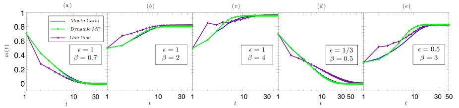
Figure 4: Color online. Comparison between dynamic message passing algorithm (solid lines with $\bullet$ dots), one-time approximation (solid lines with $\scriptstyle\blacklozenge$ dots) and Monte Carlo simulation (solid lines) for the evolution of the magnetization $m(t)$ in an in an Erdös Rényi network of $N=5000$ nodes and average connectivity $c=3$. (a), (b) and (c)-plot: fully symmetric network at high and low temperatures. (d) and (e)-plot: partially symmetric networks with different connectivity symmetry at high and low temperatures. In MC simulations $m(t)$ is averaged over 5000 samples.

We conclude this section underling that we expect improvement of the results provided by the dynamic message-passing scheme presented, both for the transient and for the stationary or equilibrium state, when a higher order closure of the DMP equations is made (see next section).

VI Higher order closures

To close (3) in the class of $n$-th order Markov processes we consider, instead of $P_{i\to(ij)}^{(t-1)}$ and $P_{i\to(ij)}^{(t,t-1)}$ in (10) and (11), the marginalizations $P_{i\to(ij)}^{(t-1,t-2,\ldots,t-n)}$ and $P_{i\to(ij)}^{(t,t-1,t-2,\ldots,t-n)}$ and auxiliary functions $F^{(n)}$ and $G^{(n)}$ which depend on $n$ earlier times. The time iteration of $F^{(n)}$, $G^{(n)}$ and the iterative solution of the $n$-th order kernel $T^{(n)}_{i\to(ij)}(\sigma_{i}|\sigma_{i}^{{}^{\prime}},\sigma_{j}^{{}^{\prime}},\ldots,\sigma_{i}(t-n),\sigma_{j}(t-n))$ then proceed analogously to above. The computational cost obviously increases quickly with $n$ and the value of higher order closures will depend on the application and the model. This issue will be addressed in future contributions.

VII Acknowledgements

The authors acknowledge valuable discussions with Federico Ricci-Tersenghi, Silvio Franz, Haiping Huang, Andrey Y. Lokhov, Yoshiyuki Kabashima and Gabriele Perugini. This work was finalized during the program ”Collective Dynamics in Information System” at Kavli Institute for Theoretical Physics China (KITPC) in Beijing, China. It has been funded under FP7/2007-2013/grant agreement n 290038 (GDF) and supported by the Swedish Science Council through grant 621-2012-2982 and by the Academy of Finland through its Center of Excellence COIN (EA).

References

- [1] Andrea Crisanti and Luca Leuzzi. Amorphous-amorphous transition and the two-step replica symmetry breaking phase. Physical Review B, 76(18):184417, 2007.
- [2] Richard A Goldstein, Zaida A Luthey-Schulten, and Peter G Wolynes. Optimal protein-folding codes from spin-glass theory. Proceedings of the National Academy of Sciences, 89(11):4918–4922, 1992.
- [3] Giuseppe Facchetti, Giovanni Iacono, and Claudio Altafini. Computing global structural balance in large-scale signed social networks. Proceedings of the National Academy of Sciences, 108(52):20953–20958, 2011.
- [4] Scott Kirkpatrick, Alex Kulakovsky, Manuel Cebrian, and Alex “Sandy” Pentland. Social networks and spin glasses. Philosophical Magazine, 92(1-3):362–377, 2012.
- [5] Romualdo Pastor-Satorras and Alessandro Vespignani. Epidemic spreading in scale-free networks. Physical review letters, 86(14):3200, 2001.
- [6] Daniel J Amit. Modeling brain function: The world of attractor neural networks. Cambridge University Press, 1992.
- [7] Anthony CC Coolen. The Mathematical Theory of Minority Games: Statistical Mechanics of Interacting Agents (Oxford Finance Series). Oxford University Press, Inc., 2005.
- [8] Marc Mézard, Giorgio Parisi, and Riccardo Zecchina. Analytic and algorithmic solution of random satisfiability problems. Science, 297(5582):812–815, 2002.
- [9] Silvio Franz, Michele Leone, Federico Ricci-Tersenghi, and Riccardo Zecchina. Exact solutions for diluted spin glasses and optimization problems. Phys. Rev. Lett., 87:127209, Aug 2001.
- [10] Dimitris Achlioptas. Algorithmic barriers from phase transitions in graphs. In Graph Theoretic Concepts in Computer Science, pages 1–1. Springer, 2010.
- [11] Jean-Philippe Bouchaud, Leticia F Cugliandolo, Jorge Kurchan, and Marc Mezard. Out of equilibrium dynamics in spin-glasses and other glassy systems. arXiv preprint cond-mat/9702070, 1997.
- [12] Marc Mezard and Andrea Montanari. Information, physics, and computation. Oxford University Press, 2009.
- [13] H.J. Kappen and FB Rodriguez. Efficient learning in boltzmann machines using linear response theory. Neural. Comput., 10(5):1137–1156, 1998.
- [14] HJ Kappen and JJ Spanjers. Mean field theory for asymmetric neural networks. Physical Review E, 61(5):5658, 2000.
- [15] C De Dominicis. Dynamics as a substitute for replicas in systems with quenched random impurities. Physical Review B, 18(9):4913, 1978.
- [16] H Sompolinsky and A Zippelius. Relaxational dynamics of the Edwards-Anderson model and the mean-field theory of spin-glasses. Physical Review B, 25(11), 1982.
- [17] Hans-Jürgen Sommers. Path-integral approach to ising spin-glass dynamics. Physical review letters, 58(12):1268, 1987.
- [18] Y. Roudi and J. Hertz. Dynamical tap equations for non-equilibrium ising spin glasses. J. Stat. Mech., page P03031, 2011.
- [19] Gino Del Ferraro and Erik Aurell. Perturbative large deviation analysis of non-equilibrium dynamics. Journal of the Physical Society of Japan, 83(8):084001, 2014.
- [20] D.T. Gillespie. Exact stochastic simulation of coupled chemical reactions. J. Phys. Chem., 81(25):2340–2361, 1977.
- [21] Jonathan S Yedidia, William T Freeman, and Yair Weiss. Understanding belief propagation and its generalizations. Exploring artificial intelligence in the new millennium, 8:236–239, 2003.
- [22] B Derrida, E Gardner, and A Zippelius. An exactly solvable asymmetric neural network model. EPL (Europhysics Letters), 4(2):167, 1987.
- [23] M. Mezard and J. Sakellariou. Exact mean-field inference in asymmetric kinetic ising systems. J. Stat. Mech., page L07001, 2011.
- [24] Erik Aurell and Hamed Mahmoudi. Three lemmas on dynamic cavity method. Communications in Theoretical Physics, 56(1):157, 2011.
- [25] Yashodhan Kanoria and Andrea Montanari. Majority dynamics on trees and the dynamic cavity method. The Annals of Applied Probability, 21(5):1694–1748, October 2011.
- [26] Hiroki Ohta and Shin-ichi Sasa. A universal form of slow dynamics in zero-temperature random-field ising model. EPL (Europhysics Letters), 90(2):27008, 2010.
- [27] Fabrizio Altarelli, Alfredo Braunstein, L Dall Asta, and Riccardo Zecchina. Large deviations of cascade processes on graphs. Physical Review E, 87(6):062115, 2013.
- [28] Fabrizio Altarelli, Alfredo Braunstein, Luca Dall’Asta, and Riccardo Zecchina. Optimizing spread dynamics on graphs by message passing. Journal of Statistical Mechanics: Theory and Experiment, 2013(09):P09011, 2013.
- [29] Andrey Y Lokhov, Marc Mézard, Hiroki Ohta, and Lenka Zdeborová. Inferring the origin of an epidemic with dynamic message-passing algorithm. arXiv preprint arXiv:1303.5315, 2013.
- [30] Andrey Y Lokhov, Marc Mézard, and Lenka Zdeborová. Dynamic message-passing equations for models with unidirectional dynamics. arXiv preprint arXiv:1407.1255, 2014.
- [31] I Neri and D Bollé. The cavity approach to parallel dynamics of Ising spins on a graph. Journal of Statistical Mechanics: Theory and Experiment, 2009(08):P08009, August 2009.
- [32] Erik Aurell and Hamed Mahmoudi. A message-passing scheme for non-equilibrium stationary states. Journal of Statistical Mechanics: Theory and Experiment, 2011(04):P04014, 2011.
- [33] Erik Aurell and Hamed Mahmoudi. Dynamic mean-field and cavity methods for diluted ising systems. Physical Review E, 85(3):031119, 2012.
- [34] Alessandro Pelizzola. Variational approximations for stationary states of ising-like models. The European Physical Journal B, 86(4), 2013.
- [35] JPL Hatchett, B Wemmenhove, I Pérez Castillo, T Nikoletopoulos, NS Skantzos, and ACC Coolen. Parallel dynamics of disordered ising spin systems on finitely connected random graphs. Journal of Physics A: Mathematical and General, 37(24):6201, 2004.