Proceedings of the Second Annual LHCP

Implementation and validation of the LHC SUSY searches with MadAnalysis 5

Béranger Dumont

LPSC, Université Grenoble-Alpes, CNRS/IN2P3,
53 Avenue des Martyrs, F-38026 Grenoble, France

ABSTRACT

Separate, validated implementations of the ATLAS and CMS new physics analyses are necessary to fully exploit the potential of these searches. To this end, we use MadAnalysis 5, a public framework for collider phenomenology. In this talk, we present recent developments of MadAnalysis 5, as well as a new public database of reimplemented LHC analyses. The validation of one ATLAS and one CMS search for supersymmetry, present in the database, is also summarized.

PRESENTED AT

The Second Annual Conference

on Large Hadron Collider Physics

Columbia University, New York, U.S.A

June 2-7, 2014

1 Introduction

The ATLAS and CMS collaborations have performed a large number of searches for new physics during Run I of the LHC, targeting in particular supersymmetry in analyses based on missing transverse momentum. The implications of the (so far) negative results for new physics go well beyond the interpretations given in the experimental papers. Separate, validated implementations of the analyses using public fast simulation tools are necessary for theorists to fully exploit the potential of these searches. This will also give useful feedback to the experiments on the impact of their searches.

Recent developments of MadAnalysis 5 [1, 2], the framework we use for reimplementing analyses, are presented in Section 2. The public database of reimplemented LHC analyses is then introduced in Section 3. Finally, a summary of the validation of one ATLAS and one CMS search for supersymmetry (SUSY) can be found in Sections 4 and 5, and conclusions are given in Section 6.

2 New developments in MadAnalysis 5

In most experimental analyses performed at the LHC, and in particular the searches considered in this work, a branching set of selection criteria (“cuts”) is used to define several different sub-analyses (“regions”) within the same analysis. In conventional coding frameworks, multiple regions are implemented with a nesting of conditions checking these cuts, which grows exponentially more complicated with the number of cuts. The scope of this project has therefore motivated us to extend the MadAnalysis 5 package to facilitate the handling of analyses with multiple regions, as described in detail in [1].

From version 1.1.10 onwards, the implementation of an analysis in the MadAnalysis 5 framework consists of implementing three basic functions: i) Initialize, dedicated to the initialization of the signal regions, histograms, cuts and any user-defined variables; ii) Execute, containing the analysis cuts and weights applied to each event; and iii) Finalize, controlling the production of the results of the analysis, i.e., histograms and cut-flow charts. To illustrate the handling of multiple regions, we present a few snippets of our implementation [3] of the CMS search for stops in final states with one lepton [4] (see Section 5). This search comprises 16 signal regions (SRs), all of which must be declared in the Initialize function. This is done through the AddRegionSelection method of the analysis manager class, of which Manager() is an instance provided by default with each analysis. It takes as its argument a string uniquely defining the SR under consideration. For instance, two of the 16 SRs of the CMS analysis are declared as

 Manager()->AddRegionSelection("Stop->t+neutralino,LowDeltaM,MET>150");
 Manager()->AddRegionSelection("Stop->t+neutralino,LowDeltaM,MET>200");

The Initialize function should also contain the declaration of selection cuts. This is handled by the AddCut method of the analysis manager class. If a cut is common to all SRs, the AddCut method takes as a single argument a string that uniquely identifies the cut. An example of the declaration of two common cuts is

 Manager()->AddCut("1+ candidate lepton");
 Manager()->AddCut("1 signal lepton");

If a cut is not common to all regions, the AddCut method requires a second argument, either a string or an array of strings, consisting of the names of all the regions to which the cut applies. For example, an $E_{T}^{\rm miss}>150$ GeV cut that applies to four SRs could be declared as

 string SRForMet150Cut[] = {"Stop->b+chargino,LowDeltaM,MET>150",
                            "Stop->b+chargino,HighDeltaM,MET>150",
                            "Stop->t+neutralino,LowDeltaM,MET>150",
                            "Stop->t+neutralino,HighDeltaM,MET>150"};
 Manager()->AddCut("MET>150GeV",SRForMet150Cut);

Histograms are initialized in a similar fashion using the AddHisto method of the manager class. A string argument is hence required to act as a unique identifier for the histogram, provided together with its number of bins and bounds. A further optional argument consisting of a string or array of strings can then be used to associate it with specific regions. The exact syntax can be found in the manual [1].

Most of the logic of the analysis is implemented in the Execute function. This relies both on standard methods to declare particle objects and to compute the observables of interest for event samples including detector simulation [2] and on the new manner in which cuts are applied and histograms filled via the analysis manager class [1]. Below we provide a couple of examples for applying cuts and filling histograms. After having declared and filled two vectors, SignalElectrons and SignalMuons, with objects satisfying the signal lepton definitions used in the CMS-SUS-13-011 analysis, we require exactly one signal lepton with the following selection cut:

 if( !Manager()->ApplyCut( (SignalElectrons.size()+SignalMuons.size())>0,
   "1+ candidate lepton") ) return true;

The if(...) syntax guarantees that a given event is discarded as soon as all regions fail the cuts applied so far. Histogramming is as easy as applying a cut. For example, as we are interested in the transverse-momentum distribution of the leading lepton, our code contains

 Manager()->FillHisto("pT(l)",SignalLeptons[0]->pt());

This results in the filling of a histogram, previously declared with the name "pT(l)" in the Initialize method, but only when all cuts applied to the relevant regions are satisfied.

After the execution of the program, a set of Saf files (an Xml-inspired format used by MadAnalysis 5) is created. They contain general information on the analyzed events, as well as the cut-flow tables for all SRs and the histograms. The structure of the various Saf files is detailed in [1].

3 Public analysis database of LHC new physics searches

A public database of reimplemented analyses in the MadAnalysis 5 framework and using Delphes 3 [5] was presented in [6]. The list of analyses presently available in the database can be found on the wiki page [7]. Each analysis code, in the C++ language used in MadAnalysis 5, is submitted to INSPIRE, hence is searchable and citeable. The information on the number of background and observed events is required for setting limits and is provided in the form of an Xml file that is submitted to INSPIRE together with the analysis code. Finally, detector tunings (contained in the detector card for Delphes) as well as detailed validation results for each analysis can be found on the wiki page. To date, there are five SUSY analyses in the database, two from ATLAS and three from CMS.

From an event file in StdHep or HepMc format, the acceptance$\times$efficiency can be found in the output of MadAnalysis 5 for each SR. The limit setting can subsequently done under the CL_s prescription with the code exclusion_CLs.py. It reads the cross section and the acceptance$\times$efficiency from the output of MadAnalysis 5, while the luminosity and the required information on the signal regions is taken from the Xml file mentioned above.

4 ATLAS-SUSY-2013-05: search for third-generation squarks in final states with zero leptons and two $b$-jets

In this ATLAS analysis [8], stops and sbottoms are searched for in final states with large missing transverse momentum and two jets identified as $b$-jets. The results are presented for an integrated luminosity of $20.1$ fb^-1 at $\sqrt{s}=8$ TeV. Two possible sets of SUSY mass spectra were investigated in this analysis: i) sbottom $\tilde{b}_{1}$ pair production with $\tilde{b}_{1}\rightarrow b\tilde{\chi}_{1}^{0}$, and ii) stop $\tilde{t}_{1}$ pair production with $\tilde{t}_{1}\rightarrow b\tilde{\chi}_{1}^{\pm}$, where the subsequent decay of the $\tilde{\chi}_{1}^{\pm}$ is invisible due to a small mass splitting with the $\tilde{\chi}_{1}^{0}$. Two sets of SRs, SRA and SRB, are defined to provide sensitivity to respectively large and small mass splittings between the squark and the neutralino.

	$m_{\tilde{b}_{1}}=350$ GeV		$m_{\tilde{t}_{1}}=500$ GeV
cut	ATLAS result	MA 5 result	ATLAS result	MA5 result
$E^{\rm miss}_{T}>80$ GeV filter	$6221.0$	$5963.7$	$1329.0$	$1117.9$
+ Lepton veto	$4069.0$	$4987.9$	$669.0$	$932.9$
+ $E^{\rm miss}_{T}>250$ GeV	$757.0$	$802.9$	$93.0$	$117.2$
+ Jet Selection	$7.9$	$5.4$	$6.2$	$5.3$
+ $H_{T,3}<50$ GeV	$5.2$	$4.6$	$3.0$	$4.2$

Table 1: Summary of yields for SRB of ATLAS-SUSY-2013-05 corresponding to the benchmark points $(m_{\tilde{b}_{1}},m_{\tilde{\chi}^{0}_{1}})=(350,320)$ GeV and $(m_{\tilde{t}_{1}},m_{\tilde{\chi}^{\pm}_{1}},m_{\tilde{\chi}^{0}_{1}})=(500,420,400)$ GeV, as compared to official ATLAS results given on [8]. An $E^{\rm miss}_{T}$ filter is applied at the particle level. See [8] for more detail.

The analysis is very well documented regarding physics, but for recasting purposes more information than provided in [8] was needed. This made the validation of the recast code seriously difficult in the earlier stages of the project. Since then, fortunately, cut-flow tables were made public, as well as SUSY Les Houches Accord (SLHA) input files and the exact version of Monte Carlo tools used to generate the signal. However, the collaboration did not provide information on trigger-only and $b$-tagging efficiencies.

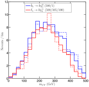
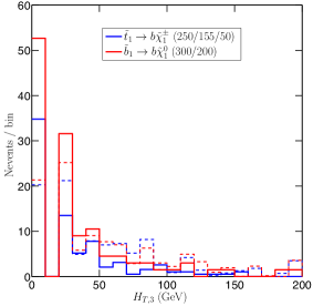
Figure 1: Distributions of $m_{CT}$ for SRA and $H_{T,3}$ for SRB of ATLAS-SUSY-2013-05 without their respective cut. On the left plot, the benchmark points used are $(m_{\tilde{b}_{1}},m_{\tilde{\chi}_{1}^{0}})$ = $(500,1)$ GeV (in blue) and $(m_{\tilde{t}_{1}},m_{\tilde{\chi}^{\pm}_{1}},m_{\tilde{\chi}^{0}_{1}})$ = $(500,105,100)$ GeV (in red). On the right plot, $(m_{\tilde{t}_{1}},m_{\tilde{\chi}^{\pm}_{1}},m_{\tilde{\chi}^{0}_{1}})$ = $(250,155,50)$ GeV (in blue) and $(m_{\tilde{b}_{1}},m_{\tilde{\chi}_{1}^{0}})$ = $(300,200)$ GeV (in red). The solid lines correspond to our re-interpretation within MadAnalysis 5 and the dashed lines to the ATLAS result.

The comparison between the official cut flows and the ones obtained within MadAnalysis 5 is presented in the case of SRB in Table 1. Moreover, distributions of the contransverse variable $m_{CT}$ and of $H_{T,3}$ are shown in Fig. 1. ($H_{T,3}$ is defined as the sum of the $p_{T}$ of the $n$ jets without including the leading three jets.) The largest discrepancy is observed in SRB, as be seen in the distribution of $H_{T,3}$. To investigate this issue more deeply, a more detailed cut flow about the “Jet selection” line in Table 1 would be appreciable since it directly impacts the $H_{T,3}$ variable.

Overall the agreement is quite satisfactory, considering the expected accuracy for a fast simulation. For SRA the agreement is very good. For SRB, the importance of the treatment of soft jets induces a sizable discrepancy with respect to the ATLAS results. Further tunings of the fast detector simulation are needed, and are currently under investigation. However, the current results (for which detailed validation material can be found at [7]) lead us to conclude that this implementation is validated. The MadAnalysis 5 recast code is available as [9].

5 CMS-SUS-13-011: search for stops in the single-lepton final state

The CMS search for stops in the single lepton and missing energy, $\ell+E^{\rm miss}_{T}$, final state with full luminosity at $\sqrt{s}=8$ TeV [4] has been taken as a “template analysis” to develop a common language and framework for the analysis implementation. The analysis targets two possible decay modes of the stop: $\tilde{t}\to t\tilde{\chi}^{0}_{1}$ and $\tilde{t}\to b\tilde{\chi}^{+}_{1}$. Since the stops are pair-produced, their decays give rise to two $W$ bosons in each event, one of which is assumed to decay leptonically, while the other one is assumed to decay hadronically. In the cut-based version of the analysis, that we consider, two sets of signal regions with different cuts, each dedicated to one of the two decay modes, are defined. These two sets are further divided into “low $\Delta M$” and “high $\Delta M$” categories, targeting small and large mass differences with the lightest neutralino $\tilde{\chi}_{1}^{0}$, respectively. Finally, each of these four categories are further sub-divided using four different $E^{\rm miss}_{T}$ requirements. In total, 16 different, potentially overlapping SRs are defined.

Overall, this analysis is well documented. Detailed trigger efficiencies and the identification-only efficiencies for electron and muons were provided by the CMS collaboration upon request and are now available on the analysis Twiki page [4] in the section “Additional Material to aid the Phenomenology Community with Reinterpretations of these Results”. The $b$-tagging efficiency as a function of $p_{T}$ was taken from [10]. Another technical difficulty came from the isolation criteria. Since we used a simplified isolation criteria, we applied on the events a weighting factor of $0.885$ that was determined from the two cut flows (see Table 2).

The validation was done using the eleven benchmark points presented in the experimental paper. The validation process was based on (partonic) event samples, in LHE format, provided by the CMS collaboration. Some examples of histograms reproduced for the validation are shown in Fig. 2. The shapes of the distributions shown—as well as all other distributions that we obtained but do not show here—follow closely the ones from CMS, which indicates the correct implementation of the analysis and all the kinematic variables.

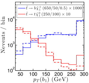
Figure 2: Distributions of $M^{W}_{T2}$ (left) and of the $p_{T}$ of the leading $b$-tagged jet (right) after the preselection cuts of the analysis CMS-SUS-13-011. The solid lines are obtained from our re-interpretation within MadAnalysis 5, while the dash-dotted lines correspond to the CMS results, given in Fig. 2 of [4].

Upon our request, the CMS SUSY group furthermore provided detailed cut-flow tables, which are now also available on the Twiki page of the analysis [4]. These proved extremely useful because they allowed us to verify our implementation step-by-step in the analysis. A comparison of our results with the official CMS ones is given in Table 2. For both cases shown, CMS results are reproduced within about 20%. On the whole, we conclude that our implementation gives reasonably accurate results (to the level that can be expected from fast simulation). The MadAnalysis 5 code for this analysis, including extensive comments, is published as [3].

	$m_{\tilde{t}}=650$ GeV		$m_{\tilde{t}}=250$ GeV
cut	CMS result	MA 5 result	CMS result	MA5 result
$1\ell\,+\geq 4{\rm jets}+E_{T}^{\rm miss}>50$ GeV	$31.6\pm 0.3$	$29.0$	$8033.0\pm 38.7$	$7365.0$
+ $E_{T}^{\rm miss}>100$ GeV	$29.7\pm 0.3$	$27.3$	$4059.2\pm 27.5$	$3787.2$
+ $n_{b}\geq 1$	$25.2\pm 0.2$	$23.8$	$3380.1\pm 25.1$	$3166.0$
+ iso-track veto	$21.0\pm 0.2$	$19.8$	$2770.0\pm 22.7$	$2601.4$
+ tau veto	$20.6\pm 0.2$	$19.4$	$2683.1\pm 22.4$	$2557.2$
+ $\Delta\phi_{\rm min}>0.8$	$17.8\pm 0.2$	$16.7$	$2019.1\pm 19.4$	$2021.3$
+ hadronic $\chi^{2}<5$	$11.9\pm 0.2$	$9.8$	$1375.9\pm 16.0$	$1092.0$
+ $M_{T}>120$ GeV	$9.6\pm 0.1$	$7.9$	$355.1\pm 8.1$	$261.3$
${\rm high\,}\Delta M,E^{\rm miss}_{T}>300~{}{\rm GeV}$	$4.2\pm 0.1$	$3.9$	—	—
${\rm low\,}\Delta M,E^{\rm miss}_{T}>150~{}{\rm GeV}$	—	—	$124.0\pm 4.8$	$107.9$

Table 2: Summary of yields for the $\tilde{t}\rightarrow t\tilde{\chi}^{0}_{1}$ model for two benchmark points with $m_{\tilde{\chi}^{0}_{1}}=50$ GeV, as compared to official CMS-SUS-13-011 results given on [4]. The uncertainties given for the CMS event numbers are statistical only. See [4] for more details on the definition of the cuts.

6 Conclusions

We presented recent developments of MadAnalysis 5 that were necessary for the implementation and for recasting LHC new physics analyses. After validation, reimplemented analyses are stored in a new public database. We discussed the validation of two SUSY analyses. A growing number of such analysis codes, including detailed validation material, is being made available in a public analysis database, see [7].

ACKNOWLEDGEMENTS

I am grateful to the ATLAS and CMS collaborations for their help in validating the results. I would also like to thank my colleagues of [1] and [6] for their collaboration and for inspiring discussions.

References

- [1] E. Conte, B. Dumont, B. Fuks and C. Wymant, arXiv:1405.3982 [hep-ph].
- [2] E. Conte, B. Fuks and G. Serret, Comput. Phys. Commun. 184 (2013) 222 [arXiv:1206.1599 [hep-ph]].
- [3] B. Dumont, B. Fuks, and C. Wymant, doi: 10.7484/INSPIREHEP.DATA.LR5T.2RR3.
- [4] S. Chatrchyan et al. [CMS Collaboration], Eur. Phys. J. C 73 (2013) 2677 [arXiv:1308.1586 [hep-ex]]; https://twiki.cern.ch/twiki/bin/view/CMSPublic/PhysicsResultsSUS13011.
- [5] J. de Favereau et al. [DELPHES 3 Collaboration], JHEP 1402 (2014) 057 [arXiv:1307.6346 [hep-ex]].
- [6] B. Dumont, B. Fuks, S. Kraml, et al., arXiv:1407.3278 [hep-ph].
- [7] http://madanalysis.irmp.ucl.ac.be/wiki/PhysicsAnalysisDatabase.
-
[8]
G. Aad et al. [ATLAS Collaboration],
JHEP 1310 (2013) 189
[arXiv:1308.2631 [hep-ex]];
https://atlas.web.cern.ch/Atlas/GROUPS/PHYSICS/PAPERS/SUSY-2013-05/. - [9] G. Chalons, doi: 10.7484/INSPIREHEP.DATA.Z4ML.3W67.
- [10] S. Chatrchyan et al. [CMS Collaboration], JHEP 1401 (2014) 163 [arXiv:1311.6736 [hep-ex]].