Initialization-free distributed coordination for economic dispatch under varying loads and generator commitment

Abstract

This paper considers the economic dispatch problem for a network of power generating units communicating over a strongly connected, weight-balanced digraph. The collective aim is to meet a power demand while respecting individual generator constraints and minimizing the total generation cost. We design a distributed coordination algorithm consisting of two interconnected dynamical systems. One block uses dynamic average consensus to estimate the evolving mismatch in load satisfaction given the generation levels of the units. The other block adjusts the generation levels based on the optimization objective and the estimate of the load mismatch. Our convergence analysis shows that the resulting strategy provably converges to the solution of the dispatch problem starting from any initial power allocation, and therefore does not require any specific procedure for initialization. We also characterize the algorithm robustness properties against the addition and deletion of units (capturing scenarios with intermittent power generation) and its ability to track time-varying loads. Our technical approach employs a novel refinement of the LaSalle Invariance Principle for differential inclusions, that we also establish and is of independent interest. Several simulations illustrate our results.

1 Introduction

The advent of renewable energy sources and their integration into electricity grids is making power generation and distribution an increasingly decentralized problem. The large-scale and highly dynamic nature of the resulting grid optimization problems makes traditional centralized, top-down approaches impractical because they rely on the assumption of a fixed, limited number of generation units. To solve these problems efficiently, there is a need to design distributed algorithms that can handle dynamic loads, provide plug-and-play capabilities, are robust against transmission and generation failures, and adequately preserve the privacy of the entities involved. These considerations motivate us to consider here the design of distributed algorithmic solutions to the economic dispatch (ED) problem, where a group of power generators aims to meet a power demand while minimizing the total generation cost (the summation of individual costs) and respecting the individual generators’ capacity constraints. We are interested in the synthesis of strategies that solve the ED problem starting from any initial power allocation, can handle time-varying loads, and are robust against intermittent power generation caused by unit addition and deletion.

Literature review: The ED problem has been traditionally solved in a centralized manner, see e.g. (Chowdhury and Rahman, 1990) and references therein. Since distributed algorithmic solutions to grid optimization problems are envisioned as part of the future smart grid (Farhangi, 2010), this has motivated the appearance of a number of distributed strategies for the ED problem in the literature. While there exists a broad variety in the assumptions made, a majority of the works rely on the specific form of the solutions of the optimization problem and propose consensus-based algorithms. Many works consider convex, quadratic cost functions for the power generators and perform consensus over their incremental costs under undirected (Zhang and Chow, 2012; Kar and Hug, 2012) or directed (Dominguez-Garcia et al., 2012; Binetti et al., 2014a) communication topologies. Some works consider general convex cost functions, like we do here, but either do not consider capacity constraints on the generators (Mudumbai et al., 2012), assume the initial power allocation to meet the total load (Cherukuri and Cortés, 2013; Pantoja et al., 2014), or require feedback on the power mismatch from the shift in frequency due to primary droop control (Zhang et al., 2014). Along with load and capacity constraints, Binetti et al. (2014a); Loia and Vaccaro (2013) consider transmission losses, and Binetti et al. (2014b) additionally take into account valve-point loading effects and prohibited operating zones. However, these constraints make the problem nonconvex and prevent these works from obtaining theoretical guarantees on the algorithm convergence properties. In (Du et al., 2012), the authors propose best-response dynamics for a potential-game formulation of the nonconvex ED problem, but the implementation requires all-to-all communication among the generators. Xiao and Boyd (2006); Johansson and Johansson (2009) introduce distributed methods to solve resource allocation problem very similar to the ED problem, but without taking into account individual agent constraints. Instead, these are incorporated in the formulation of Simonetto et al. (2012), but the proposed algorithm arrives at suboptimal solutions of the optimization problem. Our algorithm design and analysis rely on dynamic average consensus and differential inclusions. In dynamic average consensus, see e.g. (Freeman et al., 2006; Kia et al., 2014) and references therein, each agent has access to a time-varying input signal and interacts with its neighbors in order to track the average of the input signals across the network. We build on our previous work (Cherukuri and Cortés, 2013), which requires a proper algorithm initialization, and employ tools from dynamic average consensus to synthesize a coordination strategy that converges from any initial condition. Regarding analysis, our technical approach builds on Lyapunov stability tools for differential inclusions and nonsmooth systems, see e.g. (Bacciotti and Ceragioli, 1999; Cortés, 2008) and references therein. Of particular importance is the work (Arsie and Ebenbauer, 2010) for differential equations, that provides a way to further refine the description of omega-limit sets of trajectories by employing more than one LaSalle-type function.

Statement of contributions: We start with the formal definition of the ED problem for a network of power generators communicating over a strongly connected, weight-balanced digraph. The optimization problem is convex as the individual cost functions are smooth and convex, the load satisfaction is a linear constraint, and the individual generators’ capacities prescribe convex inequality constraints. Our formulation is a simplification of the ED problem in its full generality, which in practice may have additional constraints (e.g., transmission losses, line capacity constraints, valve-point loading effects, ramp rate limits, prohibited operating zones) that make it nonconvex. However, our developments show that obtaining a provably correct algorithmic solution for the formulation here of the ED problem given our performance requirements (distributed, convergent irrespective of initial condition, able to handle time-varying loads, and robust to intermittent power generation) is challenging. Our first contribution is the design of a centralized algorithm, termed “load mismatch + Laplacian-nonsmooth-gradient” dynamics, that solves the ED problem starting from any initial power allocation. This strategy has two components: one component seeks to optimize the network generation cost while keeping constant the total power generated; the other component is a feedback correction term driven by the error between the desired total load and the network generation. This latter term is responsible for ensuring that the algorithm trajectories asymptotically satisfy the load satisfaction constraint irrespective of the initial power allocation. These observations set the basis for our second contribution, which is the synthesis of a distributed coordination algorithm, termed “dynamic average consensus + Laplacian-nonsmooth-gradient” dynamics, with the same convergence guarantees. Our design consists of two coupled dynamical systems: a dynamic average consensus algorithm to estimate the mismatch between generation and desired load in a distributed fashion and a distributed Laplacian-nonsmooth-gradient dynamics that employs these estimates to dynamically allocate the unit generation levels. The convergence analysis of both the centralized and distributed algorithms relies on a combination of tools from algebraic graph theory, nonsmooth analysis, set-valued dynamical systems, and dynamic average consensus, and most notably on a refined version of the LaSalle Invariance Principle for differential inclusions, which constitutes our third contribution. Roughly speaking, the application of the known LaSalle Invariance Principle would only establish asymptotic convergence towards the network satisfaction of the total load. Instead, the use of the refined version allows us, for each algorithm, to establish global convergence of the trajectories to the solutions of the ED problem. Our final contribution is the formal characterization of the robustness properties of the distributed algorithm. Building on the observation that the mismatch dynamics between network generation and total load is exponentially convergent and input-to-state stable, we establish the algorithm ability to track time-varying loads and its robustness in scenarios with intermittent power generation.

2 Preliminaries

This section introduces basic concepts and preliminaries. We begin with some notational conventions. Let ${\mathbb{R}}$, ${\mathbb{R}}_{\geq 0}$, ${\mathbb{R}}_{>0}$, $\mathbb{Z}_{\geq 1}$ denote the real, nonnegative real, positive real, and positive integer numbers, resp. For $r\in{\mathbb{R}}$ we denote $\mathcal{H}_{r}=\{x\in{\mathbb{R}}^{n}\;|\;\mathbf{1}_{n}^{\top}x=r\}$. The $2$- and $\infty$-norms on ${\mathbb{R}}^{n}$ and their respective induced norms on ${\mathbb{R}}^{n\times n}$ are denoted with $\|\cdot\|$ and $\|\cdot\|_{\infty}$, resp. We let $B(x,\delta)=\{y\in{\mathbb{R}}^{n}\;|\;\|y-x\|<\delta\}$. For $D\subset{\mathbb{R}}^{n}$, $\overline{D}$ denotes its closure. For $x\in{\mathbb{R}}^{n}$, $x_{i}\in{\mathbb{R}}$ denotes its $i$-th component. Given vectors $x,y\in{\mathbb{R}}^{n}$, $x\leq y$ if and only if $x_{i}\leq y_{i}$ for all $i\in\{1,\dots,n\}$. We denote $\mathbf{1}_{n}=(1,\ldots,1)\in{\mathbb{R}}^{n}$.A set-valued map $f:{\mathbb{R}}^{n}\rightrightarrows{\mathbb{R}}^{m}$ associates to each point in ${\mathbb{R}}^{n}$ a set in ${\mathbb{R}}^{m}$. For a symmetric matrix $A\in{\mathbb{R}}^{n\times n}$, $\lambda_{\min}(A)$ and $\lambda_{\max}(A)$ denote the minimum and maximum eigenvalues of $A$. Finally, we let $[u]^{+}=\max\{0,u\}$ for $u\in{\mathbb{R}}$.

2.1 Graph theory

We present basic notions from algebraic graph theory following (Bullo et al., 2009). A directed graph (or digraph) is a pair $\mathcal{G}=(\mathcal{V},\mathcal{E})$, with $\mathcal{V}=\{1,\dots,n\}$ the vertex set and $\mathcal{E}\subseteq\mathcal{V}\times\mathcal{V}$ the edge set. A path is a sequence of vertices connected by edges. A digraph is strongly connected if there is a path between any pair of vertices. The sets of out- and in-neighbors of $v$ are, resp., $N^{\textup{out}}(v)=\{w\in\mathcal{V}\;|\;(v,w)\in\mathcal{E}\}$ and $N^{\textup{in}}(v)=\{w\in\mathcal{V}\;|\;(w,v)\in\mathcal{E}\}$. A weighted digraph $\mathcal{G}=(\mathcal{V},\mathcal{E},\mathsf{A})$ is composed of a digraph $(\mathcal{V},\mathcal{E})$ and an adjacency matrix $\mathsf{A}\in\mathbb{R}^{n\times n}_{\geq 0}$ with $a_{ij}>0$ iff $(i,j)\in\mathcal{E}$. The weighted out- and in-degree of $i$ are, resp., $d^{\textup{out}}(i)=\sum_{j=1}^{n}a_{ij}$ and $d^{\textup{in}}(i)=\sum_{j=1}^{n}a_{ji}$. The Laplacian matrix is $\mathsf{L}=\mathsf{D}_{\textup{out}}-\mathsf{A}$, where $\mathsf{D}_{\textup{out}}$ is the diagonal matrix with $(\mathsf{D}_{\textup{out}})_{ii}=d^{\textup{out}}(i)$, for all $i\in\{1,\ldots,n\}$. Note that $\mathsf{L}\mathbf{1}_{n}=0$. If $\mathcal{G}$ is strongly connected, then $0$ is a simple eigenvalue of $\mathsf{L}$. $\mathcal{G}$ is undirected if $\mathsf{L}=\mathsf{L}^{\top}$. $\mathcal{G}$ is weight-balanced if $d^{\textup{out}}(v)=d^{\textup{in}}(v)$, for all $v\in\mathcal{V}$ iff $\mathbf{1}_{n}^{\top}\mathsf{L}=0$ iff $\mathsf{L}+\mathsf{L}^{\top}\geq 0$. Note that any undirected graph is weight-balanced. If $\mathcal{G}$ is weight-balanced and strongly connected, then $0$ is a simple eigenvalue of $\mathsf{L}+\mathsf{L}^{\top}$. In such case, one has for $x\in{\mathbb{R}}^{n}$,

$$x^{\top}(\mathsf{L}+\mathsf{L}^{\top})x\geq\lambda_{2}(\mathsf{L}+\mathsf{L}^{\top})\Big{\|}x-\frac{1}{n}(\mathbf{1}_{n}^{\top}x)\mathbf{1}_{n}\Big{\|}^{2},$$ (1)

with $\lambda_{2}(\mathsf{L}+\mathsf{L}^{\top}\!)$ the smallest non-zero eigenvalue of $\mathsf{L}+\mathsf{L}^{\top}\!$.

2.2 Dynamic average consensus

Here, we introduce notions on dynamic average consensus following (Kia et al., 2014). Consider $n\in\mathbb{Z}_{\geq 1}$ agents communicating over a strongly connected, weight-balanced digraph $\mathcal{G}$ whose Laplacian is denoted as $\mathsf{L}$. Each agent is associated with a state $x_{i}\in{\mathbb{R}}$ and an input signal $t\mapsto u_{i}(t)\subset{\mathbb{R}}$ that is measurable and locally essentially bounded. The aim is to provide a distributed dynamics such that the state of each agent $x_{i}(t)$ tracks the average signal $\frac{1}{n}\sum_{i=1}^{n}u_{i}(t)$ asymptotically. This can be achieved via the dynamics $X_{\texttt{dac}}:{\mathbb{R}}^{2n}\rightarrow{\mathbb{R}}^{2n}$,

$$\dot{x} =-\alpha x-\beta\mathsf{L}x-v+\nu u,$$

$$\dot{v} =\alpha\beta\mathsf{L}x,$$

where $\alpha,\beta,\nu>0$ are design parameters and $v\in{\mathbb{R}}^{n}$ is an auxiliary state. If the initial condition satisfies $\mathbf{1}_{n}^{\top}v(0)=0$ and the time-derivatives of the input signals are bounded, then one can show, cf. (Kia et al., 2014, Corollary 4.1), that the error signal $t\mapsto\left\lvert{x_{i}(t)-\frac{1}{n}\sum_{i=1}^{n}u_{i}(t)}\right\rvert$ is ultimately bounded for each $i\in\{1,\dots,n\}$. Moreover, this error vanishes if the input signal converges to a constant value.

2.3 Nonsmooth analysis and differential inclusions

We review here some notions from nonsmooth analysis and differential inclusions following (Cortés, 2008). A function $f:{\mathbb{R}}^{n}\rightarrow{\mathbb{R}}^{m}$ is locally Lipschitz at $x\in{\mathbb{R}}^{n}$ if there exist $L_{x},\epsilon\in(0,\infty)$ such that $\|f(y)-f(y^{\prime})\|\leq L_{x}\|y-y^{\prime}\|$, for all $y,y^{\prime}\in B(x,\epsilon)$. A function $f:{\mathbb{R}}^{n}\rightarrow{\mathbb{R}}$ is regular at $x\in{\mathbb{R}}^{n}$ if, for all $v\in{\mathbb{R}}^{n}$, the right and generalized directional derivatives of $f$ at $x$ in the direction of $v$ coincide, see (Cortés, 2008) for definitions of these notions. A function that is continuously differentiable at $x$ is regular at $x$. Also, a convex function is regular. A set-valued map $\mathcal{H}:{\mathbb{R}}^{n}\rightrightarrows{\mathbb{R}}^{n}$ is upper semicontinuous at $x\in{\mathbb{R}}^{n}$ if, for all $\epsilon\in(0,\infty)$, there exists $\delta\in(0,\infty)$ such that $\mathcal{H}(y)\subset\mathcal{H}(x)+B(0,\epsilon)$ for all $y\in B(x,\delta)$. Also, $\mathcal{H}$ is locally bounded at $x\in{\mathbb{R}}^{n}$ if there exist $\epsilon,\delta\in(0,\infty)$ such that $\|z\|\leq\epsilon$ for all $z\in\mathcal{H}(y)$ and $y\in B(x,\delta)$.

Given a locally Lipschitz function $f:{\mathbb{R}}^{n}\rightarrow{\mathbb{R}}$, let $\Omega_{f}$ be the set (of measure zero) of points where $f$ is not differentiable. The generalized gradient $\partial f:{\mathbb{R}}^{n}\rightrightarrows{\mathbb{R}}^{n}$ is

$$\partial f(x)=\mathrm{co}\{\lim_{i\rightarrow\infty}\nabla f(x_{i})\;|\;x_{i}\rightarrow x,x_{i}\notin S\cup\Omega_{f}\},$$

where $\mathrm{co}$ denotes convex hull and $S\subset{\mathbb{R}}^{n}$ is any set of measure zero. The map $\partial f$ is locally bounded, upper semicontinuous, and takes non-empty, compact, and convex values. A critical point $x$ of $f$ satisfies $0\in\partial f(x)$.

Given a set-valued map $\mathcal{H}:{\mathbb{R}}^{n}\rightrightarrows{\mathbb{R}}^{n}$, a differential inclusion on ${\mathbb{R}}^{n}$ is

$$\dot{x}\in\mathcal{H}(x).$$ (3)

A solution of (3) on $[0,T]\subset{\mathbb{R}}$ is an absolutely continuous map $x:[0,T]\rightarrow{\mathbb{R}}^{n}$ that satisfies (3) for almost all $t\in[0,T]$. If $\mathcal{H}$ is locally bounded, upper semicontinuous, and takes non-empty, compact, and convex values, then existence of solutions is guaranteed. The set of equilibria of (3) is $\mathrm{Eq}(\mathcal{H})=\{x\in{\mathbb{R}}^{n}\;|\;0\in\mathcal{H}(x)\}$. A set $S\subset{\mathbb{R}}^{n}$ is weakly (resp., strongly) positively invariant under (3) if, for each $x\in S$, at least a solution (resp., all solutions) starting from $x$ is (resp., are) entirely contained in $S$. For dynamics with uniqueness of solution, both notions coincide and are referred as positively invariant. Given a locally Lipschitz function $f:{\mathbb{R}}^{n}\rightarrow{\mathbb{R}}$, the set-valued Lie derivative ${\mathcal{L}}_{\mathcal{H}}f:{\mathbb{R}}^{n}\rightrightarrows{\mathbb{R}}$ of $f$ with respect to (3) is

$${\mathcal{L}}_{\mathcal{H}}f(x)=\{a\in{\mathbb{R}}\;|\;\exists v\in\mathcal{H}(x)\text{ s.t. }\zeta^{\top}v=a$$ for all

$$\zeta\in\partial f(x)\}.$$

For a trajectory $t\mapsto\varphi(t)$, $\varphi(0)\in{\mathbb{R}}^{n}$ of (3), the evolution of $f$ along it satisfies

$$\frac{d}{dt}f(\varphi(t))\in{\mathcal{L}}_{\mathcal{H}}f(\varphi(t))$$

for almost all $t\geq 0$. The omega-limit set of the trajectory, denoted $\Omega(\varphi)$, is the set of all points $y\in{\mathbb{R}}^{n}$ for which there exists a sequence $\{t_{k}\}_{k=1}^{\infty}$ with $t_{k}\to\infty$ and $\lim_{k\to\infty}\varphi(t_{k})=y$. If the trajectory is bounded, then the omega-limit set is nonempty, compact, connected, and weakly invariant. These tools allow us to characterize the asymptotic behavior of solutions of differential inclusions. In Appendix A we develop a novel refinement of the LaSalle Invariance Principle for differential inclusions, see e.g., (Cortés, 2008), which is suitable for the analysis of the coordination algorithms.

3 Problem statement

This section presents the network model and the economic dispatch problem we set out to solve in a distributed and robust fashion. Consider $n\in\mathbb{Z}_{\geq 1}$ power generators communicating over a strongly connected and weight-balanced digraph $\mathcal{G}=(\mathcal{V},\mathcal{E},\mathsf{A})$. Each generator corresponds to a vertex in the digraph and an edge $(i,j)$ represents the ability of generator $j$ to send information to generator $i$. The cost of power generation for unit $i$ is measured by $f_{i}:{\mathbb{R}}\rightarrow{\mathbb{R}}_{\geq 0}$, assumed to be convex and continuously differentiable. Representing the power generated by unit $i$ by $P_{i}\in{\mathbb{R}}$, the total cost incurred by the network with the power allocation $P=(P_{1},\dots,P_{n})\in{\mathbb{R}}^{n}$ is measured by $f:{\mathbb{R}}^{n}\rightarrow{\mathbb{R}}_{\geq 0}$ as

$$f(P)=\sum_{i=1}^{n}f_{i}(P_{i}).$$

Note that $f$ is convex and continuously differentiable. The generators aim to minimize the total cost $f(P)$ while meeting the total power load $P_{l}\in{\mathbb{R}}_{>0}$, i.e., $\sum_{i=1}^{n}P_{i}=P_{l}$. Each generator has an upper and a lower limit on the power it can produce, $P_{i}^{m}\leq P_{i}\leq P_{i}^{M}$ for $i\in\{1,\dots,n\}$. Formally, the economic dispatch (ED) problem is

$$\mathrm{minimize}\quad f(P),$$ (4a)

subject to $$\mathbf{1}_{n}^{\top}P=P_{l},$$ (4b)

$$P^{m}\leq P\leq P^{M}.$$ (4c)

The constraint (4b) is the load condition and (4c) are the box constraints. The set of allocations satisfying the box constraints is $\mathcal{F}_{B}=\{P\in{\mathbb{R}}^{n}\;|\;P^{m}\leq P\leq P^{M}\}$. Further, we denote the feasibility set of (4) as $\mathcal{F}_{\mathrm{ED}}=\mathcal{F}_{B}\cap\mathcal{H}_{P_{l}}=\{P\in{\mathbb{R}}^{n}\;|\;P^{m}\leq P\leq P^{M}\text{ and }\mathbf{1}_{n}^{\top}P=P_{l}\}$ and the set of solutions as $\mathcal{F}_{\mathrm{ED}}^{*}$. Since $\mathcal{F}_{\mathrm{ED}}$ is compact, $\mathcal{F}_{\mathrm{ED}}^{*}$ is compact. Note that $P^{M}\in\mathcal{F}_{\mathrm{ED}}$ implies $\mathcal{F}_{\mathrm{ED}}=\{P^{M}\}$. Similarly $P^{m}\in\mathcal{F}_{\mathrm{ED}}$ implies $\mathcal{F}_{\mathrm{ED}}=\{P^{m}\}$. Therefore, we assume $P^{M}$ and $P^{m}$ are not feasible.

Our objective is to design a distributed coordination algorithm that allows the team of generators to solve the ED problem (4) starting from any initial condition, can handle time-varying loads, and is robust to intermittent power generation.

Remark 3.1.

(Additional practical constraints): We do not consider here, for simplicity, other constraints on the ED problem such as transmission losses, transmission line capacities, valve-point loading effects, ramp rate limits, and prohibited operating zones. As our forthcoming treatment will show, the design and analysis of algorithmic solutions to the ED problem without these additional constraints is already quite challenging given our performance requirements. Nevertheless, Remark 5.4 later comments on how to adapt our algorithm to deal with more general scenarios. $\bullet$

Our design strategy relies on the following reformulation of the ED problem without inequality constraints. Consider the modified ED problem

$$\mathrm{minimize}\quad f^{\epsilon}(P),$$ (5a)

subject to $$\mathbf{1}_{n}^{\top}P=P_{l},$$ (5b)

where the objective function is

$$f^{\epsilon}(P)=\sum_{i=1}^{n}f_{i}(P_{i})+\frac{1}{\epsilon}(\sum_{i=1}^{n}([P_{i}-P_{i}^{M}]^{+}+[P_{i}^{m}-P_{i}]^{+})).$$

This corresponds to each generator $i\in\{1,\dots,n\}$ having the modified local cost

$$f_{i}^{\epsilon}(P_{i})=f_{i}(P_{i})+\frac{1}{\epsilon}([P_{i}-P_{i}^{M}]^{+}+[P_{i}^{m}-P_{i}]^{+}).$$

Note that $f_{i}^{\epsilon}$ is convex, locally Lipschitz, and continuously differentiable on ${\mathbb{R}}$ except at $P_{i}=P_{i}^{m}$ and $P_{i}=P_{i}^{M}$. Moreover, the total cost $f^{\epsilon}$ is convex, locally Lipschitz, and regular. According to our previous work (Cherukuri and Cortés, 2013, Proposition 5.2), the solutions to the original (4) and the modified (5) ED problems coincide for $\epsilon\in{\mathbb{R}}_{>0}$ such that

$$\epsilon<\frac{1}{2\max_{P\in\mathcal{F}_{\mathrm{ED}}}\|\nabla f(P)\|_{\infty}}.$$ (6)

Throughout the paper, we assume the parameter $\epsilon$ satisfies this condition. A useful fact is that $P^{*}\in{\mathbb{R}}^{n}$ is a solution of (5) if and only if there exists $\mu\in{\mathbb{R}}$ such that

$$\mu\mathbf{1}_{n}\in\partial f^{\epsilon}(P^{*})\quad\text{ and }\quad\mathbf{1}_{n}^{\top}P^{*}=P_{l}.$$ (7)

4 Robust centralized algorithmic solution

This section presents a robust strategy to make the network power allocation converge to the solution set of the ED problem starting from any initial condition. Even though this algorithm is centralized, its design provides enough insight to tackle later the design of a distributed algorithmic solution. Consider the “load mismatch + Laplacian-nonsmooth-gradient” (abbreviated lm+$\mathsf{L}\partial$) dynamics, represented by the set-valued map $X_{\texttt{lm+}\mathsf{L}\partial}:{\mathbb{R}}^{n}\rightrightarrows{\mathbb{R}}^{n}$,

$$\dot{P}\in-\mathsf{L}\partial f^{\epsilon}(P)+\frac{1}{n}(P_{l}-\mathbf{1}_{n}^{\top}P)\mathbf{1}_{n},$$ (8)

where $\mathsf{L}$ is the Laplacian associated to the strongly connected and weight-balanced communication digraph $\mathcal{G}$. For each generator, the first term seeks to minimize the total cost while leaving unchanged the total generated power. The second term is a feedback element that seeks to drive the units towards the satisfaction of the load. The first term is computable using information from its neighbors but the second term requires them to know the aggregated state of the whole network, which makes it not directly implementable in a distributed manner. The next result shows that the trajectories of (8) converge to the set of solutions of the ED problem.

Theorem 4.1.

(Convergence of the trajectories of $X_{\texttt{lm+}\mathsf{L}\partial}$ to the solutions of ED problem): The trajectories of (8) starting from any point in ${\mathbb{R}}^{n}$ converge to the set of solutions of (4).

Our proof strategy proceeds by applying the refined LaSalle Invariance Principle for differential inclusions established in Appendix A, cf. Proposition A.1. Consider the following function $V_{1}:{\mathbb{R}}^{n}\rightarrow{\mathbb{R}}_{\geq 0}$,

$$V_{1}(P)=\frac{1}{2}(P_{l}-\mathbf{1}_{n}^{\top}P)^{2}.$$

The set-valued Lie derivative of $V_{1}$ along $X_{\texttt{lm+}\mathsf{L}\partial}$ is

$${\mathcal{L}}_{X_{\texttt{lm+}\mathsf{L}\partial}}V_{1}(P)=\{-(P_{l}-\mathbf{1}_{n}^{\top}P)^{2}\}=\{-2V_{1}(P)\}.$$

Thus, starting at any $P(0)\in{\mathbb{R}}^{n}$, the trajectory of $X_{\texttt{lm+}\mathsf{L}\partial}$ satisfies $V_{1}(P(t))=V_{1}(P(0))e^{-2t}$ and its omega-limit set (provided the trajectory is bounded, a fact that we assume is true for now and establish later) is contained in $\mathcal{H}_{P_{l}}$. In the notation of Proposition A.1, $\mathcal{H}_{P_{l}}$ plays the role of the closed submanifold $\SS$ of ${\mathbb{R}}^{n}$. We next show that the hypotheses of this result hold. In the notation of the Lemma A.1, the function $f^{\epsilon}$, the map $(P,\zeta)\mapsto-\mathsf{L}\zeta$, and the set-valued map $P\rightrightarrows-\mathsf{L}\partial f^{\epsilon}(P)$ play the role of $W$, $g$, and $F$, respectively (our choice of $F$ is because the dynamics $X_{\texttt{lm+}\mathsf{L}\partial}$ takes the form $\dot{P}\in-\mathsf{L}\partial f^{\epsilon}(P)$ on $\SS=\mathcal{H}_{P_{l}}$). Notice that $\zeta\mapsto-\mathsf{L}\zeta$ is a continuous map and, since $\mathcal{G}$ is strongly connected and weight-balanced, we have $\zeta^{\top}(-\mathsf{L}\zeta)=-\frac{1}{2}\zeta^{\top}(\mathsf{L}+\mathsf{L}^{\top})\zeta\leq 0$ for any $\zeta\in\partial f^{\epsilon}(P)$. Therefore, Lemma A.1(i) is satisfied. Moreover, if $\zeta^{\top}(-\mathsf{L}\zeta)=0$ for some $\zeta\in\partial f^{\epsilon}(P)$, then $\zeta\in\mathrm{span}\{\mathbf{1}_{n}\}$. Since for $P\in\mathcal{H}_{P_{l}}$, we have

$${\mathcal{L}}_{X_{\texttt{lm+}\mathsf{L}\partial}}f^{\epsilon}(P)=\{-\zeta^{\top}\mathsf{L}\zeta\;|\;\zeta\in\partial f^{\epsilon}(P)\},$$

we deduce $0\in{\mathcal{L}}_{X_{\texttt{lm+}\mathsf{L}\partial}}f^{\epsilon}(P)$, i.e., Lemma A.1(ii) holds. The application of Lemma A.1 then yields that Proposition A.1(ii) holds too. In addition, from the above analysis, note that if $0\in{\mathcal{L}}_{X_{\texttt{lm+}\mathsf{L}\partial}}f^{\epsilon}(P)$ for some $P\in\mathcal{H}_{P_{l}}$, then there exists $\mu\in{\mathbb{R}}$ such that $\mu\mathbf{1}_{n}\in\partial f^{\epsilon}(P)$ and, from (7), $P$ is a solution of (4). Therefore, $\{P\in\mathcal{H}_{P_{l}}\;|\;0\in{\mathcal{L}}_{X_{\texttt{lm+}\mathsf{L}\partial}}f^{\epsilon}(P)\}$ is the set of solutions of the ED problem and belongs to a level set of $f^{\epsilon}$, which establishes that Proposition A.1(i) also holds.

To be able to apply Proposition A.1 and conclude the proof, it remains to show that the trajectories of $X_{\texttt{lm+}\mathsf{L}\partial}$ are bounded. We reason by contradiction, i.e., assume there exists a trajectory $t\mapsto P(t)$, $P(0)\in{\mathbb{R}}^{n}$ of $X_{\texttt{lm+}\mathsf{L}\partial}$ such that $\|P(t)\|\to\infty$. From the analysis above, we know that along this trajectory $\mathbf{1}_{n}^{\top}P(t)\to P_{l}$ and $f^{\epsilon}(P(t))\to\infty$ (as $f^{\epsilon}$ is radially unbounded). Therefore, there exist a sequence of times $\{t_{k}\}_{k=1}^{\infty}$ with $t_{k}\to\infty$ such that for all $k\in\mathbb{Z}_{\geq 1}$,

$$\left\lvert{\mathbf{1}_{n}^{\top}P(t_{k})-P_{l}}\right\rvert\!<\!\frac{1}{k}\;\text{and}\;\max{\mathcal{L}}_{X_{\texttt{lm+}\mathsf{L}\partial}}f^{\epsilon}(P(t_{k}))\!>\!0.$$ (9)

This implies that there exists a sequence $\{\zeta_{k}\}_{k=1}^{\infty}$ with $\zeta_{k}\in\partial f^{\epsilon}(P(t_{k}))$ such that, for all $k\in\mathbb{Z}_{\geq 1}$,

$$-\zeta_{k}^{\top}\mathsf{L}\zeta_{k}+\frac{1}{n}(P_{l}-\mathbf{1}_{n}^{\top}P(t_{k}))(\mathbf{1}_{n}^{\top}\zeta_{k})>0$$

$$\Rightarrow-\zeta_{k}^{\top}\Bigl{(}\frac{\mathsf{L}+\mathsf{L}^{\top}}{2}\Bigr{)}\zeta_{k}+\frac{1}{nk}\left\lvert{\mathbf{1}_{n}^{\top}\zeta_{k}}\right\rvert>0$$ (10)

$$\Rightarrow-\frac{\lambda_{2}(\mathsf{L}+\mathsf{L}^{\top})}{2}\Big{\|}\zeta_{k}-\frac{1}{n}(\mathbf{1}_{n}^{\top}\zeta_{k})\mathbf{1}_{n}\Big{\|}^{2}+\frac{1}{nk}\left\lvert{\mathbf{1}_{n}^{\top}\zeta_{k}}\right\rvert>0,$$

where we have used (9) in the first implication and (1) in the second. Next, we consider two cases depending on whether (a) $\left\lvert{\mathbf{1}_{n}^{\top}\zeta_{k}}\right\rvert$ is bounded or (b) $\left\lvert{\mathbf{1}_{n}^{\top}\zeta_{k}}\right\rvert\to\infty$. In case (a), taking the limit $k\to\infty$ in the last inequality of (10), we get

$$\lim_{k\to\infty}\Big{\|}\zeta_{k}-\frac{1}{n}(\mathbf{1}_{n}^{\top}\zeta_{k})\mathbf{1}_{n}\Big{\|}=0.$$ (11)

Since, $\|P(t)\|\to\infty$ and $\mathbf{1}_{n}^{\top}P(t)\to P_{l}$, there exist $i,j\in\{1,\dots,n\}$ such that $P_{i}(t_{k})\to\infty$ and $P_{j}(t_{k})\to-\infty$. Let $P^{*}\in\mathcal{F}_{\mathrm{ED}}^{*}$ and $\mu\mathbf{1}_{n}\in\partial f^{\epsilon}(P^{*})$ for some $\mu\in{\mathbb{R}}$. Then, without loss of generality, we assume that $P^{*}_{i}\leq P_{i}(t_{k})\leq P_{i}(t_{k+1})$ and $P^{*}_{j}\geq P_{j}(t_{k})\geq P_{j}(t_{k+1})$ for all $k$. This fact along with the expression of $\partial f_{i}^{\epsilon}:{\mathbb{R}}\rightrightarrows{\mathbb{R}}$,

$$\partial f_{i}^{\epsilon}(P_{i})=\begin{cases}\{\nabla f_{i}(P_{i})-\frac{1}{\epsilon}\}&\quad\text{if }P_{i}<P_{i}^{m},\\ [\nabla f_{i}(P_{i})-\frac{1}{\epsilon},\nabla f_{i}(P_{i})]&\quad\text{if }P_{i}=P_{i}^{m},\\ \{\nabla f_{i}(P_{i})\}&\quad\text{if }P_{i}^{m}<P_{i}<P_{i}^{M},\\ [\nabla f_{i}(P_{i}),\nabla f_{i}(P_{i})+\frac{1}{\epsilon}]&\quad\text{if }P_{i}=P_{i}^{M},\\ \{\nabla f_{i}(P_{i})+\frac{1}{\epsilon}\}&\quad\text{if }P_{i}>P_{i}^{M}.\end{cases}$$

gives us the following property for all $k\in\mathbb{Z}_{\geq 1}$,

$$\min\partial f_{i}^{\epsilon}(P_{i}(t_{k}))\geq\mu, \quad\max\partial f_{j}^{\epsilon}(P_{j}(t_{k}))\leq\mu,$$ (12a)

$$\min\partial f_{i}^{\epsilon}(P_{i}(t_{k+1})) \geq\max\partial f_{i}^{\epsilon}(P_{i}(t_{k})),$$ (12b)

$$\max\partial f_{j}^{\epsilon}(P_{j}(t_{k+1})) \leq\min\partial f_{j}^{\epsilon}(P_{j}(t_{k})).$$ (12c)

Note that the limit (11) yields $\lim_{k\to\infty}\left\lvert{(\zeta_{k})_{i}-(\zeta_{k})_{j}}\right\rvert=0$. On the other hand, from (12b)-(12c), we obtain $\left\lvert{(\zeta_{k})_{i}-(\zeta_{k})_{j}}\right\rvert\leq\left\lvert{(\zeta_{k+1})_{i}-(\zeta_{k+1})_{j}}\right\rvert$ for all $k$. Therefore, we obtain $(\zeta_{k})_{i}=(\zeta_{k})_{j}$ for all $k$ and from (12a), we get $\mu=(\zeta_{k})_{i}=(\zeta_{k})_{j}$ for all $k$. From (12b)-(12c), this further implies that $\mu\in\partial f_{i}^{\epsilon}(x)$ for all $x\in[P^{*}_{i},\infty)$ and that $\mu\in\partial f_{j}^{\epsilon}(x)$ for all $x\in(-\infty,P^{*}_{j}]$. Using this fact, one can construct an unbounded set of solutions to the ED problem in the following manner. First, fix all the components of $P^{*}$ except $i$ and $j$. Now pick any $x\in{\mathbb{R}}_{\geq 0}$ and consider $P_{i}^{*}+x$ and $P_{j}^{*}-x$. From what we have reasoned so far, all such points that we obtain by varying $x$ are solutions to the ED problem as they satisfy (7). This contradicts the fact that $\mathcal{F}_{\mathrm{ED}}^{*}$ is bounded.

In case (b), assume without loss of generality that $\mathbf{1}_{n}^{\top}\zeta_{k}\to\infty$ (the argument for $\mathbf{1}_{n}^{\top}\zeta_{k}\to-\infty$ follows similarly). As reasoned above, there exists $j\in\{1,\dots,n\}$ such that $P_{j}(t_{k})\to-\infty$ and there exists $\mu\in{\mathbb{R}}$ such that $(\zeta_{k})_{j}\leq\mu$ for all $k\in\mathbb{Z}_{\geq 1}$. Using this fact, we upper bound the left hand side of the inequality (10) by

$$-\frac{\lambda_{2}(\mathsf{L}+\mathsf{L}^{\top})}{2}\Big{\|}\zeta_{k}-\frac{1}{n}(\mathbf{1}_{n}^{\top}\zeta_{k})\mathbf{1}_{n}\Big{\|}^{2}+\frac{1}{nk}(\mathbf{1}_{n}^{\top}\zeta_{k})$$

$$\leq-\frac{\lambda_{2}(\mathsf{L}+\mathsf{L}^{\top})}{2}\Bigl{(}(\zeta_{k})_{j}-\frac{1}{n}(\mathbf{1}_{n}^{\top}\zeta_{k})\Bigr{)}^{2}+\frac{1}{nk}(\mathbf{1}_{n}^{\top}\zeta_{k})$$

$$\leq-\frac{\lambda_{2}(\mathsf{L}+\mathsf{L}^{\top})}{2}\Bigl{(}\mu-\frac{1}{n}(\mathbf{1}_{n}^{\top}\zeta_{k})\Bigr{)}^{2}+\frac{1}{nk}(\mathbf{1}_{n}^{\top}\zeta_{k}),$$ (13)

where the last inequality is valid for all but a finite number of $k$. Hence, as $\mathbf{1}_{n}^{\top}\zeta_{k}\to\infty$, there is $\bar{k}\in\mathbb{Z}_{\geq 1}$ such that the expression in (13) is negative for $k\geq\bar{k}$, contradicting (10). Thus, we conclude the trajectories are bounded. ∎

From the proof above, it is interesting to note that the feedback term (8) drives the mismatch between generation and load to zero at an exponential rate, no matter what the initial power allocation. This is a good indication of its robustness properties: time-varying loads or scenarios with generators going down and coming back online can be handled as long as the rate of these changes is lower than the exponential rate of convergence associated to the load satisfaction. We provide a formal characterization of these properties for the distributed implementation of this strategy in the next section.

5 Robust distributed algorithmic solution

This section presents a distributed strategy to solve the ED problem starting from any initial power allocation. We build on the centralized design presented in Section 4. We also formally characterize the robustness properties against addition and deletion of generators and time-varying loads.

Given the discussion on the centralized nature of the dynamics (8), the core idea of our design is to employ a dynamic average consensus algorithm that allows each unit in the network to estimate the mismatch in load satisfaction. To this end, we assume the total load $P_{l}$ is only known to one generator $r\in\{1,\dots,n\}$ (its specific identity is arbitrary). Following Section 2.2, consider the dynamics,

$$\dot{z} =-\alpha z-\beta\mathsf{L}z-v+\nu_{2}(P_{l}e_{r}-P),$$

$$\dot{v} =\alpha\beta\mathsf{L}z,$$

where $e_{r}\in{\mathbb{R}}^{n}$ is the unit vector along the $r$-th direction and $\alpha,\beta,\nu_{2}>0$ are design parameters. Note that this dynamics is distributed over the communication graph $\mathcal{G}$. For each $i\in\{1,\dots,n\}$, $z_{i}$ plays the role of an estimator associated to $i$ which aims to track the average signal $t\mapsto\frac{1}{n}(P_{l}-\mathbf{1}_{n}^{\top}P(t))$. This observation justifies substituting the feedback term in (8) by $z\in{\mathbb{R}}^{n}$, giving rise to the “dynamic average consensus + Laplacian-nonsmooth-gradient” dynamics, abbreviated dac+$\mathsf{L}\partial$ for convenience, mathematically represented by the set-valued map $X_{\texttt{dac+}\mathsf{L}\partial}:{\mathbb{R}}^{3n}\rightrightarrows{\mathbb{R}}^{3n}$,

$$\dot{P} \in-\mathsf{L}\partial f^{\epsilon}(P)+\nu_{1}z,$$ (15a)

$$\dot{z} =-\alpha z-\beta\mathsf{L}z-v+\nu_{2}(P_{l}e_{r}-P),$$ (15b)

$$\dot{v} =\alpha\beta\mathsf{L}z,$$ (15c)

where $\nu_{1}>0$ is a design parameter. Unlike (8), this dynamics is distributed, as each agent only needs to interact with its neighbors to implement it.

5.1 Convergence analysis

Here we characterize the asymptotic convergence properties of the dac+$\mathsf{L}\partial$ dynamics. We start by establishing an important fact on the omega-limit set of any trajectory of (15) with initial condition in ${\mathbb{R}}^{n}\times{\mathbb{R}}^{n}\times\mathcal{H}_{0}$.

Lemma 5.1.

(Characterizing the omega-limit set of the trajectories of the dac+$\mathsf{L}\partial$ dynamics): The omega-limit set of any trajectory of (15) with initial condition $(P_{0},z_{0},v_{0})\in{\mathbb{R}}^{n}\times{\mathbb{R}}^{n}\times\mathcal{H}_{0}$ is contained in $\mathcal{H}_{P_{l}}\times\mathcal{H}_{0}\times\mathcal{H}_{0}$.

From (15c), note that $\mathbf{1}_{n}^{\top}\dot{v}=0$. Since $v_{0}\in\mathcal{H}_{0}$, this implies that $\mathbf{1}_{n}^{\top}v(t)=0$ for all $t\geq 0$. Now, define $\zeta(t)=\mathbf{1}_{n}^{\top}P(t)-P_{l}$ and note that

$$\dot{\zeta}(t)=\mathbf{1}_{n}^{\top}\dot{P}(t)=\nu_{1}\mathbf{1}_{n}^{\top}z(t),$$

where we have used (15a), and

$$\ddot{\zeta}(t) =\nu_{1}\mathbf{1}_{n}^{\top}\dot{z}(t)$$

$$=\nu_{1}\mathbf{1}_{n}^{\top}(-\alpha z(t)-\beta\mathsf{L}z(t)-v(t)+\nu_{2}(P_{l}e_{k}-P(t))$$

$$=-\nu_{1}\alpha(\mathbf{1}_{n}^{\top}z(t))-\nu_{1}\nu_{2}\zeta(t)=-\alpha\dot{\zeta}(t)-\nu_{1}\nu_{2}\zeta(t),$$

where we have used (15b). We write this system as a first-order one by defining $x_{1}=\zeta$ and $x_{2}=\dot{\zeta}$ to get

$$\begin{bmatrix}\dot{x}_{1}\\ \dot{x}_{2}\end{bmatrix}=\begin{bmatrix}0&1\\ -\nu_{1}\nu_{2}&-\alpha\end{bmatrix}\begin{bmatrix}x_{1}\\ x_{2}\end{bmatrix}.$$ (16)

Evaluating the Lie derivative of the positive definite, radially unbounded function $V_{2}(x_{1},x_{2})=\nu_{1}\nu_{2}x_{1}^{2}+x_{2}^{2}$ along the above dynamics and applying the LaSalle Invariance Principle (Khalil, 2002), we deduce that $x_{1}(t)\to 0$ and $x_{2}(t)\to 0$ as $t\to\infty$, that is, $\mathbf{1}_{n}^{\top}P(t)\to P_{l}$ and $\mathbf{1}_{n}^{\top}z(t)\to 0$. Since the system (16) is linear, the convergence is exponential. ∎

The next result builds on this fact and Proposition A.1 to establish that the trajectory of power allocations under (15) converges to the solution set of the ${\rm ED}$ problem.

Theorem 5.2.

(Convergence of the dac+$\mathsf{L}\partial$ dynamics to the solutions of ED problem): For $\alpha,\beta,\nu_{1},\nu_{2}>0$ with

$$\frac{\nu_{1}}{\beta\nu_{2}\lambda_{2}(\mathsf{L}+\mathsf{L}^{\top})}+\frac{\nu_{2}^{2}\lambda_{\max}(\mathsf{L}^{\top}\mathsf{L})}{2\alpha}<\lambda_{2}(\mathsf{L}+\mathsf{L}^{\top}),$$ (17)

the trajectories of (15) starting from any point in ${\mathbb{R}}^{n}\times{\mathbb{R}}^{n}\times\mathcal{H}_{0}$ converge to the set $\mathcal{F}_{\mathrm{aug}}^{*}=\{(P,z,v)\in\mathcal{F}_{\mathrm{ED}}^{*}\times\{0\}\times{\mathbb{R}}^{n}\;|\;v=\nu_{2}(P_{l}e_{r}-P)\}$.

Our proof strategy is based on the refined LaSalle Invariance Principle for differential inclusions established in Appendix A, cf. Proposition A.1. Before justifying that all its hypotheses are satisfied, we reformulate the expression for the dynamics to help simplify the analysis. Consider first the change of coordinates, $(P,z,v)\mapsto(P,z,\bar{v})$, with $\bar{v}=v-\nu_{2}(P_{l}e_{r}-P)$. The set-valued map $X_{\texttt{dac+}\mathsf{L}\partial}$ then takes the form

$$X_{\texttt{dac+}\mathsf{L}\partial}(P,z,\bar{v})=\{(-\mathsf{L}\zeta+\nu_{1}z,-(\alpha+\beta\mathsf{L})z-\bar{v},$$

$$\qquad\qquad(\alpha\beta\mathsf{L}+\nu_{1}\nu_{2})z-\nu_{2}\mathsf{L}\zeta)\in{\mathbb{R}}^{3n}\;|\;\zeta\in\partial f^{\epsilon}(P)\}.$$

The change of coordinates shifts the equilibrium of the consensus dynamics to the origin. Under the additional change of coordinates $(P,z,\bar{v})\mapsto(P,\xi_{1},\xi_{2})$, with

$$\begin{bmatrix}\xi_{1}\\ \xi_{2}\end{bmatrix}=\begin{bmatrix}I&0\\ \alpha I&I\end{bmatrix}\begin{bmatrix}z\\ \bar{v}\end{bmatrix},$$ (18)

the set-valued map $X_{\texttt{dac+}\mathsf{L}\partial}$ takes the form

$$X_{\texttt{dac+}\mathsf{L}\partial} (P,\xi_{1},\xi_{2})=\{(-\mathsf{L}\zeta+\nu_{1}\xi_{1},-\beta\mathsf{L}\xi_{1}-\xi_{2},$$ (19)

$$\nu_{1}\nu_{2}\xi_{1}-\alpha\xi_{2}-\nu_{2}\mathsf{L}\zeta)\in{\mathbb{R}}^{3n}\;|\;\zeta\in\partial f^{\epsilon}(P)\}.$$

This extra change of coordinates makes it easier to identify the candidate Lyapunov function $V_{3}:{\mathbb{R}}^{3n}\rightarrow{\mathbb{R}}_{\geq 0}$,

$$V_{3}(P,\xi_{1},\xi_{2})=f^{\epsilon}(P)+\frac{1}{2}(\nu_{1}\nu_{2}\|\xi_{1}\|^{2}+\|\xi_{2}\|^{2}).$$

For convenience, denote the overall change of coordinates by $D:{\mathbb{R}}^{3n}\rightarrow{\mathbb{R}}^{3n}$,

$$(P,\xi_{1},\xi_{2})=D(P,z,v)=(P,z,v+\alpha z-\nu_{2}(P_{l}e_{r}-P)).$$

Our analysis now focuses on proving that, in the new coordinates, the trajectories of (15) converge to the set

$$\overline{\mathcal{F}}_{\mathrm{aug}} =D(\mathcal{F}_{\mathrm{aug}}^{*})=\mathcal{F}_{\mathrm{ED}}^{*}\times\{0\}\times\{0\}.$$

Note that $D(\mathcal{H}_{P_{l}}\times\mathcal{H}_{0}\times\mathcal{H}_{0})=\mathcal{H}_{P_{l}}\times\mathcal{H}_{0}\times\mathcal{H}_{0}$ and therefore, from Lemma 5.1, the omega-limit set of a trajectory $t\mapsto(P(t),\xi_{1}(t),\xi_{2}(t))$ starting in $D({\mathbb{R}}^{n}\times{\mathbb{R}}^{n}\times\mathcal{H}_{0})$ belongs to $\mathcal{H}_{P_{l}}\times\mathcal{H}_{0}\times\mathcal{H}_{0}$.

Our next step is to show that the hypotheses of Proposition A.1 are satisfied where $\mathcal{H}_{P_{l}}\times\mathcal{H}_{0}\times\mathcal{H}_{0}$ and $V_{3}$ play the role of the closed submanifold $\SS$ of ${\mathbb{R}}^{3n}$ and the function $W$, respectively. To do so, we resort to Lemma A.1. Define the continuous function $g:{\mathbb{R}}^{3n}\times{\mathbb{R}}^{3n}\rightarrow{\mathbb{R}}^{3n}$ by

$$g(P,\xi_{1},\xi_{2},\hat{\zeta})=(-\mathsf{L}\hat{\zeta}_{1}+\nu_{1}\xi_{1},-\beta\mathsf{L}\xi_{1}-\xi_{2},\\ \nu_{1}\nu_{2}\xi_{1}-\alpha\xi_{2}-\nu_{2}\mathsf{L}\hat{\zeta}_{1}),$$

and note that the dynamics (19) can be expressed as $X_{\texttt{dac+}\mathsf{L}\partial}(P,\xi_{1},\xi_{2})=\{g(P,\xi_{1},\xi_{2},\hat{\zeta})\;|\;\hat{\zeta}\in\partial V_{3}(P,\xi_{1},\xi_{2})\}$. For $(P,\xi_{1},\xi_{2})\in\mathcal{H}_{P_{l}}\times\mathcal{H}_{0}\times\mathcal{H}_{0}$ and $\hat{\zeta}\in\partial V_{3}(P,\xi_{1},\xi_{2})$,

$$\hat{\zeta}^{\top}g(P,\xi_{1},\xi_{2},\hat{\zeta}) =-\zeta^{\top}\mathsf{L}\zeta+\nu_{1}\zeta^{\top}\xi_{1}-\beta\nu_{1}\nu_{2}\xi_{1}^{\top}L\xi_{1}$$

$$\qquad-\alpha\|\xi_{2}\|^{2}-\nu_{2}\xi_{2}^{\top}L\zeta,$$ (20)

where we have used that $\zeta=\hat{\zeta}_{1}\in\partial f^{\epsilon}(P)$, $\hat{\zeta}_{2}=\nu_{1}\nu_{2}\xi_{1}$, and $\hat{\zeta}_{3}=\xi_{2}$. Since the digraph $\mathcal{G}$ is strongly connected and weight-balanced, we apply (1) and the fact that $\mathbf{1}_{n}^{\top}\xi_{1}=0$ to bound the above expression as

$$-\frac{1}{2}\lambda_{2}(\mathsf{L}+\mathsf{L}^{\top})\|\eta\|^{2}+\nu_{1}\eta^{\top}\xi_{1}-\frac{1}{2}\beta\nu_{1}\nu_{2}\lambda_{2}(\mathsf{L}+\mathsf{L}^{\top})\|\xi_{1}\|^{2}\\ -\alpha\|\xi_{2}\|^{2}-\nu_{2}\xi_{2}^{\top}L\eta=\gamma^{\top}M\gamma,$$

where $\eta=\zeta-\frac{1}{n}(\mathbf{1}_{n}^{\top}\zeta)\mathbf{1}_{n}$, $\gamma^{\top}=[\eta^{\top},\xi_{1}^{\top},\xi_{2}^{\top}]$, and

$$M=\begin{bmatrix}-\frac{1}{2}\lambda_{2}(\mathsf{L}+\mathsf{L}^{\top})I&\frac{1}{2}\nu_{1}I&-\frac{1}{2}\nu_{2}\mathsf{L}^{\top}\\ \frac{1}{2}\nu_{1}I&-\frac{1}{2}\beta\nu_{1}\nu_{2}\lambda_{2}(\mathsf{L}+\mathsf{L}^{\top})I&0\\ -\frac{1}{2}\nu_{2}\mathsf{L}&0&-\alpha I\end{bmatrix}.$$

Reasoning with the Schur complement (Boyd and Vandenberghe, 2009), $M\in{\mathbb{R}}^{3n\times 3n}$ is negative definite if

$$-\frac{1}{2}\lambda_{2}(\mathsf{L}+\mathsf{L}^{\top})I-$$

$$\begin{bmatrix}\frac{1}{2}\nu_{1}I&-\frac{1}{2}\nu_{2}\mathsf{L}^{\top}\end{bmatrix}\begin{bmatrix}-\frac{1}{2}\beta\nu_{1}\nu_{2}\lambda_{2}(\mathsf{L}+\mathsf{L}^{\top})I&0\\ 0&-\alpha I\end{bmatrix}^{-1}\begin{bmatrix}\frac{1}{2}\nu_{1}I\\ -\frac{1}{2}\nu_{2}\mathsf{L}\end{bmatrix}$$

$$=-\frac{1}{2}\lambda_{2}(\mathsf{L}+\mathsf{L}^{\top})I+\frac{\nu_{1}}{2\beta\nu_{2}\lambda_{2}(\mathsf{L}+\mathsf{L}^{\top})}I+\frac{\nu_{2}^{2}}{4\alpha}\mathsf{L}^{\top}\mathsf{L},$$

is negative definite. This latter fact is implied by (17). As a consequence, $\hat{\zeta}^{\top}g(P,\xi_{1},\xi_{2},\hat{\zeta})\leq 0$ and so, Lemma A.1(i) holds. Moreover, $\hat{\zeta}^{\top}g(P,\xi_{1},\xi_{2},\hat{\zeta})=0$ if and only if $\eta=\xi_{1}=\xi_{2}=0$, which means $\zeta\in\mathrm{span}\{\mathbf{1}_{n}\}$. Using this fact along with the definition of the set-valued Lie derivative and the characterization of optimizers (7), we deduce that $\hat{\zeta}^{\top}g(P,\xi_{1},\xi_{2},\hat{\zeta})=0$ if and only if (a) $0\in{\mathcal{L}}_{X_{\texttt{dac+}\mathsf{L}\partial}}V_{3}(P,\xi_{1},\xi_{2})$ and (b) $P$ is a solution of the ED problem. Fact (a) implies that Lemma A.1(ii) holds and hence, Proposition A.1(ii) holds too. Fact (b) implies that over the set $\mathcal{H}_{P_{l}}\times\mathcal{H}_{0}\times\mathcal{H}_{0}$, we have $0\in{\mathcal{L}}_{X_{\texttt{dac+}\mathsf{L}\partial}}V_{3}(P,\xi_{1},\xi_{2})$ if and only if $(P,\xi_{1},\xi_{2})\in\overline{\mathcal{F}}_{\mathrm{aug}}$. Since, $\overline{\mathcal{F}}_{\mathrm{aug}}$ belongs to a level set of $V_{3}$, we conclude that Proposition A.1(i) holds too.

To be able to apply Proposition A.1 and conclude the proof, it remains to show that the trajectories starting from $D({\mathbb{R}}^{n}\times{\mathbb{R}}^{n}\times\mathcal{H}_{0})$ are bounded. We reason by contradiction, i.e., assume there exists a trajectory $t\mapsto(P(t),\xi_{1}(t),\xi_{2}(t))$, with initial condition $(P(0),\xi_{1}(0),\xi_{2}(0))\in D({\mathbb{R}}^{n}\times{\mathbb{R}}^{n}\times\mathcal{H}_{0})$ of $X_{\texttt{dac+}\mathsf{L}\partial}$ such that $\|(P(t),\xi_{1}(t),\xi_{2}(t)\|\to\infty$. Since $V_{3}$ is radially unbounded, this implies $V_{3}(P(t),\xi_{1}(t),\xi_{2}(t))\to\infty$. Additionally, from Lemma 5.1, we know that $\mathbf{1}_{n}^{\top}P(t)\to P_{l}$ and $\mathbf{1}_{n}^{\top}\xi_{1}(t)\to 0$. Thus, there exists a sequence of times $\{t_{k}\}_{k=1}^{\infty}$ with $t_{k}\to\infty$ such that for all $k\in\mathbb{Z}_{\geq 1}$,

$$\left\lvert{\mathbf{1}_{n}^{\top}\xi_{1}(t_{k})}\right\rvert <{1}/{k},$$ (21a)

$$\max{\mathcal{L}}_{X_{\texttt{dac+}\mathsf{L}\partial}}V_{3}(P(t_{k}),\xi_{1}(t_{k}),\xi_{2}(t_{k})) >0.$$ (21b)

Note that (21b) implies that there exists a sequence $\{\zeta_{k}\}_{k=1}^{\infty}$ with $\zeta_{k}\in\partial f^{\epsilon}(P(t_{k}))$ such that

$$-\zeta_{k}^{\top}\mathsf{L}\zeta_{k}+\nu_{1}\zeta_{k}^{\top}\xi_{1}(t_{k})-\beta\nu_{1}\nu_{2}\xi_{1}(t_{k})^{\top}\mathsf{L}\xi_{1}(t_{k})\\ -\alpha\|\xi_{1}(t_{k})\|^{2}-\nu_{2}\xi_{2}(t_{k})^{\top}\mathsf{L}\zeta_{k}>0,$$

for all $k\in\mathbb{Z}_{\geq 1}$, where we have used the fact that an element of ${\mathcal{L}}_{X_{\texttt{dac+}\mathsf{L}\partial}}V_{3}(P,\xi_{1},\xi_{2})$ has the form given in (5.1). Letting $\eta_{k}=\zeta_{k}-\frac{1}{n}(\mathbf{1}_{n}^{\top}\zeta_{k})\mathbf{1}_{n}$, we use (1) to deduce from the above inequality that

$$-\frac{1}{2}\lambda_{2}(\mathsf{L}+\mathsf{L}^{\top})\|\eta_{k}\|^{2}+\nu_{1}\eta_{k}^{\top}\xi_{1}(t_{k})+\frac{1}{n}\nu_{1}(\mathbf{1}_{n}^{\top}\zeta_{k})(\mathbf{1}_{n}^{\top}\xi_{1}(t_{k}))$$

$$-\frac{1}{2}\beta\nu_{1}\nu_{2}\lambda_{2}(\mathsf{L}+\mathsf{L}^{\top})\|\xi_{1}(t_{k})-\frac{1}{n}(\mathbf{1}_{n}^{\top}\xi_{1}(t_{k}))\mathbf{1}_{n}\|^{2}$$

$$-\alpha\|\xi_{1}(t_{k})\|^{2}-\nu_{2}\xi_{2}(t_{k})^{\top}\mathsf{L}\eta_{k}>0.$$

Further, using the expression

$$\|\xi_{1}(t_{k})-\frac{1}{n}(\mathbf{1}_{n}^{\top}\xi_{1}(t_{k}))\mathbf{1}_{n}\|^{2}=\|\xi_{1}(t_{k})\|^{2}-\frac{1}{n}(\mathbf{1}_{n}^{\top}\xi_{1}(t_{k}))^{2},$$

the inequality can be rewritten as

$$\gamma_{k}^{\top}M\gamma_{k}+\frac{1}{n}\nu_{1}(\mathbf{1}_{n}^{\top}\zeta_{k})(\mathbf{1}_{n}^{\top}\xi_{1}(t_{k}))\\ +\frac{\beta\nu_{1}\nu_{2}}{2n}\lambda_{2}(\mathsf{L}+\mathsf{L}^{\top})(\mathbf{1}_{n}^{\top}\xi_{1}(t_{k}))^{2}>0,$$

where $\gamma_{k}^{\top}=[\eta_{k}^{\top},\,\xi_{1}(t_{k})^{\top},\,\xi_{2}(t_{k})^{\top}]$. Using now the bound (21a), we arrive at the inequality,

$$\gamma_{k}^{\top}M\gamma_{k}+\frac{\nu_{1}}{nk}\left\lvert{\mathbf{1}_{n}^{\top}\zeta_{k}}\right\rvert+\frac{\beta\nu_{1}\nu_{2}}{2nk^{2}}\lambda_{2}(\mathsf{L}+\mathsf{L}^{\top})>0.$$ (22)

Next, we consider two cases, depending on whether the sequence $\{P(t_{k})\}$ is (a) bounded or (b) unbounded. In case (a), the sequence $\{(\xi_{1}(t_{k}),\xi_{2}(t_{k}))\}$ must be unbounded. Since $M$ is negative definite, we have $\gamma_{k}^{\top}M\gamma_{k}\leq\lambda_{\max}(M)\|(\xi_{1}(t_{k}),\xi_{2}(t_{k}))\|^{2}$. Thus, (22) implies that

$$\lambda_{\max}(M)\|(\xi_{1}(t_{k}),\xi_{2}(t_{k}))\|^{2} +\frac{\nu_{1}}{nk}\left\lvert{\mathbf{1}_{n}^{\top}\zeta_{k}}\right\rvert$$

$$+\frac{\beta\nu_{1}\nu_{2}}{2nk^{2}}\lambda_{2}(\mathsf{L}+\mathsf{L}^{\top})>0.$$

Now, from the expression of $\partial f^{\epsilon}$, since $\{P(t_{k})\}$ is bounded, the sequence $\{\zeta_{k}\}$ must be bounded. Combining these facts with $\lambda_{\max}(M)<0$, one can find $\bar{k}\in\mathbb{Z}_{\geq 1}$ such that the above inequality is violated for all $k\geq\bar{k}$, which is a contradiction. For case (b), we use the bound $\gamma_{k}^{\top}M\gamma_{k}\leq\lambda_{\max}(M)\|\eta_{k}\|^{2}$ to deduce from (22) that

$$\lambda_{\max}(M)\|\eta_{k}\|^{2}+\frac{\nu_{1}}{nk}\left\lvert{\mathbf{1}_{n}^{\top}\zeta_{k}}\right\rvert+\frac{\beta\nu_{1}\nu_{2}}{2nk^{2}}\lambda_{2}(\mathsf{L}+\mathsf{L}^{\top})>0.$$

One can then use a similar argument as laid out in the proof of Theorem 4.1, considering the two cases of $\left\lvert{\mathbf{1}_{n}^{\top}\zeta_{k}}\right\rvert$ being bounded or unbounded, arriving in both cases at similar contradictions. This concludes the proof. ∎

Note that as a consequence of the above result, the dac+$\mathsf{L}\partial$ dynamics does not require any specific pre-processing for the initialization of the power allocations. Each generator can select any generation level, independent of the other units, and the algorithm guarantees convergence to the solutions of the ED problem.

Remark 5.3.

(Distributed selection of algorithm design parameters): The convergence of the dac+$\mathsf{L}\partial$ dynamics relies on a selection of the parameters $\alpha$, $\beta$, $\nu_{1}$ and $\nu_{2}\in{\mathbb{R}}_{>0}$ that satisfy (17). Checking this inequality requires knowledge of the spectrum of matrices related to the Laplacian matrix, and hence the entire network structure. Here, we provide an alternative condition that implies (17) and can be checked by the units in a distributed way. Let $n_{\text{max}}$ be an upper bound on the number of units, $d_{\textup{max}}^{\textup{out}}$ be an upper bound on the out-degree of all units, and $a_{\textup{min}}$ be a lower bound on the edge weights,

$$n\leq n_{\text{max}},\;\max_{i\in\mathcal{V}}d^{\textup{out}}(i)\leq d_{\textup{max}}^{\textup{out}},\;\min_{(i,j)\in\mathcal{E}}a_{ij}\geq a_{\textup{min}}.$$ (23)

A straightforward generalization of (Mohar, 1991, Theorem 4.2) for weighted graphs gives rise to the following lower bound on $\lambda_{2}(\mathsf{L}+\mathsf{L}^{\top})$,

$$\frac{4a_{\textup{min}}}{n_{\text{max}}^{2}}\leq\lambda_{2}(\mathsf{L}+\mathsf{L}^{\top}).$$ (24)

On the other hand, using properties of matrix norms (Bernstein, 2005, Chapter 9), one can deduce

$$\lambda_{\max}(\mathsf{L}^{\top}\mathsf{L}) =\|\mathsf{L}\|^{2}\leq(\sqrt{n}\|\mathsf{L}\|_{\infty})^{2}$$

$$\leq(2\sqrt{n}d_{\textup{max}}^{\textup{out}})^{2}\leq 4n_{\text{max}}(d_{\textup{max}}^{\textup{out}})^{2}.$$ (25)

Using (24)-(25), the left-hand side of (17) can be upper bounded by

$$\frac{\nu_{1}}{\beta\nu_{2}\lambda_{2}(\mathsf{L}+\mathsf{L}^{\top})} +\frac{\nu_{2}^{2}\lambda_{\max}(L^{\top}L)}{2\alpha}$$

$$\qquad\leq\frac{\nu_{1}n_{\text{max}}^{2}}{4a_{\textup{min}}\beta\nu_{2}}+\frac{2\nu_{2}^{2}n_{\text{max}}(d_{\textup{max}}^{\textup{out}})^{2}}{\alpha}.$$

Further, the right-hand side of (17) can be lower bounded using (24). Putting the two together, we obtain the new condition

$$\frac{\nu_{1}n_{\text{max}}^{2}}{4a_{\textup{min}}\beta\nu_{2}}+\frac{2\nu_{2}^{2}n_{\text{max}}(d_{\textup{max}}^{\textup{out}})^{2}}{\alpha}<\frac{4a_{\textup{min}}}{n_{\text{max}}^{2}},$$ (26)

which implies (17). The network can ensure that this condition is met in various ways. For instance, if the bounds $n_{\text{max}}$, $d_{\textup{max}}^{\textup{out}}$, and $a_{\textup{min}}$ are not available, the network can implement distributed algorithms for max- and min-consensus (Ren and Beard, 2008) to compute them in finite time. Once known, any generator can select $\alpha$, $\beta$, $\nu_{1}$ and $\nu_{2}$ satisfying (26) and broadcast its choice. Alternatively, the computation of the design parameters can be implemented concurrently with the determination of the bounds via consensus by specifying a specific formula to select them that is guaranteed to satisfy (26). Note that the units necessarily need to agree on the parameters, otherwise if each unit selects a different set of parameters, the dynamic average consensus would not track the average input signal. $\bullet$

Remark 5.4.

(Distributed loads and transmission losses): Here we expand on our observations in Remark 3.1 regarding the inclusion of additional constraints on the ED problem. Our algorithmic solution can be easily modified to deal with the alternative scenarios studied in (Zhang et al., 2011; Kar and Hug, 2012; Binetti et al., 2014a; Loia and Vaccaro, 2013), where each generator has the knowledge of the load at the corresponding bus that it is connected to and the total load is the aggregate of these individual loads. Mathematically, denoting the load demanded at generator bus $i$ by $P^{L}_{i}\in{\mathbb{R}}$, the total load is given by $P_{l}=\sum_{i=1}^{n}P^{L}_{i}$. For this case, replacing the vector $P_{l}e_{r}$ by $P^{L}$ in the dac+$\mathsf{L}\partial$ dynamics (15b) gives an algorithm that solves the ED problem for the load $P_{l}$. Our solution strategy can also handle transmission losses as modeled in (Binetti et al., 2014a), where it is assumed that each generator $i$ can estimate the power loss in the transmission lines adjacent to it. With those values available, the generator could add them to the quantity $P^{L}_{i}$, which would make the network find a power allocation that takes care of the transmission losses. $\bullet$

5.2 Robustness analysis

In this section, we study the robustness properties of the dac+$\mathsf{L}\partial$ dynamics in the presence of time-varying load signals and intermittent power unit generation. Our analysis relies on the exponential stability of the mismatch dynamics between total generation and load established in Lemma 5.1, which implies that (16) is input-to-state stable (ISS) (Khalil, 2002, Lemma 4.6), and consequently robust against arbitrary bounded perturbations. The following result provides an explicit, exponentially decaying, bound for the evolution of any trajectory of (16). While the rate of decay can also be determined by computing the eigenvalues of matrix defining the dynamics, here we employ a Lyapunov argument to obtain also the value of the gain associated to the rate.

Lemma 5.5.

(Convergence rate of the mismatch dynamics (16)): Let $R\in{\mathbb{R}}^{2\times 2}$ be defined by

$$R=\frac{1}{2\alpha\nu_{1}\nu_{2}}\begin{bmatrix}\alpha^{2}+\nu_{1}\nu_{2}+(\nu_{1}\nu_{2})^{2}&\alpha\\ \alpha&1+\nu_{1}\nu_{2}\end{bmatrix}.$$

Then $R\succ 0$ and any trajectory $t\mapsto x(t)$ of the dynamics (16) satisfies $\|x(t)\|\leq c_{1}e^{-c_{2}t}\|x(0)\|$, where $c_{1}=\sqrt{{\lambda_{\max}(R)}/{\lambda_{\min}(R)}}$ and $c_{2}={1}/{2\lambda_{\max}(R)}$.

Let $A\in{\mathbb{R}}^{2\times 2}$ be the system matrix of (16). Then, one can see that $A^{\top}R+RA=-I$, i.e., $V_{4}(x)=x^{\top}Rx$ is a Lyapunov function for (16). Note that

$$\lambda_{\min}(R)\|x\|^{2}\leq V_{4}(x)\leq\lambda_{\max}(R)\|x\|^{2}.$$ (27)

From the Lyapunov equation, we have $\mathcal{L}_{Ax}V_{4}(x)=-\|x\|^{2}\leq-\frac{1}{\lambda_{\max}(R)}V_{4}(x)$, which implies $V_{4}(x(t))\leq e^{-1/\lambda_{\max}(R)}V_{4}(x(0))$ along any trajectory $t\mapsto x(t)$ of (16). Again using (27), we get

$$\|x(t)\|^{2}\leq\frac{\lambda_{\max}(R)}{\lambda_{\min}(R)}e^{-1/\lambda_{\max}(R)}\|x(0)\|^{2},$$

which concludes the claim. ∎

In the above result, it is interesting to note that the convergence rate is independent of the specific communication digraph (as long as it is weight-balanced). We use next the exponentially decaying bound obtained above to illustrate the extent to which the network can collectively track a dynamic load (which corresponds to a time-varying perturbation in the mismatch dynamics) and is robust to intermittent power generation (which corresponds to perturbations in the state of the mismatch dynamics).

5.2.1 Tracking dynamic loads

Here we consider a time-varying total load given by a twice continuously differentiable trajectory ${\mathbb{R}}_{\geq 0}\ni t\mapsto P_{l}(t)$ and show how the total generation of the network under the dac+$\mathsf{L}\partial$ dynamics tracks it. We assume the signal is known to an arbitrary unit $r\in\{1,\dots,n\}$. In this case, the dynamics (16) takes the following form

$$\begin{bmatrix}\dot{x}_{1}\\ \dot{x}_{2}\end{bmatrix}=\begin{bmatrix}0&1\\ -\nu_{1}\nu_{2}&-\alpha\end{bmatrix}\begin{bmatrix}x_{1}\\ x_{2}\end{bmatrix}+\begin{bmatrix}0\\ -\alpha\dot{P}_{l}-\ddot{P}_{l}\end{bmatrix}.$$

Using Lemma 5.5, one can compute the following bound on any trajectory of the above system

$$\|x(t)\|\leq c_{1}e^{-c_{2}t}\|x(0)\|+\frac{c_{1}}{c_{2}}\sup_{s\in[0,t]}\left\lvert{\alpha\dot{P}_{l}(s)+\ddot{P}_{l}(s)}\right\rvert.$$

In particular, for a signal with bounded $\dot{P}_{l}$ and $\ddot{P}_{l}$, the mismatch between generation and load, i.e., $x_{1}(t)$ is bounded. Also, the mismatch has an ultimate bound as $t\to\infty$. The following result summarizes this notion formally. The proof is straightforward application of Lemma 5.5 following the exposition of input-to-state stability in (Khalil, 2002).

Proposition 5.6.

(Power mismatch is ultimately bounded for dynamic load under dac+$\mathsf{L}\partial$ dynamics): Let ${\mathbb{R}}_{\geq 0}\ni t\mapsto P_{l}(t)$ be twice continuously differentiable and such that

$$\sup_{t\geq 0}\left\lvert{\dot{P}_{l}(t)}\right\rvert\leq d_{1},\quad\sup_{t\geq 0}\left\lvert{\ddot{P}_{l}(t)}\right\rvert\leq d_{2},$$

for some $d_{1},d_{2}>0$. Then, the mismatch $\mathbf{1}_{n}^{\top}P(t)-P_{l}(t)$ between load and generation is bounded along the trajectories of (15) and has ultimate bound $\frac{c_{1}}{c_{2}}(\alpha d_{1}+d_{2})$, with $c_{1}$, $c_{2}$ given in Lemma 5.5. Moreover, if $\dot{P}_{l}(t)\to 0$ and $\ddot{P}_{l}(t)\to 0$ as $t\to\infty$, then $\mathbf{1}_{n}^{\top}P(t)\to P_{l}(t)$ as $t\to\infty$.

5.2.2 Robustness to intermittent power generation

Here, we characterize the algorithm robustness against unit addition and deletion to capture scenarios with intermittent power generation. Addition and deletion events are modeled via a time-varying communication digraph, which we assume remains strongly connected and weight-balanced at all times. When a unit stops generating power (deletion event), the corresponding vertex and its adjacent edges are removed. When a unit starts providing power (addition event), the corresponding node is added to the digraph along with a set of edges. Given the intricacies of the convergence analysis for the dac+$\mathsf{L}\partial$ dynamics, cf. Theorem 5.2, it is important to make sure that the state $v$ remains in the set $\mathcal{H}_{0}$, irrespectively of the discontinuities caused by the events. The following routine makes sure that this is the case.

trajectory invariance: When a unit $i$ joins the network at time $t$, it starts with $v_{i}(t)=0$. When a unit $i$ leaves the network at time $t$, it passes a token with value $v_{i}(t)$ to one of its in-neighbors $j\in\mathcal{N}^{\textup{in}}(i)$, who resets its value to $v_{j}(t)+v_{i}(t)$.

The trajectory invariance routine ensures that the dynamics (16) is the appropriate description for the evolution of the load satisfaction mismatch. This, together with the ISS property established in Lemma 5.5, implies that the mismatch effect in power generation caused by addition/deletion events vanishes exponentially fast. In particular, if the number of addition/deletion events is finite, then the set of generators converge to the solution of the ED problem. We formalize this next.

Proposition 5.7.

(Convergence of dac+$\mathsf{L}\partial$ dynamics under intermittent power generation): Let $n_{\text{max}}$ be the maximum number of generators that can contribute to the power generation at any time. Let $\Sigma_{n_{\text{max}}}$ be the set of digraphs that are strongly connected and weight-balanced and whose vertex set is included in $\{1,\dots,n_{\text{max}}\}$. Let $\sigma:[0,\infty)\to\Sigma_{n_{\text{max}}}$ be a piecewise constant, right-continuous switching signal described by the set of switching times $\{t_{1},t_{2},\dots\}\subset{\mathbb{R}}_{\geq 0}$, with $t_{k}\leq t_{k+1}$, each corresponding to either an addition or a deletion event. Denote by $X_{\texttt{dac+}\mathsf{L}\partial}^{\sigma}$ the switching dac+$\mathsf{L}\partial$ dynamics corresponding to $\sigma$, defined by (15) with $\mathsf{L}$ replaced by $\mathsf{L}(\sigma(t))$ for all $t\geq 0$, and assume agents execute the trajectory invariance routine when they leave or join the network. Then,

1. at any time $t\in\{0\}\cup\{t_{1},t_{2},\dots\}$, if the variables $(P(t),z(t))$ for the generators in $\sigma(t)$ satisfy $\left\lvert{\mathbf{1}_{n}^{\top}P(t)-P_{l}}\right\rvert\leq M_{1}$ and $\left\lvert{\mathbf{1}_{n}^{\top}z(t)}\right\rvert\leq M_{2}$ for some $M_{1},M_{2}>0$, then the magnitude of the mismatch between generation and load becomes less than or equal to $\rho>0$ in time

   $$t_{\rho}=\frac{1}{c_{2}}\ln\Bigl{(}\frac{c_{1}(M_{1}+\nu_{1}M_{2})}{\rho}\Bigr{)},$$

   provided no event occurs in the interval $(t,t+t_{\rho})$;

2. if the number of events is finite, say $N$, then the trajectories of $X_{\texttt{dac+}\mathsf{L}\partial}^{\sigma}$ converge to the set of solutions of the ED problem for the group of generators in $\sigma(t_{N})$ provided (17) is met for $\sigma(t_{N})$.

Note that the generators can ensure that the condition (17), required for the convergence of the dac+$\mathsf{L}\partial$ dynamics, holds at all times even under addition and deletion events, if they rely on verifying that (26) holds and the bounds (23) are valid for all the topologies in $\Sigma_{n_{\text{max}}}$.

6 Simulations in a IEEE 118 bus system

This section illustrates the convergence of the dac+$\mathsf{L}\partial$ dynamics to the solutions of the ED problem (4) starting from any initial power allocation and its robustness properties. We consider the IEEE 118 bus system (IEEE 118 bus, ), that consists of 54 generators. The cost function of each generator $i$ is quadratic, $f_{i}(P_{i})=a_{i}+b_{i}P_{i}+c_{i}P_{i}^{2}$, with coefficients belonging to the ranges $a_{i}\in[6.78,74.33]$, $b_{i}\in[8.3391,37.6968]$, and $c_{i}\in[0.0024,0.0697]$. The communication topology is the digraph $\mathcal{G}$ described in Table 1.

$\mathcal{G}$	digraph over $54$ vertices consisting of a directed cycle through vertices $1,\dots,54$ and bi-directional edges
	$\{(i,\mathrm{id}_{54}(i+5)),(i,\mathrm{id}_{54}(i+10)),(i,\mathrm{id}_{54}(i+15)),(i,\mathrm{id}_{54}(i+20))\}$ for each $i\in\{1,\dots,54\}$, where
	$\mathrm{id}_{54}(x)=x$ if $x\in\{1,\dots,54\}$ and $x-54$ otherwise. All edge weights are 0.1.
$\hat{\mathcal{G}}$	obtained from $\mathcal{G}$ by replacing the directed cycle with an undirected one keeping the edge weights same
$\hat{\mathcal{G}}_{\setminus\{4,11,25,45\}}$	obtained from $\hat{\mathcal{G}}$ by removing the vertices $\{4,11,25,45\}$ and the edges adjacent to them
$\hat{\mathcal{G}}_{\setminus\{4,25,27\}}$	obtained from $\hat{\mathcal{G}}$ by removing the vertices $\{4,25,27\}$ and the edges adjacent to them

Table 1: Definition of the digraphs $\mathcal{G}$, $\hat{\mathcal{G}}$, $\hat{\mathcal{G}}_{\setminus\{4,11,25,45\}}$, and $\hat{\mathcal{G}}_{\setminus\{4,25,27\}}$.

We choose the design parameters as $\nu_{1}=1,\nu_{2}=1.3,\alpha=10,\beta=40,\epsilon=0.0086$, which satisfy the conditions (6) and (17) for $\mathcal{G}$. The total load is $4600$ for the first $150$ seconds and $4200$ for the next $150$ seconds, and is known to unit $3$. Figure 1(a)-(c) depicts the evolution of the power allocation, total cost, and the mismatch between the total generation and load under the dac+$\mathsf{L}\partial$ dynamics starting at the initial condition $(P(0),z(0),v(0))=(0.5*(P^{m}+P^{M}),0,0)$. Note that the generators initially converge to a power allocation that meets the load $4600$ and minimizes the total cost of generation. Later, with the decrease in desired load to $4200$, the network decreases the total generation while minimizing the total cost.

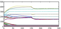
(a) Power allocation

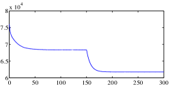
(b) Total cost

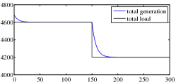
(c) Total mismatch

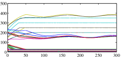
(d) Power allocation

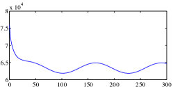
(e) Total cost

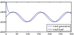
(f) Total mismatch

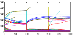
(g) Power allocation

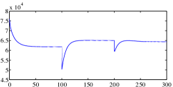
(h) Total cost

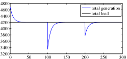
(i) Total mismatch

Figure 1: Evolution of the power allocation, the total cost, and the total mismatch between generation and load under the dac+$\mathsf{L}\partial$ dynamics for the IEEE 118 bus example in different scenarios. In the first case (a)-(c), the communication topology is $\mathcal{G}$, the load is initially $4600$ and later $4200$, and parameters are $\nu_{1}=1$, $\nu_{2}=1.3$, $\alpha=10$, $\beta=40$, and $\epsilon=0.0086$. In the second scenario (d)-(f), the digraph and the parameters remain the same but the load is time-varying given by $P_{l}(t)=4300+100\sin(0.05t)$. In the last case (g)-(i), the parameters remain the same, the communication graph is initially the graph $\hat{\mathcal{G}}$. At $t=100s$, units $\{4,11,25,45\}$ leave the network, resulting in the communication topology $\hat{\mathcal{G}}_{\setminus\{4,11,25,45\}}$, and the remaining agents run the trajectory invariance routine. Later, at $t=200s$, units $\{11,45\}$ join the network while unit $27$ leaves it, resulting in the communication topology $\hat{\mathcal{G}}_{\setminus\{4,25,27\}}$. After implementing the trajectory invariance routine, the dac+$\mathsf{L}\partial$ dynamics eventually converges to an optimizer of the ED problem for the network $\hat{\mathcal{G}}_{\setminus\{4,25,27\}}$.

Next, we consider a time-varying total load given by a constant plus a sinusoid, $P_{l}(t)=4300+100\sin(0.05t)$. With the same communication topology, design parameters, and initial condition as above, Figure 1 (d)-(f) illustrates the behavior of the network under the dac+$\mathsf{L}\partial$ dynamics. As established in Proposition 5.6, the total generation tracks the time-varying load signal and the mismatch between these values has an ultimate bound. Additionally, to illustrate how that the mismatch vanishes if the load becomes constant, we show in Figure 2 a load signal that consists of short bursts of sinusoidal variation that decay exponentially. The difference between generation and load becomes smaller and smaller as the load tends towards a constant signal.

Our final scenario considers addition and deletion of generators. The initial communication topology is the undirected graph $\hat{\mathcal{G}}$ described in Table 1. The design parameters and the initial condition are the same as above. The total load is $4200$ and is same at all times. For the first $100$ seconds, the power allocations converge to a neighborhood of a solution of the ED problem for the set of generators in $\hat{\mathcal{G}}$. At time $t=100s$, the units $\{4,11,25,45\}$ stop generating power and leave the network. We select these generators because of their substantial impact in the total power generation. After this event, the resulting communication graph is $\hat{\mathcal{G}}_{\setminus\{4,11,25,45\}}$, cf. Table 1. The generators implement the trajectory invariance routine, after which the dac+$\mathsf{L}\partial$ dynamics drives the mismatch to zero and minimizes the total cost. At $t_{2}=200s$, another event occurs, the units $\{11,45\}$ get added to the network while the generator $27$ leaves. The resulting communication topology is $\hat{\mathcal{G}}_{\setminus\{4,25,27\}}$, cf. Table 1. After executing the trajectory invariance routine, the dynamics converges eventually to the optimizers of the ED problem for the set of generators in $\hat{\mathcal{G}}_{\setminus\{4,25,27\}}$, as shown in Figure 1(g)-(i). This example illustrates the robustness of the dac+$\mathsf{L}\partial$ dynamics against intermittent generation by the units, as formally established in Proposition 5.7. In addition to the presented examples, we also successfully simulated scenarios of the kind described in Remark 5.4, where the total load is not known to a single generator and is instead the aggregate of the local loads connected to each of the generator buses, but we do not report them here for space reasons.

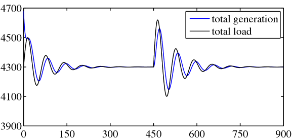
Figure 2: Evolution of the total power generation for the IEEE 118 bus example under the dac+$\mathsf{L}\partial$ dynamics for the communication digraph $\mathcal{G}$, design parameters $\nu_{1}=1$, $\nu_{2}=1.3$, $\alpha=10$, $\beta=40$ and $\epsilon=0.0086$, and time-varying total load. The example depicts the input-to-state stability of the mismatch dynamics.

7 Conclusions

We have designed a novel provably-correct distributed strategy that allows a group of generators to solve the economic dispatch problem starting from any initial power allocation. Our algorithm design combines elements from average consensus to dynamically estimate the mismatch between generation and desired load and ideas from distributed optimization to dynamically allocate the unit generation levels. Our analysis has shown that the mismatch dynamics between total generation and load is input-to-state stable and, as a consequence, the coordination algorithm is robust to initialization errors, time-varying load signals, and intermittent power generation. Our technical approach relies on tools from algebraic graph theory, dynamic average consensus, set-valued dynamical systems, and nonsmooth analysis, including a novel refinement of the LaSalle Invariance Principle for differential inclusions that we have stated and proved. Future work will explore the study of the preservation of the generator box constraints under the proposed coordination strategy, the extension to scenarios that involve additional constraints, such as transmission losses, transmission line capacity constraints, ramp rate limits, prohibited operating zones, and valve-point loading effects, and the study of the stability and convergence properties of algorithm designs that combine our approach here with traditional primary and secondary generator controllers.

Appendix A Refined LaSalle Invariance Principle for differential inclusions

In this section we provide a refinement of the LaSalle Invariance Principle for differential inclusions, see e.g., (Cortés, 2008), by extending the results of (Arsie and Ebenbauer, 2010) for differential equations. Our motivation for developing this refinement comes from the need to provide the necessary tools to tackle the convergence analysis of the coordination algorithms presented in Sections 4 and 5. Nevertheless, the results stated here are of independent interest.

Proposition A.1.

(Refined LaSalle Invariance Principle for differential inclusions): Let $F:{\mathbb{R}}^{n}\rightrightarrows{\mathbb{R}}^{n}$ be upper semicontinuous, taking nonempty, convex, and compact values at every point $x\in{\mathbb{R}}^{n}$. Consider the differential inclusion $\dot{x}\in F(x)$ and let $t\mapsto\varphi(t)$ be a bounded solution whose omega-limit set $\Omega(\varphi)$ is contained in $\SS\subset{\mathbb{R}}^{n}$, a closed embedded submanifold of ${\mathbb{R}}^{n}$. Let $\mathcal{O}$ be an open neighborhood of $\SS$ where a locally Lipschitz, regular function $W:\mathcal{O}\rightarrow{\mathbb{R}}$ is defined. Assume the following holds,

1. the set $\mathcal{E}=\{x\in\SS\;|\;0\in{\mathcal{L}}_{F}W(x)\}$ belongs to a level set of $W$,

2. for any compact set $\mathcal{M}\subset\SS$ with $\mathcal{M}\cap\mathcal{E}=\emptyset$, there exists a compact neighborhood $\mathcal{M}_{c}$ of $\mathcal{M}$ in ${\mathbb{R}}^{n}$ and $\delta<0$ such that $\sup_{x\in\mathcal{M}_{c}}\max{\mathcal{L}}_{F}W(x)\leq\delta$.

Then, $\Omega(\varphi)\subset\mathcal{E}$.

Before proceeding with the proof of the result, we establish an auxiliary result.

Lemma A.2.

Under the hypotheses of Proposition A.1, the sets $\Omega(\varphi)$ and $\mathcal{E}$ have nonempty intersection.

By contradiction, assume $\Omega(\varphi)\cap\mathcal{E}=\emptyset$. Then, using the hypothesis (ii) in Proposition A.1, there exists $\delta<0$ such that $\sup_{x\in\Omega(\varphi)}\max{\mathcal{L}}_{F}W(x)\leq\delta$. Let $x\in\Omega(\varphi)$. Since this set is weakly positively invariant, there exists a trajectory $t\mapsto\tilde{\varphi}(t)$ of the differential inclusion with $\tilde{\varphi}(0)=x$ such that $\tilde{\varphi}(t)\in\Omega(\varphi)$. Since $\frac{d}{dt}W(\tilde{\varphi}(t))\in{\mathcal{L}}_{F}W(\tilde{\varphi}(t))$ for almost all $t\geq 0$, we get $W(\tilde{\varphi}(t))-W(x)\leq\delta t$. This is in contradiction with the fact that $t\mapsto\tilde{\varphi}(t)$ belongs to the compact set $\Omega(\varphi)$, where $W$ is lower bounded. ∎

We are now ready to prove Proposition A.1.

[Proof of Proposition A.1] We consider two cases, depending on whether the set $\Omega(\varphi)$ (a) is or (b) is not contained in a level set of $W$. In case (a), given any $x\in\Omega(\varphi)$, there exists a trajectory of $F$ starting at $x$ that remains in $\Omega(\varphi)$ (because of the weak positive invariance of the omega-limit set). If $x\not\in\mathcal{E}$, then by the hypotheses (ii), there exists a compact neighborhood $\mathcal{M}_{x}$ of $x$ in ${\mathbb{R}}^{n}$ and $\delta<0$ such that $\sup_{y\in\mathcal{M}_{x}}{\mathcal{L}}_{F}W(y)\leq\delta$. Since $\Omega(\varphi)\subset\SS$, the trajectory of $F$ starting at $x$ remains in the set $\mathcal{M}_{x}\cap\SS$ for a finite time, say $t_{1}$. Over the time interval $[0,t_{1}]$, we have $W(t)-W(0)\leq\delta t$. This, however, is in contradiction with the fact that the trajectory belongs to $\Omega(\varphi)$ which is contained in a level set of $W$. Therefore, $x\in\mathcal{E}$, and since this point is generic, we conclude $\Omega(\varphi)\subset\mathcal{E}$.

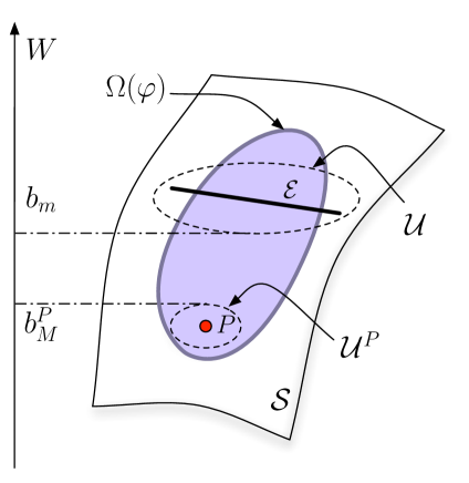
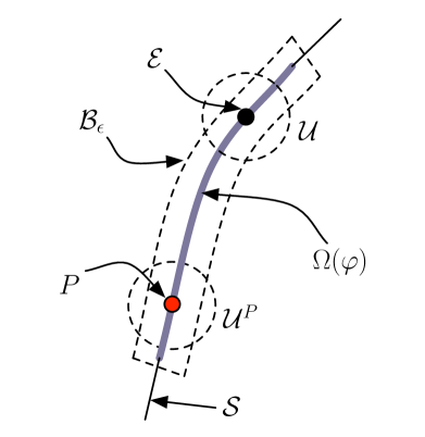
Figure 3: Illustration (adapted from (Arsie and Ebenbauer, 2010, Figure 1)) depicting various elements involved in the case (b) of the proof of Proposition A.1.

Next, we consider case (b) and reason by contradiction, i.e., assume that $\Omega(\varphi)$ is not contained in $\mathcal{E}$ (see Figure 3). Given $\epsilon>0$, let $\mathcal{B}_{\epsilon}\subset\mathcal{O}$ be a compact neighborhood of $\Omega(\varphi)$ in ${\mathbb{R}}^{n}$ such that $d(\mathcal{B}_{\epsilon},\Omega(\varphi))\leq\epsilon$. Let $\mathcal{U}$ be an open neighborhood of $\mathcal{E}$ in ${\mathbb{R}}^{n}$ and define $\mathcal{U}_{\epsilon}=\mathcal{U}\cap\mathcal{B}_{\epsilon}$. Note that $\mathcal{U}_{\epsilon}$ is nonempty because $\Omega(\varphi)\cap\mathcal{E}$ is nonempty by Lemma A.2. Since $\Omega(\varphi)$ is not contained in a level set of $W$ but $\mathcal{E}$ is by hypotheses (i), we can choose $P\in\Omega(\varphi)\setminus\mathcal{E}$ such that $W(P)\not=W(\mathcal{E})$. Without loss of generality, assume $W(P)<W(\mathcal{E})$ (the reasoning is analogous for the other case). Select an open neighborhood $\mathcal{U}^{P}$ of $P$ in ${\mathbb{R}}^{n}$ and define $\mathcal{U}^{P}_{\epsilon}=\mathcal{U}^{P}\cap\mathcal{B}_{\epsilon}$. Define the following quantities

$$b_{m} =\inf_{x\in\mathcal{U}_{\epsilon}}W(x), \quad b^{P}_{M} =\sup_{x\in\mathcal{U}^{P}_{\epsilon}}W(x).$$

Note that the neighborhoods $\mathcal{U}$ and $\mathcal{U}^{P}$ can be chosen such that the set $\Omega(\varphi)\setminus(\mathcal{U}\cup\mathcal{U}^{P})$ is nonempty, compact, and its intersection with $\mathcal{E}$ is empty. Along with this, one can select $\epsilon$ in such a way that $b_{m}>b^{P}_{M}$ and from assumption (ii) we get

$$\sup_{x\in\mathcal{B}_{\epsilon}\setminus(\mathcal{U}\cup\mathcal{U}^{P})}\max{\mathcal{L}}_{F}W(x)\leq\delta<0,$$ (A.28)

(in the case $W(P)>W(\mathcal{E})$, we would reason with the quantities $b_{M}=\sup_{x\in\mathcal{U}_{\epsilon}}W(x)$ and $b_{m}^{P}=\inf_{x\in\mathcal{U}_{\epsilon}^{P}}W(x)$). Since $\Omega(\varphi)$ is the omega-limit set of $\varphi$ and $\mathcal{B}_{\epsilon}$ is a compact neighborhood of $\Omega(\varphi)$, there exists $t_{1}>0$ such that $\varphi(t_{1})\in\mathcal{U}^{P}_{\epsilon}$ and $\varphi(t)\in\mathcal{B}_{\epsilon}$ for all $t\geq t_{1}$. Moreover, since $\Omega(\varphi)\cap\mathcal{E}$ is nonempty, there must also exist $t_{2}>t_{1}$ such that $\varphi(t_{2})\in\mathcal{U}_{\epsilon}$. From continuity of the trajectory we deduce that there exist times $t_{1}^{*},t_{2}^{*}\in(t_{1},t_{2})$, $t_{1}^{*}<t_{2}^{*}$ such that $\varphi(t_{1}^{*})$ and $\varphi(t_{2}^{*})$ lie on the boundary of the compact set $\mathcal{B}_{\epsilon}\setminus(\mathcal{U}_{\epsilon}\cup\mathcal{U}_{\epsilon}^{P})$, with $\varphi(t_{1}^{*})$ belonging to the closure of $\mathcal{U}^{P}_{\epsilon}$ and $\varphi(t_{2}^{*})$ to the closure of $\mathcal{U}_{\epsilon}$. However, this is not possible as $W(\varphi(t_{2}^{*}))\geq b_{m}>b^{P}_{M}\geq W(\varphi(t_{1}^{*}))$ and, in the interval $[t_{1}^{*},t_{2}^{*}]$, the trajectory belongs to $\mathcal{B}_{\epsilon}\setminus(\mathcal{U}_{\epsilon}\cup\mathcal{U}_{\epsilon}^{P})$, where the function $W$ can only decrease due to (A.28), which is a contradiction. ∎

Appendix B Continuity properties of set-valued Lie derivatives

Here we present an auxiliary result for the convergence analysis of the algorithms of Sections 4 and 5.

Lemma A.1.

(Continuity property of set-valued Lie derivatives): Let $W:{\mathbb{R}}^{n}\rightarrow{\mathbb{R}}$ be a locally Lipschitz and regular function. Let $g:{\mathbb{R}}^{n}\times{\mathbb{R}}^{n}\rightarrow{\mathbb{R}}^{n}$ be a continuous function and define the set-valued map $F:{\mathbb{R}}^{n}\rightrightarrows{\mathbb{R}}^{n}$ by $F(x)=\{g(x,\zeta)\;|\;\zeta\in\partial W(x)\}$. Assume that

1. $\SS$ is an embedded submanifold of ${\mathbb{R}}^{n}$ such that $\zeta^{\top}g(x,\zeta)\leq 0$ for all $x\in\SS$ and all $\zeta\in\partial W(x)$,

2. for any $x\in\SS$, if $\zeta^{\top}g(x,\zeta)=0$ for some $\zeta\in\partial W(x)$, then $x\in\mathcal{E}=\{z\in\SS\;|\;0\in{\mathcal{L}}_{F}W(z)\}$.

Then, for any compact set $\mathcal{M}\subset\SS$ with $\mathcal{M}\cap\mathcal{E}=\emptyset$, there exists a compact neighborhood $\mathcal{M}_{c}$ of $\mathcal{M}$ in ${\mathbb{R}}^{n}$ and $\delta<0$ such that $\sup_{x\in\mathcal{M}_{c}}\max{\mathcal{L}}_{F}W(x)\leq\delta$.

We reason by contradiction, i.e., assume that for all compact neighborhoods $\mathcal{M}_{c}$ of $\mathcal{M}$ in ${\mathbb{R}}^{n}$ and all $\delta<0$, we have

$$\sup_{x\in\mathcal{M}_{c}}\max{\mathcal{L}}_{F}W(x)>\delta.$$

Note that this implies that $\sup_{x\in\mathcal{M}_{c}}\max{\mathcal{L}}_{F}W(x)\geq 0$. Now, for each $k\in\mathbb{Z}_{\geq 1}$, consider the compact neighborhood $\mathcal{M}_{k}=\mathcal{M}+\overline{B(0,\frac{1}{k})}$ of $\mathcal{M}$. From the above, we deduce the existence of a sequence $\{x_{k}\}_{k=1}^{\infty}$ with $x_{k}\in\mathcal{M}_{k}$ such that

$$\lim_{k\to\infty}\max{\mathcal{L}}_{F}W(x_{k})=\ell\geq 0.$$ (A.29)

Since the whole sequence belongs to the compact set $\mathcal{M}_{1}$, there exists a subsequence, which we denote with the same indices for simplicity, such that

$$\lim_{k\to\infty}x_{k}=\tilde{x}\in\mathcal{M}.$$ (A.30)

From (A.29), there exists a sequence $\zeta_{k}\in\partial W(x_{k})$ such that

$$\lim_{k\to\infty}\zeta_{k}^{\top}g(x_{k},\zeta_{k})\geq 0.$$ (A.31)

Since $\partial W$ is upper semicontinuous with compact values, the set $\partial W(\mathcal{M}_{1})$ is compact, cf. (Aubin and Cellina, 1984, Proposition 3, p. 42). This implies that the sequence $\{\zeta_{k}\}$ belongs to the compact set $\partial W(\mathcal{M}_{1})$ and so, there exists a subsequence, denoted again by the same indices for simplicity, such that $\zeta_{k}\to\tilde{\zeta}$. Since $\partial W$ is upper semicontinuous and takes closed values, we deduce from (Aubin and Cellina, 1984, Proposition 2, p. 41) that $\tilde{\zeta}\in\partial W(\tilde{x})$. From (A.30) and (A.31), since $g$ is continuous, we obtain $\tilde{\zeta}^{\top}g(\tilde{x},\tilde{\zeta})\geq 0$. By assumption (i), this implies $\tilde{\zeta}^{\top}g(\tilde{x},\tilde{\zeta})=0$. Assumption (ii) then implies $\tilde{x}\in\mathcal{E}$, which along with (A.30) contradicts $\mathcal{M}\cap\mathcal{E}=\emptyset$. ∎

References

- Arsie and Ebenbauer [2010] A. Arsie and C. Ebenbauer. Locating omega-limit sets using height functions. Journal of Differential Equations, 248(10):2458–2469, 2010.
- Aubin and Cellina [1984] J. P. Aubin and A. Cellina. Differential Inclusions, volume 264 of Grundlehren der mathematischen Wissenschaften. Springer, New York, 1984.
- Bacciotti and Ceragioli [1999] A. Bacciotti and F. Ceragioli. Stability and stabilization of discontinuous systems and nonsmooth Lyapunov functions. ESAIM: Control, Optimisation & Calculus of Variations, 4:361–376, 1999.
- Bernstein [2005] D. S. Bernstein. Matrix Mathematics. Princeton University Press, Princeton, NJ, 2005.
- Binetti et al. [2014a] G. Binetti, A. Davoudi, F. L. Lewis, D. Naso, and B. Turchiano. Distributed consensus-based economic dispatch with transmission losses. IEEE Transactions on Power Systems, 29(4):1711–1720, 2014a.
- Binetti et al. [2014b] G. Binetti, A. Davoudi, D. Naso, B. Turchiano, and F. L. Lewis. A distributed auction-based algorithm for the nonconvex economic dispatch problem. IEEE Transaction on Industrial Informatics, 10(2):1124–1132, 2014b.
- Boyd and Vandenberghe [2009] S. Boyd and L. Vandenberghe. Convex Optimization. Cambridge University Press, 2009. ISBN 0521833787.
- Bullo et al. [2009] F. Bullo, J. Cortés, and S. Martínez. Distributed Control of Robotic Networks. Applied Mathematics Series. Princeton University Press, 2009. ISBN 978-0-691-14195-4. Electronically available at http://coordinationbook.info.
- Cherukuri and Cortés [2013] A. Cherukuri and J. Cortés. Distributed generator coordination for initialization and anytime optimization in economic dispatch. IEEE Transactions on Control of Network Systems, 2013. Conditionally accepted. Available at http://carmenere.ucsd.edu/jorge.
- Chowdhury and Rahman [1990] B. H. Chowdhury and S. Rahman. A review of recent advances in economic dispatch. IEEE Transactions on Power Systems, 5(4):1248–1259, November 1990.
- Cortés [2008] J. Cortés. Discontinuous dynamical systems - a tutorial on solutions, nonsmooth analysis, and stability. IEEE Control Systems Magazine, 28(3):36–73, 2008.
- Dominguez-Garcia et al. [2012] A. D. Dominguez-Garcia, S. T. Cady, and C. N. Hadjicostis. Decentralized optimal dispatch of distributed energy resources. In IEEE Conf. on Decision and Control, pages 3688–3693, Hawaii, USA, December 2012.
- Du et al. [2012] L. Du, S. Grijalva, and R. G. Harley. Potential-game theoretical formulation of optimal power flow problems. In IEEE Power and Energy Society General Meeting, San Diego, CA, July 2012. Electronic Proceedings.
- Farhangi [2010] H. Farhangi. The path of the smart grid. IEEE Power and Energy Magazine, 8(1):18–28, 2010.
- Freeman et al. [2006] R. A. Freeman, P. Yang, and K. M. Lynch. Stability and convergence properties of dynamic average consensus estimators. In IEEE Conf. on Decision and Control, pages 398–403, San Diego, CA, 2006.
- [16] IEEE 118 bus. http://motor.ece.iit.edu/data/JEAS_IEEE118.doc.
- Johansson and Johansson [2009] B. Johansson and M. Johansson. Distributed non-smooth resource allocation over a network. In IEEE Conf. on Decision and Control, pages 1678–1683, Shanghai, China, December 2009.
- Kar and Hug [2012] S. Kar and G. Hug. Distributed robust economic dispatch in power systems: A consensus + innovations approach. In IEEE Power and Energy Society General Meeting, San Diego, CA, July 2012. Electronic proceedings.
- Khalil [2002] H. K. Khalil. Nonlinear Systems. Prentice Hall, 3 edition, 2002. ISBN 0130673897.
- Kia et al. [2014] S. S. Kia, J. Cortés, and S. Martínez. Dynamic average consensus under limited control authority and privacy requirements. International Journal on Robust and Nonlinear Control, 2014. To appear.
- Loia and Vaccaro [2013] V. Loia and A. Vaccaro. Decentralized economic dispatch in smart grids by self-organizing dynamic agents. IEEE Transactions on Systems, Man & Cybernetics: Systems, 2013. To appear.
- Mohar [1991] B. Mohar. Eigenvalues, diameter, and mean distance in graphs. Graphs and Combinatorics, 7(1):53–64, 1991.
- Mudumbai et al. [2012] R. Mudumbai, S. Dasgupta, and B. B. Cho. Distributed control for optimal economic dispatch of a network of heterogeneous power generators. IEEE Transactions on Power Systems, 27(4):1750–1760, 2012.
- Pantoja et al. [2014] A. Pantoja, N. Quijano, and K. M. Passino. Dispatch of distributed generators under local-information constraints. In American Control Conference, pages 2682–2687, Portland, OR, June 2014.
- Ren and Beard [2008] W. Ren and R. W. Beard. Distributed Consensus in Multi-Vehicle Cooperative Control. Communications and Control Engineering. Springer, 2008. ISBN 978-1-84800-014-8.
- Simonetto et al. [2012] A. Simonetto, T. Keviczky, and M. Johansson. A regularized saddle-point algorithm for networked optimization with resource allocation constraints. In IEEE Conf. on Decision and Control, pages 7476–7481, Hawaii, USA, December 2012.
- Xiao and Boyd [2006] L. Xiao and S. Boyd. Optimal scaling of a gradient method for distributed resource allocation. Journal of Optimization Theory & Applications, 129(3):469–488, 2006.
- Zhang et al. [2014] W. Zhang, W. Liu, X. Wang, L. Liu, and F. Ferrese. Online optimal generation control based on constrained distributed gradient algorithm. IEEE Transactions on Power Systems, 2014. To appear.
- Zhang and Chow [2012] Z. Zhang and M. Chow. Convergence analysis of the incremental cost consensus algorithm under different communication network topologies. IEEE Transactions on Power Systems, 27(4):1761–1768, 2012.
- Zhang et al. [2011] Z. Zhang, X. Ying, and M. Chow. Decentralizing the economic dispatch problem using a two-level incremental cost consensus algorithm in a smart grid environment. In North American Power Symposium, Boston, MA, August 2011. Electronic Proceedings.