Machine learning for ultrafast X-ray diffraction patterns on large-scale GPU clusters

Abstract.

The classical method of determining the atomic structure of complex molecules by analyzing diffraction patterns is currently undergoing drastic developments. Modern techniques for producing extremely bright and coherent X-ray lasers allow a beam of streaming particles to be intercepted and hit by an ultrashort high energy X-ray beam. Through machine learning methods the data thus collected can be transformed into a three-dimensional volumetric intensity map of the particle itself. The computational complexity associated with this problem is very high such that clusters of data parallel accelerators are required.

We have implemented a distributed and highly efficient algorithm for inversion of large collections of diffraction patterns targeting clusters of hundreds of GPUs. With the expected enormous amount of diffraction data to be produced in the foreseeable future, this is the required scale to approach real time processing of data at the beam site. Using both real and synthetic data we look at the scaling properties of the application and discuss the overall computational viability of this exciting and novel imaging technique.

1. Introduction

X-ray crystallography is currently the most successful method for protein structure determination. A limitation is that this method requires high-quality crystals of the sample protein. This is particularly problematic for membrane proteins which are notoriously hard to crystallize. This class of proteins contains about 20–30% of all proteins and are targeted by 50% of modern drugs; still they comprise less than 0.1% of the known protein structures.

The recent construction of free-electron lasers (FEL) has the potential to revolutionize structural biology by allowing structure determination without the need for crystallization. FEL pulses are intense enough that an interpretable diffraction signal can be recorded from single proteins or viruses. Also, the pulses are short enough to outrun the radiation damage to the particle and the scattered data thus represents the intact particle even though the extreme intensity will destroy the sample within picoseconds.

Since the diffraction data frames are collected one at a time and the extremely intense X-ray pulse destroys the samples, it is impossible to collect multiple exposures of the same particle. However, just like in crystallography, we can use the fact that many biological particles exist in identical copies. Data collected from many identical particles can thus be treated as if they come from the same particle.

In this scheme, particles are injected into the stream of X-ray pulses and intercepted in random orientation [14]. A diffraction pattern represents a curved two-dimensional slice through the modulus of the Fourier transform of the electron density of the particle. Since the particles are assumed identical, the patterns will correspond to different slices through the same Fourier density. If the unknown orientations can be recovered, the diffraction patterns can thus be assembled to the complete three-dimensional Fourier-intensity of the particle.

As opposed to in crystallography, the orientation of each particle is not directly measurable. Instead, the orientations are recovered by maximizing the fit between the individual diffraction patterns. Several algorithms for solving this problem have been proposed [11, 7]. The most successful of these is the Expansion Maximization Compression (EMC) method [11] which has been verified experimentally using artificial samples [12], and which was recently used for the reconstruction of the giant Mimivirus [4].

The LINAC Coherent Light Source (LCLS) [5] has a repetition rate of 120 Hz and a sustained hit-ratio of 20% has been achieved reproducibly. This corresponds to 1 million diffraction patterns in a single 12 hour shift or about 4 TB of data. The European XFEL is becoming operational in 2016 and will have a repetition rate of 27,000 Hz [16].

The 3D-alignment algorithms are computationally very demanding, yet high data volumes are fundamental for achieving high resolution and to balance the low photon signal when studying smaller objects. In the light of the above developments there is an imminent need for a massively parallel implementation of the EMC algorithm to keep up with the increased data rates and the increasing problem size.

Based on previous experience with an implementation for smaller heterogeneous GPU-computers [6], in this paper we present a working fully distributed implementation targeting large-scale clusters of hundreds of GPU computers. In an effort to prepare for the increasing data rates we ensure in our implementation that data can be effectively and flexibly distributed. We also devise a kind of adaptive iteration which allows computational resources to be used in proportion to the resolution of the final reconstruction. Similar techniques, we argue, will be required when handling streaming data at the beam site.

An overview of the XFEL imaging setup and the associated computational methodology is found in §2. Our data parallel and fully distributed implementation is discussed in some detail in §3. Performance results on clusters of up to 100 GPUs, reaching up to and beyond 4 TFLOPS, are presented in §4, and a concluding discussion is found in §5.

2. X-ray laser diffraction and Maximum Likelihood imaging

In this section we summarize the experimental setup and the principles behind 3D imaging with XFELs. The associated data analysis is formulated as a hidden variable Maximum Likelihood problem which can be handled by the Expectation-Maximization algorithm. We also describe the current ‘best practice’ in designing a working such algorithm. Although we certainly expect the methodology to develop further, it seems reasonable to believe that our implementation, or at least a very similar one, will be used extensively when modern XFEL facilities are increasingly being put to use.

2.1. Ultrafast X-ray diffraction patterns

The schematics of collecting data by XFELs is depicted graphically in Figure 2.1. An inflow of samples of biomolecules is intercepted by an X-ray laser pulse resulting in a collection of diffraction images. We denote the raw data output from this procedure by $K=(K_{k})_{k=1}^{M_{\mbox{{\tiny data}}}}$; this is a collection of frames, each containing measured photon counts. The detector is discrete and hence for the $k$th frame, $K_{k}=(K_{ik})_{i=1}^{M_{\mbox{{\tiny pix}}}}$, where $M_{\mbox{{\tiny pix}}}=2^{20}=1024\times 1024$ is a typical resolution. Some pixel counts near the center are missing or may reach saturation as a result of inherent physical limitations with the experimental procedure.

Assuming ideally that the stream of samples consists of identical copies of a single physical object with an electron density $O$, diffraction theory [8] gives that each frame $K_{k}$ is given by a certain slice, an Ewald sphere, of the 3D Fourier transform $W$ of the real space object $O$.

With a sufficiently large collection of frames an estimate $\hat{W}$ of $W$ is first determined. Notably, this estimate lacks information about the Fourier phases since it is based on photon count data only. The final step is therefore a phase retrieval procedure [2, 19], after which an estimate of the real space object can be obtained.

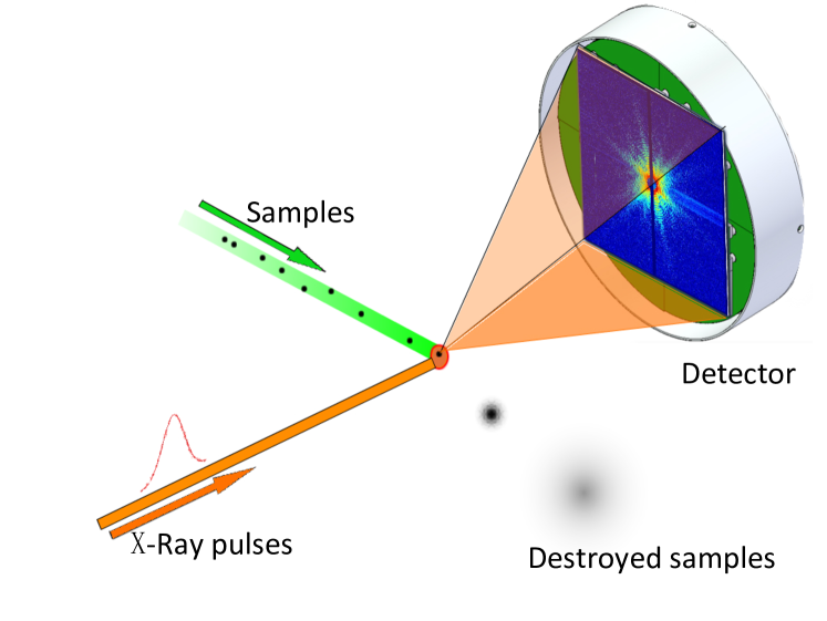
Figure 2.1. The principal setup in X-ray laser imaging. A stream of samples of biomolecules is injected and intercepts with extremely bright and very short pulses of X-ray lasers. While this immediately turns the samples into a plasma, the data collected by the photon count detector comes from a practically undamaged object.

2.2. Maximum Likelihood estimation via Expectation-Maximization

With i.i.d. frames $K=(K_{k})_{k=1}^{M_{\mbox{{\tiny data}}}}$, the Maximum Likelihood estimator is given by

(2.1) $$\hat{W} =\arg_{W}\max\;M_{\mbox{{\tiny data}}}^{-1}\sum_{k=1}^{M_{\mbox{{\tiny data}}}}\log\mathbf{P}(K_{k}|W),$$

that is, for some probabilistic intensity model, maximizing the likelihood of the obtained photon count data when presented with the recorded data. The problem is incomplete for two reasons. Firstly, the true rotation $R_{k}$ of the object in measurement $K_{k}$ is unknown and consequently the frame cannot be directly associated with a definite Ewald sphere. Secondly, the energy of the X-ray pulse, the photon fluence $\phi_{k}$, which hits the sample is also an unknown variable.

Besides the problem of hidden data, the overall signal to noise ratio is very small and implies a grand computational challenge since to counteract this the processed data volume has to be large. With input data corrupted by high noise levels, measures has to be taken in order to design a robust and useful algorithm [18].

The Expectation-Maximization (EM) algorithm [3] aims at producing likelihood estimates with hidden data in a constructive way. The basic procedure of alternating steps of (i) assigning probabilities to the hidden states, and (ii) maximum likelihood estimates of the parameters of the model can be shown under broad conditions to be at least a descent step of the full likelihood [13]. Notably, in step (i) the model parameters are kept fixed, while in (ii) the estimated probabilities of the hidden states (the responsibilities using EM terminology) from step (i) are assumed known.

We now introduce some notation. Firstly, the rotational space is discretized by $(R_{j})_{j=1}^{M_{\mbox{{\tiny rot}}}}$. Since this is generally a non-uniform discretization we denote by $w_{j}$ the prior weight for the $j$th rotation, normalized such that $\sum_{j}w_{j}=1$. In other words, selecting $R_{j}$ with probability $w_{j}$ implies a practically uniform sampling of the rotational space. The intensity space is similarly discretized by the set of points $(q_{i})_{i=1}^{M_{\mbox{{\tiny pix}}}}$ such that using this coordinate system the unknown Fourier intensity at position $R_{j}q_{i}$ can be denoted by $W_{ij}$. Finally, we denote by $\phi_{jk}$ the intensity of the beam that produced data frame $k$, given that the object was rotated according to $R_{j}$.

An early EM algorithm for solving the problem was devised in [11] using the assumption that the signal is Poissonian. This assumption has the benefit of producing an essentially parameter-free algorithm but neglects other potential sources of noise. In practice a Gaussian model has been more successful. More precisely we assume that the measured intensity of the $i$th pixel in the $k$th measurement, when scaled with the photon fluence, is Gaussian around the unknown Fourier intensity $W_{ij}$  [12, 4].

(2.2) $$\log\mathbf{P}(K_{ik}=\kappa|W_{ij},R_{j},\phi_{jk}) \propto-\frac{(\kappa/\phi_{jk}-W_{ij})^{2}}{2\sigma^{2}}=:Q_{ijk}(W,\phi),$$

with $\sigma$ a noise parameter which is kept at conservative values or decreases slightly as the iteration proceeds. Summing over $i$ we get the joint log-likelihood function,

(2.3) $$Q_{jk}(W,\phi):=\sum_{i=1}^{M_{\mbox{{\tiny pix}}}}Q_{ijk}(W,\phi),$$

that is, the logarithm of the probability of observing frame $K_{k}$, given rotation $R_{j}$ and fluence $\phi_{jk}$. Integrating this over the space of rotations we get

$$P_{jk}^{(n+1)} =P_{jk}^{(n+1)}(W^{(n)},\phi^{(n)}):=\mathbf{P}(R_{j}|K_{k},W^{(n)},\phi^{(n)})$$

(2.4) $$=\frac{w_{j}T_{jk}(W^{(n)},\phi^{(n)})}{\sum_{j^{\prime}=1}^{M_{\mbox{{\tiny rot}}}}w_{j^{\prime}}T_{j^{\prime}k}(W^{(n)},\phi^{(n)})},\qquad\mbox{({``E-step''})}$$

in terms of $T_{jk}(W,\phi)\equiv\exp(Q_{jk}(W,\phi))$. Some care is required when evaluating (2.4) to avoid finite precision effects.

Although there is no explicit maximum likelihood formula for computing $(W,\phi)$ given $P$, the following fix-point iteration for the normal equations has been proposed [12],

(2.5) $$W^{(n+1)}_{ij} =\frac{\sum_{k=1}^{M_{\mbox{{\tiny data}}}}P_{jk}^{(n+1)}K_{ik}/\phi_{jk}^{(n)}}{\sum_{k=1}^{M_{\mbox{{\tiny data}}}}P_{jk}^{(n+1)}},$$

(2.6) $$\phi_{jk}^{(n+1)} =\frac{\sum_{i=1}^{M_{\mbox{{\tiny pix}}}}K_{ik}^{2}}{\sum_{i=1}^{M_{\mbox{{\tiny pix}}}}W_{ij}^{(n)}K_{ik}}.\qquad\mbox{({``M-step''})}$$

When the EM-iteration is understood as a descent step of the full likelihood function, this approach of using ‘partial steps’ can be justified [13].

The rotations $(R_{j})_{j=1}^{M_{\mbox{{\tiny rot}}}}$ and the corresponding prior weights $w_{j}$ must be found through some kind of discretization procedure. The suggestion in [11] is to use the fact that quaternions encode rotations; any rotation can be identified as a point on a 4D sphere which can hence be discretized. A suitable geometric object for this purpose is the 600-cell (or hexacosichoron) which is a 4D convex regular 4-polytope whose boundary is composed of 600 tetrahedra. At even larger values of $M_{\mbox{{\tiny rot}}}$ one further uses the fcc-cell in which each tetrahedron is uniformly divided $d$ times into $\{1,4,10,20,35,...\}$ smaller tetrahedra. This implies the relation [11, Appendix C]

(2.7) $$M_{\mbox{{\tiny rot}}}(d) =10\cdot(5d^{3}+d)$$

$$=[6\,300,10\,860,25\,680,50\,100,86\,520]\quad\mbox{for }d=[5,6,8,10,12].$$

In §3.4 below we make an active use of this discretization by increasing $d$ adaptively whenever the increase of likelihood goes below some predefined threshold.

2.3. EM with compression steps: the EMC

A problem with the EM-iteration defined by (2.4) and (2.5)–(2.6) is that averages are computed in discrete space while data is continuous. There are many pairs $(i,j)$ such that $R_{j}q_{i}$ are very close, but in the M-step (2.5) they will be exchanging information with disjoint or nearly disjoint sets of frames. If the end result is to be understood as a continuous object some kind of smoothing procedure has to be devised.

A straightforward way to achieve this is to add expansion/compression-steps. The purpose of the latter step is to compress (average/smooth) the representation into, say, a Cartesian representation with a uniform spatial resolution. The expansion step is the inverse of this operation and takes us back to the working description in $R_{j}q_{i}$-space. The combination of the average (2.5) in the M-step and a compression step then ensures that nearby pixels and rotations have exchanged information with overlapping sets of frames.

Let interpolation weights $f$ and interpolation abscissas $(p_{l})_{l=1}^{M_{\mbox{{\tiny grid}}}}$ be defined such that for $g$ some smooth function,

(2.8) $$g(q) \approx\sum_{l=1}^{M_{\mbox{{\tiny grid}}}}f(p_{l}-q)g(p_{l}).$$

An expansion operator can now be defined,

(2.9) $$W_{ij} =\sum_{l=1}^{M_{\mbox{{\tiny grid}}}}f(p_{l}-R_{j}q_{i})\mathbb{W}_{l},\qquad\mbox{({``e-step''})}$$

which maps values from a grid $\mathbb{W}_{l}:=W(p_{l})$ into the working description $W_{ij}=W(R_{j}q_{i})$. Similarly, a suggestion for the compression operator is given by [11],

(2.10) $$\mathbb{W}_{l} =\frac{\sum_{i=1}^{M_{\mbox{{\tiny pix}}}}\sum_{j=1}^{M_{\mbox{{\tiny rot}}}}f(p_{l}-R_{j}q_{i})W_{ij}}{\sum_{i=1}^{M_{\mbox{{\tiny pix}}}}\sum_{j=1}^{M_{\mbox{{\tiny rot}}}}f(p_{l}-R_{j}q_{i})}.\qquad\mbox{({``c-step''})}$$

It should be noted that, whereas (2.9) is a consistent interpolation, (2.10) rather falls under the framework of Inverse distance weighting. Furthermore, in the implementation discussed here, the M- and the c-steps are intertwined in that the normalization is deferred until after $\mathbb{W}$ has been obtained. Hence we compute (compare (2.5))

(2.11) $$W^{(n+1)}_{ij} =\sum_{k=1}^{M_{\mbox{{\tiny data}}}}P_{jk}^{(n+1)}K_{ik}/\phi_{jk}^{(n)}.$$

The c-step is then computed as

(2.12) $$\mathbb{W}_{l}^{(n+1)} =\frac{\sum_{i=1}^{M_{\mbox{{\tiny pix}}}}\sum_{j=1}^{M_{\mbox{{\tiny rot}}}}f(p_{l}-R_{j}q_{i})W_{ij}^{(n+1)}}{\sum_{i=1}^{M_{\mbox{{\tiny pix}}}}\sum_{j=1}^{M_{\mbox{{\tiny rot}}}}f(p_{l}-R_{j}q_{i})\sum_{k=1}^{M_{\mbox{{\tiny data}}}}P_{jk}^{(n+1)}}.$$

In Algorithm 1 a summary of the algorithm which will be considered here is given. As we shall next see, the algorithm has a distinct data parallel character and can be distributed efficiently.

Input: Initial guess of the 3D intensity distribution $\mathbb{W}^{(0)}$ of the object on the grid $(p_{l})_{l=1}^{M_{\mbox{{\tiny grid}}}}$, and an initial estimate of the rotational probabilities $P^{(0)}$.

Output: Improved image $\mathbb{W}$ and probabilities $P$.

1:repeat

2:     $n=0,1,\ldots$

3:     $W^{(n)}:=e\circ\mathbb{W}^{(n)}$. {Expansion step, (2.9).}

4:     $P^{(n+1)}:=E\circ P^{(n)}$. {Expectation step, (2.4).}

5:     $[W^{(n+1)},\mathbb{W}^{(n+1)}]:=cM\circ W^{(n)}$. {Combined Maximization and compression, (2.11) and (2.12).}

6:until change in either $\mathbb{W}$ or likelihood is small enough

Algorithm 1 The EMC algorithm.

3. Parallelization in GPU clusters

By inspection the algorithm under consideration is computationally intensive as it is composed mainly of blocks of nonlinear matrix operations. This implies that it can be expected to perform well on modern data parallel accelerators in general and on GPUs in particular. The most common approach to distributed GPU computing is to transfer data via an MPI-layer and use CUDA at the computational nodes. This master-slave approach has been employed successfully in other multi-GPU applications [10, 15], and is also our approach.

In this section we take a bottom-up approach and first discuss the single-node data parallelism and then extend the same scheme to a distributed environment. We next devise a fully distributed approach in which very large diffraction datasets may be considered, and we finally also develop a simple but efficient multiresolution type adaptivity.

3.1. Single-node data parallelism

In an implementation targeting a single GPU-node, data must be shared between the cores of the GPU. Currently, the typical resolution is to reconstruct a $64\times 64\times 64$ or a $128\times 128\times 128$ intensity model using about 1000 diffraction patterns (see Table 4.1). Given the complexity of the steps of the algorithm, the E-step (2.4) stands out as the most expensive part. Recall that the E-step estimates likelihoods $P_{jk}$ for rotations $R_{j}$ given data frames $K_{k}$, and it therefore makes sense to distribute the resulting probability matrix $P$. With a usually quite large rotational space, the algorithm requires around 1.5 GB of memory to store the $M_{\mbox{{\tiny data}}}\times M_{\mbox{{\tiny rot}}}$ matrix $P$ even for a low resolution reconstruction. Such a matrix can be distributed by dividing the rotational space or by distributing the images themselves. In the single-node implementation we choose not to distribute by images since $M_{\mbox{{\tiny data}}}$ is usually much smaller than $M_{\mbox{{\tiny rot}}}$.

Our single-node EMC was implemented using CUDA with C/C++ wrappers and the implementation closely follows the logic in Algorithm 1. Briefly, the CPU controls the overall procedure and streams all required data to the GPU as well as writes the output. Hence the diffraction patterns are initially loaded and copied into GPU memory. In each EMC iteration, the compute intensive steps (2.9), (2.4), (2.11) and (2.12) are all evaluated on the GPU.

To discuss those steps, let a ‘chunk’ $C_{c}$ denote a contiguous set of rotations, writing $R^{c}=\{R_{j};\;j\in C_{c}\}$, $C_{c}:=\{j;\;j_{-}^{c}\leq j<j_{+}^{c}\}$. Let the number of rotations in the set $C_{c}$ be denoted by $|C_{c}|$, and the total number of chunks as indexed by $c$ by $M_{\mbox{{\tiny chunks}}}$. The computations in the e-step (2.9) and the M-step (2.11) are partitioned into chunks naturally. Neither of those steps involve a normalization over the rotational space, and therefore we can easily calculate and update partial slices $W^{c}_{ij}$ in a GPU kernel. Each kernel uses $|C_{c}|$ blocks, and each block takes care of the computations for one rotation.

The E-step (2.4) and the c-step (2.12) are more complex due to the normalization over the rotational space. For the latter kernel $M_{\mbox{{\tiny data}}}\times|C_{c}|$ blocks are used and each thread in the block calculates one value of the nominator in (2.4). The normalization is then performed in a separate final sweep. In the c-step the updated model is determined by averaging among chunks, rotations, and diffraction patterns. Here the numerator and denominator in (2.12) are calculated separately with the division as a final step. The associated GPU kernel uses $|C_{c}|$ blocks, and each block handles one slice in $R^{c}$.

3.2. Distributed implementation on a GPU cluster

As argued previously, partitioning the rotational space implies that the algorithm fits efficiently into memory. This scheme is also simple enough to be extended to GPU clusters under our preferred master-slave approach. Additionally, our distributed EMC algorithm has the feature of not only dividing the computations of the most expensive step (the E-step, see Figure 4.2), but also that it localizes the computations of the corresponding photon fluence $\phi$, which is the second most expensive step.

In the implementation, we associate each GPU with one CPU at the same cluster node, hence uses one MPI process per GPU, and we designate one such CPU/GPU pair as the master node. For every EMC iteration, each pair takes care of local computations and synchronizes when necessary. The master CPU has the overall control of how EMC synchronizes over the nodes, and each CPU is in charge of the local GPU computations. Communications between the nodes are thus only needed in 3 places. Firstly, diffraction patterns and algorithmic configurations must be broadcast before the algorithm starts. Secondly, for each chunk $C_{c}$, local estimated probabilities $P^{c}$ must be normalized globally over all nodes. Thirdly and finally, the local model $\mathbb{W}^{c}$ must be merged (averaged) at the end of each iteration. The data flow among the nodes in our implementation is shown in Figure 3.1. This procedure is a special case of the fully distributed EMC, which we now proceed to discuss.

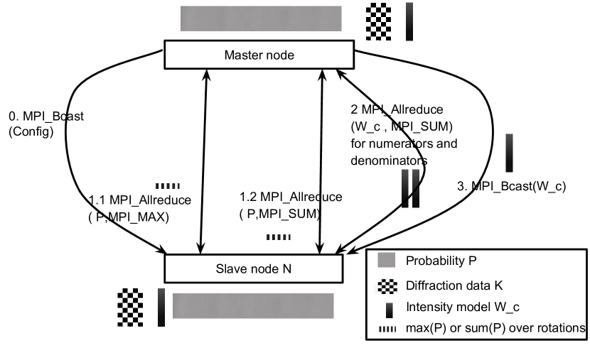
Figure 3.1. Communication pattern between the nodes for the distributed EMC implementation. The rectangles representing data have the correct scale with respect to the variable they represent (this is the small case of Table 4.1). Step 0 is the initialization phase, where only configuration is broadcast, and diffraction patterns $K$ and initial model W_c are fetched by each node. For each EMC iteration, intensity updates are performed via steps 1 through 3 among the GPU nodes. W_c in the figure is the intensity model $\mathbb{W}$.

3.3. Fully distributed EMC

For large enough datasets, the diffraction patterns themselves also need to be distributed as they no longer fit on a single node. The chunks $C_{c}$ are now sets of two-dimensional indices, $C_{c}:=\{(j,k);\;k_{-}\leq k<k_{+},j_{-}\leq j<j_{+}\}$. With this Cartesian grid-like topology, data is either communicated over the rotational space (along the $j$-direction), or over image space (along the $k$-direction).

The steps that do not involve the diffraction patterns in a global sense, namely the E-step (2.4) and the fluence calculation of the M-step (2.6), are not affected by this novel way of partitioning data, and can therefore be implemented as previously described. The remaining steps (2.11)–(2.12) require data to be broadcast in the $k$-direction. The resulting data flow among the nodes in our implementation is implicitly shown in Figure 3.2. Step 1.1 and 1.2 in Figure 3.2 are only necessary for GPUs that share the same Cartesian column in $K$, while steps 0, 2, and 3 are global communications. Further details of the fully distributed EMC are listed in Algorithm 2. Note that, in both distributed EMC implementations, diffraction patterns $K$ and the initial model $\mathbb{W}^{0}$ are pulled by each node according to the data configuration.

Input: Diffraction patterns $K$, initial guess of the 3D intensity distribution $\mathbb{W}^{(0)}$.

Distribute: Divide all computational nodes into a Cartesian grid. Distribute diffraction patterns $K$ along the $k$-direction, and probabilities $P$ along the $j$-direction.

1:repeat

2:     At each node copy local data from CPU to GPU;

3:     Execute expansion step (2.9): at each GPU and for each partition $c$, expand $\mathbb{W}^{(n)}$ into $W_{ij}^{c}$, using the GPU kernel $\mathbf{\_\_global\_\_}\mathbf{void}\text{ expansion }\texttt{<<<}|C_{c}|,256\texttt{>>>}$;

4:     Execute expectation step (2.4): compute the probabilities $P$ as in (2.4) (steps 1.1 and 1.2 in Figure 3.2). The GPU kernel is $\mathbf{\_\_global\_\_}\mathbf{void}\text{ calculate\_probability}\texttt{<<<}M_{\mbox{{\tiny data}}}\times|C_{c}|,256\texttt{>>>}$. Normalization is performed among nodes that share the same distribution of $K$, hence a $\mathbf{MPI\_AllReduce}$ operation in the $j$-direction.

5:     Execute the maximization step (2.11): update $W_{ij}^{c}$ using the GPU kernel $\mathbf{\_\_global\_\_}\mathbf{void}\text{ update\_slices}\texttt{<<<}|C_{c}|,256\texttt{>>>}$;

6:     Execute the compression step (2.12): update $\mathbb{W}$ according to (2.12), the numerators and denominators are calculated via the GPU kernel $\mathbf{\_\_global\_\_}\mathbf{void}\text{ insert\_slices}\texttt{<<<}|C_{c}|,256\texttt{>>>}$; For all nodes, use $\mathbf{MPI\_AllReduce}$ to transfer and add the numerators and denominators separately, and then perform the final division by the GPU kernel $\mathbf{\_\_global\_\_}\mathbf{void}\text{ insert\_slices\_division}\texttt{<<<}\lceil\frac{M_{\mbox{{\tiny rot}}}}{256}\rceil,256\texttt{>>>}$; Finally determine $\mathbb{W}^{n+1}$ in the c-step as in (2.12) (step 2 in Figure 3.2).

7:     Use $\mathbf{MPI\_Bcast}$ to update $\mathbb{W}^{n+1}$ for every node (step 3 in Figure 3.2).

8:until change in either $\mathbb{W}$ or likelihood is small enough

Algorithm 2 Fully distributed data-parallel version of the EMC algorithm.

Figure 3.2. Communication pattern of the fully distributed EMC implementation. A node group is a set of GPU/CPU pairs which share the same partition of diffraction data $K$. Communications among node groups are illustrated by thin arrows, and communications within a node group are shown in wide arrows. The master node works as a normal node in node group 1 with the exception for steps 0 and 3. According to the notation in the figure, W_c is the intensity model $\mathbb{W}$. After the configuration is broadcast, every node fetches their own portion of $K$, and the same initial model $\mathbb{W}$.

The data transfers, in both the distributed EMC and in the fully distributed EMC implementation, can be implemented efficiently. Firstly, the diffraction patterns are fetched by each node in the initial phase. Secondly, when normalizing the probability, only maximal rotational probabilities and sums are necessary, and we may use $\mathbf{MPI\_AllReduce}$. Thirdly, for the fully distributed EMC, the use of a Cartesian communicator streamlines the communications.

3.4. Adaptive EMC

Previously, we aimed for an efficient execution by distributing data and using an increasing number of compute nodes. In most actual experience with the method a fairly highly resolved rotational space is used and one typically observes a likelihood which slowly but steadily improves. The performance critical steps of the method, the E-step (2.4) and part of the combined M/c-step (2.12), scale directly with the discretization of the rotational space $M_{\mbox{{\tiny rot}}}$. Hence it seems reasonable not to waste computational time using a large value of $M_{\mbox{{\tiny rot}}}$ before the likelihood has improved sufficiently. A simple way to achieve this is to start using some small value of $M_{\mbox{{\tiny rot}}}$, $M_{\mbox{{\tiny rot}}}(d_{0})$ say, and increase $d$ in (2.7) whenever the current value seems too small to improve the likelihood any further. In practice we increase $d$ by 1 when

(3.1) $$\left\lvert L^{n}-L^{n-1}\right\rvert\leq 0.01\left\lvert L^{n}\right\rvert,$$

with $L^{n}$ the likelihood at iteration $n$.

4. Experiments

We now proceed to investigate the achievable performance of our implementation. Our datasets are either real ones and of similar quality to those currently being processed, or are synthetic and of considerably larger size to be able to assess future performance profiles. In particular, we will explore the possibility to obtain a highly resolved image from a very large diffraction dataset on a cluster consisting of 100 GPUs.

4.1. Setup and basic profiling

We ran our experiments using a 32-node homogeneous GPU cluster. Each node of the cluster is equipped with 4 six-core Intel Xeon E5-2620 CPUs and 4 Nvidia GeForce GTX 680 GPUs. All the CPU cores operate at 2.0 GHz with 32K L1i and L1d catches. They are organized as 2 NUMA nodes with a total of 64 GB memory. Each GTX 680 GPU has 4GB memory, and the reported nominal peak performance in single precision of matrix multiplication, matrix left division, and the Fast Fourier Transform are $[966,573,101]$ GFLOPS, respectively [9]. Cluster nodes are interconnected using a QDR Infiniband with a bandwidth of 32 Gbit/s. We measured the bandwidth of CPU/GPU connections by doing a host-to-device and device-to-host memory copy, and we found that the bandwidth in both direction is around 3 GB/s. For the compilers and libraries, we used GCC 4.4.6, CUDA 5.0, and Open MPI 1.5.4. By considering the inter-node MPI bandwidth, the intra-node CPU/GPU bandwidth and the data volume which needs to be transferred, we judge that our implementation is not bandwidth bound.

We used mainly two different diffraction datasets. A smaller case consisting of 198 images from an X-ray diffraction experiment with the giant Mimivirus [4, 17] performed at the Linac Coherent Light Source (LCLS). A larger case was obtained through synthetic simulation for an icosahedral shape and consists of 1000 frames. Figure 4.1 displays samples of these diffraction patterns.

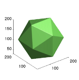
(a)

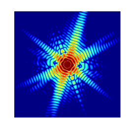
(b)

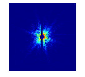
(c)

Figure 4.1. Left: real-space icosahedron, middle: resulting synthetic diffraction pattern, right: X-ray diffraction pattern from the Mimivirus. The two diffraction patterns are plotted in logarithmic scale.

In Table 4.1 we list the sizes of all relevant data in our experiments. The experiments were configured to reconstruct a small ($64\times 64\times 64$), or, respectively, a large ($128\times 128\times 128$) 3D intensity model in single precision. In §4.2 we also ran a ‘giant’ case consisting of our synthetic dataset, but duplicated ten times (i.e. a total of 10,000 frames).

Set $\#$	data	$M_{\mbox{{\tiny data}}}$	$M_{\mbox{{\tiny pix}}}$
1	Mimivirus	198	4096
2	Mimivirus	198	16384
3	synthetic	1000	4096
4	synthetic	1000	16384
5	synthetic	10000	4096
6	synthetic	10000	16384

Table 4.1. Sizes of the different datasets used in our experiments. Note that the value of $M_{\mbox{{\tiny pix}}}$ is the result after binning the raw data $1024\times 1024$ into a coarser $64\times 64$ (or $128\times 128$) format, and note also the relation $M_{\mbox{{\tiny grid}}}=M_{\mbox{{\tiny pix}}}^{3/2}$. In all these experiments we used the value $M_{\mbox{{\tiny rot}}}=86520$.

The result of profiling our single-GPU implementation provided a motivation for our approach to distribute data in our multi-GPU implementation. We profiled the single-GPU implementation by reconstructing at low resolution the Mimivirus dataset (Set #1 in Table 4.1) on one Nvidia GeForce GTX 680. Figure 4.2 displays the computational statistics after averaging over the first 10 iterations. As expected, the E-step was the most expensive step, consuming more than 55% of the total time. This means that it is preferable to distribute data along the rotational space (along the $j$-direction), at least given this relatively small number of diffraction patterns. Since the probability $P_{jk}$ has the same size as the photon fluence $\phi_{jk}$, this also means that the second most expensive step, i.e. the computation of $\phi$, parallelizes very well.

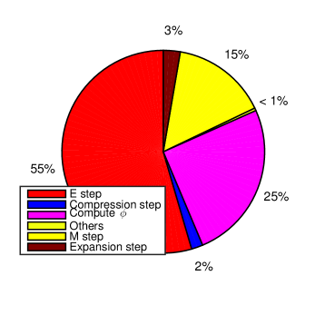
Figure 4.2. Profiling the single GPU EMC implementation. The two most expensive operations are the E-step (2.4) and updating the photon fluence (2.6).

4.2. Performance analysis

In this section we report results from our distributed EMC from §3.2 for both the Mimivirus dataset and the synthetic dataset on up to 32 GPUs. We also look at the performance of the fully distributed EMC from §3.3 using the ‘giant’ synthetic dataset, consisting of 10,000 diffraction patterns. In contrast to these large-scale experiments, we will also explore the performance of adaptive EMC on a single GPU.

We first ran some experiments with the distributed EMC implementation as discussed in §3.2. We measured Amdahl’s efficiency,

(4.1) $$E=\dfrac{T(1)}{nT(n)}=\dfrac{T(1)}{T(1)(B+\frac{1}{n}(1-B))}=\dfrac{1}{nB+(1-B)},$$

where $n$ is the number of GPUs, and $B$ the fraction of the algorithm that is serial. The results are shown in Figure 4.3. As can be seen we obtain a nearly perfect efficiency, at least up to 32 GPUs.

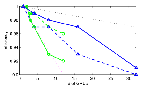
Figure 4.3. Measured efficiencies for dataset #1–4. Circles: real Mimivirus data, triangles: synthetic dataset, solid: $M_{\mbox{{\tiny pix}}}=16384$, dashed: $M_{\mbox{{\tiny pix}}}=4096$. Upper dotted line: Amdahl’s efficiency (4.1) with $B=0.001$, lower dotted line: $B=0.01$.

We next ran some really large-scale experiments for the fully distributed EMC implementation. In an attempt to follow the topology of our cluster, we distributed the rotational space (i.e. the $j$-direction) over a total of 25 nodes, and for the 4 GPUs belonging to the same node, we distributed the 10,000 diffraction patterns uniformly.

Defining one multiplication as 1 FLOP and one division as 8 FLOPs, we find by inspection that one EMC iteration requires about $M_{\mbox{{\tiny rot}}}\times M_{\mbox{{\tiny data}}}\times M_{\mbox{{\tiny pix}}}\times 27\times 10^{-9}$ GFLOPs. Table 4.2 lists the average execution time per iteration and the achieved GFLOPS per GPU. It is remarkable that we loose less than 4% floating point performance at 100 GPUs compared to 16 GPUs. In fact, the fully distributed EMC implementation achieves a higher floating point performance when compared to the single GPU implementation (32.9 GFLOPS and 39.4 GFLOPS, respectively, for $M_{\mbox{{\tiny pix}}}=4096$ and $M_{\mbox{{\tiny pix}}}=16384$). Indeed, these figures compare favorably with the online GPU benchmark [9], where square matrix-matrix multiplication in single precision achieves $[4.4,32.6,181]$ GFLOPS, respectively, at the comparable matrix sizes $N=[16384,65536,262144]$.

	$M_{\mbox{{\tiny pix}}}=4096$		$M_{\mbox{{\tiny pix}}}=16384$
# GPUs	Time (s)	GFLOPS/GPU	Time (s)	GFLOPS/GPU
16	164.6	$36.3$	552.2	$43.3$
32	83.5	$35.8$	281.2	$42.5$
64	42.3	$35.3$	141.6	$42.3$
96	28.3	$35.2$	95.4	$41.8$
100	27.2	$35.2$	91.6	$41.8$

Table 4.2. Average execution time and floating point performance per GPU and per iteration using the fully distributed EMC.

Finally, we also performed some experiments with our adaptive EMC algorithm. For simplicity we used a single GPU only, and we reconstructed a small $64\times 64\times 64$ intensity model. For the adaptivity we increased $d$ in (2.7) from 5 to 12 according to the likelihood-based criterion (3.1). Figure 4.4 displays the relative difference of likelihood together with the execution time per iteration. As expected, the execution time increases as the resolution of the rotational space increases. Whenever $d$ is increased, there is a sharp peak in the relative likelihood difference, indicating iterations that successfully increase the likelihood. The performance gain for the adaptive version is quite remarkable, $7341.6$ seconds compared to $14524$ seconds for the original version, using 60 iterations for both runs. By the very simplicity of this approach, we expect that this gain of a factor of about 2 remains also for larger load cases.

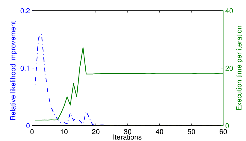
Figure 4.4. Difference of likelihood (3.1) and the corresponding execution time (in seconds) for the first 60 iterations.

4.3. Scalability

Instead of a scaling for a fixed problem-size, we study a metric of scalability that takes the data volume into account. Define the effective problem size as $V(C)\equiv M_{\mbox{{\tiny rot}}}(C)\times M_{\mbox{{\tiny pix}}}(C)\times M_{\mbox{{\tiny data}}}(C)$ for $C$ a problem configuration. For two different such configurations $C_{1}$ and $C_{2}$, the scalability $S(C_{1},C_{2})$ is then defined as

(4.2) $$S(C_{1},C_{2}) =\dfrac{T(C1)/T(C2)}{V(C_{1})/V(C_{2})},$$

where $T(C)$ is the execution time for configuration $C$. A superlinear scalability $S(C_{1},C_{2})<1$ means that the program works more efficiently with configuration $C_{2}$, and also suggests that the program does not make full use of the computing power in $C_{1}$. The situation $S(C_{1},C_{2})>1$ may happen for a problem which is compute-bound.

Figure 4.5 displays the scalabilities of different configurations. Notably, the cases $S(2,1)$ and $S(4,3)$ show superlinear scalability. Since only $M_{\mbox{{\tiny pix}}}$ is changed in both cases, we judge that this is an effect of that the GPU kernels of the c- and e-step are not fully loaded. To the contrary, increasing $M_{\mbox{{\tiny data}}}$ makes the scalabilities $S(3,1)$ and $S(4,2)$ larger than 1. For the latter case we see that as we add more GPUs, we obtain a slightly better scalability. This indicates that as the size of the datasets increases, the fully distributed EMC becomes a favorable choice.

Finally, with $S(4,1)$, we compare a synthetic dataset to a real one, and we simultaneously increase $M_{\mbox{{\tiny pix}}}$ and $M_{\mbox{{\tiny data}}}$. However, the values in this group only slightly differ from eg. $S(4,2)$, which suggests that $M_{\mbox{{\tiny data}}}$ plays a more prominent role than $M_{\mbox{{\tiny pix}}}$ when measuring performance.

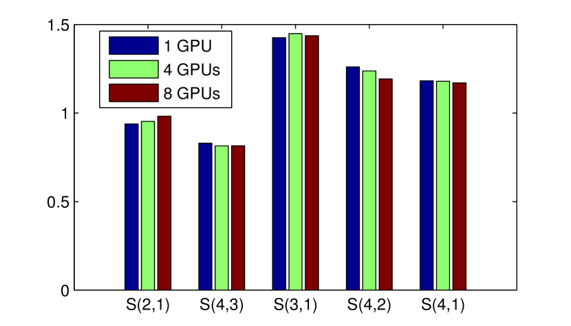
Figure 4.5. The scalability $S(C_{1},C_{2})$ of configuration $C_{1}$ and $C_{2}$, according to (4.2), with $C_{1}$ and $C_{2}$ chosen among cases 1–4 in Table 4.1.

5. Conclusions

We have implemented the EMC algorithm for the assembly of randomly oriented diffraction patterns on GPUs using the CUDA framework and have extended the algorithm to run efficiently on multiple GPUs. We use two different partition schemes depending on the number of diffraction patterns. For a medium-sized dataset we partition the rotational space only, while for a large amount of data we also distribute the images themselves. We observe almost linear speedups for up to 100 GPUs and a parallel efficiency that thus compares very well with other MPI/CUDA applications [10, 20, 21]. We also devised an adaptive technique by which the resolution is increased on par with the increase in likelihood. In our experiments this idea worked very well and we expect similar ideas to be useful in implementations on site where data is processed in a streaming fashion [1].

It seems likely that our implementation is going to develop and adapt further as larger datasets become available. Hopefully, the present software framework can substantially shorten the development cycle for novel algorithms targeting large and noisy datasets.

Hit-ratios and data quality at the LCLS is steadily improving and in 2016 the European XFEL will become operational and provide a repetition rate of 27,000 Hz, a 200-fold increase compared to the LCLS. With this, data analysis will become a bottleneck and EMC in particular is the main computational step in this analysis. With this work we hope to ensure that data analysis can keep up with the rapid development of X-ray laser facilities, while simultaneously enabling the study of biological particles from single proteins to viruses.

References

- Andreasson et al. [2014] J. Andreasson et al. Automated identification and classification of single particle serial femtosecond X-ray diffraction data. Opt. Express, 22(3):2497–2510, 2014. doi:10.1364/OE.22.002497.
- Chapman et al. [2006] H. N. Chapman et al. High-resolution ab initio three-dimensional x-ray diffraction microscopy. J. Opt. Soc. Am. A, 23(5):1179–1200, 2006. doi:10.1364/JOSAA.23.001179.
- Dempster et al. [1977] A. P. Dempster, N. M. Laird, and D. B. Rubin. Maximum likelihood from incomplete data via the EM algorithm. J. R. Stat. Soc. Ser. B Stat. Methodol., 39:1–38, 1977.
- Ekeberg [2012] T. Ekeberg. Flash Diffractive Imaging in Three Dimensions. PhD thesis, Uppsala university, 2012.
- Emma et al. [2010] P. Emma et al. First lasing and operation of an Ångström-wavelength free-electron laser. Nature Photon., 4(9):641–647, 2010. doi:10.1038/nphoton.2010.176.
- Engblom and Liu [2014] S. Engblom and J. Liu. X-ray laser imaging of biomolecules using multiple GPUs. In R. Wyrzykowski, J. Dongarra, K. Karczewski, and J. Waśniewski, editors, Parallel Processing and Applied Mathematics, Lecture Notes in Computer Science, pages 480–489. Springer, Berlin, 2014. doi:10.1007/978-3-642-55224-3_45.
- Fung et al. [2008] R. Fung, V. Shneerson, D. K. Saldin, and A. Ourmazd. Structure from fleeting illumination of faint spinning objects in flight. Nature Phys., 5(1):64–67, 2008. doi:10.1038/nphys1129.
- Gaffney and Chapman [2007] K. J. Gaffney and H. N. Chapman. Imaging atomic structure and dynamics with ultrafast X-ray scattering. Science, 316(5830):1444–1448, 2007. doi:10.1126/science.1135923.
- [9] GPU Bench. GPU comparison report: Quadro K5000, 2012. URL http://folk.uio.no/jorgentr/GPUBenchReport. Accessed: 2014-04-11.
- Jacobsen et al. [2010] D. A. Jacobsen, J. C. Thibault, and I. Senocak. An MPI-CUDA implementation for massively parallel incompressible flow computations on multi-GPU clusters. In 48th AIAA Aerospace Sciences Meeting and Exhibit, volume 16, 2010. doi:10.2514/6.2010-522.
- Loh and Elser [2009] N. D. Loh and V. Elser. Reconstruction algorithm for single-particle diffraction imaging experiments. Phys. Rev. E, 80(2):026705, 2009. doi:10.1103/PhysRevE.80.026705.
- Loh et al. [2010] N. D. Loh et al. Cryptotomography: Reconstructing 3D Fourier intensities from randomly oriented single-shot diffraction patterns. Phys. Rev. Lett., 104:225501, 2010. doi:10.1103/PhysRevLett.104.225501.
- Neal and Hinton [1998] R. M. Neal and G. E. Hinton. A view of the EM algorithm that justifies incremental, sparse, and other variants. In Learning in Graphical Models, pages 355–368. Kluwer, 1998.
- Neutze et al. [2000] R. Neutze, R. Wouts, D. van der Spoel, and J. Hajdu. Potential for biomolecular imaging with femtosecond X-ray pulses. Nature, 406(6797):752–757, 2000. doi:10.1038/35021099.
- Pennycook et al. [2011] S. J. Pennycook, S. D. Hammond, S. A. Jarvis, and G. R. Mudalige. Performance analysis of a hybrid MPI/CUDA implementation of the NASLU benchmark. ACM SIGMETRICS Perf. Eval. Rev., 38(4):23–29, 2011. doi:10.1145/1964218.1964223.
- Schneidmiller and Yurkov [2011] E. A. Schneidmiller and M. V. Yurkov. Photon beam properties at the European XFEL, 2011. December 2010 Revision.
- Seibert et al. [2011] M. M. Seibert et al. Single mimivirus particles intercepted and imaged with an X-ray laser. Nature, 470(7332):78–81, 2011. doi:10.1038/nature09748.
- Serkez et al. [2014] S. Serkez, V. Kocharyan, E. Saldin, I. Zagorodnov, G. Geloni, and O. Yefanov. Perspectives of imaging of single protein molecules with the present design of the European XFEL: part I - X-ray source, beamlime optics and instrument simulations, 2014. Available at http://arxiv.org/abs/1407.8450.
- Shapiro et al. [2005] D. Shapiro et al. Biological imaging by soft x-ray diffraction microscopy. Proc. Natl. Acad. Sci. USA, 102(43):15343–15346, 2005. doi:10.1073/pnas.0503305102.
- Wang et al. [2013] Y. Wang, Y. Dou, S. Guo, Y. Lei, and D. Zou. CPU–GPU hybrid parallel strategy for cosmological simulations. Concurrency Computat.: Pract. Exper., 2013. doi:10.1002/cpe.3046.
- Zaspel and Griebel [2013] P. Zaspel and M. Griebel. Solving incompressible two-phase flows on multi-GPU clusters. Comput. & Fluids, 80:356–364, 2013. doi:10.1016/j.compfluid.2012.01.021.