Scaling properties of a complete X-ray selected galaxy group sample

Abstract

Context. Upcoming X-ray surveys like eROSITA require precise calibration between X-ray observables and mass down to the low-mass regime to set tight constraints on the fundamental cosmological parameters. Since an individual mass measurement is only possible for relatively few objects, it is crucial to have reliable and well understood scaling relations that relate the total mass to easily observable quantities.

Aims. The main goal of this work is to constrain the galaxy group scaling relations corrected for selection effects, and to quantify the influence of non-gravitational physics at the low-mass regime.

Methods. We analyzed XMM-Newton observations for a complete sample of galaxy groups selected from the ROSAT All-Sky Survey and compared the derived scaling properties with a galaxy cluster sample. To investigate the role played by the different non-gravitational processes we then compared the observational data with the predictions of hydrodynamical simulations.

Results. After applying the correction for selection effects (e.g., Malmquist bias), the $L_{\text{X}}$-$M$ relation is steeper than the observed one. Its slope (1.66$\pm$0.22) is also steeper than the value obtained by using the more massive systems of the HIFLUGCS sample. This behavior can be explained by a gradual change of the true $L_{\text{X}}$-$M$ relation, which should be taken into account when converting the observational parameters into masses. The other observed scaling relations (not corrected for selection biases) do not show any break, although the comparison with the simulations suggests that feedback processes play an important role in the formation and evolution of galaxy groups. Thanks to our master sample of 82 objects spanning two order of magnitude in mass, we tightly constrain the dependence of the gas mass fraction on the total mass, finding a difference of almost a factor of two between groups and clusters. We also found that the use of different AtomDB versions in the calculation of the group properties (e.g., temperature and density) yields a gas fraction of up to 20$\%$ lower than an older version.

1 Introduction

Groups and clusters of galaxies are the largest virialized structures in the Universe. They form by continuous accretion of smaller mass units such as field galaxies, groups, and small clusters. As a consequence of this accretion, the mass function of virialized systems is quite steep, and thereby, low-mass systems (often referred to as groups) are more common than rich clusters. Differently from massive clusters, the impact of non-gravitational processes (cooling, AGN feedback, star formation, and galactic winds) in galaxy groups begins to prevail over the gravity because of their shallower potential well. These factors make galaxy groups great laboratories through which to understand the complex baryonic physics involved. Even though they play a central role in the process of structure formation and evolution, they have been studied less frequently than massive clusters. Only recently, thanks to the high sensitivity and resolution of X-ray observatories such as XMM-Newton, Chandra, and Suzaku, the gas content of groups has been studied in more detail. Although several works indicate that groups are consistent with being scaled-down clusters (e.g., Osmond & Ponman 2004; Sun et al. 2009), many independent investigations conducted during the past decade have found that at low masses some scaling relations (e.g., $L_{\text{X}}$-$M$ and entropy-$T$) deviate from the relations of the most massive systems (e.g., Sun et al. 2009; Eckmiller et al. 2011).
In the near future, eROSITA (e.g., Predehl et al. 2010, Merloni et al. 2012) is expected to detect $\sim$10⁵ clusters, most of them in the low-mass regime (Pillepich et al. 2012). Cosmological studies will at first require the knowledge of their redshift (e.g., from optical photometry or spectroscopy, or even X-ray spectroscopy, e.g., Borm et al. 2014) and total mass, which is not a direct observable. The hydrostatic cluster mass will be obtained only for a few objects because there will be too a few photons to determine the temperature and density profiles. This means that the mass will be inferred from other observable properties, and the cosmological studies will rely heavily on a detailed understanding of the scaling relations.
Different cluster properties have been suggested as mass proxies. Among them, the X-ray luminosity is the easiest to measure because it requires only a few tens of counts to be measured. Unfortunately, the $L_{\text{X}}$-$M$ relation shows the largest scatter among the scaling relations derived using a sample of galaxy clusters (e.g., Reiprich & Böhringer 2002), and the situation at the group scale is even worse (e.g., Eckmiller et al. 2011). A much lower scatter can be obtained for this relation by removing the cluster cores (e.g., Markevitch 1998, Maughan 2007, Pratt et al. 2009). This implies that most of the scatter is associated with the central part of the clusters, where cooling and heating processes are stronger. For galaxy groups, the situation appears to be even more complex (Bharadwaj et al. 2014). Furthermore, Pratt et al. (2009) showed that the intrinsic scatter is higher for disturbed than for relaxed systems. Since it is unlikely that we will know the virialization state for all the objects detected with eROSITA, it is essential to have mass proxies almost independent of the dynamical state and morphology of the systems.
Kravtsov et al. (2006) showed that the thermal energy of the ICM, $Y_{\text{X}}$=$M_{\text{gas}}\times T$, is a reliable and low-scatter X-ray mass proxy independent of the dynamical state of the objects and is insensitive to specific assumptions in modeling feedback processes in simulations (e.g., Stanek et al. 2010). The $M$-$T$ relation is also expected to have a small scatter once the central regions are removed from the analysis, because without non-gravitational heating and cooling, the temperature of a cluster is only determined by the depth of the potential well. While for the $M$-$Y_{\text{X}}$ relation the observed scatter ($\sim$20$\%$, e.g., Okabe et al. 2010) is larger than the scatter expected from simulations ($<$10$\%$), the $M$-$T$ relation indeed shows a small scatter (e.g., 13$\%$ , Mantz et al. 2010). The scatter at the group scale has been found to be larger for both relations (e.g., Eckmiller et al. 2011). On the other hand, Sun et al. (2009) showed that because of the large measurement errors of the group properties the intrinsic scatter is consistent with zero in both relations.
Another mass proxy, that is often used in literature is $M_{\text{gas}}$. Okabe et al. (2010) showed that it has a very small scatter with total mass and is almost independent of the dynamical state. A weak dependence on the redshift and lower gas mass in low mass systems than expected from the self-similar scenario has been found by Vikhlinin et al. (2003) and Zhang et al. (2008), respectively.
The observational determination of all the scaling relations can be significantly affected by selection biases (see the examples provided in Sect. 7 of Giodini et al. 2013). The main goal of this paper is to correct for the selection bias effects the $L_{\text{X}}$-$M$ and the $L_{\text{X}}$-$T$ relations by studying a complete sample of X-ray galaxy groups for the first time. Furthermore, through a comparison with the HIFLUGCS results we test the breaking of the scaling relations and the relative importance of gravitational and non-gravitational processes in the low-mass regime. To do this we excluded all the objects with a temperature lower than 3 keV from the HIFLUGCS sample so that only the most massive systems in the sample remain.
The paper is structured as follows: in Sect. 2 we describe the sample selection and data reduction. The data analysis is presented in Sect. 3. The methodology for quantifying the scaling relations is described in Sect. 4. We present our results in Sect. 5 and discuss them in Sect. 6, including a comparison with other observational data and simulations. Sect. 7 contains the summary and conclusions. Throughout this paper, we assume a flat ${\rm\Lambda}$CDM cosmology with $\Omega_{m}=0.27$ and $H_{0}=70\ \rm{km\ s^{-1}\ Mpc^{-1}}$. Log is always base 10 here. Errorbars are at the 68$\%$ c.l..

2 X-ray observations and data reduction

Table 1: Galaxy groups in the sample sorted by redshift. $L_{\text{X}}$ is the luminosity in the 0.1-2.4 keV band.

$$\centering\begin{array}[]{ccccc}\hline\cr\hline\cr\vskip 3.0pt plus 1.0pt minus 1.0pt\cr{\rm Name}&z&{\rm N_{H}}&{\rm L_{X}}&{\rm L_{X}\ error}\\ &&{\rm 10^{20}\ cm^{-2}}&{\rm 10^{43}\ erg\ s^{-1}}&{\rm\%}\\ \hline\cr{\rm NGC4936}&0.012&6.79&0.22&13.6\\ {\rm S0753}&0.013&5.31&0.31&14.4\\ {\rm HCG62}&0.015&3.30&0.29&13.2\\ {\rm S0805}&0.015&6.11&0.26&26.1\\ {\rm NGC3402}&0.016&3.87&0.55&6.8\\ {\rm A3574E^{*}}&0.016&4.40&0.43&25.0\\ {\rm A194}&0.018&4.13&0.71&14.1\\ {\rm RXCJ1840.6-7709}&0.019&8.45&0.84&10.4\\ {\rm WBL154}&0.023&5.10&0.68&6.2\\ {\rm S0301}&0.023&2.39&0.84&8.6\\ {\rm NGC1132}&0.024&5.46&0.73&16.2\\ {\rm IC1633}&0.024&1.93&1.70&8.0\\ {\rm NGC4325}&0.026&2.32&1.00&7.8\\ {\rm RXCJ2315.7-0222}&0.027&3.68&1.29&10.6\\ {\rm NGC6338}&0.028&2.23&2.48&15.4\\ {\rm IIIZw054}&0.029&15.0&3.86&7.5\\ {\rm IC1262}&0.031&1.78&2.39&5.1\\ {\rm NGC6107^{*}}&0.032&1.50&1.72&8.0\\ {\rm AWM4}&0.033&5.14&2.83&14.5\\ {\rm A3390}&0.033&7.03&1.41&11.3\\ {\rm CID28}&0.034&4.08&1.40&11.8\\ {\rm AWM5^{*}}&0.034&5.00&1.85&8.2\\ {\rm UGC03957}&0.034&4.27&4.71&7.5\\ \hline\cr\end{array}\@add@centering$$

2.1 Sample selection

A complete sample is required for any meaningful study of the scaling relations, otherwise potentially important biases (e.g., Malmquist bias) cannot be corrected for.
We constructed a complete sample of galaxy groups by applying a flux limit and two redshift cuts to the NORAS and REFLEX catalogs (Böhringer et al. 2000 and Böhringer et al. 2004, respectively). The lower $z$-cut (z$\geq$0.010) ensures that for most of the objects $>$0.5$R_{\text{500}}$ fits into the XMM-Newton field of view. The upper $z$-cut (z$\leq$0.035) prevents galaxy clusters from being sampled because this limits the sampled volume, and massive systems are very rare. Alternatively, we could have applied an upper luminosity cut, but this would have enhanced the selection effects, particularly on the slope of the scaling relations, as shown by Eckmiller et al. (2011). We continually decreased the flux limit below the HIFLUGCS limit $f_{\text{lim}}(0.1-2.4\ \text{keV})=2\times 10^{-11}\ \text{erg/s/cm${}^{2}$}$ until a sufficiently large number of low $L_{\text{X}}$ groups was reached. This resulted in a flux limit of $f_{\text{lim}}(0.1-2.4\ \text{keV})=5\times 10^{-12}\ \text{erg/s/cm${}^{2}$}$ and 23 groups in the sample (see Table 1). All 23 groups have been observed with XMM-Newton. Of these 23 objects, three (marked with a star in Table 1) had to be excluded for technical reasons. NGC6107 and AWM5 have been observed in one (Rev. 0672) and three pointings (Revs. 1039, 1040 and 1041), but all of them are completely flared. A3574E has been observed in Revs. 210 and 670 in Small and Large window mode. With these configurations most of the ICM extended emission is lost. Only the pn detector during Rev. 210 was set to Full Frame mode, but the observation suffer of pileup problems due to the presence of a strong Seyfert galaxy at 3 arcmin from the galaxy group center (see Bianchi et al. 2004 for more details). We analyzed the data after excising the point spread function (PSF) to reduce the pileup effect, but the data did not allow a good estimate of the cluster properties (e.g., k$T$), and we also excluded this object from the analysis. Thus, the results of this work are based on the analysis of the remaining 20 objects. We decided to include IIIZw54 in our sample, even though it is one of the HIFLUGCS clusters, because its flux $f(0.1-2.4\ \text{keV})=2\times 10^{-11}\ \text{erg/s/cm${}^{2}$}$ lies exactly at the flux limit.
We did not lower the flux limit any further to avoid compromising the quality of our sample by getting close to the flux limits of the input catalogs, where their incompleteness starts to become significant. NORAS and REFLEX are estimated to be complete at 50$\%$ and $90\%$ at $f_{\text{lim}}(0.1-2.4\ \text{keV})=3\times 10^{-12}\ \text{erg/s/cm${}^{2}$}$, respectively (Böhringer et al. 2000, Böhringer et al. 2004). The incompleteness increases at high redshift and very low fluxes, which means that the effect is expected to be small for our sample. Indeed, it might be difficult to resolve groups with a too compact X-ray emission, but also this effect should be minor at the considered redshift range.

2.2 Data reduction

Observation data files (ODFs) were retrieved from the XMM-Newton archive and reprocessed with the XMMSAS v11.0.0 software for data reduction. We used the tasks emchain and epchain to generate calibrated event files from raw data. We only considered event patterns 0-12 for MOS and 0 for pn, and the data were cleaned using the standard procedures for bright pixels and hot columns removal (by applying the expression FLAG==0) and pn out-of-time correction.
The data were cleaned for periods of high background due to the soft protons using a two-stage filtering process. We first accumulated in 100 s bins the light curve in the [10-12] keV band for MOS and [12-14] keV for pn, where the particle background completely dominates because there is little X-ray emission from clusters as a result of the small telescope effective area at these energies. As in Pratt & Arnaud (2002), a Poisson distribution was fitted to a histogram of this light curve, and a $\pm 3\sigma$ thresholds calculated. After filtering using the good time intervals (GTIs) from this screening, the event list was then re-filtered in a second pass as a safety check for possible flares with soft spectra (e.g., De Luca & Molendi 2004; Nevalainen et al. 2005; Pradas & Kerp 2005). In this case, light curves were made with 10s bins in the full [0.3-10] keV band. Point sources were detected using the task ewavelet in the energy band [0.3-10] keV and checked by eye on images generated for each detector. We produced a list of selected point sources from all available detectors, and the events in the corresponding regions were removed from the event lists.
The background event files were screened by the GTIs of the background data, which were produced by applying the same PATTERN selection, flare rejection, and point-source removal as for the corresponding target observations.
For both images and spectra the vignetting was taken into account using the weighting method described in Arnaud et al. (2001), which allowed us to use the on-axis response files.

2.3 Background subtraction

The background treatment is very important when fitting spectra extracted from faint regions, where the emission flux of the object is similar to that of the background. Correcting for all various background components in XMM-Newton data is very challenging, in particular when the source fills the entire field of view, as for the objects in our sample.
After the flare rejection, the background consists mainly of two components: the non-vignetted quiescent particle background (QPB) and the cosmic X-ray background (CXB). The first is the sum of a continuum component and fluorescence X-ray lines, with the continuum dominating above 2 keV and lines dominating in the 1.3-1.9 keV band (see Snowden et al. 2008 for more details). Beyond $\sim$5 arcmin the background spectrum for the pn detector also show other strong fluorescence lines (e.g., Ni, Cu, and Zn lines); these are not important for this work because we excluded all the data above 7 keV. The CXB, showing significant vignetting, consists of a thermal emission from the Local Hot Bubble (LHB) and the Galactic halo and from an extragalactic component representing the unresolved emission from AGNs. All these different components exhibit different spectral and temporal characteristics (e.g., Lumb et al. 2002; Read & Ponman 2003; Kuntz & Snowden 2008; Snowden et al. 2008).
A good template for the instrumental background can be obtained using the filter wheel closed (FWC) observations, as documented by Snowden et al. (2008) for MOS and Freyberg et al. (2006) for pn. The intensity of this component can vary by typically $\pm 10\%$ and must be accounted for by renormalization. De Luca & Molendi (2004) pointed out that a simple renormalization of the instrumental background using the high-energy band count rate may lead to systematic errors in both the continuum and the lines. Zhang et al. (2009) found that the [3-10] keV band is the best energy range to compute the renormalization factors. We therefore re-normalized the FWC observations to subtract the instrumental background using the count rate in the [3-10] keV band. To determine the normalization, we computed the count rate using events out of the field of view in the CCD 3 and CCD 6 (when available) for MOS1, CCDs 3, 4 and 6 for MOS2, and CCDs 3, 6, 9 and 12 for pn. We excluded the other CCDs because De Luca & Molendi (2004) and Snowden et al. (2008) found that both X-ray photons and low-energy particles can reach the unexposed area of these CCDs.
Instead of subtracting the CXB from the spectra, we included the CXB components during fitting following the method presented in Snowden et al. (2008). We used the spectra extracted from the region just beyond the virial radius from RASS data to model the CXB using the available tool at the HEASARC webpage. These data were simultaneously fit with the XMM-Newton spectra after proper corrections for the observed solid angle. The best-fits of the spectra show that the CXB can typically be well described using a model that includes: 1) an absorbed $\sim$0.2 keV thermal component representing the Galactic halo emission; 2) an unabsorbed $\sim$0.1 keV representing the LHB; and 3) an absorbed power-law model with its slope set to 1.41 representing the unresolved point sources (De Luca & Molendi 2004). In a few cases, a second absorbed thermal emission component was needed to properly fit the CXB background. To derive the normalization (metallicity and redshift of the different background components were frozen to 1 and 0) of the CXB and to measure the cluster emission, we made a joint fit of the RASS spectrum and all the spectra for each observation with the fore- and background components left free to vary and linked across all regions and detectors. The temperatures, metallicities (Asplund et al. 2009), and normalizations of the cluster emission were left free and linked across the three EPIC detectors.
To check the consistency between the XMM-Newton and RASS background, we also obtained the background properties by using only the XMM-Newton data for all the objects with a source-free area beyond 9 arcmin. In general, the fits are quite unstable, and in some cases, the final results seem to depend on the initial fit values. However, when freezing the background temperatures to the best-fit values obtained by Kuntz & Snowden (2000), the normalizations of the background components agree well with the results we obtained by fitting the XMM-Newton data together with the ROSAT data.

3 Data analysis

3.1 Emission peak and emission-weighted center

The sample contains clusters with a wide variety of dynamical states that can have a strong influence on the derived global properties. Objects with a relatively high projected separation between the X-ray emission peak (EP) and the centroid of the emission (e.g., emission-weighted center, EWC) are considered irregular or unrelaxed (e.g., Mohr et al. 1993). These offsets are probably caused by substructure, as a result of the infall of smaller groups of galaxies. The EP position is probably associated with the minimum of the potential well of the objects, but when studying the global properties of groups and clusters, we are more interested in the behavior of the slope of the surface brightness (SB) and temperature profiles at large radii. The EP and the EWC for each group were determined from adaptively smoothed, background-subtracted, vignetting-corrected images taking into account CCD gaps and point-source exclusion. We used a 10 arcmin circle to derive the EWC by iterating the process untill the coordinates of the flux-weighted center ceased to vary. Fewer than ten iterations were typically needed to reach the goal. In most cases, the EP and EWC coincide, although in groups with irregular morphology they can be separated by several arcmin. One group (NGC6338) is centered on the FOV border so that the EWC cannot be determined, and we only used the EP.

3.2 Surface brightness

We computed background-subtracted, vignetting-corrected, radial SB profiles centered on the EWC in the [0.7-2] keV energy band, which provides an optimal ratio of the source and background flux in XMM-Newton data. This also ensures an almost temperature-independent X-ray emission coefficient over the expected temperature range, although this is not strictly true at very low temperatures. The surface brightness profiles were convolved with the XMM-Newton PSF. Both the single ($N$=1) and double ($N$=2) $\beta$-models were used in fitting:

$$S_{X} = \displaystyle\sum_{i=1}^{N}S_{i}\left[1+\left(\frac{r}{r_{c,i}}\right)^{2}\right]^{-3\beta_{i}+0.5},$$ (1)

and using the F-test functionality of Sherpa, we determined whether the addition of extra model components was justified given the degrees of freedom and $\chi^{2}$ values of each fit. If the significance was lower than 0.05, the extra components were justified and the double $\beta$-model was used. Apart from IIIZw054 and NGC4325, all the groups are better fitted by a double $\beta$-component, therefore we only show the analysis performed with the two $\beta$ parameters.
When fitting the SB profiles of irregular groups extracted from the EWC center, the fit statistics may be poor because of the excess associated with the EP. Whem these spikes are excluded the reduced $\chi^{2}$ improves significantly without strongly modifying the final fit values, therefor we decided to retain them. The derived SB profiles and the best-fit parameters are shown in Appendix C.

3.3 Spectral analysis

All the extracted spectra were re-binned to ensure a signal-to-noise ratio of at least 3 and at least 20 counts per bin which is necessary for the validity of the $\chi^{2}$ minimization method. Spectra were fit in the 0.5-7 keV energy range, excluding the 1.4-1.6 keV band because of the strong Al line in all three detectors. We fitted the particle background-subtracted spectrum with an absorbed APEC thermal plasma (Smith et al. 2001). The EPIC spectra were fitted simultaneously, with temperatures and metallicities tied and enforcing the same normalization value for MOS, and allowing the pn normalization to vary. In the outer bins the abundances are sometimes unconstrained, therefore we linked the metallicity of those bin to that of the next inner annulus, as in Snowden et al. (2008).

3.4 Temperature profiles

For the radial temperature profiles, successive annular regions were created around the EP and EWC. The annuli for spectral analysis were determined by requiring that the width of each annulus is larger than 0.5^′ and a S/N$>$50. The first requirement ensures that the redistribution fraction of the flux is at most about 20$\%$ (Zhang et al. 2009), the second that the uncertainty in the spectrally resolved temperature (and consequently in the fitted temperature profiles) is $<$10$\%$. The outermost annuli were selected to ensure that we obtained the largest extraction radius with a S/N$>$50.
The temperature profiles were modeled using the parametrization proposed by Durret et al. (2005):

$$\bullet\ \ \ T(r)=T_{0}+2T_{0}\frac{(R/r_{t})^{1/2}}{1+(R/r_{t})^{2}},$$ (2)

and by Gastaldello et al. (2007):

$$\bullet\ \ \ \hbox to0.0pt{$\displaystyle T(r)=\frac{1}{\left[\left(\frac{1}{t_{1}(r)}\right)^{s}+\left(\frac{1}{t_{2}(r)}\right)^{s}\right]^{\frac{1}{s}}}$\hss}$$

$$t_{i}(r)=T_{i,100}\left(\frac{r}{100\ {\rm kpc}}\right)^{p_{i}}\ \ \ i=1,2$$ (3)

$$\bullet\ \ \ \hbox to0.0pt{$\displaystyle T(r)=T_{0}+t_{1}(r)e^{-\left(\frac{r}{rp}\right)^{\gamma}}+t_{2}(r)\left(1-e^{-\left(\frac{r}{rp}\right)^{\gamma}}\right)$\hss}$$

$$t_{i}(r)=T_{i}\left(\frac{r}{r_{0}}\right)^{p_{i}}\ \ \ i=1,2.$$ (4)

These different parameterizations have enough flexibility to describe the temperature profiles of all the systems in our sample. For every object we used the parameterization that returns the best $\chi^{2}$. In some cases, the profiles are quite well fitted by at least two functionals, but the change in the temperature at R₅₀₀ is only around 5$\%$.
When comparing our temperature profiles (Appendix D) with those in literature we sometimes see a higher temperature than reported in previous results. This is mainly because most of the previous works are based on AtomDB 1.3.1 or older versions. Version 2.0.1 (Foster et al. 2012), released in 2011 and used in this work, includes significant changes in the iron L-shell complex, which is particularly important when studying galaxy groups. The new temperatures are higher by up to 20$\%$ and the normalization lower by $\sim$10$\%$ (see the discussion in Section 6.3 and Appendix A). In general, the low-mass objects are more affected than the more massive systems.

Table 2: Derived properties for the galaxy groups.

$$\centering\begin{array}[]{ccccccccccc}\hline\cr\hline\cr\vskip 3.0pt plus 1.0pt minus 1.0pt\cr{\rm Group\ name}&kT&R_{spec}&R_{500}&M_{500}&M_{gas,500}&R_{2500}&M_{2500}&M_{gas,2500}&t_{cool}&L_{X,xmm}\\ &{\rm kev}&{\rm h^{-1}_{70}\ kpc}&{\rm h^{-1}_{70}\ kpc}&{\rm 10^{13}\ h^{-1}_{70}\ M_{\sun}}&{\rm 10^{12}\ h^{-5/2}_{70}\ M_{\sun}}&{\rm h^{-1}_{70}\ kpc}&{\rm 10^{13}\ h^{-1}_{70}\ M_{\odot}}&{\rm 10^{12}\ h^{-5/2}_{70}}&{\rm Gyr}&{\rm 10^{43}\ erg\ s^{-1}}\\ \vskip 3.0pt plus 1.0pt minus 1.0pt\cr\hline\cr{\rm NGC4936}&0.85\pm 0.03&167&417\pm 21&2.07\pm 0.32&1.69\pm 0.24&187\pm 9&0.93\pm 0.14&0.49\pm 0.02&0.69\pm 0.15&0.42\pm 0.04\\ {\rm S0753}&1.51\pm 0.03&219&547\pm 36&4.67\pm 0.94&3.53\pm 0.19&211\pm 5&1.33\pm 0.11&0.62\pm 0.04&1.30\pm 0.26&0.69\pm 0.08\\ {\rm HCG62}&1.05\pm 0.01&245&437\pm 6&2.39\pm 0.54&2.01\pm 0.22&202\pm 1&1.17\pm 0.24&0.49\pm 0.08&0.10\pm 0.14&0.62\pm 0.06\\ {\rm S0805}&1.01\pm 0.01&201&427\pm 58&2.22\pm 0.97&1.71\pm 0.42&155\pm 13&0.53\pm 0.13&0.17\pm 0.04&1.03\pm 0.07&0.62\pm 0.05\\ {\rm NGC3402}&0.96\pm 0.02&127&470\pm 9&2.95\pm 0.18&1.35\pm 0.16&210\pm 2&1.32\pm 0.29&0.49\pm 0.02&0.17\pm 0.01&0.66\pm 0.03\\ {\rm A194}&1.37\pm 0.04&278&463\pm 23&2.83\pm 0.43&2.72\pm 0.26&197\pm 11&1.09\pm 0.13&0.47\pm 0.06&21.6\pm 4.41&0.71\pm 0.07\\ {\rm RXCJ1840.6-7709}&1.17\pm 0.04&112&488\pm 12&3.31\pm 0.24&1.71\pm 0.17&219\pm 5&1.49\pm 0.10&0.53\pm 0.04&0.05\pm 0.01&1.01\pm 0.06\\ {\rm WBL154^{*}}&1.19\pm 0.02&254&508\pm 8&3.53\pm 0.18&2.71\pm 0.16&233\pm 4&1.71\pm 0.07&0.60\pm 0.04&-&0.68\pm 0.04\\ {\rm S0301}&1.35\pm 0.03&348&497\pm 47&3.49\pm 0.86&3.06\pm 0.44&230\pm 8&1.73\pm 0.32&0.91\pm 0.05&0.48\pm 0.03&0.95\pm 0.08\\ {\rm NGC1132}&1.08\pm 0.01&206&490\pm 9&3.35\pm 0.19&2.47\pm 0.06&215\pm 2&1.41\pm 0.04&0.69\pm 0.01&0.63\pm 0.03&0.84\pm 0.04\\ {\rm IC1633}&2.80\pm 0.06&263&797\pm 80&14.4\pm 2.62&11.5\pm 1.65&289\pm 35&3.43\pm 1.25&1.59\pm 0.43&5.26\pm 1.21&2.07\pm 0.64\\ {\rm NGC4325}&1.00\pm 0.01&252&435\pm 3&2.34\pm 0.05&1.69\pm 0.03&205\pm 1&1.22\pm 0.01&0.62\pm 0.01&0.14\pm 0.01&1.29\pm 0.07\\ {\rm RXCJ2315.7-0222}&1.39\pm 0.02&425&552\pm 25&4.78\pm 0.68&3.79\pm 0.15&253\pm 10&2.30\pm 0.30&1.14\pm 0.09&0.92\pm 0.44&1.31\pm 0.10\\ {\rm NGC6338}&1.97\pm 0.09&436&671\pm 39&8.59\pm 1.50&6.34\pm 0.33&295\pm 15&3.66\pm 0.13&1.96\pm 0.17&0.69\pm 0.11&2.58\pm 0.40\\ {\rm IIIZw054}&2.17\pm 0.02&312&694\pm 14&9.51\pm 0.57&9.06\pm 0.37&307\pm 5&4.11\pm 0.19&2.42\pm 0.10&4.95\pm 0.97&3.90\pm 0.24\\ {\rm IC1262}&1.87\pm 0.02&480&625\pm 11&6.96\pm 0.37&5.34\pm 0.29&208\pm 13&1.28\pm 0.23&0.62\pm 0.11&0.88\pm 0.09&3.28\pm 0.58\\ {\rm AWM4}&2.45\pm 0.03&333&724\pm 38&10.8\pm 1.72&6.50\pm 0.35&309\pm 12&4.19\pm 0.49&2.16\pm 0.15&4.41\pm 0.25&2.87\pm 0.25\\ {\rm A3390^{*}}&1.58\pm 0.06&272&543\pm 21&4.37\pm 0.51&1.94\pm 0.19&253\pm 14&2.22\pm 0.37&0.51\pm 0.07&-&1.41\pm 0.11\\ {\rm CID28}&2.01\pm 0.02&360&655\pm 11&8.00\pm 0.42&6.27\pm 0.16&295\pm 3&3.66\pm 0.13&1.77\pm 0.04&2.50\pm 0.22&1.82\pm 0.09\\ {\rm UGC03957}&2.66\pm 0.03&496&751\pm 20&12.1\pm 0.95&8.17\pm 0.46&357\pm 5&6.47\pm 0.28&3.05\pm 0.13&0.81\pm 0.03&5.27\pm 0.35\\ \hline\cr\end{array}\@add@centering$$

3.5 Global temperature

When galaxy groups and clusters are in hydrostatic equilibrium, the gas temperature is a direct measure of the potential depth of the system. For some groups it generally declines in the central regions, so that this central drop can bias the estimation of the virial temperature. To reduce this bias, the cooler central region has to be removed. Since we have evidence that the central drop does not scale uniformly with $R_{\rm vir}$ (Hudson et al. 2010), the sizes of the central regions were estimated by investigating of the temperature profiles centered on the EP, following the method presented in Eckmiller et al. (2011). In practice, we fitted the profiles with a two-component function, consisting of a power-law for the central region and a constant beyond the cutoff radius that was varied iteratively, starting from the center, until the best-fit statistics was obtained. The global temperatures were then determined fitting the whole observed area beyond the cutoff radius to a single spectrum. When the temperature profiles consisted of five or fewer bins, the whole region was used to determine the global temperature. The overall determined temperatures are summarized in Table 2.

3.6 Mass modeling

In addition to the temperature profile, the mass determination requires the knowledge of the gas density profile. Under the assumption of spherical symmetry, the gas density profile for a double $\beta$-model is described by

$$n_{e}(r)=\left\{n_{e,1}^{2}\left[1+\left(\frac{r}{r_{c,1}}\right)^{2}\right]^{-3\beta_{1}}+n_{e,2}^{2}\left[1+\left(\frac{r}{r_{c,2}}\right)^{2}\right]^{-3\beta_{2}}\right\}^{\frac{1}{2}},$$ (5)

where $n_{e,1}$ and $n_{e,2}$ are the central densities of the two components derived by using the EWC.
The central electron densities are then obtained using the spectral information. In particular, when fitting spectra with an APEC model, one of the free parameters is the normalization K, defined as

$$K=\frac{10^{-14}}{4\pi D_{A}^{2}(1+z)^{2}}\int{n_{e}n_{H}dV},$$ (6)

where $D_{A}$ is the angular distance of the source, and $n_{e}$ and $n_{H}$ are the electron and proton densities in units of cm^-3. By combining Eq. 5 and 6, and given that in an ionized plasma n_H$\approx$0.82${\it n_{e}}$, we can recover the gas density by integrating the equation over a volume within a radius $R_{\rm extr}$ and matching it with the observed emission measure in the same region. The largest radius $R_{\rm extr}$ was chosen for each group to optimize the S/N ratio in the [0.5-7] keV band.
When the gas density and temperature profiles are known, the total mass within a radius $r$ can be estimated by solving the equation of hydrostatic equilibrium. Assuming spherical symmetry, one can write

$$M(<r)=-\frac{k_{B}Tr}{G\mu m_{p}}\left\{\frac{r}{\rho}\frac{d\rho}{dr}+\frac{r}{T}\frac{dT}{dr}\right\},$$ (7)

where $k_{\rm B}$ is the Boltzmann constant, $\mu\approx$ 0.6 is the mean particle weight in units of the proton mass, $m_{\text{p}}$, and G is the gravitational constant. To evaluate the relative errors on the mass estimation we randomly varied the observational data points of the SB and k$T$ profiles 1,000 times to determine a new best fit. The randomization was driven from Gaussian distribution with mean and standard deviation in accordance with the observed data points and the associated uncertainties. To estimate the error on the gas mass we additionally varied the normalization $K$ 1,000 times. The masses were estimated for two characteristic radii: $r_{\text{2500}}$ and $r_{\text{500}}$, which correspond to the radii within which the overdensity of the galaxy groups is 2,500 and 500 times the critical density of the Universe. In Table 2 we list the estimated total masses for all the objects in our sample.

3.7 Cooling time

Hudson et al. (2010) used the cooling time to classify galaxy clusters in the HIFLUGCS sample as strong, weak, and non-cool-core objects. To compare the fraction of cool cores in the two samples (i.e., at low and high masses) we determined the cooling time for the objects in our sample. For a direct comparison with the results of the HIFLUGCS sample we used the same equation as used by Hudson et al. (2010),

$$t_{\rm{cool}}=\frac{3}{2}\frac{(n_{i0}+n_{e0})kT_{cc}}{n_{e}\Lambda(T_{cc})},$$ (8)

where $n_{\text{i0}}$ and $n_{\text{e0}}$ are the central ion and electron densities, while $T_{\text{cc}}$ and $\Lambda({\rm{T_{cc}}})$ are the average temperature and the cooling function at $r=0.4\%R_{\text{500}}$. Note that for a nearly fully ionized plasma with typical cluster abundance n_i$\approx$1.1n_H. The properties used in this calculation were derived using the EP as the center of the galaxy group. In Table 2 we list the derived cooling times for the objects in our sample.

4 Scaling relations

We investigated the following relations: $L_{\text{X}}$-$T$, $L_{\text{X}}$-$M$, $M$-$T$, $f_{\text{gas}}$-$T$, $f_{\text{gas}}$-$M$, $M$-$Y_{\text{X}}$, $L_{\text{X}}$-$M_{\text{gas}}$, $M_{\text{gas}}$-$M$, and $L_{\text{X}}$-$Y_{\text{X}}$. For each set of parameters (Y,X) we fitted a power-law relation in the form of

$$\log(Y/C1)=a\cdot\log(X/C2)+b,$$ (9)

with $C1$ and $C2$ listed in Table 3 chosen to have approximately uncorrelated results of the slope, normalization, and their errors for the galaxy groups sample. The fits were performed using linear regressions in $\log$-$\log$ space using the $Y|X$ statistics of the code BCES$\_$REGRESS (Akritas & Bershady 1996). The choice of the $Y|X$ statistic was driven by the new method presented here for correcting the selection bias effects (see Sect. 5.2 for more details). For an easier comparison with literature results, we also list the bisector and orthogonal best fits for some of the observed relations when the differences between the different estimators are significant. The total logarithmic scatter on $Y$ is measured as ${\rm\sigma_{tot}^{Y}=\sqrt{<(\log Y-b-a\log X)^{2}>}}$, while along the X-axis it is ${\rm\sigma_{tot}^{X}=\sigma_{tot}^{Y}/a}$. The intrinsic logarithmic scatter along the Y and X axis is ${\rm\sigma_{intr}^{Y}=\sqrt{\rm(\sigma_{tot}^{Y})^{2}-(\sigma_{stat}^{Y})^{2}-a^{2}\cdot(\sigma_{stat}^{X})^{2}}}$ and ${\rm\sigma_{intr}^{X}=\sqrt{\rm(\sigma_{tot}^{X})^{2}-(\sigma_{stat}^{X})^{2}-a^{-2}\cdot(\sigma_{stat}^{Y})^{2}}}$, where the statistical errors are ${\rm\sigma_{stat}^{Y}=<\log(e)\cdot\Delta Y/Y>}$ and ${\rm\sigma_{stat}^{X}=<\log(e)\cdot\Delta X/X>}$, with ${\rm\Delta X}$ and ${\rm\Delta Y}$ the symmetrical errors along the two axes. This procedure is identical to the procedure presented by Eckmiller et al. (2011), but note their typos on the intrinsic and total scatter equations. The equations they used for the fitting were the same as presented here (private communication).

Table 3: Normalization values used in the scaling relations.

$$\centering\begin{array}[]{lll}\hline\cr\hline\cr\vskip 3.0pt plus 1.0pt minus 1.0pt\cr{\rm Relation}&{\rm C1}&{\rm C2}\\ \hline\cr L_{\text{X}}-T&{\rm 10^{43}\ h_{70}^{-2}\ erg\ s^{-1}}&{\rm 2\ keV}\\ L_{\text{X}}-M&{\rm 10^{43}\ h_{70}^{-2}\ erg\ s^{-1}}&{\rm 5\cdot 10^{13}\ h_{70}^{-1}\ M_{\odot}}\\ M-T&{\rm 5\cdot 10^{13}\ h_{70}^{-1}\ M_{\odot}}&{\rm 2\ keV}\\ M-Y_{\text{X}}&{\rm 5\cdot 10^{13}\ h_{70}^{-1}\ M_{\odot}}&{\rm 5\cdot 10^{12}\ h_{70}^{-2}\ M_{\odot}\ keV}\\ M_{\text{gas}}-M&{\rm 5\cdot 10^{12}\ h_{70}^{-5/2}\ M_{\odot}}&{\rm 5\cdot 10^{13}\ h_{70}^{-1}\ M_{\odot}}\\ L_{\text{X}}-Y_{\text{X}}&{\rm 10^{43}\ h_{70}^{-2}\ erg\ s^{-1}}&{\rm 5\cdot 10^{12}\ h_{70}^{-2}\ M_{\odot}\ keV}\\ L_{\text{X}}-M_{\text{gas}}&{\rm 10^{43}\ h_{70}^{-2}\ erg\ s^{-1}}&{\rm 5\cdot 10^{12}\ h_{70}^{-5/2}\ M_{\odot}}\\ f_{\text{gas}}-T&{\rm 0.1\ h_{70}^{-3/2}}&{\rm 2\ keV}\\ f_{\text{gas}}-M&{\rm 0.1\ h_{70}^{-3/2}}&{\rm 5\cdot 10^{13}\ h_{70}^{-1}\ M_{\odot}}\\ \hline\cr\end{array}\@add@centering$$

5 Results

The derived properties for individual groups are listed in Table 2. Combining the 20 groups in our sample with those from HIFLUGCS (Reiprich & Böhringer 2002) creates a master sample of 82 groups and clusters ranging over more than three orders of magnitude in luminosity. The luminosity values for the groups listed in Table 1 are all taken from the input catalogs. Except for the temperature values taken from Hudson et al. (2010), all the other HIFLUGCS parameters were taken from Reiprich & Böhringer (2002).
We obtained the temperature profile for 17 out of 20 groups, while for the other 3 groups (IC1262, NGC6338, and RXCJ1840) we calculated the overall cluster temperatures, and the masses were obtained assuming isothermality. The data allowed us to derive the temperature profile out to or beyond $R_{2500}$ for 12 objects.

Table 4: Fit results for the scaling relations. BC indicates the relations corrected for selection bias. In the last two columns we list the slopes and normalizations derived using all the groups and HIFLUGCS objects.

$$\centering\begin{array}[]{lcc@{\hspace{1.2em}}c@{\hspace{1.2em}}c@{\hspace{1.2em}}c@{\hspace{1.2em}}c@{\hspace{1.2em}}c@{\hspace{1.2em}}}\hline\cr\hline\cr\vskip 3.0pt plus 1.0pt minus 1.0pt\cr{\rm Relation\ (Y-X)}&{\rm BCES\ estimator}&\lx@intercol\hfil{\rm groups}\hfil\lx@intercol&\lx@intercol\hfil{\rm HIFLUGCS\ (kT>3\ keV)}\hfil\lx@intercol&\lx@intercol\hfil{\rm all}\hfil\lx@intercol\\ \vskip 3.0pt plus 1.0pt minus 1.0pt\cr\hline\cr\\[-8.61108pt] \lx@intercol\hfil\hfil\lx@intercol&{\rm a}\hfil\hskip 11.99998pt&{\rm b}\hfil\hskip 11.99998pt&{\rm a}\hfil\hskip 11.99998pt&{\rm b}\hfil\hskip 11.99998pt&{\rm a}\hfil\hskip 11.99998pt&{\rm b}\hfil\hskip 11.99998pt\\ \hline\cr\\[-4.30554pt] {\rm L_{\text{X}}-M_{\text{500}}\ BC}&{\rm Y|X}&1.66\pm 0.22\hfil\hskip 11.99998pt&-0.03\pm 0.04\hfil\hskip 11.99998pt&1.08\pm 0.21\hfil\hskip 11.99998pt&0.18\pm 0.18\hfil\hskip 11.99998pt&1.39\pm 0.05\hfil\hskip 11.99998pt&-0.12\pm 0.04\hfil\hskip 11.99998pt\\[2.84544pt] {\rm L_{\text{X}}-M_{\text{500}}}&{\rm Y|X}&1.32\pm 0.24\hfil\hskip 11.99998pt&0.04\pm 0.05\hfil\hskip 11.99998pt&1.22\pm 0.21\hfil\hskip 11.99998pt&0.26\pm 0.20\hfil\hskip 11.99998pt&1.40\pm 0.06\hfil\hskip 11.99998pt&0.09\pm 0.05\hfil\hskip 11.99998pt\\[2.84544pt] {\rm L_{\text{X}}-M_{\text{500}}}&{\rm bisector}&1.49\pm 0.20\hfil\hskip 11.99998pt&0.05\pm 0.06\hfil\hskip 11.99998pt&1.49\pm 0.17\hfil\hskip 11.99998pt&0.01\pm 0.16\hfil\hskip 11.99998pt&1.46\pm 0.06\hfil\hskip 11.99998pt&0.06\pm 0.04\hfil\hskip 11.99998pt\\[2.84544pt] {\rm L_{\text{X}}-M_{\text{500}}}&{\rm orthogonal}&1.57\pm 0.24\hfil\hskip 11.99998pt&0.04\pm 0.06\hfil\hskip 11.99998pt&1.61\pm 0.19\hfil\hskip 11.99998pt&-0.10\pm 0.18\hfil\hskip 11.99998pt&1.49\pm 0.06\hfil\hskip 11.99998pt&0.05\pm 0.05\hfil\hskip 11.99998pt\\[2.84544pt] \hline\cr\\[-4.30554pt] {\rm L_{\text{X}}-T\ BC}&{\rm Y|X}&2.86\pm 0.29\hfil\hskip 11.99998pt&0.37\pm 0.06\hfil\hskip 11.99998pt&2.55\pm 0.27\hfil\hskip 11.99998pt&0.35\pm 0.10\hfil\hskip 11.99998pt&2.67\pm 0.11\hfil\hskip 11.99998pt&0.34\pm 0.04\hfil\hskip 11.99998pt\\[2.84544pt] {\rm L_{\text{X}}-T}&{\rm Y|X}&2.05\pm 0.32\hfil\hskip 11.99998pt&0.27\pm 0.07\hfil\hskip 11.99998pt&1.91\pm 0.27\hfil\hskip 11.99998pt&0.58\pm 0.11\hfil\hskip 11.99998pt&2.36\pm 0.10\hfil\hskip 11.99998pt&0.38\pm 0.03\hfil\hskip 11.99998pt\\[2.84544pt] {\rm L_{\text{X}}-T}&{\rm bisector}&2.41\pm 0.30\hfil\hskip 11.99998pt&0.32\pm 0.06\hfil\hskip 11.99998pt&2.34\pm 0.16\hfil\hskip 11.99998pt&0.40\pm 0.10\hfil\hskip 11.99998pt&2.49\pm 0.23\hfil\hskip 11.99998pt&0.40\pm 0.09\hfil\hskip 11.99998pt\\[2.84544pt] {\rm L_{\text{X}}-T}&{\rm orthogonal}&2.76\pm 0.43\hfil\hskip 11.99998pt&0.36\pm 0.08\hfil\hskip 11.99998pt&2.78\pm 0.27\hfil\hskip 11.99998pt&0.22\pm 0.11\hfil\hskip 11.99998pt&2.60\pm 0.10\hfil\hskip 11.99998pt&0.33\pm 0.03\hfil\hskip 11.99998pt\\[2.84544pt] \hline\cr\\[-4.30554pt] {\rm M_{\text{500}}-T}&{\rm Y|X}&1.65\pm 0.07\hfil\hskip 11.99998pt&0.19\pm 0.02\hfil\hskip 11.99998pt&1.62\pm 0.08\hfil\hskip 11.99998pt&0.24\pm 0.04\hfil\hskip 11.99998pt&1.71\pm 0.04\hfil\hskip 11.99998pt&0.20\pm 0.02\hfil\hskip 11.99998pt\\[2.84544pt] \hline\cr\\[-4.30554pt] {\rm M_{\text{gas,500}}-M_{\text{500}}}&{\rm Y|X}&1.09\pm 0.08\hfil\hskip 11.99998pt&-0.14\pm 0.02\hfil\hskip 11.99998pt&1.27\pm 0.14\hfil\hskip 11.99998pt&-0.20\pm 0.13\hfil\hskip 11.99998pt&1.22\pm 0.04\hfil\hskip 11.99998pt&-0.16\pm 0.03\hfil\hskip 11.99998pt\\[2.84544pt] {\rm M_{\text{gas,2500}}-M_{\text{2500}}}&{\rm Y|X}&1.19\pm 0.07\hfil\hskip 11.99998pt&-0.27\pm 0.04\hfil\hskip 11.99998pt&-\hfil\hskip 11.99998pt&-\hfil\hskip 11.99998pt&-\hfil\hskip 11.99998pt&-\hfil\hskip 11.99998pt\\[2.84544pt] \hline\cr\\[-4.30554pt] {\rm M_{\text{500}}-Y_{\text{X}}}&{\rm Y|X}&0.60\pm 0.03\hfil\hskip 11.99998pt&-0.03\pm 0.02\hfil\hskip 11.99998pt&0.59\pm 0.03\hfil\hskip 11.99998pt&-0.08\pm 0.05\hfil\hskip 11.99998pt&0.57\pm 0.01\hfil\hskip 11.99998pt&-0.03\pm 0.02\hfil\hskip 11.99998pt\\[2.84544pt] \hline\cr\\[-4.30554pt] {\rm L_{\text{X}}-Y_{\text{X}}}&{\rm Y|X}&0.72\pm 0.14\hfil\hskip 11.99998pt&-0.01\pm 0.05\hfil\hskip 11.99998pt&0.75\pm 0.06\hfil\hskip 11.99998pt&0.12\pm 0.06\hfil\hskip 11.99998pt&0.79\pm 0.03\hfil\hskip 11.99998pt&0.06\pm 0.04\hfil\hskip 11.99998pt\\[2.84544pt] \hline\cr\\[-4.30554pt] {\rm f_{\text{gas,500}}-T}&{\rm Y|X}&0.08\pm 0.12\hfil\hskip 11.99998pt&-0.13\pm 0.02\hfil\hskip 11.99998pt&0.15\pm 0.13\hfil\hskip 11.99998pt&-0.02\pm 0.05\hfil\hskip 11.99998pt&0.32\pm 0.06\hfil\hskip 11.99998pt&-0.10\pm 0.02\hfil\hskip 11.99998pt\\[2.84544pt] {\rm f_{\text{gas,2500}}-T}&{\rm Y|X}&0.21\pm 0.11\hfil\hskip 11.99998pt&-0.32\pm 0.02\hfil\hskip 11.99998pt&-\hfil\hskip 11.99998pt&-\hfil\hskip 11.99998pt&-\hfil\hskip 11.99998pt&-\hfil\hskip 11.99998pt\\[2.84544pt] \hline\cr\\[-4.30554pt] {\rm f_{\text{gas,500}}-M}&{\rm Y|X}&0.01\pm 0.07\hfil\hskip 11.99998pt&-0.13\pm 0.02\hfil\hskip 11.99998pt&0.03\pm 0.08\hfil\hskip 11.99998pt&0.07\pm 0.08\hfil\hskip 11.99998pt&0.16\pm 0.04\hfil\hskip 11.99998pt&-0.122\pm 0.03\hfil\hskip 11.99998pt\\[2.84544pt] \hline\cr\\[-4.30554pt] {\rm L_{\text{X}}-M_{\text{gas,500}}}&{\rm Y|X}&1.02\pm 0.24\hfil\hskip 11.99998pt&0.16\pm 0.07\hfil\hskip 11.99998pt&1.18\pm 0.07\hfil\hskip 11.99998pt&0.24\pm 0.07\hfil\hskip 11.99998pt&1.18\pm 0.04\hfil\hskip 11.99998pt&0.26\pm 0.03\hfil\hskip 11.99998pt\\[2.84544pt] \hline\cr\end{array}\@add@centering$$

5.1 Cool cores

In the HIFLUGCS sample 44$\%$ of the objects were classified as strong cool cores (SCC), 28$\%$ as weak cool cores (WCC), and 28$\%$ as non-cool cores (NCC) (Hudson et al. 2010). In our sample of galaxy groups the fraction of SCC is higher (55$\%$), while the fraction of NCC is only $15\%$, half of the fraction found in galaxy clusters. This agrees with the standard scenario of the structure formation, where galaxy groups tend to be older than their massive counterparts and therefore are more relaxed in general. Mittal et al. (2009) showed that 75$\%$ of the galaxy clusters host a central radio source (CRS), with a higher probability to host an AGN for the CC objects and the lowest probability for the NCC. A similar trend is also observed for our galaxy group sample, but with a slightly higher fraction (85$\%$) of objects hosting a CRS.

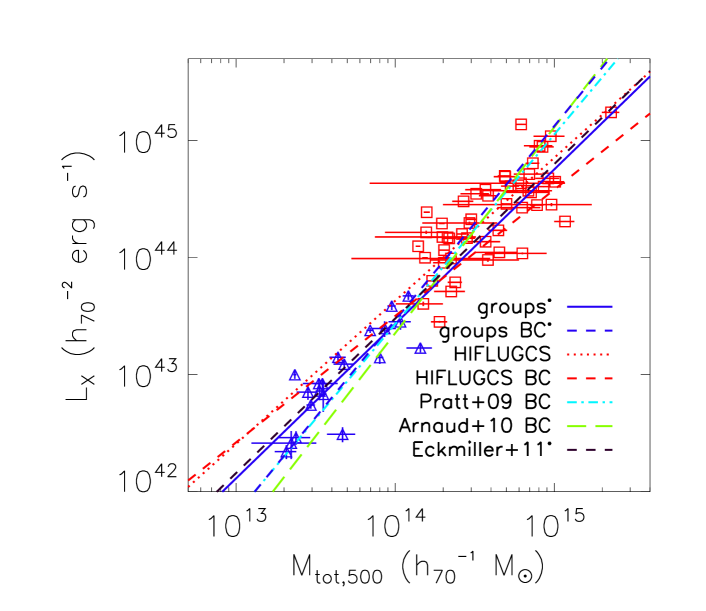
Figure 1: $L_{\text{X}}$-$M$ relation. Blue triangles are groups and red boxes are HIFLUGCS clusters with a temperature higher than 3 keV. The blue lines represent the best-fit values obtained in this work. They are compared with the best-fit results obtained with different samples. BC indicates the relation corrected for the selection bias effects. The stars indicate the works that studied galaxy groups.

5.2 Selection bias effect

5.2.1 $L_{\text{X}}$-$M$ relation

One of the most important X-ray scaling laws for cosmology with galaxy groups and clusters is the $L_{\text{X}}$-$M$ relation, because it can be used to directly convert the easiest to derive observable to the total mass.
Complete samples are required to constrain the cosmological mass function because the cluster number density must be calculated. If on one hand a flux-limited sample matches this requirement, on the other hand it suffers from the well-known Malmquist bias: brighter objects can be seen out to farther distances. From the statistical point of view, this implies that the intrinsically brighter sources will be detected more often than they ought, which distorts the sample composition. This effect has previously been taken into account for scaling relations, for example by Ikebe et al. (2002), Stanek et al. (2006), Pacaud et al. (2007), Vikhlinin et al. (2009), Pratt et al. (2009), and Mittal et al. (2011). It is important to note that proper corrections cannot be calculated for incomplete samples.
To estimate the effect of applying the sample selection ($5\times 10^{-12}\ \text{erg/s/cm${}^{2}$}\leq f_{\text{lim}}(0.1-2.4\ \text{keV})\leq 2\times 10^{-11}\ \text{erg/s/cm${}^{2}$}$ and 0.01$\leq$z$\leq$0.035) we applied the same flux and redshift thresholds to a set of simulated samples. By using the halo mass function derived by Tinker et al. (2008) with the transfer-function from Eisenstein & Hu (1998), the density fluctuation amplitude at 8 Mpc/$h$ $\sigma_{8}$=0.811 and a spectral index of the primordial power spectrum $n_{s}$=0.967 (Komatsu et al. 2011), we obtained the mass and redshift for all the simulated objects. We applied a lower mass threshold of M$>$5$\times 10^{12}$M_☉ to ensure that we selected groups and not galaxies, and an upper threshold M$<$5$\times 10^{15}$M_☉ (above this mass there are only a few clusters that are not important for this work). We then assigned a luminosity through the $L_{\text{X}}$-$M$ relation to every object and also introduced the total scatter we derived in Sect. 5.6. We note, that the scatter should only be introduced in the $L_{\text{X}}$ direction because otherwise the value of the total masses that we derived directly from the mass function would be changed as well. Since for all the BCES estimator except $Y|X$ the minimization is not purely performed in the Y (i.e., $L_{\text{X}}$) direction, they were not used for the selection bias correction.
We assigned the same error (i.e., the mean relative error derived in our analysis) to every simulated object because we did not see any particular trend in the distribution of the statistical measurements errors as function of mass or luminosity. The slope and normalization of the input $L_{\text{X}}$-$M$ relation were varied in the range [1.20:2.20] (with steps of 0.01) and [-0.15:0.05] (with steps of 0.01), respectively. For each grid point (i.e., every combination of slopes and normalizations) 300 artificial flux-limited group samples were simulated. The input slope ($a_{{\rm sim}}$) and normalization ($b_{{\rm sim}}$) that after applying the flux and redshifts cuts (to reproduce the same selection effects of our sample) yields an $L_{\text{X}}$-$M$ relation that matched the observed relation are the values corrected for the selection bias. We searched for the best combination of values by minimizing the following equation:

$$\chi^{2}_{{\rm tot}}=\frac{(\tilde{b}_{{\rm sim}}-b_{{\rm obs}})^{2}}{\Delta b_{{\rm obs}}^{2}}+\frac{(\tilde{a}_{{\rm sim}}-a_{{\rm obs}})^{2}}{\Delta a_{{\rm obs}}^{2}},$$ (10)

where $\tilde{b}_{sim}$ and $\tilde{a}_{sim}$ are the median values for the normalization and slope of the 300 output relations of each grid point. The total number of objects obtained by using the halo mass function was scaled such that the distribution of the simulated samples peaked at about 20 objects as the real sample. The scatter of the best-fit output relation after the flux and redshift cuts agrees with the observed scatter. We also verified that the luminosity and mass distribution of the simulated objects after the flux and redshift cuts matched the observed one. The correction was then also applied to the HIFLUGCS (kT$>$3 keV) and full sample (i.e., groups plus all the HIFLUGCS objects).
The $L_{\text{X}}$-$M$ relations corrected for selection bias are shown in Fig. 1 and are compared with the observed relations. The corrected relation for galaxy groups is steeper (slope of 1.66$\pm$0.22) than the observed relation ($a$=1.32$\pm$0.24). In contrast the corrected relation for massive systems was found to be slightly shallower than what is observed. Interestingly, the slope of the corrected relation remains unchanged when including all the objects in the sample (groups and HIFLUGCS). The errors of the corrected slopes were obtained from the distribution of the $\chi^{2}_{{\rm tot}}$ in the grid. For each parameter (i.e., slope and normalization) the error was derived by keeping the other interesting parameter frozen and by searching for the range of values with a $\chi^{2}_{tot}<\chi^{2}_{min}+1$.

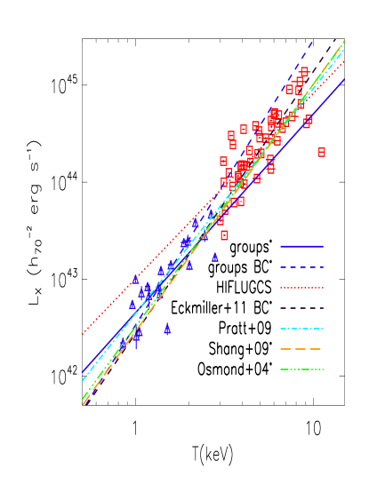
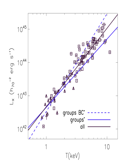
Figure 2: Left: $L_{\text{X}}-T$ relation. Blue triangles are groups, red boxes are HIFLUGCS clusters with a temperature higher than 3 keV. The stars indicate the works that studied galaxy groups. Right: Same points as in the left panel plus the HIFLUGCS clusters with a temperature lower than 3 keV. BC indicates the relation corrected for the selection bias effects.

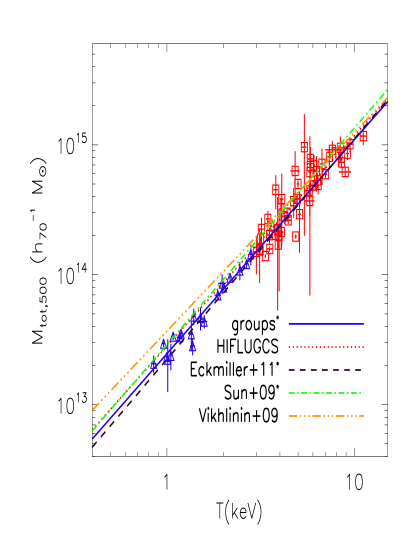
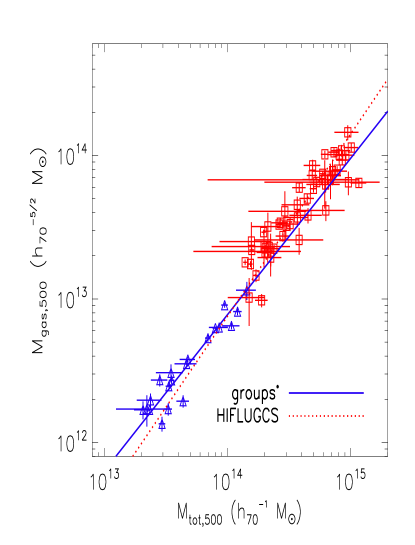
Figure 3: Left: $M$-$T$ relation. Blue triangles are groups, red boxes are HIFLUGCS clusters with a temperature higher than 3 keV. Right: same as in the left panel, but for the $M_{\text{gas}}$-$M$ relation.

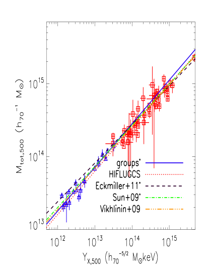
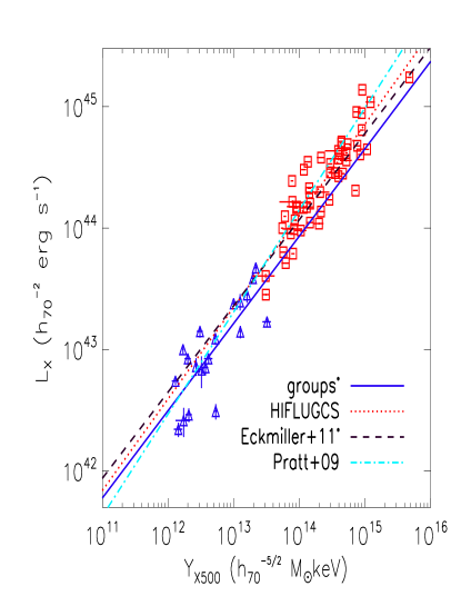
Figure 4: Left: $M$-$Y_{\text{X}}$ relation. Blue triangles are groups, red boxes are HIFLUGCS clusters. Right: same as in the left panel, but for the $L$-$Y_{\text{X}}$.

5.2.2 $L_{\text{X}}$-$T$ relation

When the “true” $L_{\text{X}}$-$M$ relation is recovered, the result can be used to derive the corrected $L_{\text{X}}$-$T$ relation. Following the procedure presented in the previous section, we assigned a luminosity to all the objects using the $L_{\text{X}}$-$M$ relation corrected for selection biases by also introducing the total scatter along the Y($L_{\text{X}}$) direction. We then assigned the temperatures through an input $L_{\text{X}}$-$T$ relation by creating a grid with a slope and normalization in the range [2.5:3.5] and [0.10:0.55]. After applying the flux and redshift cuts in the same way as for our group sample, we compared the simulated and observed $M$-$T$ relations under the assumption that this relation is unbiased. The best-fit values are the ones that minimize the $\chi^{2}_{tot}$ of Eq. 10.
In Fig. 2 (left panel) we compare the observed $L_{\text{X}}$-$T$ relation for galaxy groups with the one determined using the HIFLUGCS sample. Again, as for the $L_{\text{X}}$-$M$ relation, we do not see any steepening at the group scale. In Fig. 2 (right panel) we compare the corrected luminosity-temperature relation derived for the group sample with the observed relation. While the observed slope of our group sample, given the large errors (see Table 4), is consistent with the slope derived with massive systems, the corrected slope shows a steepening.
By fitting all the objects of our group sample and the HIFLUGCS objects, the relation becomes steeper (see right panel of Fig. 2), probably because of the different normalizations of the two samples. This effect is not significant given the uncertainties.

5.3 $M$-$T$, $M_{\text{gas}}$-$M$, and $L_{\text{X}}$-$M_{\text{gas}}$ relations

The $M$-$T$ relation is expected to follow the same behavior for galaxy groups and galaxy clusters because it is less affected by heating and cooling processes, which are thought to be responsible for the steeper relations observed in other analysis at the group scale (e.g., Eckmiller et al. 2011). Indeed, the slopes we found for the group and cluster samples are very similar (see Table 4). Even when fitting the HIFLUGCS together with the group sample we do not see any steepening. Both groups and clusters show a slope slightly steeper than the one predicted by the self-similar scenario. Kettula et al. 2013 suggested that X-ray masses are biased down due to the assumption of hydrostatic equilibrium with a larger bias for low mass systems that cause the steepening. However, a stronger bias for groups appears to be in tension with the finding of Israel et al. 2014 who find the opposite trend.
Arnaud et al. (2005) analyzed a sample of massive clusters and showed that the slope of the $M$-$T$ relation is stable at all the overdensities. We verified whether or not this is also true at the group scale by fitting the relation at $R_{2500}$ and $R_{1000}$ as well. We found that the slope is quite stable: 1.61$\pm$0.07 at $R_{2500}$, 1.71$\pm$0.13 at $R_{1000}$, and 1.65$\pm$0.11 at $R_{500}$.
In Fig. 3 (right panel) we show the fit to the $M_{\text{gas}}$-$M$ relation. Galaxy groups have a shallower slope than clusters, but the slopes agree well within the errors. The slope of the galaxy group sample also agrees well with the slope from clusters moving from $R_{2500}$ to $R_{500}$. If the gas fraction of galaxy clusters is universal. we would expect that the gas mass is linearly related to the total mass. A slope greater than one of this relation implies a trend to lower gas fraction for objects with lower temperature.
In Table 4 we also summarize the best-fit results for the $L_{\text{X}}$-$M_{\text{gas}}$ relation. Although the relation is slightly shallower at the group scale, the result still agrees within the error bars with the value obtained for the more massive systems.

5.4 $M$-$Y_{\text{X}}$ and $L_{\text{X}}$-$Y_{\text{X}}$ relations

The $Y_{\text{X}}$ parameter defined by Kravtsov et al. (2006) is considered one of the less scattered mass proxies, although this is still a matter of debate (see Stanek et al. 2010). In Fig. 4 (left panel) we show the $M$-$Y_{\text{X}}$ relation obtained for the groups and the HIFLUGCS samples. Our best fit for the slope (0.60$\pm$0.03) is aligned well with the slope of the massive systems (0.59$\pm$0.03). This means that for this relation we do not observe any hint of steepening at low masses either. The slopes are also very close to the value predicted by the self-similar scenario. Even when fitting galaxy groups and HIFLUGCS together, the best-fit is close to the self-similar prediction.
An indirect way of using the $Y_{\text{X}}$ parameter to constrain the mass is to use the $L_{\text{X}}$-$Y_{\text{X}}$ relation to reduce the scatter in the $L_{\text{X}}$-$M$ relation (Maughan 2007). The result is shown in Fig. 4 (right panel). We do not observe a steepening at low masses for this relation either (see Table 4).

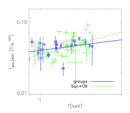
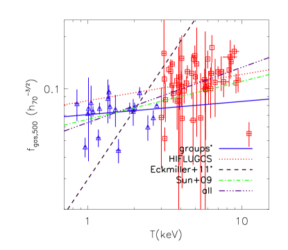
Figure 5: Left: $f_{\text{gas}}$-$T$ relation at $R_{2500}$ compared with the result by Sun et al. (2009). Right: $f_{\text{gas}}$-$T$ relation at $R_{500}$.

5.5 Gas fraction

In Fig. 5 we show the $f_{\text{gas}}$-$T$ relation at $R_{2500}$ (left panel) and $R_{500}$ (right panel). The best-fit relation is in good agreement with that obtained by Sun et al. (2009) analyzing 43 galaxy groups. The weighted mean gas fraction within $R_{2500}$ obtained for our sample is 0.049$\pm$0.001, which is slightly higher than the weighted mean of 0.047$\pm$0.001 found by Sun et al. (2009). This can also be seen from the marginally higher normalization at 1 keV found in this work compared with the result by Sun et al. (2009) in Fig. 5 (left panel). However, because the gas fraction is temperature dependent, the weighted mean gas fraction depends on the temperature distribution of the objects in the samples.
The $f_{\text{gas}}$ at $R_{2500}$ that we determined is on average 37$\%$ lower than the $f_{\text{gas}}$ at $R_{500}$. Both groups and high mass systems have a slope that agrees within the errors, although with a lower normalization for the low-mass objects. This indicates a higher gas fraction for the most massive objects. This trend of higher gas fraction for increasing masses can also be seen in the steepening of the relation when all the objects were fitted together (see Fig. 5, right panel).

5.6 Scatter

Due to their shallower potential well, galaxy groups are expected to be much more affected by non-gravitational processes than galaxy clusters. Therefore it is a common thought that galaxy groups show a larger intrinsic scatter in the X-ray scaling relations, although to our knowledge only Eckmiller et al. (2011) extensively quantified this for galaxy groups for several scaling relations and directly compared this with the scatter obtained with HIFLUGCS sample. Indeed, they found that galaxy groups in general show a larger dispersion from the best fit of the scaling relations.
In Table 5 we summarize the results for the analysis of the scatter obtained in this work. In general, the sample of galaxy groups seems to be less scattered than the sample of galaxy clusters, although the values are similar and might be consistent within the errors.
The statistical scatter in the $M$-$T$, $M_{\text{gas}}$-$M$, and $M$-$Y_{\text{X}}$ relations is lower for low-mass systems, which might be due to the better determination of the low temperatures because of the larger effective area of the current instruments at low energies and the stronger line emission. This then translates into lower mass uncertainty and a lower total scatter. Anyway, the statistical scatter for these relations dominates and the intrinsic scatter is consistent with zero.

6 Discussion

The galaxy group sample we studied together with the HIFLUGCS data have allowed us to investigate the effect of the selection bias and to study systematic differences between the scaling properties of low- and high-mass systems. We did not perform any morphological study because of the poor statistics in our sample, in particular for the unrelaxed objects. By using the central cooling time to classify the objects, we found that only three groups in our sample can be considered disturbed. In the next sections we discuss the results of our analysis in more detail.

Table 5: Scatter results using the values from the $Y|X$ fits. The scatter for the $M$-$T$, $M_{\text{gas}}$-$M$ and $M$-$Y_{\text{X}}$ relations is not listed because the intrinsic scatter is consistent with zero.

$$\centering\begin{array}[]{cccccc}\hline\cr\hline\cr\vskip 3.0pt plus 1.0pt minus 1.0pt\cr{\rm Relation}&{\rm Sample}&{\rm\sigma_{tot}(X)}&{\rm\sigma_{int}(X)}&{\rm\sigma_{tot}(Y)}&{\rm\sigma_{int}(Y)}\\ \vskip 3.0pt plus 1.0pt minus 1.0pt\cr\hline\cr&{\rm groups}&0.157&0.139&0.207&0.184\\ {\rm L_{\text{X}}-M}&{\rm HIFLUGCS\ (kT>3\ keV)}&0.210&0.185&0.265&0.234\\ &{\rm all}&0.197&0.175&0.275&0.245\\ \hline\cr&{\rm groups}&0.103&0.099&0.211&0.204\\ {\rm L_{\text{X}}-T}&{\rm HIFLUGCS\ (kT>3\ keV)}&0.119&0.118&0.228&0.227\\ &{\rm all}&0.104&0.103&0.245&0.243\\ \hline\cr&{\rm groups}&0.317&0.305&0.228&0.219\\ {\rm L_{\text{X}}-Y_{\text{X}}}&{\rm HIFLUGCS\ (kT>3\ keV)}&0.231&0.224&0.174&0.168\\ &{\rm all}&0.284&0.278&0.225&0.220\\ \hline\cr\end{array}\@add@centering$$

6.1 Selection bias

Any survey of galaxy systems provides catalogs that are somewhat biased because of the chosen survey strategy or simply because of the finite sensitivity of the instruments (see Giodini et al. 2013). A complete sample is required to be able to calculate and correct for these biases. Thanks to our simple selection, we were able to construct simulated samples, which were required to apply the corrections. The $L_{\text{X}}$-$M$ relation for the groups we analyzed, corrected for selection effects, is adequately described by a power law with a slope and normalization equal to 1.66$\pm$0.22 and -0.03$\pm$0.04. The corrected slope is steeper than the observed slope (i.e., 1.32$\pm$0.24) and has a lower normalization. This change in slope is larger than any other systematic effect we studied (e.g., cluster sample, fitting method). This result highlights the importance of correcting the observed scaling relations for selection effects. In fact, X-ray surveys such as eROSITA require proper and precise scaling relations to determine the proper cluster number density and so constrain the correct cosmological mass function.
As a result of the relatively small sample we analyzed, the uncertainty on the slope is unfortunately still quite large and a larger complete sample is required to place a stronger constraint on the necessary correction. Unlike the galaxy groups, the more massive systems (i.e., HIFLUGCS clusters with a $kT>3$ keV) return a shallower corrected slope. One possible explanation is that the true $L_{\text{X}}$-$M$ relation is gradually steepening when moving toward the low-mass objects. In this case, higher temperature cuts would result in shallower relations. To verify this, we tested by applying different cuts whether the true relation that we obtained after the bias correction is temperature dependent. Indeed, the corrected $L_{\text{X}}$-$M$ relation steepens when lowering the temperature cut. For comparison with the value quoted in Table 4, the corrected slope is 1.25$\pm$0.22 and 1.13$\pm$0.21 when applying a cut to the HIFLUGCS sample at 1 and 2 keV. This result would suggest a break in the $L_{\text{X}}$-$M$ relation after correcting for the selection bias effects. This would be very important for future X-ray surveys because it would imply that a simple power law cannot be used to convert the measured luminosities (or temperatures) into masses. For a quick reference we provide here the corrected $L_{\text{X}}$-$M$ relation:

$$L_{\text{X}}=\bigg{\{}\begin{array}[]{rl}1.70\cdot 10^{20}M^{1.66};&M\lesssim 10^{14}M_{\odot}\\ 2.43\cdot 10^{28}M^{1.08};&M\gtrsim 10^{14}M_{\odot}.\\ \end{array}$$ (11)

Moreover, we note that our corrected slope for the massive systems is much shallower than the slope obtained for example, by Pratt et al. (2009) and Arnaud et al. (2010).
The uncorrected observed $L_{\text{X}}$-$T$ relation behaves quite similarly to that of the uncorrected $L_{\text{X}}$-$M$. The observed slope of our group sample is consistent within the errors with that of the clusters and in general with the results from other papers investigating galaxy groups (e.g., Osmond & Ponman 2004; Shang & Scharf 2009; Eckmiller et al. 2011). Because the emissivity at low temperatures scales with $T^{-0.6}$ (McKee & Cowie 1977), the relation predicted by the self-similar scenario for galaxy groups is $L_{\text{X}}\propto T^{1.1}$, which is flatter than the observed relation. Thanks to the corrected $L_{\text{X}}$-$M$ relation, we were also able to correct the $L_{\text{X}}$-$T$ relation for the selection bias effects. Similarly to the $L_{\text{X}}$-$M$ relation, the $L_{\text{X}}$-$T$ is steeper that the observed relation when the selection bias effects are taken into account with a steepening in the low-mass regime. Our result agrees qualitatively quite well with the findings of Eckmiller et al. (2011) (but note that their group sample is incomplete) and Mittal et al. (2011), who corrected the $L_{\text{X}}$-$T$ relation for the HIFLUGCS clusters. Since they used the bolometric luminosities, we cannot directly compare their results with our relations.

6.1.1 Group luminosities and completeness of the sample

The corrected relations we obtained are based on the assumption that we deteced all the objects above a certain flux. Because of the shallow observation of the RASS data some of the faint objects might be missing from the REFLEX and NORAS input catalogs, or that their estimated flux fell below our limit. To check this, we estimated the luminosities using the SB and k$T$ profiles derived in this work and compared them with the values in the input catalogs. The new X-ray luminosities were estimated by integrating the X-ray surface brightness up to the $R_{500}$. Basically, for all the annuli used to derive the temperature profiles we estimated the total count rate from the SB profile and converted this to the X-ray luminosity using the best-fit temperature and abundance values obtained during the spectral analysis. Since our data only cover a fraction of $R_{500}$, the temperatures to convert the count rate to the luminosity beyond the detection radius were set to an average value given by the extrapolated temperature profiles with an abundance frozen to 0.3 solar. The results are summarized in the Table 2. While for most of the objects the luminosity estimated using the XMM-Newton data agree quite well within the errors with the ROSAT luminosities, for some very low mass objects our estimated luminosity is much higher. If on one hand the large extrapolation of the profiles makes these measurements quite uncertain, it might be that ROSAT was only able to detect a small fraction of the $R_{500}$ because of their faint emission in the outer region . As a consequence, is also possible that some of the objects with the lowest flux are missing and that the input catalogs are more incomplete than previously thought.

6.2 Mass proxies

Among all the mass proxies, the $Y_{\text{X}}$ parameter seems the most promising one to be used with the next X-ray surveys. In contrast to $M_{\text{gas}}$, $L_{\text{X}}$, and $T$ the agreement between the slope and normalization of different works (e.g., Arnaud et al. 2007; Maughan 2007; Vikhlinin et al. 2009; Sun et al. 2009) is very good and is very close to the self-similar scenario independently of the fitting method. This is probably because the $Y_{\text{X}}$ parameter is related to the total thermal energy of the ICM, which is mainly associated with the gravitational processes and so is less sensitive to any feedback. It is also useful to note that despite the different fraction of unrelaxed systems in the samples, the slope remains stable, which confirms that indeed the $M$-$Y_{\text{X}}$ relation is quite insensitive to the dynamical state of the objects. A direct implication is that if the eROSITA data will allow us to measure the temperature and SB profiles for many galaxy groups and clusters we will be able to estimate the total mass from the $M$-$Y_{\text{X}}$ relation. While Borm et al. (2014) found that at least an overall temperature can be obtained with good accuracy (errors lower than 10$\%$) for $\sim 2,000$ objects, determining the surface brightness profiles might be more complicated because of the eROSITA PSF.
Indeed, given the expectation for the temperature determination with eROSITA, it would be much more straightforward to use the $M$-$T$ relation to estimate the mass. Unfortunately, simulations (e.g., Evrard et al. 1996, Nagai et al. 2007) show that masses are underestimated by up to 20$\%$ for merging systems because the assumptions of hydrostatic equilibrium and spherical symmetry are invalid. Thus, a different fraction of merging systems in the analyzed sample would result in a different slope and normalization. Although our slopes agree well with the slopes in literature, in particular the slopes obtained using samples of galaxy groups, the normalization of the $M$-$T$ relation is $\sim$15$\%$ lower than the normalization obtained by Sun et al. (2009) and $\sim$5$\%$ higher than that obtained by Eckmiller et al. (2011).
The $M_{\text{gas}}$-$M$ relation has been suggested as the lowest scattered mass proxy. Although the slopes for galaxy groups and clusters are quite similar, there is some indication of steepening for high-mass systems. This then translates into an even higher gas mass and so higher gas fractions for a given total mass, than is actually observed.

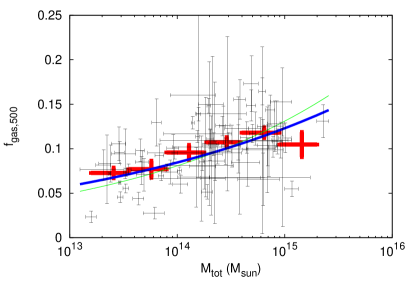
Figure 6: Gas fraction as a function of the total mass. The black points represent the single objects (groups and HIFLUGCS), the red points are the mean values. The error bars are the standard errors. The solid blue line represents the best fit to the unbinned data. The parameters are listed in Table 4. The green line represents the best fit obtained by Pratt et al. (2009).

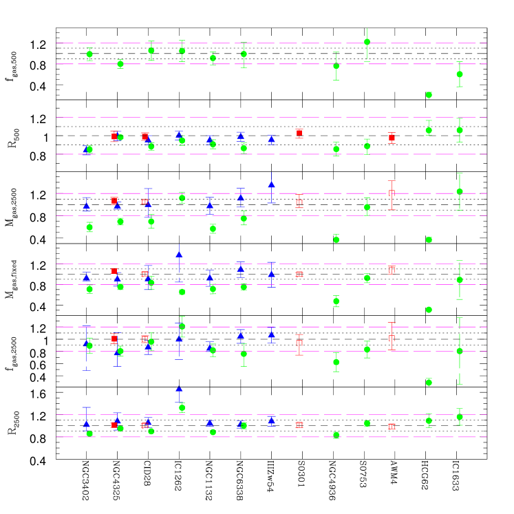
Figure 7: Comparison between the ratio of the results obtained in this work with the results reported by Gastaldello et al. 2007 ($R_{2500}$: filled red squares; $R_{1250}$: empty red squares), Sun et al. 2009 (blue triangles), and Eckmiller et al. (2011) (green circles). From bottom to top we compare the ratio of $R_{\text{2500}}$; $f_{\text{gas,2500}}$; $M_{\text{gas}}$ at the fixed $R_{\text{2500}}$ by Gastaldello et al. (2007), Sun et al. (2009), and Eckmiller et al. (2011) with this work; $f_{\text{gas,2500}}$; $R_{\text{500}}$; and $f_{\text{gas,500}}$, respectively.

6.3 Gas fraction

Several independent analyses have found that the fraction of gas in galaxy clusters decreases when moving toward lower mass systems (e.g., Sanderson et al. 2003; Vikhlinin et al. 2006; Gastaldello et al. 2007; Pratt et al. 2009). Pratt et al. (2009) showed the tendency of the gas mass fraction versus total mass by using data from different works. While the massive system domain was well represented, the sample they built had only a few low-mass systems (e.g., only five objects with $M<5\times 10^{13}M_{\odot}$). Our master sample has almost four times more objects at low masses and is more than two times larger in total. In Fig. 6 we show the results for our sample. The behavior is similar to the one found by Pratt et al. (2009) with an increase of the gas fraction within $R_{500}$ with mass and a hint of flattening at the lowest ($<$$10^{14}M_{\odot}$) and highest masses ($>$$10^{15}M_{\odot}$).
In the review by Sun (2012) about galaxy groups, the author compared the gas fractions obtained in different papers (i.e., Vikhlinin et al. 2006; Gastaldello et al. 2007; Sun et al. 2009; Eckmiller et al. 2011) and found that while the first three agree relatively well, the gas fraction estimated by Eckmiller et al. (2011) has a mean nonsystematic deviation of $\sim 20\%$ for most groups and a much larger offset toward the low side for four groups (which are not in our sample). Sun (2012) suggested that the difference may come from the limited coverage of the group emission by the Chandra data, the background treatment performed by Eckmiller et al. (2011), and the simpler models adopted by Eckmiller et al. (2011) to describe the temperature and surface brightness profiles. Apart from the parametrization of the temperature profiles, our approach is quite similar to the approach presented by Eckmiller et al. (2011), therefore we update the plot by Sun (2012) with our results (see Fig. 7) to check whether they are consistent with previous works. Our estimated radii agrees generally well with the other works. Nevertheless, by comparing the temperatures of the objects in common between the samples we found that our global temperature is 13$\%$ higher than the temperatures obtained by Sun et al. (2009) (in agreement with the different AtomDB results, see Appendix A), while the temperatures by Eckmiller et al. (2011) agree well within $5\%$ (except for three objects) with the temperatures in this work. Thus, although our global temperatures are in general higher than the ones derived by Sun et al. (2009), the estimated total masses are slightly lower. A possible explanation is that our density profiles are flatter in the outer region, causing slighter lower total masses.
At $R_{2500}$ the gas fraction of all the objects in common with Sun et al. (2009), except for IC1262, agree to at maximum $20\%$ with a mean nonsystematic deviation of $\sim$10$\%$. Four out of ten objects in common with Eckmiller et al. (2011) have a gas fraction systematically lower than our finding with a deviation larger than 25$\%$, and the mean deviation for the others 6 is $\sim$15$\%$ (only for IC1262 our gas fraction is lower than the gas fraction found by Eckmiller et al. 2011). We have only four groups in common with Gastaldello et al. (2007), and for three of them they provided only the gas fraction at an overdensity of 1250. Therefore we computed the gas fraction for these three groups at the same overdensity and obtained a very good agreement. For a more direct comparison we then recomputed our gas masses at the radii ($R_{\Delta}$) derived by Gastaldello et al. (2007), Sun et al. (2009), and Eckmiller et al. (2011). The result is shown in Fig. 7 (third panel). The gas masses from Sun et al. (2009), Gastaldello et al. (2007), and this work agree to $\sim$10$\%$, while the gas masses from Eckmiller et al. (2011) are very low (seven out of ten objects have a gas mass lower by 25-75$\%$ than our finding). To investigate the cause of the difference with Eckmiller et al. (2011), we calculated the gas masses at the $R_{2500}$ quoted in their paper using the best fit values of their surface brightness and central electron densities (private communication) with our code. For most of the objects the gas masses we obtained are different from the masses calculated by Eckmiller et al. (2011) but agree with the ones obtained in this work. There are still a few objects (HCG62, IC1633, NGC3402, and S0753) for which the differences are still significantly high. Thus, apart from a possible inaccuracy in the code, there might be other effects (e.g., the effects suggested by Sun 2012) that cause the observed discrepancies between our results and those of Eckmiller et al. (2011). However, the result shows that the strong difference for the $f_{\text{gas}}$ values found by Eckmiller et al. (2011) does not mainly arise from a simpler analysis, as our agreement with Sun et al. (2009) and Gastaldello et al. (2007) suggests, but probably by an incorrect calculation of the gas masses, which may also affect their scatter estimates (see Sect. 5.6).
We then investigated which kind of groups contributed more to the scatter of the scaling relations. Interestingly, we found that the groups with higher gas fraction within $R_{2500}$ deviate more from the best fit of the scaling relations. For example, the mean deviation from the best fit of the L-T relation for the ten objects with lower gas fraction is 0.31, while for the objects with higher gas fraction within $R_{2500}$ is 0.82 (0.58 if we do not consider IC1633 which deviates more).

6.4 Scatter

Low-mass systems show a similar and sometimes even smaller intrinsic scatter than their massive counterparts. If, on one hand, this result contradicts the common thought of groups having a larger scatter, on the other hand it is expected from the result of the previous section. In fact, since the groups contributing more to the scatter are the ones with the higher gas fraction, it is expected that galaxy clusters that generally have an even higher gas fraction show a larger dispersion in the scaling relations. Mittal et al. (2011) analyzed the HIFLUGCS sample and found that objects with a CRS have a smaller scatter than objects without. Since the fraction of objects in the group sample with a CRS is larger that the fraction in the massive systems, our result agree with the finding of Mittal et al. (2011).
However, the properties of the massive clusters were obtained using an isothermal model and a single $beta$-model (Reiprich & Böhringer 2002) and not a temperature profile like for the groups in this work. Together with the larger fraction of disturbed systems in the HIFLUGCS sample and the fact that in this analysis a strong extrapolation is required to estimate the group properties, this might partially explain the lower scatter observed at the group scale.

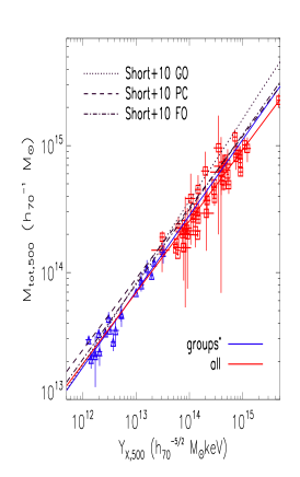
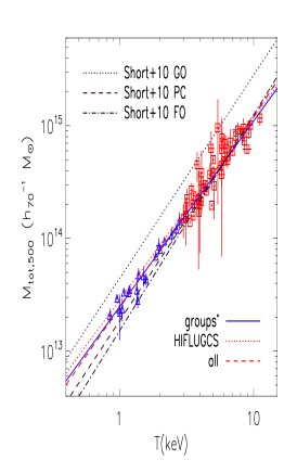
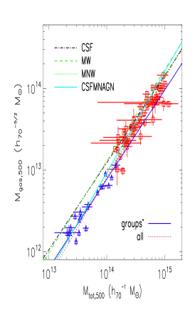
Figure 8: Left: The best-fit $M$-$Y_{\text{X}}$ relations determined in this work are compared with the results from Short et al. (2010). Center: As in the left panel, but for the $M$-$T$ relation. Right: The best-fit $M_{\text{tot}}$-$M_{\text{gas}}$ relations determined in this work are compared with the results from Fabjan et al. (2010).

6.5 Comparison with simulations

A direct comparison between the observed scaling relations and the results from hydrodynamical simulations can give us information about the processes that play a role in the ICM at different masses. We investigate the mass-proxies relations by comparing the data with the simulation of Short et al. (2010) for the $M$-$T$ and $M$-$Y_{\text{X}}$ relations, and Fabjan et al. (2011) for the $M_{\text{gas}}$-$M$. The results for the $M$-$T$ and $M$-$Y_{\text{X}}$ relations by Fabjan et al. (2011) were not used because of the known difference between the mass-weighted temperature used in their paper and the spectroscopic temperature (Mazzotta et al. 2004).
In the $M$-$Y_{\text{X}}$ relation, the gravitational heating alone (black dotted line in the left panel of Fig. 8) is not enough to match the observational data, and additional processes have to be included. The slope obtained by Short et al. (2010) when including only the gravitational processes in the simulations is steeper than the slope predicted by the self-similar scenario, which was quite well reproduced when the non-gravitational heating was included in the simulations. Thus, on one hand the observed relation seems weakly affected by the non gravitational processes (confirmed also by the fact that the relation shows the same slope at all the masses), on the other hand, simulations need to include feedback to match the observed slope. Although our slope agrees well with the prediction from Short et al. (2010) when the energy input from supernovae and AGNs (FO run) were included, the normalization is $\sim$14$\%$ lower than the prediction from their simulation.
The observational results for the $M$-$T$ relation compared with the predictions by Short et al. (2010) are shown in the center panel of Fig. 8. Although at high masses there is a good agreement (difference $<$10$\%$ at 10 keV) in the low-mass regime, there is a strong difference ($\sim 25\%$ at 1 keV) between our observational results and the simulations. On the other hand, they neglect cooling processes so that systems with a cool-core are not formed, whiche prevents a comparison with our group sample that contains a large fraction of such systems. Thus, the mismatch between observation and simulations requires further investigations.
The $M_{\text{gas}}$-$M$ relation (right panel of Fig. 8) of our group sample agrees to better than 10$\%$ at 5$\times$10${}^{13}M_{\rm sun}$ with the finding of Fabjan et al. (2011) when they include AGNs feedback. In contrast, when only galactic winds are included in the simulations, there is a strong disagreement with the observations (e.g., $>$50$\%$ at 5$\times$10${}^{13}M_{\rm sun}$). Together with the lower gas fraction in galaxy groups, these results suggest that indeed AGN activity is at work and that this is probably responsible for transporting the gas away from the galaxy group center.
In general, simulations including feedback processes are able to reproduce the observed slope and normalization better than the simulations including only gravitational effects. On the other hand, their effect does not strongly affects the slope (i.e., we do not observe any break in the scaling relations as also found for the L-T relation by Gaspari et al. 2014 when the self-regulated kinetic feedback model is adopted in the simulations) in the low-mass regime, although it is possible that their contribution decreases gradually with the mass of the systems and is then hidden by the scatter.

7 Conclusions

The complete sample of galaxy groups studied in this paper allowed us to correct the $L_{\text{X}}$-$M$ and $L_{\text{X}}$-$T$ relation for selection bias effects. While selection biases have been taken into account in several papers analyzing complete samples of galaxy clusters (including some groups), this is the first time that this was done for a complete sample of local X-ray selected groups. We summarize our results as follows:

1. The slope (1.66$\pm$0.22) of the $L_{\text{X}}$-$M$ relation corrected for the selection bias effects, derived at the group scale, is steeper than the corrected slope (1.08$\pm$0.21) obtained with massive systems. If confirmed with larger samples, this would imply that for future X-ray surveys such as eROSITA a relation with more freedom than a single power law to convert the luminosities into the total masses is required to constrain the cosmological parameters.

2. For the other mass proxies we found that the $M$-$Y_{\text{X}}$ relation seems less sensitive to the dynamical state of the objects and consequently, to the sample properties.

3. In general, we did not observe any steepening of the observed uncorrected scaling relations in the low-mass regime.

4. Groups have an intrinsic scatter similar or even smaller than the scatter derived for galaxy clusters.

5. The observed scaling relations for galaxy groups agree well with the simulations including AGNs, although it depends strongly on the physical processes included in the simulations. This indicates that non-gravitational processes play an important role in the evolution of galaxy groups.

6. The gas mass fraction in galaxy groups is almost a factor of two lower than the gas fraction in galaxy clusters.

7. The new improved AtomDB version yields a gas fraction up to 20$\%$ lower than an older version.

Appendix A AtomDB

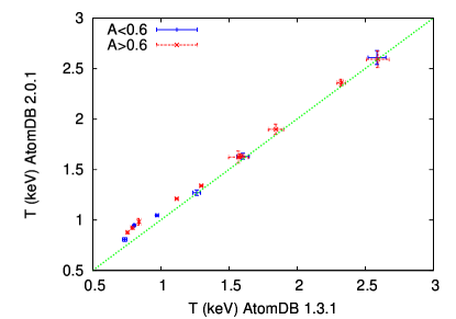
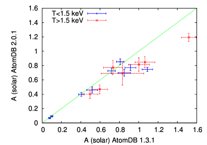
Figure 9: Left: comparison between the temperatures determined using the old version 1.3.1 and the new version 2.0.1 of AtomDB. Different colors represent groups with an abundance higher (red) and lower (blue) than 0.6 solar. Here, we plotted only the innermost temperature bin, and excluded the groups for which we determined only a global temperature: IC1262, NGC6338, RXCJ1840. Right: the same as in the left panel, but comparing the abundances instead of the temperatures. Different colors represent groups with a temperature higher (red) and lower (blue) than 1.5 keV.

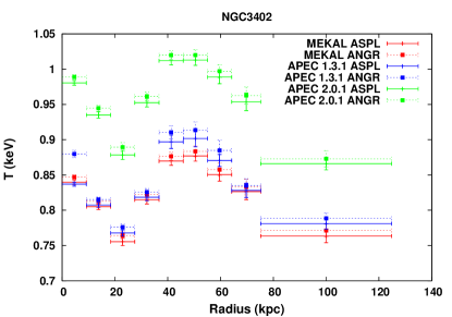
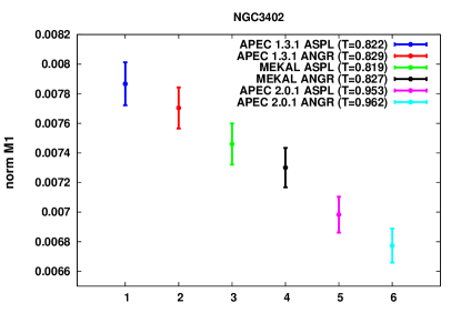
Figure 10: Left: temperature profile of NGC3402 derived by fitting the spectra with different plasma models and abundance tables. Right: normalization values obtained by fitting a spectrum with different plasma models and abundance tables.

Version 2.0 of AtomDB is available since 2011. With respect to the older version 1.3, it includes significant improvements on the iron L-shell data. As we show below, this change strongly affects the temperature and abundance determination for low-mass systems. We used the temperature and the APEC normalization from the spectral fits to determine the gas and total masses. Thus, the use of different AtomDB versions has to be taken into account when comparing our results with the ones in literature. Here, we analyze the main effects.

A.1 Temperature and total mass

To show how the temperature and abundance determination change, we fitted the innermost bin of the galaxy groups in our sample using the two AtomDB versions. The results are shown in Fig. 9. While at temperatures higher than 1.5 keV the temperature difference is quite small, at very low temperatures (i.e., $kT$$<$1 keV) the temperatures obtained using the version 2.0 are up to 18$\%$ higher than the ones obtained using version 1.3. At the same time, the obtained abundance is 20-30$\%$ lower with a trend of a larger deviation for higher temperatures. More in detail, we note that when the group abundance is relatively low ($A$$<$0.6$A$_☉), the temperature deviation arises only for $kT$$<$ 1 keV. In contrast, when the abundance is relatively high ($A$$>$0.6$A$_☉), small differences can be observed already at a temperature of $\sim$2 keV.
To investigate how much this influences the total mass estimate we used NGC3402 as a test case because of its low temperature and good quality of data. Since many authors use a MEKAL model instead of the APEC model, we also included this thermal plasma model in our analysis. We determined the temperature profile for the different models and for different abundance tables (i.e., from Anders & Grevesse 1989 and Asplund et al. 2009). As shown in Fig. 10 (left panel), while the profile from MEKAL and the old AtomDB version agree quite well, the new AtomDB has a higher temperature at all radii. This translates into a total mass higher by $\sim$10$\%$. Although the effect is weak, a higher temperature is also obtained when the old abundance table from Anders & Grevesse (1989) instead of the most recent table from Asplund et al. (2009) is used.

A.2 Gas density and gas mass

In Fig. 7 we compared the gas mass at a given radius for different works and found that the difference for most of the objects is of $\sim$10$\%$. Since we used the APEC normalization to estimate the central electron densities to better understand whether the new AtomDB can explain part of the difference, we compared the normalization of the spectrum extracted from an annulus of $\sim$7 arcmin (to maximize the S/N) and fitted with the different models. As shown in the right panel of Fig. 10 (for display purposes we only show the MOS1 normalization, but the trend is similar for MOS2 and pn, although with different values), the normalization with the new AtomDB is $\sim$10$\%$ lower than the older one with the MEKAL one lying in between. Depending on the combination of abundance tables and plasma models used in a particular paper, the difference can be up to $\sim$15-20$\%$. Since the central electron density scales with the square root of the normalization from XSPEC, using the new AtomDB can give a lower central density (and so a lower integrated gas mass) of up to 7-10$\%$. The difference in gas mass for NGC3402 is $\sim$6$\%$ at $R_{2500}$ and $\sim$10$\%$ at $R_{500}$, so the use of different AtomDB versions alone can explain the different gas mass shown in Fig. 7.

A.3 Gas fraction

The use of the new AtomDB version results in a total mass higher by 10$\%$ than the mass derived using an older version. At the same time, the gas mass will be up to $10\%$ lower than the value obtained using the old AtomDB versions. Given these results, the gas fraction for the less massive galaxy groups obtained with the most recent version of the AtomDB can be up to 20$\%$ lower than the mass derived with the old AtomDB version. Of course, this is an upper limit because we used NGC3402 for the calculation, one of the coolest groups in our sample, which implies a larger difference between the different AtomDB versions, and not all the low temperature objects show such a large difference. Furthermore, in general, the temperature profiles obtained with the new AtomDB version cannot be simply scaled up because, as we showed, the difference in temperature depends both on the real temperature and on the associated metallicity. For example, in the outer regions where the temperature is lower, the metallicity is lower as well, which mitigates the real difference in the temperature estimation (see, e.g., 9). This result highlights the importance of taking this problem into account for comparisons between different papers.

Appendix B A few details on some galaxy groups

A194

At first glance, A194 can be confused with a merging system because it shows three X-ray peaks: the main one in the NE, a second one in the SW, and a third in the center. Mahdavi et al. (2005) argued that the SW source is a background cluster of galaxies at $z$=0.15. Sakelliou et al. (2008) confirmed that although it might be possible that the SW source is a background cluster, it is not possible with the XMM-Newton data to exclude that the source is at the same redshift as A194. We used an extraction area with a radius of 1 arcmin centered on the source and found that it is better fitted by a thermal plasma at redshift 0.15 than by a model with a redshift fixed at 0.018, in agreement with the finding of Mahdavi et al. (2005). In particular, we obtained a temperature of $1.82^{+0.10}_{-0.13}$ and metallicity of $0.36^{+0.05}_{-0.05}$ with $\chi^{2}/dof=137/114$ when $z$=0.15 and a temperature of $1.28^{+0.04}_{-0.04}$ and metallicity $0.10^{+0.02}_{-0.02}$ with $\chi^{2}/dof=173/114$ if $z$=0.018. Thus, since the peak is probably the BCG of a background cluster, we decided to exclude a region corresponding to $R_{500}$ from the analysis of A194 to minimize the effect that it would have on the derived properties. By using the $M$-$T$ relation derived only using the other objects in the sample, we then estimated for A194 a mass of M$\sim$6$\times 10^{13}$ and R₅₀₀$\approx$500 kpc which corresponds to about 3.5 arcmin at the A194 redshift. To be on the safe side, we excluded 4 arcmin around the SW peak. The flux in the 0.1-2.4 keV band from this 4 arcmin region is $\sim$10^-12 erg/s/cm², so even excluding this region, the net flux of A194 is $\sim$8.7$\times$10^-12 erg/s/cm², well above the flux limit threshold.
By extracting a spectrum from a region with a radius of 15^′′ around the NW source, we found that it is consistent with that of an AGN type 2 (an intrinsic absorption component was needed to fit the spectrum). The redshift of the source is 0.0182 consistent with the redshift of the cluster and a luminosity of 3$\times 10^{41}$ erg/s, suggesting that it is accreting inefficiently. The estimated flux is 1.3$\times 10^{-13}$ ergs/s/cm².
Both regions were excluded from the analysis of the group properties.

A3390

A3390 shows two X-ray peaks that are centered on two bright galaxies at the cluster redshift. We extracted a spectrum from a region of 4^′ around the two X-ray peaks to estimate the redshift of the two clumps with the X-ray data alone. We did not find any evidence that the two clumps have a different redshift. We estimated the temperature and surface brightness profiles of each component independently by excluding a region of 10 arcmin around the second subcluster.

IC1633

IC1633 appears as a relaxed group with no usual signs of a merger, such as a radio halo or a mismatch between the X-ray peak and the cD galaxy. Instead, from the exposure-corrected, background- and point-source-subtracted image we note that there is a strong elongation to the north of the emission peak (i.e., higher surface brightness). This feature together with the separation of more than 30 kpc between the EP and EWC suggests we are probably observing an unrelaxed system.

A3574E

A3574 has two components separated by $\sim$0.6 Mpc that are accepted as independent clumps (Böhringer et al. 2004). The main one is the eastern clump (A3574E), whose central galaxy is a Seyfert galaxy: IC 4329A. This galaxy carries 75$\%$ of the total flux of the clump (Böhringer et al. 2004), but the net flux of $\sim$7.3$\times$10^-12 ergs/s/cm² is still above the flux threshold of this paper.

WBL154

This system is clearly in the process of merging, with a bright subclump just to the south of the main X-ray peak.The subclump corresponds to a small group of galaxies apparently falling into the gravitational potential of the main group.

NGC4936

NGC4936 is the lowest redshift group analyzed in this sample. Its surface brightness profile has an unusual outer $\beta$ value of 0.32$\pm$0.01. The X-ray image shows that the X-ray peak, which is centered on the cD galaxy, is surrounded by a very faint extended emission.

NGC3402

Despite its overall regular and spherical X-ray emission, this galaxy group shows an anomalous temperature distribution with a central temperature peak surrounded by a relatively cool shell. This remarkable feature has also been observed by different authors (e.g., Vikhlinin et al. 2006; O’Sullivan et al. 2007; Sun et al. 2009 Eckmiller et al. 2011) and different instruments (e.g., XMM-Newton and Chandra). Combining XMM-Newton, Chandra, and VLA observations O’Sullivan et al. (2007) concluded that the most likely explanation for this feature is the interplay between the cool-core region and a previous period of AGN activity.

Appendix C Surface brightness profiles

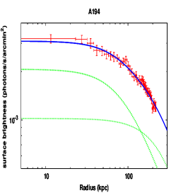
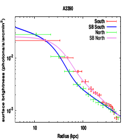
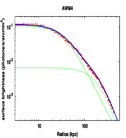
Figure 11: Surface brightness profiles for A194, A3390, and AWM4.

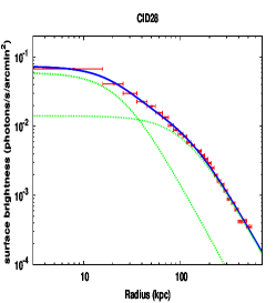
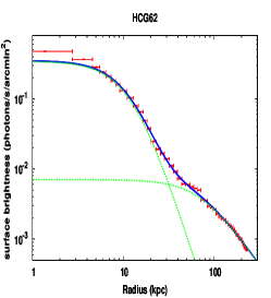
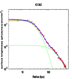
Figure 12: Surface brightness profiles for CID28, HCG62, and IC1262.

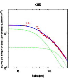
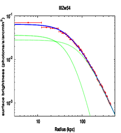
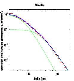
Figure 13: Surface brightness profiles for IC1633, IIIZw054, and NGC3402.

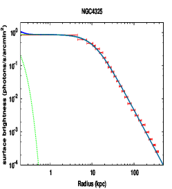
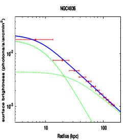
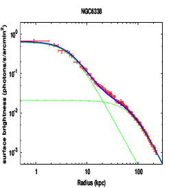
Figure 14: Surface brightness profiles for NGC4325, NGC4936, and NGC6338.

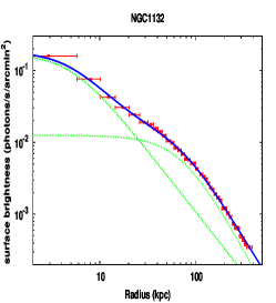
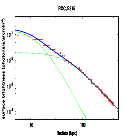
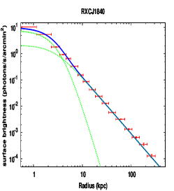
Figure 15: Surface brightness profiles for NGC1132, RXCJ2315.7-0222, and RXCJ1840.6-7709.

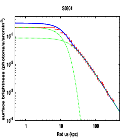
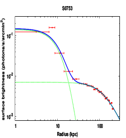
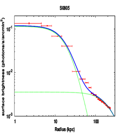
Figure 16: Surface brightness profiles for S0301, S0753, and S0805.

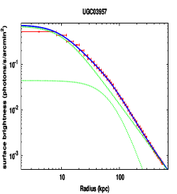
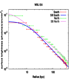
Figure 17: Surface brightness profiles for UGC03957 and WBL154.

Table 6: Fit parameters with a double $\beta$ model.

$$\centering\begin{array}[]{ccccccc}\hline\cr\hline\cr\vskip 3.0pt plus 1.0pt minus 1.0pt\cr{\rm Name}&{\rm S_{01}}&{\rm S_{02}}&{\rm\beta_{1}}&{\rm\beta_{2}}&{\rm r_{c,1}}&{\rm r_{c,2}}\\ &10^{-2}{\rm cts/s/armin^{2}}&10^{-2}{\rm cts/s/armin^{2}}&&&{\rm kpc}&{\rm kpc}\\ \hline\cr{\rm NGC4936}&1.9\pm 0.1&0.5\pm 0.1&0.494\pm 0.051&0.320\pm 0.013&11\pm 1&28\pm 2\\ {\rm S0753}&195.0\pm 34.0&0.7\pm 0.0&1.948\pm 0.342&0.583\pm 0.085&21\pm 3&140\pm 24\\ {\rm HCG62}&34.6\pm 2.6&0.7\pm 0.2&0.861\pm 0.207&0.484\pm 0.051&13\pm 3&74\pm 20\\ {\rm S0805}&91.5\pm 7.4&0.4\pm 0.0&0.915\pm 0.074&0.658\pm 0.276&15\pm 2&247\pm 88\\ {\rm NGC3402}&100.2\pm 3.2&9.7\pm 1.6&0.720\pm 0.007&0.607\pm 0.020&7\pm 1&24\pm 6\\ {\rm A194}&0.2\pm 0.0&0.1\pm 0.0&0.405\pm 0.097&0.737\pm 0.103&93\pm 23&422\pm 81\\ {\rm RXCJ1840.6-7709}&995.0\pm 47.5&18.3\pm 10.0&0.813\pm 0.071&0.518\pm 0.009&3\pm 1&8\pm 6\\ {\rm S0301}&8.0\pm 2.0&22.5\pm 6.4&0.490\pm 0.005&2.544\pm 1.565&23\pm 4&30\pm 25\\ {\rm NGC1132}&16.2\pm 0.8&1.2\pm 0.1&0.475\pm 0.007&0.612\pm 0.020&6\pm 1&84\pm 6\\ {\rm IC1633}&1.6\pm 0.1&0.3\pm 0.1&0.390\pm 0.042&0.710\pm 0.020&42\pm 5&327\pm 29\\ {\rm NGC4325}&87.7\pm 14.2&87.4\pm 1.1&6.194\pm 1.177&0.566\pm 0.003&1\pm 1&11\pm 1\\ {\rm RXCJ2315.7-0222}&8.8\pm 0.3&2.0\pm 0.0&0.959\pm 0.073&0.526\pm 0.063&23\pm 3&47\pm 8\\ {\rm NGC6338}&65.0\pm 4.8&2.9\pm 1.0&0.640\pm 0.154&0.573\pm 0.061&6\pm 2&59\pm 18\\ {\rm IIIZw054}&3.6\pm 0.6&2.8\pm 1.1&0.907\pm 0.261&0.540\pm 0.010&63\pm 24&96\pm 22\\ {\rm IC1262}&16.8\pm 1.2&1.1\pm 0.2&0.891\pm 0.120&0.600\pm 0.020&50\pm 6&221\pm 21\\ {\rm AWM4}&10.9\pm 3.0&0.7\pm 0.1&0.600\pm 0.020&0.990\pm 0.090&36\pm 5&247\pm 33\\ {\rm CID28}&5.9\pm 2.0&1.4\pm 0.1&0.590\pm 0.020&0.580\pm 0.010&24\pm 2&113\pm 4\\ {\rm UGC03957}&67.7\pm 3.3&4.4\pm 0.4&0.457\pm 0.007&0.776\pm 0.025&10\pm 2&78\pm 6\\ \hline\cr\end{array}\@add@centering$$

Appendix D Temperature profiles

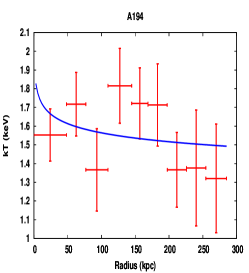
Figure 18: Temperature profiles for A194, A3390, and AWM4.

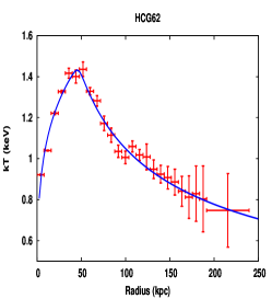
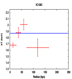
Figure 19: Temperature profiles for CID28, HCG62 and IC1262.

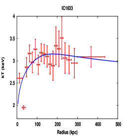
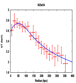
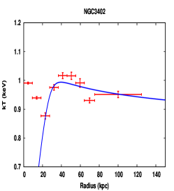
Figure 20: Temperature profiles for IC1633, IIIZw54, and NGC3402.

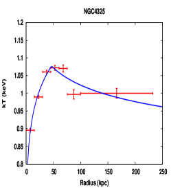
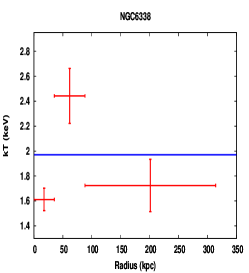
Figure 21: Temperature profiles for NGC4325, NGC4936, and NGC6338.

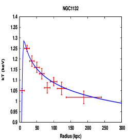
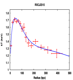
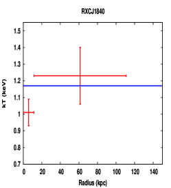
Figure 22: Temperature profiles for NGC1132, RXCJ2315.7-0222, and RXCJ1840.6-7709.

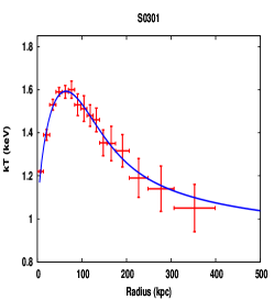
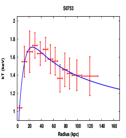
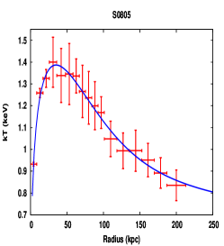
Figure 23: Temperature profiles for S0301, S0753, and S0805.

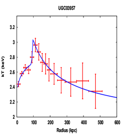
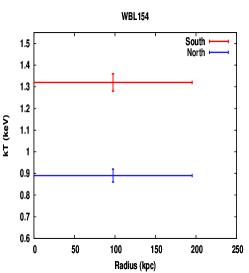
Figure 24: Temperature profiles for UGC03957 and WBL154.