COSMOLOGICAL PARAMETERS FROM SUPERNOVAE ASSOCIATED WITH GAMMA-RAY BURSTS

Abstract

We report estimates of the cosmological parameters $\Omega_{m}$ and $\Omega_{\Lambda}$ obtained using supernovae (SNe) associated with gamma-ray bursts (GRBs) at redshifts up to 0.606. Eight high-fidelity GRB-SNe with well-sampled light curves across the peak are used. We correct their peak magnitudes for a luminosity-decline rate relation to turn them into accurate standard candles with dispersion $\sigma=0.18$ mag. We also estimate the peculiar velocity of the low-redshift host galaxy of SN 1998bw, using constrained cosmological simulations. In a flat universe, the resulting Hubble diagram leads to best-fit cosmological parameters of $(\Omega_{m},\Omega_{\Lambda})=(0.58^{+0.22}_{-0.25},0.42^{+0.25}_{-0.22})$. This exploratory study suggests that GRB-SNe can potentially be used as standardizable candles to high redshifts to measure distances in the universe and constrain cosmological parameters.

1 INTRODUCTION

The accelerating expansion of the universe was detected with the help of Type Ia supernovae (SNe Ia) (Perlmutter et al. 1997; Riess et al. 1998; Perlmutter et al. 1999). Taking advantage of the correlation between their decline rate and peak brightness (Phillips 1993; Phillips et al. 1999), the corrected luminosities of SNe Ia exhibit sufficiently small dispersons that they can be used to measure cosmological distances and constrain cosmological parameters.

While SNe Ia are exquisite standard candles that are routinely used to measure distances out to $z\approx 1.0$ (Koekemoer et al. 2011; Hook 2013), the rate of events unfortunately appears to decline at higher redshifts (Graur et al. 2014; Rodney et al. 2014). However, it is necessary to observe the universe at redshift $z>1$ to constrain the dark-energy equation of state parameter $w(z)$ by breaking the degeneracies between cosmological models (Linder & Huterer 2003; King et al. 2013).

At higher redshifts, e.g., $z>1.5$, core collapse supernovae (CCSNe) strongly dominate the rates of SNe (Li et al. 2012; Rodney et al. 2014). Moreover, with more powerful telescopes to be launched, e.g., the James Webb Space Telescope (JWST), CCSNe may be discovered at redshifts up to $z=7-8$ (Pan & Loeb 2013). But in general, CCSNe are much fainter than SNe Ia. They do not have the same intrinsic luminosities and their peak magnitudes do not exhibit any correlation with the decline rates (Drout et al. 2011).

This problem may be solved by considering a certain type of CCSNe: a subclass of broad-lined Type Ic SNe which are observed to be associated with gamma-ray bursts (GRBs). First observed by the Vela Satellites in 1967 (Klebesadel et al. 1973), GRBs are flashes of narrow beams of intense electromagnetic radiation whose peak energies occur at gamma-ray wavelengths (Metzger et al. 1997). SN 1998bw was first detected to be associated with GRB 980425 (Galama et al. 1998; Iwamoto et al. 1998; Kulkarni et al. 1998; Woosley et al. 1999). Since then, many GRB-SNe have been found (Hjorth et al. 2003; Stanek et al. 2003; Woosley & Bloom 2006; Hjorth & Bloom 2012).

GRB-SNe have relatively smooth optical spectra and very large explosion energies (Galama et al. 1998; Hjorth 2013). The peak magnitudes of GRB-SNe are in the same range as SNe Ia. Moreover, their peak magnitudes are correlated with their decline rates (Li & Hjorth 2014). While GRB-SNe are rare and difficult to disentangle from the contaminating light of the GRB afterglow and host galaxy, these properties could make GRB-SNe a powerful tool for distance determination and constraining cosmological parameters. This paper is devoted to the first quantitative exploration of this idea.

The outline of the paper is as follows. In Section 2, we briefly review the procedure of obtaining light curves of GRB-SNe, and measuring peak magnitudes and decline rates. We also present an estimate of the peculiar velocity of the host galaxy of the low-redshift SN 1998bw. In Section 3, we establish GRB-SNe as standard candles based on a limited set of high-quality GRB-SNe. In Section 4 we create a Hubble diagram and place constraints on the matter density parameter assuming a flat $\Lambda$CDM cosmological model. We conclude in Section 5.

2 GRB-SNE SYSTEMS

Table 1: Light curve properties of GRB-SNe systems

GRB/XRF/SN	$z$	$m_{V}^{\rm corr}$ a	$\Delta m_{V,15}$ b
		(mag)	(mag)
980425/1998bw	0.00857 c	13.66${}^{+0.08}_{-0.08}$	$0.75^{+0.02}_{-0.02}$
030329/2003dh	0.1685	20.23${}^{+0.15}_{-0.12}$	$0.90^{+0.50}_{-0.50}$
031203/2003lw	0.1055	18.62${}^{+0.16}_{-0.16}$	$0.64^{+0.10}_{-0.10}$
050525A/2005nc	0.606	24.24${}^{+0.39}_{-0.23}$	$1.17^{+0.77}_{-0.85}$
060218/2006aj	0.03342	17.07${}^{+0.08}_{-0.08}$	$1.09^{+0.06}_{-0.06}$
090618	0.54	23.20${}^{+0.13}_{-0.13}$	$0.67^{+0.16}_{-0.19}$
100316D/2010bh	0.059	18.31${}^{+0.10}_{-0.10}$	$1.10^{+0.05}_{-0.05}$
120422A/2012bz	0.283	21.40${}^{+0.03}_{-0.03}$	$0.73^{+0.06}_{-0.06}$

^a: Here $m_{V}^{\rm corr}$ is the apparent magnitude after extinction correction and K correction (Li & Hjorth 2014).
^b: Here $\Delta m_{V,15}$ represents the decline of the rest frame V-band magnitude 15 days after the SN reaches its peak brightness.
^c: More details are in Section 2.2.

The selected GRB-SNe are firmly associated with GRBs from class A to class C (Hjorth & Bloom 2012), where class A has ‘strongest spectroscopic evidence’. Here we briefly summarize the discussion of the steps in obtaining the light curves of GRB-SNe. More details on the procedure are in Li & Hjorth (2014). The systems are listed in Table 1.

2.1 Data Analysis

The afterglow is either fitted to power-law or broken power-law functions and subtracted. Both Galactic and host extinction are corrected for. For the Galactic extinction, we assume $R_{V}=3.1$ and get $E(B-V)$ from the DIRBE/IRAS dust map (Schlegel et al. 1998). The values are re-calibrated based on Table 6 in Schlafly et al. (2011). We take the values of host extinction from the literature. We fit low-order polynomial functions to obtain the light curves. A K correction method is developed to correct the peak magnitudes and decline rates into the rest frame V band. A ‘multi-band K-correction’ is used for systems which have two band data available and these two bands are close to the redshifted V band. Otherwise, SN 1998bw peak SED and decline rate templates are used to correct the peak magnitude and the decline rate from the light curve obtained at a wavelength close to the redshifted V band. In total eight light curves of GRB-SNe with $z$ up to 0.606 are obtained in the rest frame V band (Li & Hjorth 2014).

2.2 Peculiar Velocity and Uncertainty of Distance Modulus of SN 1998bw

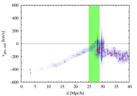
Figure 1: Peculiar velocities (line-of-sight component) in the direction of the supernova host galaxy, ESO 184$-$G82, as a function of the comoving distance from the Local Group formed the constrained simulation. The blue dots show dark matter particles and the red symbols represent dark matter haloes. The green band indicates the location of the galaxy ESO 184$-$G82.

SN 1998bw (Galama et al. 1998; Iwamoto et al. 1998; Kulkarni et al. 1998; Woosley et al. 1999) was the first SN discovered to be connected with a GRB (GRB 980425). It is the nearest GRB-SN so far, and the measured redshift is $z=0.00867\pm 0.00004$ (Foley et al. 2006), so it constitutes an important low-redshift anchor of the Hubble diagram. For the recessional velocity of this low-redshift system, the contribution from the peculiar velocity may be relatively substantial. The true recessional velocity $v_{\rm rec}$ due to the Hubble flow should be corrected for the peculiar velocity $v_{\rm pec}$ of the host galaxy: $v_{\rm CMB}=v_{\rm rec}+v_{\rm pec}$, with $v_{\rm CMB}$ being the velocity relative to the cosmic microwave background (CMB).

In order to estimate the peculiar velocity of its host galaxy, ESO 184$-$G82, and calculate the uncertainty in the distance modulus, we use a dark matter simulation performed as a part of the Constrained Local Universe Simulations (CLUES) project. The simulation is carried out in a volume of $(160h^{-1}{\rm Mpc})^{3}$ containing $1024^{3}$ particles. The assumed cosmological model is based on the 3rd data release of the WMAP satellite (WMAP3 cosmology), i.e., matter density $\Omega_{m}=0.24$, dimensionless Hubble parameter $h=0.73$, and normalization of the power spectrum $\sigma_{8}=0.76$. The initial conditions are generated from observational data of the galaxy distribution and galaxy velocities in the local universe (for technical details see Gottloeber et al. 2010). With this setup, the simulation recovers all observed structures on scales larger than $5h^{-1}{\rm Mpc}$. In particular, all nearby galaxy clusters and superclusters, such as the Virgo cluster, the Coma cluster, the Great Attractor and the Perseus–Pisces cluster, are well reproduced in the final simulation snapshot. On the other hand, small scale structures formed in the simulation emerge from a random realization of the power spectrum on these scales. Their evolution, however, is strongly constrained by nearby large-scale structures. Therefore, the simulation provides a realistic and dynamically self-consistent model for the matter distribution and the velocity field in the local universe.

The position vector of the host galaxy with respect to the Local Group in the simulation box can be found be matching angular separations from several large-scale structures. As the reference structures, we use the Coma cluster, the Perseus–Pisces cluster and the Great Attractor. Having determined the direction to the host galaxy from the Local Group in the simulation box, we compute the radial components of peculiar velocities within a narrow light cone. Figure 1 shows the resulting projected peculiar velocities as a function of the comoving distances from the Local Group. The blue dots show velocities of dark matter particles, whereas the red symbols represent dark matter haloes found with the friends-of-friends algorithm. Lack of dark matter haloes at small distances is related to the fact that the line of sight crosses the edge of the Local Void (see Nasonova & Karachentsev 2011).

To identify the position of the host galaxy ESO 184$-$G82 in the simulation box, we use a range of plausible distances to the host galaxy in units of Mpc/h so they are independent of $H_{0}$. We assume that the true recessional velocity is likely between the host velocity with respect to the CMB $v_{\rm CMB}=2505\pm 14$ km s^-1 (Foley et al. 2006) and the host velocity with respect to the local large-scale structures (Virgo, Great Attractor and Shapley Supercluster) $v_{\rm Virgo+GA+Shapley}=2769\pm 21$ km s^-1, as shown in the green band in Figure 1 . Within the green band, the mean peculiar velocity is $v_{\rm pec}=-65$ km s^-1 with a mean systematic error $\pm 75$ km s^-1. Combined with the peculiar velocity $v_{\rm pec}$ and the CMB velocity $v_{\rm CMB}$, the Hubble flow velocity is $v_{\rm rec}=2570\pm 76$ km s^-1, which is in the green band in Figure 1, as expected. The uncertainty of $v_{\rm pec}$ dominates the uncertainty of $v_{\rm rec}$. The corresponding redshift is $z=v_{\rm rec}/c=0.00857\pm 0.00025$. Therefore, the contribution of the peculiar velocity of the the host galaxy to uncertainty in the distance modulus of SN 1998bw is $\sigma({\rm DM})=(5/2.3)\sigma(v_{\rm pec})(cz)^{-1}=0.06$ mag, where $c$ is the speed of light and $\sigma(v_{\rm pec})$ is the uncertainty of peculiar velocity $v_{\rm pec}$.

3 GRB-SNE AS STANDARD CANDLES

In much the same way as SNe Ia were used to measure the cosmological parameters $\Omega_{m}$ and $\Omega_{\Lambda}$ (Perlmutter et al. 1997; Riess et al. 1998; Perlmutter et al. 1999), here we use GRB-SNe as standard candles.

Similar to SNe Ia (Phillips 1993; Phillips et al. 1999), GRB-SNe have bright peak luminosities. The luminosity-decline rate relation for GRB-SNe in the rest-frame V band is (Li & Hjorth 2014)

$$M_{\rm V,peak}=\alpha\Delta m_{V,15}+M_{0},$$ (1)

where $\alpha$ is the slope and $M_{0}$ is a constant representing the absolute peak magnitude at $\Delta m_{V,15}=0$. Assuming $\Omega_{m}=0.315$ and $H_{0}=67.3$ km s^-1 Mpc^-1 (Planck Collaboration et al. 2013), we have $\alpha=1.57^{+0.25}_{-0.28}$ and $M_{0}=-20.58^{+0.22}_{-0.20}$ (Li & Hjorth 2014). This relation is superior to other similar relations (Li & Hjorth 2014), such as the $k-s$ relation (Cano 2014), where $k$ and $s$ are the relative peak and width of the light curves compared to SN 1998bw, or the relation between the peak magnitude and the elapsed time since GRB. With $M_{\rm V,peak}$ from Li & Hjorth (2014), obtained using the above Planck cosmology, the corrected apparent peak magnitude in the rest-frame V band is

$$m_{V}^{\rm corr}=M_{\rm V,peak}+DM(z),$$ (2)

where $m_{V}^{\rm corr}$ is the corrected apparent magnitude in the rest-frame V band after corrections for dust extinction and K correction (Li & Hjorth 2014). Here $DM(z)$ is the distance modulus at $\Omega_{m}=0.315$ and $H_{0}=67.3$ km s^-1 Mpc^-1 in a flat universe. The values of $m_{V}^{\rm corr}$ are listed in Table 1. Considering the relation in Eq. (1), the effective apparent peak magnitude $m_{V}^{\rm eff}$ can be obtained as

$$m_{V}^{\rm eff}=m_{V}^{\rm corr}-\alpha\Delta m_{V,15}.$$ (3)

The term $\alpha\Delta m_{V,15}$ represents the correction due to the luminosity-decline rate relation. The effective apparent magnitude can also be expressed as (Perlmutter et al. 1997, 1999)

$$m_{V}^{\rm eff}=\Upsilon+5\log\mathcal{D}_{L}(z;\Omega_{m},\Omega_{\Lambda}),$$ (4)

where $\mathcal{D}_{L}\equiv H_{0}d_{L}$ is the “$H_{0}$-free” luminosity distance in units of km s^-1, with $d_{L}$ being the luminosity distance in units of Mpc (Hogg 1999) and $H_{0}$ in units of km s^-1 Mpc^-1. Here $\Upsilon=M_{0}-5\log H_{0}+25$ is the “$H_{0}$-free” V-band absolute peak magnitude (Perlmutter et al. 1997, 1999). The fitting procedure does not invoke $H_{0}$ and the constraints on cosmological parameters are therefore independent of the Hubble constant. In this paper, $\alpha$ and $\Upsilon$ are statistical ‘nuisance’ parameters.

4 CONSTRAINTS ON $\Omega_{m}$ and $\Omega_{\lambda}$

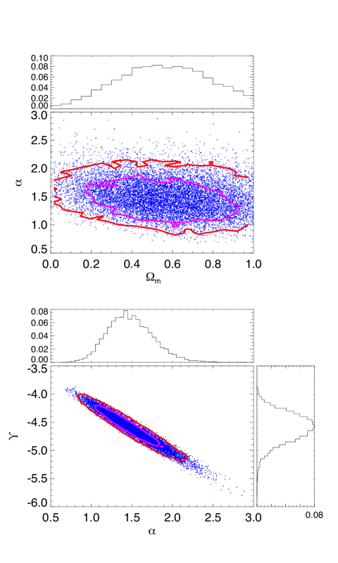
Figure 2: Constraints on $\alpha$, $\Upsilon$ and $\Omega_{m}$ assuming a flat cosmological model. The confidence levels of the density contours are 68.3% and 95.5%.

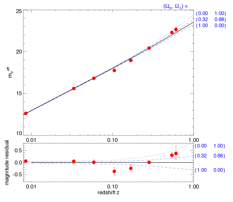
Figure 3: Hubble diagram for GRB-SNe. The effective apparent magnitudes of eight GRB-SNe plotted as red points, are calculated using the best-fit parameters $\alpha=1.37$ and $\Upsilon=-4.50$. The best cosmological model with $(\Omega_{m},\Omega_{\Lambda})=(0.58,0.42)$ is in black, while other models (labeled on the right side of the figure) are in blue. The lower panel shows the magnitude residuals from the best-fit cosmological model.

We employ a Monte Carlo Markov Chain technique to place constraints on the matter density parameters and the two nuisance parameters. We adopt a flat cosmological model, i.e. $\Omega_{m}+\Omega_{\Lambda}=1$, and assume a flat prior on all free parameters, i.e. $\Omega_{m}$, $\alpha$ and $\Upsilon$. With a straightforward generalization of the $\chi^{2}$ function from Astier et al. (2006), the adopted likelihood function $L$ is

$$L\propto\prod_{i}\exp\Big{[}\frac{\Delta_{i}^{2}}{2\sigma_{i}^{2}}\Big{]}\frac{1}{\sigma_{i}},$$ (5)

with $\Delta_{i}=m_{V,i}^{\rm corr}-\alpha\Delta m_{V,15,i}-\Upsilon-5\log\mathcal{D}_{L}(z_{i},\Omega_{m})$, where $\sigma_{i}^{2}=\sigma^{2}(m_{V,i}^{\rm corr})+\alpha^{2}\sigma^{2}(\Delta m_{V,15,i})$, and $\sigma(m_{V,i}^{\rm corr})$ and $\sigma(\Delta m_{V,15,i})$ are the errors of $m_{V,i}^{\rm corr}$ and $\Delta m_{V,15,i}$, respectively. The formula for $\sigma_{i}$ assumes an independent propagation of errors in $m_{V,i}^{\rm corr}$ and $\Delta m_{V,15,i}$. We verify this assumption by finding no signature of a correlation between $m_{V}^{\rm corr}$ and $\Delta m_{V,15}$ in a covariance matrix obtained from fitting the light curves.

The marginalised posterior probability densities of $\Omega_{m}$, $\alpha$ and $\Upsilon$ are shown in Figure 2. The confidence levels of the density contours are 68.3% and 95.5%. We quantify the fit in terms of the maximum-likelihood values and confidence intervals containing 68.3% of the corresponding marginal probabilities. The best-fit nuisance parameters are $\alpha=1.37^{+0.36}_{-0.19}$ and $\Upsilon=-4.50^{+0.17}_{-0.32}$, which are consistent with the values derived from the luminosity-decline rate relation, assuming $\Omega_{m}=0.315$ and $H_{0}=67.3$ km s^-1 Mpc^-1 (Li & Hjorth 2014). In a flat universe, the best-fit cosmological model is $(\Omega_{m},\Omega_{\Lambda})=(0.58^{+0.22}_{-0.25},0.42^{+0.25}_{-0.22})$.

Figure 3 shows the Hubble diagram for eight GRB-SNe systems. The effective magnitudes $m_{V}^{\rm eff}$ of the GRB-SN systems in the rest frame V band are plotted as red points. The best cosmological model is the black curve. For comparison, we plot three other cosmological models: {$(\Omega_{m},\Omega_{\Lambda})$} $=\{(0,1),(0.32,0.68),(1,0)\}$ as dotted lines. The lower panel in Figure 3 shows the magnitude residuals relative to the best cosmological model.

5 CONCLUSION

The cosmological parameters $\Omega_{m}$ and $\Omega_{\Lambda}$ can be constrained with SNe Ia (Perlmutter et al. 1999; Knop et al. 2003), CMB radiation (Spergel et al. 2003; Planck Collaboration et al. 2013), and clusters of galaxies (Allen et al. 2002; Jullo et al. 2010). As shown in this paper, GRB-SNe may add further constraints on cosmological parameters. With more systems at $z$ up to 1, the result would be more constraining, but we have opted here for systems with very well sampled light curves. At higher redshifts ($z>1.5$), with more powerful telescope to be launched, e.g., JWST, GRB-SNe are potential candidates to break the degeneracies and constrain the equation of state parameter $w(z)$ (Linder & Huterer 2003; King et al. 2013).

References

- Allen et al. (2002) Allen, S. W., Schmidt, R. W. & Fabian, A. C. 2002, MNRAS, 334, L11
- Astier et al. (2006) Astier, P., et al. 2006, A&A, 447, 31
- Cano (2014) Cano, Z. 2014, accepted by ApJ
- Drout et al. (2011) Drout, M. R., et al. 2011, ApJ, 741, 97
- Foley et al. (2006) Foley, S., Watson, D., Gorosabel, J., Fynbo, J. P. U., Sollerman, J., McGlynn, S., McBreen, B. & Hjorth, J. 2006, A&A, 447, 891
- Galama et al. (1998) Galama, T. J., et al. 1998, Nature, 395, 670
- Gottloeber et al. (2010) Gottloeber, S., Hoffman, Y., & Yepes, G. 2010, ArXiv e-prints
- Graur et al. (2014) Graur, O., et al. 2014, ApJ, 783, 28
- Hjorth (2013) Hjorth, J. 2013, Royal Society of London Philosophical Transactions Series A, 371, 20275
- Hjorth & Bloom (2012) Hjorth, J., & Bloom, J. S. 2012, The Gamma-Ray Burst - Supernova Connection, 169-190
- Hjorth et al. (2003) Hjorth, J., et al. 2003, Nature, 423, 847
- Hogg (1999) Hogg, D. W. 1999, ArXiv Astrophysics e-prints
- Hook (2013) Hook, I. M. 2013, Royal Society of London Philosophical Transactions Series A, 371, 20282
- Iwamoto et al. (1998) Iwamoto, K., et al. 1998, Nature, 395, 672
- Jullo et al. (2010) Jullo, E., Natarajan, P., Kneib, J.-P., D’Aloisio, A., Limousin, M., Richard, J., & Schimd, C. 2010, Science, 329, 924
- King et al. (2013) King, A. L., Davis, T. M., Denney, K., Vestergaard, M., & Watson, D. 2013, MNRAS, 441, 3454-3476
- Klebesadel et al. (1973) Klebesadel, R. W., Strong, I. B. & Olson, R. A. 1973, ApJ, 182, 85
- Knop et al. (2003) Knop, R. A., et al. 2003, ApJ, 598, 102
- Koekemoer et al. (2011) Koekemoer, A. M., et al. 2011, ApJS, 197, 36
- Kulkarni et al. (1998) Kulkarni, S. R., et al. 1998, Nature, 395, 663
- Li & Hjorth (2014) Li, X., & Hjorth, J. 2014, ArXiv e-prints
- Li et al. (2012) Li, X., Hjorth, J., & Richard, J. 2012, J. Cosmology Astropart. Phys, 11, 15
- Linder & Huterer (2003) Linder, E. V., & Huterer, D. 2003, Phys. Rev. D, 67, 081303
- Metzger et al. (1997) Metzger, M. R., Djorgovski, S. G., Kulkarni, S. R., Steidel, C. C., Adelberger, K. L., Frail, D. A., Costa, E., & Frontera, F. 1997, Nature, 387, 878-880
- Nasonova & Karachentsev (2011) Nasonova, O. G., & Karachentsev, I. D 2011, Astrophysics, 54, 1
- Pan & Loeb (2013) Pan, T., & Loeb, A. 2013, MNRAS, 435, 33
- Perlmutter et al. (1997) Perlmutter, S., et al. 1997, ApJ, 483, 565
- Perlmutter et al. (1999) Perlmutter, S., et al. 1999, ApJ, 517, 565
- Phillips (1993) Phillips, M. M., 1993, ApJ, 413, 105
- Phillips et al. (1999) Phillips, M. M., Lira, P., Suntzeff, N. B., Schommer, R. A., Hamuy, M., & Maza, J. 1999, AJ, 118, 1766
- Planck Collaboration et al. (2013) Planck Collaboration et al. 2013 , ArXiv e-prints
- Riess et al. (1998) Riess, A. G., et al. 1998, AJ, 116, 1009
- Rodney et al. (2014) Rodney, S. A., et al. 2014, AJ, 148, 13
- Schlafly et al. (2011) Schlafly, E. F., & Finkbeiner, D. P. 2011, ApJ, 737, 103
- Schlegel et al. (1998) Schlegel, D. J., Finkbeiner, D. P., & Davis, M. 1998, ApJ, 500, 525
- Spergel et al. (2003) Spergel, D. N., et al. 2003, ApJS, 148, 175
- Stanek et al. (2003) Stanek, K. Z., et al. 2003, ApJ, 591, 17
- Woosley & Bloom (2006) Woosley, S. E., & Bloom, J. S. 2006, ARA&A, 44, 507
- Woosley et al. (1999) Woosley, S. E., & Eastman, R. G. and Schmidt, B. P. 1999, ApJ, 516, 788