Tracing chemical evolution over the extent of
the Milky Way’s Disk with APOGEE Red Clump Stars

Abstract

We employ the first two years of data from the near-infrared, high-resolution SDSS-III/APOGEE spectroscopic survey to investigate the distribution of metallicity and $\alpha$-element abundances of stars over a large part of the Milky Way disk. Using a sample of $\approx 10,000$ kinematically-unbiased red-clump stars with $\sim$5% distance accuracy as tracers, the [$\alpha$/Fe] vs. [Fe/H] distribution of this sample exhibits a bimodality in [$\alpha$/Fe] at intermediate metallicities, $-0.9<$[Fe/H]$<-0.2$, but at higher metallicities ([Fe/H]$\sim$+0.2) the two sequences smoothly merge. We investigate the effects of the APOGEE selection function and volume filling fraction and find that these have little qualitative impact on the $\alpha$-element abundance patterns. The described abundance pattern is found throughout the range 5$<$$R$$<$11 kpc and 0$<$$|Z|$$<$2 kpc across the Galaxy. The [$\alpha$/Fe] trend of the high-$\alpha$ sequence is surprisingly constant throughout the Galaxy, with little variation from region to region ($\sim$10%). Using simple galactic chemical evolution models we derive an average star formation efficiency (SFE) in the high-$\alpha$ sequence of $\sim$4.5$\times$10^-10 yr^-1, which is quite close to the nearly-constant value found in molecular-gas-dominated regions of nearby spirals. This result suggests that the early evolution of the Milky Way disk was characterized by stars that shared a similar star formation history and were formed in a well-mixed, turbulent, and molecular-dominated ISM with a gas consumption timescale (SFE^-1) of $\sim 2$ Gyr. Finally, while the two $\alpha$-element sequences in the inner Galaxy can be explained by a single chemical evolutionary track this cannot hold in the outer Galaxy, requiring instead a mix of two or more populations with distinct enrichment histories.

1. Introduction

The Milky Way galaxy (MW) is a cornerstone in the study of the internal structure and evolution of large disk galaxies, because stellar populations in the MW can be studied using detailed observations of large samples of individual stars (e.g., Rix & Bovy, 2013). Over the past few decades these surveys have led to the discovery of disk stars at large distances above the plane through star counts (the thick disk; Yoshii 1982; Gilmore & Reid 1983), observations of abundance gradients over the extent of the disk (e.g., Audouze & Tinsley, 1976; Chen et al., 2003; Allende Prieto et al., 2006; Cheng et al., 2012; Boeche et al., 2014), and a detailed mapping of the local distribution of elemental abundances (e.g., van den Bergh, 1962; Fuhrmann, 1998; Adibekyan et al., 2012). In addition, the first year of high-resolution spectroscopy from the Sloan Digital Sky Survey III’s Apache Point Observatory Galactic Evolution Experiment (APOGEE) was used by Hayden et al. (2014) and Anders et al. (2014) to study the Milky Way’s disk over a large area. These measurements provide crucial constraints on models for the formation and evolution of the MW disk (e.g., Larson, 1976; Chiappini et al., 1997). In this paper we extend these observations by tracing the detailed distribution of elemental abundances of red clump stars over a large part of the MW’s disk using the first two years of APOGEE data.

In the solar neighborhood, the distribution of stars in the ([$\alpha$/Fe],[Fe/H]) plane displays a sequence extending from metal-poor, high-$\alpha$ stars to about solar abundances that is believed to be associated with the thick disk, because of the large velocity dispersion of its stars (Fuhrmann, 1998; Prochaska et al., 2000; Bensby et al., 2005; Reddy et al., 2006; Ramírez et al., 2007; Lee et al., 2011). This sequence was originally established by observing stars kinematically selected to be likely members of a thick-disk population; this kinematical bias has made the interpretation of this sequence, its precise relation to the thick disk, and its extension to solar abundances difficult (e.g., Bensby et al., 2007). Recently, the kinematically-unbiased HARPS sample (Adibekyan et al., 2012) has removed this obstacle, and demonstrated that the high-$\alpha$ stars extend to solar and super-solar metallicities (Adibekyan et al. 2011, 2013; see also Bensby et al. 2014). The stars in this high-$\alpha$ sequence have ages of $\sim$7 Gyr and larger (Haywood et al., 2013), with more $\alpha$-enhanced objects being older, with ages up to 12 Gyr (Bensby et al., 2005). The spread in age and [$\alpha$/Fe] for stars in the thick disk indicates an extended star-formation history with time for enrichment by Type Ia supernovae (a few Gyr; Maoz et al. 2011).

Recently, progress has been made in mapping the spatial distribution of chemically differentiated stellar populations in the disk. In particular, it has become clear that high-$\alpha$ stars have a shorter radial scale length than stars with solar [$\alpha$/Fe] (Bensby et al., 2011a; Bovy et al., 2012b; Cheng et al., 2012; Anders et al., 2014). Bovy et al. (2012b) mapped the spatial distribution (scale height and length) of different mono-abundance populations in detail, finding a complex dependence of the radial scale length on ([$\alpha$/Fe],[Fe/H]), a smooth distribution of scale-heights ranging between 200 pc and 1 kpc, and a similarly smooth increase of the velocity dispersion with [$\alpha$/Fe] (Bovy et al. 2012a, c; see also Haywood et al. 2013). After accounting for the spatial selection function of SEGUE, Bovy et al. find a smooth distribution in the ([$\alpha$/Fe],[Fe/H]) plane at the solar cylinder, finding no distinct gap along the high-$\alpha$ sequence seen in other studies (e.g., Fuhrmann, 1998; Reddy et al., 2006; Adibekyan et al., 2011). This behavior can be interpreted as showing that the scale-height of the MW disk continuously and gradually decreased over time as the disk was enriched with metals, while the [$\alpha$/Fe] abundances decreased (due to Type Ia supernovae becoming the dominant form of enrichment). The complicated radial behavior of different mono-abundance populations—with the short scale lengths for the high-$\alpha$ stars, longer scale lengths for stars with solar abundances, and almost constant radial densities for low-$\alpha$, low-[Fe/H] stars—means, however, that it is difficult to extrapolate the local abundance distribution in order to further constrain the radial profiles. It is therefore essential to trace the ([$\alpha$/Fe],[Fe/H]) distribution over a much wider range of Galactocentric radii to obtain a full picture of the large-scale chemical structure of the disk.

Various qualitatively different scenarios for the formation of the thick, old, high-$\alpha$ component in the MW have been suggested since the result was first identified by Yoshii (1982) and Gilmore & Reid (1983). Many of these ideas were proposed in the first decade after the discovery and were reviewed by, for example, Majewski (1993). Some of these mechanisms rely on external events such as satellite heating, accretion, or merger-induced star formation (e.g., Abadi et al., 2003; Quinn et al., 1993; Brook et al., 2004), while others rely on internal evolution of the disk through slow or more rapid dissipational collapse during disk formation (Larson, 1976; Gilmore, 1984) or secular disk heating. A qualitatively new thick-disk formation scenario, suggested more recently, is stellar radial migration via spiral wave scattering at corotational resonance (Sellwood & Binney, 2002). Schönrich & Binney (2009b) suggested that this mechanism is able to produce a thick-disk component in agreement with many local observations, although more realistic simulations cast serious doubt on whether radial migration can produce enough (Roškar et al., 2013) or even any (Minchev et al., 2012b; Vera-Ciro et al., 2014b) heating. The results of Bovy et al. (2012b) disfavor an external origin for the thick disk, and find that the local observations can be reproduced by models where radial migration plays a large role. However, the observations can also be explained by models where the thick disk formed largely as it is seen today, from a hot interstellar medium at the onset of disk formation, as favored by recent cosmological simulations (e.g., Bird et al., 2013; Stinson et al., 2013) and observations of high-mass disk galaxies at $z\approx 2$ (e.g., Förster Schreiber et al., 2011), or by a combination of early merging with radial migration (Minchev et al., 2013). A detailed mapping of the chemical structure of the disk away from the solar neighborhood will allow insights into the evolution of different regions of the MW and provide qualitatively new constraints on the evolutionary models described above.

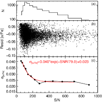
Figure 1.— The scatter in [$\alpha$/Fe] of the low-$\alpha$ sequence of stars ([$\alpha$/Fe]$<$$+$0.10; see Figure 10) with $S/N$ after subtraction of the trend of [$\alpha$/Fe] with metallicity (i.e., the “banana” shape). (a) Histogram of low-$\alpha$ stars in each (logarithmic) bin of $S/N$. (b) The residual [$\alpha$/Fe], after subtraction of the low-$\alpha$ [$\alpha$/Fe] trend with [Fe/H], versus $S/N$. (c) $\sigma_{\rm[\alpha/Fe]}$, the robust standard deviation of the residual [$\alpha$/Fe] in logarithmic bins of $S/N$, versus $S/N$ showing an exponential decline with $S/N$. The scatter reaches a plateau of 0.023 dex at $S/N$$\gtrsim$300. The red line shows an exponential fit to the $\sigma_{\rm[\alpha/Fe]}$ values.

The relationships between various elemental-abundance groups and between abundances and age hold important clues about the evolution of the various stellar populations constituting the MW disk. High-resolution spectroscopic surveys, in combination with astrometry from Gaia (de Bruijne, 2012) and high-precision asteroseismology data, will allow these relations to be investigated over a much larger volume of the disk than the local solar neighborhood, which has been the focus of past surveys. Anders et al. (2014) studied the [$\alpha$/Fe] vs. [Fe/H] distribution of red giants in three radial bins using the first year of APOGEE data. In this paper we go beyond this analysis by employing a sample of $\approx 10,000$ red clump stars with accurate distances from the first two years of the APOGEE survey to investigate in detail the relation between [$\alpha$/Fe] and [Fe/H] over a large part of the MW disk using a large, statistical sample of stars spanning a wide range of ages and a proper accounting for the targeting selection effects. This unique sample allows tracing of the locally-observed high- and low-$\alpha$ sequences toward and away from the Galactic center, and to multiple kiloparsecs above the plane.

This paper is organized as follows. In Section 2 we discuss the APOGEE observations and data reduction, and we describe the sample of red clump (RC) stars and biases pertaining to its selection in Section 3. Our results are presented in Section 4. Chemical evolution models are discussed in Section 5.1, and the significance of our results is presented in Section 5.

In this study, we use Galactocentric rectangular coordinates (X,Y,Z) and left-handed Galactocentric cylinderical coordinates (R,Z,$\phi$), assuming that the Sun is 25 pc above the midplane and 8 kpc from the Galactic center, as in the APOGEE–RC catalog paper (Bovy et al., 2014).

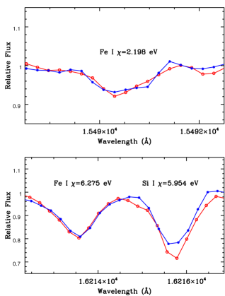
Figure 2.— Selected spectral lines from Fe I and Si I (an $\alpha$-element) in the two red clump stars with different [$\alpha$/Fe] values used in the manual analysis. In both 2M15152520+0102019 (red, $\alpha$-enhanced) and 2M06054047+2708560 (blue, solar-$\alpha$) the two Fe I lines have identical strengths, while the Si I line is significantly stronger in 2M06054047+2708560. Two Fe I lines are shown, with one being low excitation and the other having a high excitation energy; the fact that both lines have the same strength in both stars indicates that (1) their effective temperatures are very similar and (2) they have nearly the same Fe abundance. The stronger Si I line in 2M15152520+0102019 shows that it is $\alpha$-enhanced relative to the near-same Fe-abundance red clump star 2M06054047+2708560.

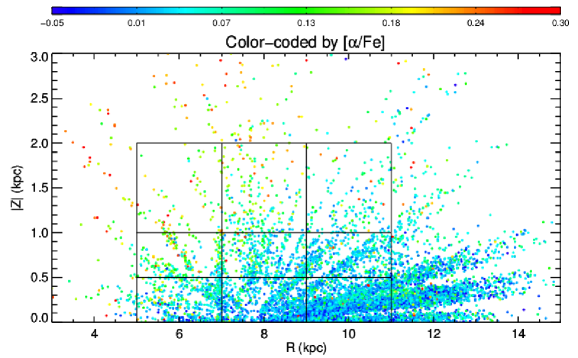
Figure 3.— $|Z|$ vs. $R$ distribution of APOGEE RC stars color-coded by [$\alpha$/Fe]. The nine $R/Z$ boxes used in Figure 11 are shown.

2. Observations And Data Reduction

We use the SDSS-III/APOGEE year 1 and 2 data for our analysis. The APOGEE survey is described in Eisenstein et al. (2011) and Majewski et al. (2014, in preparation), and the instrument in Wilson et al. (2010, 2012). The data reduction is briefly described in Nidever et al. (2012), and will be described in more detail in the near future (D. Nidever et al. 2014, in preparation). Stellar parameters are derived for each star using a $\chi^{2}$ optimization algorithm with a large, custom-built library of synthetic spectra (Allende-Prieto et al., 2014, A. E.  García Pérez et al. 2014, in preparation). Pipeline versions similar to those used for Data Release 10 (Ahn et al., 2014) were also used for the year 1 and 2 data that are the basis for this analysis. The APOGEE pipelines produce reduced spectra, accurate radial velocities ($\sigma_{\rm RV}$$\sim$$0.1$ km s${}^{-1}~{}$for most stars), and stellar parameters that have been calibrated using globular clusters and other “standards” (Mészáros et al., 2013). In the APOGEE synthetic spectral library the $\alpha$ elements O, Mg, Si, S, Ca, and Ti are varied together in the $\alpha$ dimension of the 6-dimension grid. Although the ASPCAP derived [$\alpha$/Fe] abundance from the best-fit $\chi^{2}$ solution can often be thought of as the “mean” abundance of these $\alpha$ elements, we find that in the limited $T_{\rm eff}$ and $\log{g}$ range of the RC sample the elements O, Mg and Si are dominant.

The $H$-band has only recently been explored for high-resolution spectroscopy of late-type stars, and, therefore, detailed line formation studies in non Local Thermodynamical Equilibrium (LTE) for this window and these stars are not available. Departures from LTE are always a concern in an analysis based on classical model atmospheres and LTE line formation (i.e., assuming the source function is equal to the Planck function). Specific calculations for each ion of interest are needed to solve this issue. However, departures from LTE tend to be reduced when the radiation field is weak (e.g., atmospheres of cool stars) and the density is high (i.e., dwarf stars). In our case we deal with cool stars with low gravities, and therefore some caution is advised.

We should note that working in the $H$-band, right at the intersection where H^- bound-free opacity yields to H^- free-free opacity at about 1.6 $\mu$m, the total opacity reaches a minimum for cool stars. This causes the continuum to form in deeper atmospheric layers, and so do absorption lines, which tend to be weak and in general form not too far from the layers where the continuum forms. The higher density in those layers, compared to those the optical spectrum is sensitive to, favors the assumption of LTE. At low metallicity, the lack of free electrons makes it hard to couple matter with the radiation field. Nonetheless, lower metallicities bring higher pressure and an increased role of collisions with hydrogen atoms. Unfortunately, the collisional rates associated with inelastic hydrogen collisions are set on firm theoretical basis only for a few of the lightest ions (Belyaev & Barklem, 2003; Belyaev et al., 2010; Barklem et al., 2012).

While the APOGEE [$\alpha$/Fe] abundances have not been thoroughly calibrated, an initial comparison of the [$\alpha$/Fe] abundances for stars with literature values indicates that the APOGEE [$\alpha$/Fe] values are in line with expectations. There are some peculiarities in the [$\alpha$/Fe] abundances for cool stars ($T_{\rm eff}$ $\lesssim$4200 K), that are generally difficult to analyze, but these effects are not apparent for warmer stars, including our RC sample. Indeed, for the stellar parameters typical of RC stars, the differences between the best-fit APOGEE spectra and those obtained with spherical MARCS models (Gustafsson et al., 2008) and Turbospectrum (e.g., Plez, 2012) are below 5%. The external uncertainties for [Fe/H] are $\sim$0.1 dex and $\sim$0.05 for [$\alpha$/Fe], although these decrease with metallicity and are roughly $\sim$0.03–0.04 ([$\alpha$/Fe]) and $\sim$0.02–0.07 ([Fe/H]) for the metallicities we consider here ($-0.9<$[Fe/H]$<+0.5$) (Mészáros et al., 2013). Figure 1 shows the empirical scatter in [$\alpha$/Fe] for the low-$\alpha$ group ([$\alpha$/Fe]$<$0.10, $5\lesssim$$R$$\lesssim 15$ kpc, $Z$$\lesssim$3 kpc, see Figure 10 below) around the [$\alpha$/Fe] trend with [Fe/H] (the “banana” shape) as a function of $S/N$. This scatter indicates the level of internal precision and decreases exponentially with $S/N$, reaching a plateau of $\sim$0.025 dex for $S/N$$\gtrsim$200; $\sigma_{\rm[\alpha/Fe]}=0.040$ $\exp(-SNR/79.0)+0.023$. The mean precision of all RC stars based on the exponential fit is $\sim$0.027. It is likely that the plateau in $\sigma_{\rm[\alpha/Fe]}$ at high $S/N$ is due to systematic effects in the spectra or abundances, and indicates that the astrophysical scatter of stars in this sequence is below $\sim$0.02 dex.

$\begin{array}[]{cc}\includegraphics[angle={0},scale={0.40}]{f4a.pdf}\includegraphics[angle={0},scale={0.40}]{f4b.pdf}\end{array}$

Figure 4.— (left) The selection function fraction (SFFRAC) for all APOGEE stars in the statistical sample. (right) The mean selection function in the $R-|Z|$ plane for the RC stars (logarithmic scale).

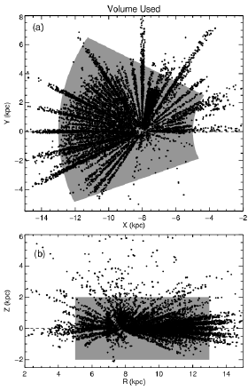
Figure 5.— The portion of the Galaxy explored by the APOGEE RC stars (solid dots); X–Y in (a) and $R$–$Z$ in (b). The gray shading indicates the region for which the volume correction is calculated in Section 3: 5 $\leq$ $R$ $\leq$ 13 kpc, $-$2 $\leq$ $Z$ $\leq$ $+$2 kpc, and $-$22${}^{\circ}~{}$$\leq$ $\phi$ $\leq$ $+$30°.

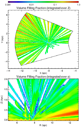
Figure 6.— The volume filling fraction in the (a) X-Y, and (b) $R-|Z|$ planes (logarithmic scales).

2.1. Manual Consistency Check

As a straightforward test of the ability of ASPCAP to differentiate stars having different [$\alpha$/Fe] values, two RC stars with $S/N$$\approx$100 were chosen to be subjected to a manual abundance analysis: 2M15152520+0102019 and 2M06054047+2708560. These two stars were found to have very similar stellar parameters by ASPCAP (with typical RC values), but differing [$\alpha$/Fe] values. In the case of 2M15152520+0102019, ASPCAP finds $T_{\rm eff}$= 4891K, $\log{g}$ = 2.65, [Fe/H]= $-$0.46, and [$\alpha$/Fe]= $+$0.33. The other star, 2M06054047+2708560, has ASPCAP values of $T_{\rm eff}$= 4895K, $\log{g}$ = 2.64, [Fe/H]= $-$0.45, and [$\alpha$/Fe]= $-$0.03.

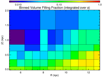
Figure 7.— The binned volume filling fraction in the $R-|Z|$ plane (logarithmic scale).

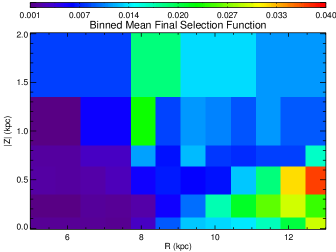
Figure 8.— The binned mean final selection function in the $R-|Z|$ plane (linear scale).

Model atmospheres from the same grid (ATLAS9, scaled-solar abundance models) as that used for ASPCAP were interpolated, and an LTE abundance analysis using the spectrum synthesis code MOOG was carried out for the elements iron, magnesium, silicon, calcium, and titantium. The spectral lines chosen to be synthesized were those listed in Smith et al. (2013), who explored spectral windows for various elements using the APOGEE wavelength range and APOGEE linelist in an analysis of field red giant standard stars. The elements Mg, Si, Ca, and Ti are taken to represent the $\alpha$-elements. As ASPCAP in its current form averages the abundances of the $\alpha$-elements together to form a single [$\alpha$/Fe] index, the same average is computed here. Synthesis of the Fe I, Mg I, Si I, Ca I, and Ti I lines was carried out for both RC stars as done in Smith et al. (2013), and the results for each element are now noted for each star. For 2M15152520+0102019 the abundances are: [Fe/H]= $-$0.44$\pm$0.09, [Mg/H]= $-$0.24$\pm$0.15, [Si/H]= $-$0.26$\pm$0.07, [Ca/H]= $-$0.17$\pm$0.03, and [Ti/H]= $-$0.15$\pm$0.02, leading to [$\alpha$/Fe]= $+$0.24$\pm$0.10. For 2M06054047+2708560 the abundances are: [Fe/H]= $-$0.48$\pm$0.11, [Mg/H]= $-$0.36$\pm$0.18, [Si/H]= $-$0.44$\pm$0.07, [Ca/H]= $-$0.48$\pm$0.04, and [Ti/H]= $-$0.57$\pm$0.04, which then yields [$\alpha$/Fe]= $+$0.02$\pm$0.12.

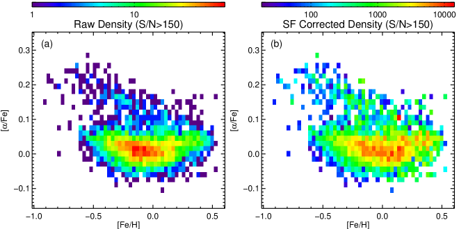
Figure 9.— The effect of the selection function on the abundance patterns in the [$\alpha$/Fe] vs. [Fe/H] plane. (a) The raw density of RC stars, and (b) the selection function corrected density of RC stars.

The manual analysis confirms the ASPCAP result that both RC stars have similar Fe abundances, while 2M15152520+0102019 is $\alpha$-enhanced and 2M06054047+2708560 has a [$\alpha$/Fe] value that is solar. The differences between these two stars is illustrated visually in Figure 2, where selected Fe I and Si I lines are over-plotted for the two stars. Both stars have near-identical Fe I lines (both low-excitation and high-excitation energies), with 2M15152520+0102019 exhibiting a significantly stronger Si I line, resulting in a larger Si abundance in this star. Similar differences are found in the Mg I, Ca I, and Ti I lines, demonstrating that 2M15152520+0102019 has an elevated value of [$\alpha$/Fe]. The ASPCAP abundances are very similar to those provided by the manual analysis: for 2M15152520+0102019 $\Delta$[Fe/H](ASPCAP$-$Manual) = $-$0.02 dex, while 2M06054047+2708560 has $\Delta$[Fe/H](ASPCAP$-$Manual) = $+$0.03 dex. In the case of the ratios of [$\alpha$/Fe], 2M15152520+0102019 has $\Delta$[$\alpha$/Fe](ASPCAP$-$Manual) = $+$0.09 dex and 2M06054047+2708560 has $\Delta$[$\alpha$/Fe](ASPCAP$-$Manual) = $-$0.05 dex. In all abundances and their ratios, the differences are $\lesssim$ 0.1 dex (i.e., less than the measurement uncertainties of the manual analysis), and indicate that ASPCAP is deriving reliable stellar parameters, metallicities, and mean $\alpha$-to-Fe ratios for RC stars. A more detailed analysis of ASPCAP abundance uncertainties will be presented in A. E. García Pérez et al. (2014, in preparation).

3. Sample and Selection Effects

For this analysis we use the He-core burning red clump stars observed by APOGEE. RC stars are in general $\sim$3–4 times more numerous than stars on the upper red giant branch (RGB, brighter than the RC). Due to APOGEE’s simple targeting color cuts, ($J$-$K_{\rm s}$)₀$>$0.5, many RC stars have been observed by APOGEE (Zasowski et al., 2013). An advantage conferred by use of RC stars for a spatial survey of stars is that their absolute magnitudes vary little with age and metallicity (Girardi et al., 2002; Groenewegen, 2008), i.e., they are “standard candles”, and their distances can be readily and reliably inferred. The RC stars also have the added benefit of being warm enough that their APOGEE [$\alpha$/Fe] abundances are reliable and don’t suffer from systematic effects currently seen in the APOGEE abundances of cool giants (Anders et al., 2014; Hayden et al., 2014).

The RC sample selection is described in detail in our companion paper on the APOGEE–RC catalog (Bovy et al., 2014). In brief, we select RC stars using simple selections in $\log{g}$ as a function of $T_{\rm eff}$, and in dereddened color as a function of metallicity. A comparison with APOGEE stars that have accurate surface-gravity measurements from Kepler astroseismology (M. Pinsonneault et al. 2014, in preparation) demonstrates that our RC sample suffers $\lesssim$7% “contamination” from RGB stars. The RC $K_{\rm s}$-band magnitudes are extinction-corrected using 2MASS+$Spitzer$/WISE photometry and the RJCE method (Majewski et al., 2011). PARSEC models (Bressan et al., 2012) are employed to determine the absolute magnitude of the RC stars using ([Fe/H],[J-K_s]₀). The derived RC distances are accurate to $\sim$5%. The majority of RC stars are within $\sim$4–5 kpc from the sun, but some extend out to $\sim$10 kpc. The final catalog has 10,341 RC stars and their distribution in the $|$Z$|$–$R$ plane is shown in Figure 3.

$\begin{array}[]{cc}\includegraphics[angle={0},scale={0.40}]{f10a.pdf}\includegraphics[angle={0},scale={0.40}]{f10b.pdf}\end{array}$

Figure 10.— (left) The [$\alpha$/Fe] vs. [Fe/H] diagram for our sample of APOGEE RC stars with $S/N$$>$150 (3954 stars). The bimodality in [$\alpha$/Fe] at low [Fe/H] is clearly visible and extends over $\sim$0.6 dex in metallicity. The error bar in the lower left corner shows representative precisions of 0.05 dex in [Fe/H] and 0.027 dex in [$\alpha$/Fe]. (right) A schematic of our RC [$\alpha$/Fe] vs. [Fe/H] diagram showing the main features: the low-$\alpha$ group (red), high-$\alpha$ group (blue), and intermediate-$\alpha$ “valley”. The hashed red/blue shows the overlap region between the low- and high-$\alpha$ stars. The black dots are RC stars with $S/N$$>$150.

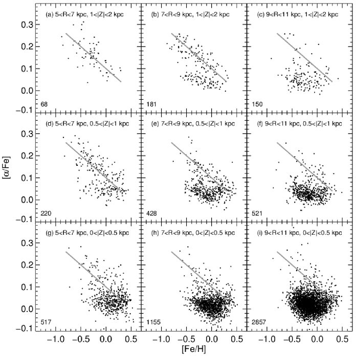
Figure 11.— The [$\alpha$/Fe] vs. [Fe/H] diagram of our RC stars, similiar to Figure 10, but now separated into nine different Galactic $R$ and $Z$ zones. A high-$\alpha$ sequence fiducial gray line, [$\alpha$/Fe]=$-$0.2$\times$[Fe/H]$+$0.10, is drawn in all the panels. The number of stars in each spatial zone is shown in the bottom left corner.

The APOGEE targeting scheme is described in detail in Zasowski et al. (2013). There are three main selection effects introduced by the targeting scheme used by APOGEE:

1. The color cut of ($J$-$K_{\rm s}$)₀$>$0.5. This removes RC stars with [Fe/H]$<-0.9$, but only marginally affects our results because most MW disk stars are more metal-rich than this cutoff (see Section 5 of Bovy et al. 2014).

2. The magnitude groups or “cohorts”. APOGEE targets are selected in three magnitude ranges: 7$<$$H$$<$12.2 (short), 12.2$<$$H$$<$12.8 (medium), and 12.8$<$$H$$<$13.3/13.8 (long) with 3/6/12–24 “visits” per group respectively to attain net $S/N$=100 for stars in each group. Each magnitude range is divided into three magnitude bins with equal numbers of stars and then 1/3 of the stars allocated for that magnitude range are randomly drawn from each of the three bin (see Zasowski et al. 2013 for more details). Because the brighter stars reach their $S/N$ threshold more quickly, multiple groups of stars, or cohorts, are observed in that range over the many visits to that field. Due to this scheme, a larger number of brighter (closer) stars are observed than fainter (distant) stars. In general, the 230 science fibers allocation by cohort is roughly 90/90/50, although this distribution varies with $l$ and $b$.

3. The placement of fields in the sky. APOGEE uses a fairly uniform grid of fields in Galactic ($l$,$b$), as seen in Zasowski et al. (2013) and the left panel of Figure 4.

The effects from (2) and (3) create spatial biases in the APOGEE sampling of the RC stars across the MW. However, the selection bias is only in apparent magnitude, and, because RC stars are standard candles within $\sim$0.05 mag, the bias is in RC distance and the Galactic coordinates $R$ and $Z$. If the abundances of stars vary with position in the Galaxy, which has been shown by previous studies (e.g., Cheng et al., 2012; Bovy et al., 2012a; Schlesinger et al., 2012; Anders et al., 2014; Hayden et al., 2014; Boeche et al., 2014), this positional bias can create a chemical bias. If, however, the analysis is restricted to small positional zones, or the abundances explicity plotted with their dependence on position, then the bias is effectively removed.

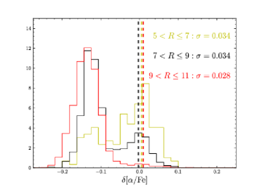
Figure 12.— The deviation of stars from the high-$\alpha$ trend line, $\delta$[$\alpha$/Fe] vs. [$\alpha$/Fe]. Stars with $S/N$$>$70, $|Z|$$\leq$3 kpc, $-0.6$$\leq$[Fe/H]$\leq$$-0.2$ are used in three radial bins. The trend line is $-0.2\times$[Fe/H]$+0.10$.

We correct for the APOGEE selection effects in two steps: (1) the stars in our fields that could have been observed but were not, and (2) the survey coverage or volume correction, i.e., stars in fields that we did not observe. The first step is fairly straightforward, and is described in detail in $\S$4 of the RC catalog paper. For every adopted target selection cut we count the number of stars that passed the cut and compare this number to the actual number of stars observed by APOGEE for this field; the ratio (N_observed/N_total) is the selection function fraction (SFFRAC) for these APOGEE-observed stars. In our disk and bulge fields, there is a simple ($J$-$K_{\rm s}$)₀$>$0.5 color cut and magnitude limits for the cohorts. However, in the halo fields, supplemental Washington M, T₂ and DDO51 (W+D; Majewski et al., 2000) photometry was often used to pre-select giant stars (Zasowski et al., 2013). The target selection in these fields included whether 2MASS-detected stars were identified as giants based on the W+D photometry and was therefore more complex. However, the method for calculating the selection effects remains the same. The selection function fraction was computed for stars in all fields that were selected as part of the APOGEE “survey” or “statistical” (as it is referred to in the RC catalog paper) sample (i.e., not Kepler fields, ancillary targets, globular cluster members, etc.). The left panel of Figure 4 shows the SFFRAC in the APOGEE fields explored here (year 1+2). The SFFRAC values are low for the low-latitude fields (especially in the inner galaxy) because there are far so many thin disk stars that could be targeted according to the color and magnitude selection criteria. The opposite is seen in the higher-latitude ($|$b$|$$>$16°), “halo” fields where the values are high because the overall density of stars is low and all possible stars are observed. The right panel of Figure 4 shows the mean SFFRAC of the RC stars in the $R-|Z|$ plane.

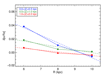
Figure 13.— The median $\delta$[$\alpha$/Fe] (deviation from the high-$\alpha$ trend line) for high-$\alpha$ stars ([$\alpha$/Fe]$>$0.09) separated for our nine $R/Z$ zones (as seen in Figure 11) versus $R$ with zones at the same $|Z|$ connected by lines (and color-coded). Dashes lines show the best-fit linear trend of $\delta$[$\alpha$/Fe] with $R$ for the three zones at the same $|Z|$. There is a negative gradient of $\delta$[$\alpha$/Fe] with $R$ at any $|Z|$ with a slope that decreases with $|Z|$.

The second step is to calculate the fraction of the Galactic volume that is explored with the APOGEE RC stars we actually did probe as a function of $R-|Z|$. We calculate a fine grid (steps of 20 pc in $R$/$Z$ and 0.2${}^{\circ}~{}$in $\phi$) in Galactic cylindrical coordinates for the region explored by the APOGEE RC stars: 5 $\leq$ $R$ $\leq$ 13 kpc, $-$2 $\leq$ $Z$ $\leq$ $+$2 kpc, and $-$22${}^{\circ}~{}$$\leq$ $\phi$ $\leq$ $+$30${}^{\circ}~{}$(gray region in Figure 5). We then flag every voxel (pixel in our 3D grid) that falls within the cone of one of the APOGEE survey fields. The volume filling fraction in the X-Y (integrated over $Z$) and $R-|Z|$ (integrated over $\phi$) planes are shown in Figure 6. These values show the opposite trends of SFFRAC. APOGEE covers a large fraction of the volume in the midplane but a significantly lower fraction at high latitude. However, there are hardly any holes in the $R-|Z|$ plane except for a few gaps at high-latitude in the inner galaxy. To correct for these missed regions we bin the volume fractions in the $R-|Z|$ plane with zones of $\sim$45 stars or more (Figure 7). All RC stars in the above-mentioned volume are given volume correction fractions based on the binned image.

The product of the two selection functions, SFFRAC and the volume filling fraction, is taken to produce the final selection function as seen in Figure 8 (on a linear scale). These values show some variations in the $R-|Z|$ plane but they are not large and vary smoothly with position. To assess the impact of the APOGEE selection function on the abundance patterns in the [$\alpha$/Fe] vs. [Fe/H] plane, we compare the raw density to the selection function corrected density (each star weighted by the inverse of the final selection function) of RC stars seen in Figure 9. The selection function correction changes the relative numbers of stars in each abundance group but the overall pattern of abundances does not change. This effect is especially clear when comparing to the unbinned plot in the left panel of Figure 10. Because in this paper we are focused on the patterns in the abundance plane and information is lost by binning, we use the raw scatter plots for the rest of the paper.

4. Results

4.1. Full Sample

Figure 10 displays the [$\alpha$/Fe] vs. [Fe/H] diagram for all of our APOGEE RC stars with $S/N$$>$150. The $\alpha$-bimodality is clearly visible for $-0.9<$[Fe/H]$<-0.2$ dex. Our $\alpha$-element abundance distribution shows some differences compared to the medium-resolution SEGUE G-dwarf sample of Lee et al. (2011) and Bovy et al. (2012b), especially in the distinct bimodality at the metal-poor end. In the APOGEE RC sample, both high- and low-$\alpha$ groups are quite extended in [Fe/H], and the bimodality is seen over $\sim$0.5 dex of metallicity. In contrast, the two $\alpha$ groups in the SEGUE studies extend over smaller ranges in metallicity, with a quick transition from high- to low-$\alpha$ and no clear bimodality at the metal-poor end. This difference is likely due to higher uncertainties in the SEGUE data, and their lack of low-latitude fields (the distribution of Cheng et al. 2012, which include some low-latitude SEGUE fields, looks qualititatively more similar to our RC data). The APOGEE distribution compares well to those of other high-resolution studies (e.g., Fuhrmann, 2011; Bensby et al., 2014), most notably the HARPS sample of local stars (most within $\sim$45 pc; Adibekyan et al., 2013) as shown by Anders et al. (2014, see their Figure 9), although our sample is $\sim$10 times larger, and extends to significantly larger distances.

We identify four main qualitative features of our RC [$\alpha$/Fe] vs. [Fe/H] diagram, which are labeled in the schematic (Figure 10 right panel):

1. $\alpha$ Bimodality: In the metallicity range $-0.9<$[Fe/H]$<-0.2$ the high and low-$\alpha$ groups are well separated by a less populated chemical region.

2. The two $\alpha$ groups converge at high metallicity, [Fe/H]$\sim+$0.2. This feature has also been seen in other recent high-resolution studies (e.g., Adibekyan et al., 2013; Ramírez et al., 2013; Bensby et al., 2014; Recio-Blanco et al., 2014; Bergemann et al., 2014). At high metallicities and low [$\alpha$/Fe], where the two groups merge, it is not completely clear how to associate stars with the two groups and we, therefore, show this as a hashed red/blue region in the figure.

3. The region between the $\alpha$ groups is not completely empty. Stars exist there, but at lower densities than the high/low-$\alpha$ regions. This statement is still true when examining the selection function corrected abundances (Figure 9) and the highest $S/N$ stars; which should have low scatter from abundance uncertainties.

4. The solar-$\alpha$ group extends over $\sim$1 dex of metallicity ($-0.6<$[Fe/H]$<+0.5$) and has a “banana” shape. This shape is seen in previous studies such as the [Ti/Fe] abundances in Bensby et al. (2014, their Figure 15.).

The clear [$\alpha$/Fe] bimodality in the APOGEE data was first shown by Anders et al. (2014) using the first year data, and we confirm this result with our cleaner red clump sample and find that it is not caused by selection effects (Figure 9).

4.2. Spatial Variations

Figure 11 shows the [$\alpha$/Fe] vs. [Fe/H] diagram for our RC stars broken into nine regions in R and $|$Z$|$. The selection effects have a minor effect in these small spatial regions. The same general patterns are seen in these panels as were noted in Figure 10 of all stars, except that the relative contributions of subpopulations vary. Panels (b), (d) and (e) show the bimodality most prominently.

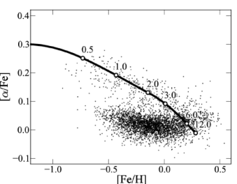
Figure 14.— The fiducial GCE model for the high-$\alpha$ sequence with SFE=$\sim 4.5\times 10^{-10}\,{\rm yr}^{-1}$. The labeled open circles indicate the abundance of each model at the given time in Gyr.

The high-$\alpha$ stars lie close to the fiducial gray line (in all panels). Figure 12 shows $\delta[\alpha$/Fe] (which is [$\alpha$/Fe] minus the fiducial line) for stars with $S/N$$>$70, $|Z|$$\leq$3 kpc, and $-0.6$$\leq$[Fe/H]$\leq$$-0.2$ in three Galactic radial bins. A two-Gaussian fit was performed for each radius, and the means of the Gaussian around $\delta[\alpha$/Fe]=0 are shown as dashed lines. The means are nearly identical, which suggests that the high-$\alpha$ stars fall along the same trend line at all radii. However, when broken out into our nine $R/Z$ zones, some small spatial variations are apparent. Figure 13 shows the median $\delta[\alpha$/Fe] for high-$\alpha$ stars ([$\alpha$/Fe]$>$$+$0.09) in the nine $R/Z$ zones. This median $\delta[\alpha$/Fe] displays a negative radial gradient for each zone that increases in amplitude towards the midplane. The overall spatial variations are quite small with a RMS of only $\sim$0.015 dex, or $\sim$10%.

There are several important qualitative features of Figure 11:

1. Constancy of the high-$\alpha$ sequence: The overall shape and position of the high-$\alpha$ sequence does not vary much with position in the Galaxy, $\sim$10%. The small spatial variations show slight negative radial gradients that increase towards the midplane.

2. The mean metallicity of the low-$\alpha$ sequence changes with $R$: This reflects the well-known radial metallicity gradient. The low-$\alpha$ midplane ($|Z|$$<$0.5) metallicities in the three radial zones are ($<$[Fe/H]$>$/$\sigma_{\rm[Fe/H]}$): $+$0.13/0.20, $-$0.01/0.18, $-$0.13/0.19 (inner to outer). The full RC radial metallicity gradient is presented in Bovy et al. (2014).

3. No high-$\alpha$ sequence for the low-metallicity low-$\alpha$ stars in the outer Galaxy: There are no low-metallicity stars with intermediate or high [$\alpha$/Fe] abundances that are linked as a sequence to the low-metallicity low-$\alpha$ stars at larger radii. This result is in stark contrast to the high-$\alpha$ sequence which connects to the high-metallicity low-$\alpha$ stars (most prominently in the inner Galaxy).

4. The intersection of the high-$\alpha$ and low-$\alpha$ sequences ([Fe/H]$\sim$+0.2) occurs near the metallicity peak of the low-$\alpha$ sequence in the inner Galaxy, but well above this mean metallicity in the outer Galaxy (solar annulus and beyond). These outer distributions cannot be readily captured by a single chemical evolution track through [$\alpha$/Fe]-[Fe/H] space.

The implications of these points are discusssed below.

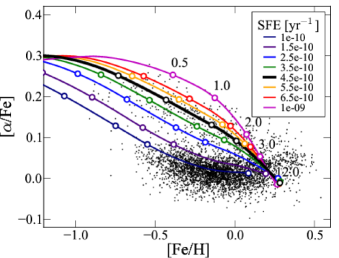
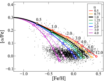
Figure 15.— Tracks in [$\alpha$/Fe] vs. [Fe/H] for GCE models with varying star formation efficiency (SFE, top) and outflow rate ($=\eta\times$SFR, middle), as marked in the legend. The labeled open circles indicate the abundance of each model at the given time in Gyr. The APOGEE–RC stars ($S/N$$>$150) are shown as filled black points. The heavy black curve indicates the fiducial model that best fits the observed high-$\alpha$ sequence. (Bottom) The star formation history of the GCE models normalized by the SFR of the fiducial model at t=2 Gyr.

5. Discussion

The empirical results presented in §4 provide stringent tests for chemo-dynamical models that can predict the distributions of iron and $\alpha$-element abundances as a function of Galactocentric radius and vertical position. In this section, we examine some of the broad conclusions that can be drawn from the data, supporting our interpretations with reference to simple one-zone models of Galactic chemical evolution (GCE). While these models do not attempt to provide a full account of the star formation and enrichment history of the Milky Way, they are a valuable tool for investigating parameter space to gain a qualitative grasp of the effects of the most important processes.

5.1. Galactic Chemical Evolution Model

The GCE model is one-zone with gas accretion and outflow. The inflow rate is an exponential in time with an $e$-folding time scale of 14 Gyr. The outflow rate is parametrized as $\eta\times$SFR, where $\eta$ is the outflow mass-loading parameter and $\eta=1.0$ for the fiducial model. We adopt the yields of Chieffi & Limongi (2004) and Limongi & Chieffi (2006) for SNII, the W70 model of Iwamoto et al. (1999) for SNIa, and Karakas (2010) for AGB stars. We assume a Kroupa (2001) initial mass function (IMF) from 0.1–100 M_⊙. The SNIa delay-time distribution is an exponential in time with an $e$-folding time scale of 1.5 Gyr and a minimum delay time of 150 Myr. The star formation rate is SFE$\times$M_gas, and we set the star formation efficiency (SFE) to be 4.5$\times$10^-10 yr^-1. The GCE model will be described in detail by B. Andrews et al. (2014, in preparation), who explore the impact of varying many different model inputs. For the purposes of this paper, the model [$\alpha$/Fe] is the average of [O/Fe], [Mg/Fe] and [Si/Fe], which are the dominant $\alpha$ elements in the APOGEE wavelength range. This fiducial model is compared to the APOGEE-RC data in Figure 14.

5.2. The High-$\alpha$ Sequence

An unexpected feature of the APOGEE–RC $\alpha$-element abundance distributions is the uniformity of the high-$\alpha$ sequence across the Galaxy. Figure 15 shows the dependence of GCE model tracks in the [$\alpha$/Fe] vs. [Fe/H] plane on the star formation efficiency (top) and outflow rate (middle), the two parameters that have the largest impact on the location of the high-$\alpha$ sequence. SFE determines the metallicity of the knee in [$\alpha$/Fe] vs. [Fe/H] (Pagel, 1997), and this in turn sets the location of the high-$\alpha$ sequence below about solar metallicity. When the SFE is high, core collapse SNe can enrich the ISM to higher [Fe/H] before Type Ia SNe become important and drive [$\alpha$/Fe] toward solar values. However, changing the SFE has minimal impact on the endpoint of the GCE track, a location in [$\alpha$/Fe] vs. [Fe/H] that we refer to as the model’s “equilibrium” abundance, because the evolution becomes very slow at late times. This equilibrium abundance is sensitive to the outflow rate, since with high $\eta$ the population cannot evolve to high [Fe/H], because it is losing metals too quickly. Fitting the observed location of the high-$\alpha$ sequence thus imposes tight constraints on both SFE and $\eta$, with the former constrained mainly by the locus below solar [Fe/H], and the latter by the locus above solar [Fe/H].

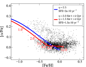
Figure 16.— Two GCE models intended to reproduce the low-$\alpha$ sequence in the [$\alpha$/Fe] vs. [Fe/H] plane. The blue line shows a model with an outflow rate of 2.5$\times$SFR and SFE=2$\times$10^-10 yr^-1, which reaches the density peak of the low-$\alpha$ sequence. The red line shows a model with a time-varying outflow rate ($\eta=3$ for $t<4$ Gyr and $\eta=1.5$ for $t>4$ Gyr) that runs through the whole low-$\alpha$ sequence. The labeled open circles indicate the abundance of each model at the given time in Gyr. The APOGEE–RC stars are shown as filled black points.

The constancy of the high-$\alpha$ sequence in the APOGEE–RC data implies surprising uniformity in the enrichment history of stars that now occupy a wide range of $R$ and $|Z|$. It is evident from Figure 15 that plausible model variations can shift the sequence by amounts much larger than allowed by the observations. If we treat SFE as the sole adjustable parameter, and fit the sequence in the nine zones of Figure 11, we find that the allowed variations are only $\sim 15\%$. There is some tradeoff between SFE and $\eta$, and other model inputs to a lesser degree, so more generally this constancy of location implies a surprising degree of uniformity in some combination of GCE parameters, with SFE being the most important one.

The implication of a similar SFE for the high-$\alpha$ stars across the Galaxy appears counter-intuitive because stars in the inner Galaxy should have formed more rapidly than in the outer Galaxy, due to higher gas densities. This in turn would shift the high-$\alpha$ sequence towards higher [Fe/H] at small radii. The SFE for the model that best reproduces the high-$\alpha$ sequence ($\sim 4.5\times 10^{-10}\,{\rm yr}^{-1}$) is remarkably similar to (within the SFE uncertainties) the nearly constant value ($\sim$5.25$\pm$2.5$\times$10^-10 yr^-1; across a diverse range of local environments) found by Leroy et al. (2008) for regions of nearby spiral galaxies (mostly in the inner parts) dominated by molecular gas (i.e., H₂). This suggests that the uniformity of the SFE in the early MW could be a product of an ISM dominated by molecular gas throughout the young, relatively compact disk. High molecular gas fractions of $\sim$40% are observed in star forming galaxies at z$\sim$2 (Tacconi et al., 2013), during the era when the MW thick disks are believed to have formed. Alternatively, the present distributions could partly be explained if high-$\alpha$ stars formed predominantly in a narrow, easily-mixed radial annulus in the inner Galaxy and subsequently migrated to larger radii, creating the more homogeneous chemical distribution observed today. It is beyond the scope of this paper to distinguish between these scenarios. However, observations of disk galaxies at high redshift reveal kinematically hot, turbulent systems that could contribute to more uniform star formation conditions across a range of radii (Section 5.5). Therefore, we find it somewhat more likely that the constancy of the high-$\alpha$ sequence was imprinted at birth, on a stellar population formed in a well-mixed, turbulent, and molecular-dominated ISM with a gas consumption timescale (SFE^-1) of $\sim 2$ Gyr.

5.3. Low-$\alpha$ Sequence

Another striking feature of the APOGEE results is the metallicity at which the high-$\alpha$ sequence merges with the low-$\alpha$ sequence, roughly [Fe/H]$\approx$+0.2 dex at all locations. In the inner Galaxy this value is close to the peak of the metallicity distribution function (MDF) of the low-$\alpha$ population, so it is possible to explain the low-$\alpha$ stars as the endpoint of the chemical evolution sequence that produced the high-$\alpha$ population. However, at the solar radius and in the outer Galaxy, the merging point of the two $\alpha$ sequences is at a significantly higher metallicity than the peak of the low-$\alpha$ MDF, by $\sim$0.2–0.3 dex. This offset makes it difficult (perhaps impossible) to explain the high-$\alpha$ and low-$\alpha$ stars as the outcome of a single chemical enrichment history, indicating the presence of at least two distinct populations. While this discrepancy has been seen before in the solar neighborhood (e.g., Bensby et al., 2011a; Adibekyan et al., 2013) the APOGEE RC sample presents the best-populated, most-accurate distributions yet and the first time this has been plainly seen in the outer Galaxy.

We now describe two different scenarios that could explain the observed chemical abundances patterns: (1) SFE–transition, and (2) superposition of multiple populations.

5.3.1 SFE Transition

Figure 16 illustrates two GCE models with parameters chosen to approximately reproduce the observed locus of the low-$\alpha$ stars with a single chemical evolutionary sequence. The blue line shows a model with a low SFE (2$\times$10^-10 yr^-1) and high outflow rate (2.5$\times$SFR) relative to the fiducial model that matches the high-$\alpha$ sequence. The low SFE shifts the knee of the model sequence to low [Fe/H], and the high value of $\eta$ shifts the late-time equilibrium abundance to solar [Fe/H]. The model does not produce stars with super-solar [Fe/H]. The red line shows an alternative model with still lower SFE and an outflow rate that changes from $\eta=3$ for $t<4$ Gyr to $\eta=1.5$ for $t>4$ Gyr. In this case, the low SFE and high initial $\eta$ drive the model quickly to the low metallicity end of the low-$\alpha$ locus, but the transition to low $\eta$ allows the model to retain more of the metals that it produces, and thus evolve to higher [Fe/H] at low [$\alpha$/Fe]. While a decrease in outflow efficiency at late times is physically plausible, as a result of decreased star formation rate and a thinner, more settled gas disk, we note that the parameters of this simulation have been quite finely tuned to match the location of the observed low-$\alpha$ locus. Small changes in the outflow mass-loading parameters or the timing of the switch from high to low outflow rate significantly alter the location of the track in [$\alpha$/Fe]–[Fe/H].

The GCE models can reproduce the observed chemical abundances patterns of the high-$\alpha$ sequence (high SFEH; Figure 14) and the low-$\alpha$ sequence (low SFE; Figure 16). However, attempts to explain both $\alpha$ groups with a single chemical evolution scenario require some special circumstances. Once the high-$\alpha$ stars reach low [$\alpha$/Fe] abundance ratios (after $\sim$3–4 Gyr in our GCE model consistent with the results of Snaith et al., 2014), their metallicites are higher than the majority of the younger low-[$\alpha$/Fe] stars (according to the ages of Haywood et al. 2013). Figure 10 of Haywood et al. (2013) demonstrates the difference in metallicity of $\sim$9–10 Gyr old stars between the high and low-$\alpha$ groups is $\sim$0.5 dex. To explain the evolution of the low-$\alpha$ stars from the gas left over from the formation of the high-$\alpha$ stars (minus the outflow), the gas would have to be depleted in metals without increasing the overall [$\alpha$/Fe] ratio. This condition can be accomplished by accretion of large amounts of pristine gas. However, if too much gas is accreted too quickly the star formation rate will rapidly increase and produce many SNII, further increasing the $\alpha$-element abundance ratios to high values. For example, to decrease the metallicity from [Fe/H]=$+$0.2 (where the high-$\alpha$ sequence reaches solar-$\alpha$) to [Fe/H]=$-$0.5 (the metal-poor end of the low-$\alpha$ sequence in the outer Galaxy) requires increasing the gas mass by $\sim$5 times without adding any metals (i.e., accretion of pristine gas). From the Kennicutt-Schmidt star formation law (Kennicutt 1989; $\Sigma_{\rm SFR}$ $\propto$ $\Sigma_{\rm gas}^{\rm n}$), this result implies an increase in the SFR of $\sim$9.5 to 25 with an exponent of n=1.4 and n=2, respectively. This enormous rise of the SFR, essentially a “starburst”, would cause a significant amplification in SNII and high $\alpha$-element production. In addition, the large star formation rate would overpredict the observed number of metal-poor stars. Therefore, the pristine gas has to be accreted on long timescales (e.g., Chiappini et al., 1997).

If the low- and high-$\alpha$ groups are interpreted as two evolutionary sequences (as presented above), then they have low and high SFE, respectively, and were formed in quite different physical environments. If the stars that we currently detect in the outer Galaxy all formed there, the existence of the two $\alpha$-element sequences could represent a dramatic shift in the SFE of the outer Galaxy $\sim$9 Gyr ago. In addition to the nearly constant SFE for molecular-dominated ISM, Leroy et al. (2008) found that regions with the ISM dominated by neutral hydrogen gas (H I) have SFE that decreases with radius. Since the outer portions of the MW are now dominated by atomic gas (e.g., Scoville & Sanders, 1987; Kulkarni & Heiles, 1987), we should expect the current SFE to decrease with radius and be low in the outer Galaxy consistent with the observed low SFE low-$\alpha$ sequence. One possible scenario is that early on the entire MW gaseous disk was dominated by molecular gas, producing a nearly uniform SFE and the high-$\alpha$ sequence of stars that we detect. After $\sim$4 Gyr, the ISM in the outer Galaxy transitioned from molecular-dominated gas (high SFE) to atomic-dominated gas (lower SFE decreasing with radius), reducing its SFE substantially (by $\sim$1/3), while the SFE in the inner Galaxy remained high. This scenario would produce a single high SFE sequence in the inner Galaxy, but a double SFE sequence in the outer Galaxy. The transition must have proceeded fairly rapidly to produce the observed $\alpha$-element bimodality. The decrease in SFE in the outer Galaxy must have been accompanied by a decrease in ISM metallicity to explain the metal-poor low-$\alpha$ stars, thus requiring an infall of pristine gas. The decrease of SFE combined with a long infall timescale of the pristine gas would help keep the $\alpha$-abundance ratios low during this active transition period.

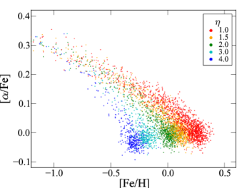
Figure 17.— A scenario in which the low-$\alpha$ locus results from the superposition of populations with different enrichment histories. The different colored points indicate the stellar populations formed by five different GCE models with outflow rates as marked in the legend. The models shown by the red, orange, and green points have an inflow $e$-folding timescale of 14 Gyr, and the blue and cyan models have a constant SFR. The red points are from the fiducial high-$\alpha$ model of Figure 15. Gaussian noise of $\sigma=0.05$ in [Fe/H] and $\sigma=0.02$ in [$\alpha$/Fe] was added to the tracks to show overlapping data points and for ease of comparison with the data.

While the SFE-transition scenario appears to be a qualitatively viable interpretation of our results, it also predicts that there should be a fairly rapid transition between the two SFE values and $\alpha$-element sequences that is not entirely consistent with what is observed. The Haywood et al. (2013) data (see their Figure 10) indicate a significant overlap in age between the metal-rich end of the high-$\alpha$ sequence and the metal-poor end of the low-$\alpha$ sequence. While the overlap could partly be explained by uncertainties in the derived ages, it nevertheless complicates the SFE-transition scenario.

A close inspection of the GCE model for the low-$\alpha$ stars in Figure 16 indicates that, while this track fits the observed low-$\alpha$ sequence fairly well, there is a dearth of observed low-metallicity and intermediate-$\alpha$ stars in the early part of the track. These objects are the early “progenitor” stars that would have been formed in an ISM dominated by SNII and high-$\alpha$ abundances and that would eventually produce the SNIa to lower the $\alpha$-element abundance. If the low-$\alpha$ sequence of stars formed in “isolation”, these progenitor stars should exist, and we should be able to detect them. These types of stars have recently been found in the Fornax dwarf spheroidal Galaxy (Hendricks et al., 2014a), in an environment with even lower SFR than the outer MW disk. Even though our RC sample is biased against metal-poor stars, we should detect stars down to [Fe/H]=$-$0.9, well-below the observed low-$\alpha$ cutoff of [Fe/H]$\sim$$-$0.5. Additionally, the lack of progenitor stars for the low-$\alpha$ sequence is evident in independent samples that probe to lower metallicities, such as Fuhrmann (2011, cutoff at [Fe/H]$\geq$$-$0.6), Adibekyan et al. (2013, cutoff at [Fe/H]$\geq$$-$0.7), and Bensby et al. (2014, cutoff at [Fe/H]$\geq$$-$0.7), which suggests that the paucity of these stars is real.

The lack of progenitor stars of the low-$\alpha$ sequence suggests that the low-$\alpha$ sequence began its evolution in a low $\alpha$-element abundance ISM. This scenario could be produced by the stars in the high-$\alpha$ sequence which formed first polluting the ISM with low-$\alpha$ metals. This is a natural consequence in the SFE-transition scenario, since the low-SFE low-$\alpha$ sequence does not start its evolution with pristine gas, but with the gas chemically enriched by the high-SFE high-$\alpha$ sequence over $\sim$4 Gyr to low-$\alpha$ abundances. But, even if the high-$\alpha$ stars formed somewhere else (i.e., in the inner Galaxy), and then moved to their current locations, they could continuously pollute (pristine accreted) gas in the outer Galaxy at a low level, causing any new stars formed there to be pre-enriched to a low-$\alpha$ level. This process essentially causes the low-$\alpha$ chemical evolutionary sequence to start abruptly at low/intermediate-$\alpha$ and intermediate metallicity ([Fe/H]$\sim$$-$0.7) which is unexpected from a simple chemical evolutionary analysis. Additionally, any chemically pristine accreted gas in the outer Galaxy could have been polluted by low-$\alpha$ outflow from the inner Galaxy. The Haywood et al. (2013) ages indicate that the high-$\alpha$ sequence started $\sim$13 Gyr ago, while the low-$\alpha$ sequence started $\sim$10 Gyr ago. By $\sim$10 Gyr ago the high-$\alpha$ sequence had reached a low enough $\alpha$-element abundance to match those observed for the oldest low-$\alpha$ stars, albeit at different metallicities (upper panel of Figure 7 of Haywood et al. 2013). Not much ($\sim$1/4) intermediate-$\alpha$ metal-rich gas is needed to pollute the pristine gas in the outer Galaxy to produce the observed metallicity and $\alpha$-element abundance for the oldest stars in the low-$\alpha$ sequence. This explanation requires continuous injection of enriched gas into the outer Galaxy until the onset of in situ SNIa’s, as well as a fine-tuning of the start of star formation in the outer Galaxy with the chemical evolution of the inner Galaxy.

5.3.2 Superposition of Multiple Populations

The tendency of the models to settle at an equilibrium abundance suggests an alternative scenario, illustrated in Figure 17, in which the low-$\alpha$ locus is not itself an evolutionary sequence but a superposition of populations that have different star formation and enrichment histories. Here we have drawn stars randomly from the outputs of five models with different outflow rates, one of them (red points) having the same parameters as the fiducial model used to fit the high-$\alpha$ sequence, and the other four with higher $\eta$ values that shift their endpoints to lower [Fe/H]. The three rightmost models (red, orange, and green points) have inflow with a 14 Gyr $e$-folding timescale, while the other two have a constant (instead of declining) SFR, to increase their equilibrium [$\alpha$/Fe]. All of the other model parameters are the same as those of the fiducial high-$\alpha$ model. The final stellar mass of the low-$\eta$ model is three times that of the highest-$\eta$ models, because of the differing accretion history and greater retention of ISM gas. We added Gaussian noise ($\sigma=0.05$ dex for [Fe/H] and $\sigma=0.02$ dex for [$\alpha$/Fe]) to help visualize the relative numbers of stars with similar abundances, and compare to the observed locus. Each model produces the great majority of its stars close to its endpoint, because early evolution is much more rapid, and the multiple endpoints merge to form a locus of stars with a range of [Fe/H] but roughly solar [$\alpha$/Fe]. This picture roughly resembles the scenario put forward by Schönrich & Binney (2009a), in which stars form with different enrichment histories as a function of galactocentric radius, and the key mechanism for producing a superposition of populations is radial migration of stars away from their birth radii.

An appealing feature of the superposition scenario is its ability to explain the shift in the [Fe/H] centroid of the low-$\alpha$ locus with radius. This picture requires a low $\eta$ in the inner Galaxy, producing the high-$\alpha$ sequence and low-$\alpha$, super-solar [Fe/H] stars at its endpoint, and higher $\eta$ at larger Galactocentric radius to produce tracks with lower equilibrium [Fe/H]. More efficient outflows could arise in the outer Galaxy because of a weaker vertical potential and a lower density of ISM gas to damp energy injection from supernovae. Radial gas flows within the disk can also have a similar effect to radially increasing $\eta$, by advecting metals produced in the outer disk inward to smaller radii. While the relative weight of different populations shifts with radius in this scenario, the APOGEE data show that the high-$\alpha$ sequence is present at all radii, and is either the relic of an early epoch of star formation or a population formed in one region that has spread through the Galaxy over time.

An encouraging feature of Figure 17 is that it retains bimodality of the [$\alpha$/Fe] distribution at all metallicities, with a broader gap at low [Fe/H]. The younger stars of the high-$\eta$ populations have intermediate values of [$\alpha$/Fe], but the frequency of these intermediate stars appears at least qualitatively consistent with the APOGEE data. The high-$\alpha$ sequence follows the track of the low-$\eta$ model, in part because it produces the most stars at early times, but also because the tracks of all five models merge at low [Fe/H], producing a clear ridge line in the diagram. There are quantitative discrepancies between the simulated and observed populations, and in any case a full model must do more than superpose the results of independent calculations with tuned parameter choices; it must present a full inflow, star formation, and outflow history as a function of Galactic position, and specify whatever mechanisms led to mixing of stellar populations. The comparisons in Figures 15, 16, and 17 indicate some of the characteristics that will be required in a successful model, and they show that the empirical regularities found in the APOGEE-RC data imply some significant complexities in the enrichment history of the Milky Way.

5.4. Comparison to Density Measurements

This paper has focused on the shape of the high- and low-$\alpha$ sequences and what they imply for the chemical history of the MW. The relative fraction of stars along each sequence and its spatial dependence holds important additional clues about how the two sequences formed and were shaped by evolution. From the radial dependence of the relative fraction of high- and low-$\alpha$ stars we conclude that the high-$\alpha$ sequence is primarily associated with the inner Galaxy, while the low-$\alpha$ stars are most prominent in the outer Galaxy. This interpretation is in qualitative agreement with the measurement of the large radial scale length of low-$\alpha$ populations compared to that of high-$\alpha$ populations from SEGUE (Bovy et al., 2012b). Figure 11 also suggests that the lowest $[\mathrm{Fe/H}]$, high-$\alpha$ stars are typically found at larger $Z$ than the higher $[\mathrm{Fe/H}]$, high-$\alpha$ stars. This figure shows that this is the case even at fixed [$\alpha$/Fe]. This result is also in qualitative agreement with the vertical-scale-height measurements of Bovy et al. (2012b) and the vertical-metallicity-gradient measurements of Schlesinger et al. (2014) and Boeche et al. (2014). In future work, we intend to use the APOGEE data directly to measure the spatial and kinematic distributions of stars along the high- and low-$\alpha$ sequence. Combined with age dating of the $\alpha$-element sequences, these measurements will allow us to distinguish between different scenarios for the origin of the thick disk components in the MW.

5.5. Simulations and the Extragalactic Context

The uniform enrichment history of the high-$\alpha$ sequence is predicted by a simple one-zone model. The physical conditions necessary for one-zone evolution naturally occur in a thin radial annulus of the young MW disk ($\Delta r<\sim 1$ kpc), where differential rotation and small-scale turbulence can adequately homogenize the gas-phase metallicity as assumed in many GCE frameworks (e.g., Clayton, 1986; Matteucci & Francois, 1989). If born in a small range of formation radii, the high-$\alpha$ sequence stars must subsequently migrate throughout the Galaxy to match their currently observed configuration. Alternatively, large-scale turbulence could mix star-forming gas over longer distances, widening the formation annulus of the high-$\alpha$ sequence, and lessening the required degree of radial mixing. While neither scenario can be ruled out, a well-mixed, globally turbulent young Galaxy is corroborated by evidence from high-redshift observations. Rotationally-dominated disks observed at $z\sim 2$ exhibit large random motions, and are geometrically thick relative to local galaxies in both ionized (e.g., Epinat et al., 2012; Genzel et al., 2008, ; and references therein) and molecular (e.g., Swinbank et al., 2012; Tacconi et al., 2013) gas studies. Edge-on UV observations reveal that stellar disks have similar scale heights to the ionized gas in these systems (e.g., Elmegreen & Elmegreen, 2006). If the inferred early dynamical history of the MW is typical of disk galaxies, our findings offer an important constraint on galaxy formation models that predict stellar kinematics over a range of redshift. Numerical simulations in which the early disk forms via a gas-rich merger (Brook et al., 2004), clumpy star-formation (Bournaud et al., 2009), or in situ star formation from a turbulent star-forming gas reservoir (e.g., Bird et al., 2013), all qualitatively match the relatively large velocity dispersions and degree of mixing required by the constant high-$\alpha$ sequence.

The likely one-zone origin of the high-$\alpha$ sequence also suggests that the MW’s radial chemical gradient was nearly flat in the past, and has steepened over time to its current value. There is conflicting evidence as to the slope of chemical gradients in high redshift galaxies (e.g., Yuan et al., 2013). Some studies of $z>1$ galaxies report relatively steep chemical gradients (e.g., Jones et al., 2010; Yuan et al., 2011), while larger samples suggest that gradients were more shallow than those found in local spirals (Queyrel et al., 2012; Swinbank et al., 2012). The temporal evolution of the radial chemical gradient can constrain the uncertain degree to which energetic feedback mechanisms couple to the ISM and redistribute metals in simulations of disk galaxy formation (Gibson et al., 2013). Conservative feedback prescriptions predict initially steep gradients that flatten over time, while models with ’enhanced’ feedback physics create flatter gradients at early times that subsequently steepen (Pilkington et al., 2012; Gibson et al., 2013). Relatively strong feedback is already required to form disk galaxies with realistic bulge-to-disk ratios (e.g., Guedes et al., 2011) and to reproduce the stellar mass - halo mass relationship (Munshi et al., 2013; Stinson et al., 2013) found using an abundance-matching approach (e.g., Moster et al., 2013). Our results are broadly consistent with these ’enhanced’ feedback models. The constant high-$\alpha$ sequence suggests that the chemical radial gradient of the MW has become increasingly negative with time.

The persistent valley between the low- and high-$\alpha$ sequences is not readily reproduced by numerical experiments of MW-like galaxies. The chemical composition distributions of simulated stellar populations generically show either a single or multiple sequence progression from low-metallicity, high-$\alpha$ to high-metallicity, low-$\alpha$ regions in the [O/Fe], [Fe/H] plane (e.g., Brook et al., 2012; Minchev et al., 2013; Stinson et al., 2013); others report relatively flat variation of [O/Fe] with [Fe/H] (e.g., Marinacci et al., 2014). While some simulations produce low-metallicity, low-$\alpha$ stars (e.g., Roškar et al., 2013), they fail to reproduce the observed intermediate-$\alpha$ valley. A variety of modeling techniques and numerical codes are unable to recreate the two-dimensional chemical abundance structure observed in the MW. Therefore, potential origins of the valley are likely to originate in uncertainties inherent to all simulations, i.e., the star-formation prescription, feedback implementations governing mass outflow, and the accretion histories of both satellite galaxies and gas. Both the spatially-independent high-$\alpha$ sequence and valley are robust structures in the [$\alpha$/Fe], [Fe/H] plane that offer a promising new avenue of direct comparison with galaxy formation models.

6. Conclusions

We use the APOGEE red clump sample of $\sim$10,000 stars to map the $\alpha$-abundance patterns across a large volume of the Milky Way disk (5$<$R$<$11 kpc and 0$<$$|$Z$|$$<$2 kpc). Selection effects for our sample due to the APOGEE targeting strategy and volume probed are characterized and found not to adversely affect the abundance patterns. Our main results and conclusions are as follows:

1. A bimodality in [$\alpha$/Fe] is detected at low metallicity ($-$0.9$<$[Fe/H]$<$$-$0.2) throughout the Galaxy. This result is not affected by the APOGEE targeting and field selection functions. The low- and high-$\alpha$ abundance sequences merge at high metallicity ([Fe/H]$\approx$$+$0.2).

2. The shape of the high-$\alpha$ sequence in the [$\alpha$/Fe] vs. [Fe/H] diagram is quite constant and varies little across the Galaxy. The small spatial variations show a slight negative radial gradient that increases towards the midplane, but the overall variations are only $\sim$10%. The fact that the high-$\alpha$ sequence in the Galactic bulge is similar to the local one (Bensby et al., 2011b), in combination with our results implies that the high-$\alpha$ sequence remains nearly constant all the way to the Galactic center.

3. Using simple galactic chemical evolution models we derive an average star formation efficiency (SFE) in the high-$\alpha$ sequence of $\sim$4.5$\times$10^-10 yr^-1 which is quite close to the nearly-constant SFE value for regions of nearby spiral galaxies dominated by molecular gas. The homogeneity of the high-$\alpha$ sequence implies that these stars share a similar star formation history and were formed in a well-mixed, turbulent, and molecular-dominated ISM with a gas consumption timescale (SFE^-1) of $\sim 2$ Gyr.

4. The behavior of the high- and low-$\alpha$ sequences as a function of Galactocentric radius shows that the high-$\alpha$ sequence is more prominent in the inner Galaxy ($R$$\lesssim$$R_{0}$), while the low-$\alpha$ sequence is more prominent in the outer Galaxy.

5. While the stars in the inner Galaxy can be explained by a single chemical evolutionary track, this cannot be done in the outer Galaxy, indicating the presence of at least two distinct populations.

A possible expanation for the homogeneity in the shape of the high-$\alpha$ sequence throughout the Galaxy is that the ISM of the early Milky Way was dominated by molecular gas, which has been shown to have a nearly constant SFE across diverse physical environments and similar to the value that we measure. We also discuss two possible scenarios to explain the low-$\alpha$ sequence (especially in the outer Galaxy): (1) The gas transitions from high SFE to low SFE coupled with accretion of pristine gas $\sim$8 Gyr ago. While this scenario is qualitatively consistent with many of our results, it is not clear if it agrees in detail with the abundances and ages of Haywood et al. (2013) and requires further investigation. (2) The low-$\alpha$ sequence is composed of a superposition of multiple populations covering a range of outflow rates and final [Fe/H] on the low-$\alpha$ end. Mixing of populations formed at different radii could explain the radial metallicity gradient and the chemical abundance patters in the outer Galaxy.

References

- Abadi et al. (2003) Abadi, M. G., Navarro, J. F., Steinmetz, M., & Eke, V. R. 2003, ApJ, 597, 21
- Adibekyan et al. (2011) Adibekyan, V. Z., Santos, N. C., Sousa, S. G., & Israelian, G. 2011, A&A, 535, L11
- Adibekyan et al. (2012) Adibekyan, V. Z., Sousa, S. G., Santos, N. C., et al. 2012, A&A, 545, A32
- Adibekyan et al. (2013) Adibekyan, V. Z., Figueira, P., Santos, N. C., et al. 2013, A&A, 554, A44
- Ahn et al. (2014) Ahn, C. P., Alexandroff, R., Allende Prieto, C., et al. 2014, ApJS, 211, 17
- Allende Prieto et al. (2006) Allende Prieto, C., Beers, T. C., Wilhelm, R., et al. 2006, ApJ, 636, 804
- Allende-Prieto et al. (2014) Allende-Prieto, C., Koesterke, L., Shetrone, M. D., et al. 2014, American Astronomical Society Meeting Abstracts #223, 223, #440.05
- Anders et al. (2014) Anders, F., Chiappini, C., Santiago, B. X., et al. 2014, A&A, 564, A115
- Audouze & Tinsley (1976) Audouze, J. Tinsley, B. M. 1976, ARA&A, 14, 43
- Barklem et al. (2012) Barklem, P. S., Belyaev, A. K., Spielfiedel, A., et al. 2012, A&A, 541, A80
- Barklem et al. (2000) Barklem, P.S., Piskunov, N., & O’Mara, B.J. 2000, A&A, 355, L5
- Belyaev & Barklem (2003) Belyaev, A. K. & Barklem, P. S. 2003, Phys. Rev., A 68, 062703
- Belyaev et al. (2010) Belyaev, A. K., Barklem, P. S., Dickinson, A. S., & Gadéa, F. X. 2010, Phys. Rev. A, 81, 032706
- Bensby et al. (2005) Bensby, T., Feltzing, S., Lundström, I., & Ilyin, I. 2005, A&A, 433, 185
- Bensby et al. (2007) Bensby, T., Zenn, A.R., Oey, M.S. ,Feltzing, S., 2007, ApJ, 663, L13
- Bensby et al. (2011a) Bensby, T., Alves-Brito, A., Oey, M. S., Yong, D., & Meléndez, J. 2011, ApJ, 735, L46
- Bensby et al. (2011b) Bensby, T., Yee, J. C., Feltzing, S., et al. 2011b, A&A, 549, A147
- Bensby et al. (2014) Bensby, T., Feltzing, S., & Oey, M. S. 2014, A&A, 562, A71
- Bergemann et al. (2014) Bergemann, M., Ruchti, G. R., Serenelli, A., et al. 2014, A&A, 565, A89
- Bienaymé et al. (1987) Bienaymé, O., Robin, A. C., & Crézé, M. 1987, A&A, 180, 94
- Binney et al. (1991) Binney, J., Gerhard, O. E., Stark, A. A., Bally, J., & Uchida, K. I. 1991, MNRAS, 252, 210
- Bird et al. (2013) Bird, J. C., Kazantzidis, S., Weinberg, D. H., et al. 2013, ApJ, 773, 43
- Boeche et al. (2014) Boeche, C., Siebert, A., Piffl, T., et al. 2014, A&A, 568, A71
- Bournaud et al. (2009) Bournaud, F., Elmegreen, B. G., & Martig, M. 2009, ApJ, 707, L1
- Bovy et al. (2012a) Bovy, J., Rix, H.-W., & Hogg, D. W. 2012a, ApJ, 751, 131
- Bovy et al. (2012b) Bovy, J., Rix, H.-W., Liu, C., et al. 2012b, ApJ, 753, 148
- Bovy et al. (2012c) Bovy, J., Rix, H.-W., Hogg, D. W., et al. 2012c, ApJ, 755, 115
- Bovy et al. (2014) Bovy, J., Nidever, D. L., Rix, H.-W., et al. 2014, ApJ, 790, 127
- Bressan et al. (2012) Bressan, A., Marigo, P., Girardi, L., et al. 2012, MNRAS, 427, 127
- Brook et al. (2004) Brook, C. B., Kawata, D., Gibson, B. K., & Freeman, K. C. 2004, ApJ, 612, 894
- Brook et al. (2012) Brook, C. B., Stinson, G. S., Gibson, B. K., et al. 2012, MNRAS, 426, 690
- Chen et al. (2003) Chen, L., Hou, J. L., & Wang, J. J. 2003, AJ, 125, 1397
- Cheng et al. (2012) Cheng, J. Y., Rockosi, C. M., Morrison, H. L., et al. 2012a, ApJ, 746, 149
- Cheng et al. (2012) Cheng, J., Rockosi, C. M., Morrison, H. L., et al. 2012b, ApJ, 752, 51
- Chiappini et al. (1997) Chiappini, C., Matteucci, F., & Gratton, R. 1997, ApJ, 477, 765
- Chiappini (2009) Chiappini, C. 2009, IAU Symposium, 254, 191
- Chieffi & Limongi (2004) Chieffi, A., & Limongi, M. 2004, ApJ, 608, 405
- Churchwell et al. (2009) Churchwell, E., Babler, B. L., Meade, M. R., et al. 2009, PASP, 121, 213
- Clayton (1986) Clayton, D. D. 1986, PASP, 98, 968
- de Bruijne (2012) de Bruijne, J. H. J. 2012, Ap&SS, 681
- Eisenstein et al. (2011) Eisenstein, D. J., Weinberg, D. H., Agol, E., et al. 2011, AJ, 142, 72
- Elmegreen & Elmegreen (2006) Elmegreen, B. G., & Elmegreen, D. M. 2006, ApJ, 650, 644
- Epinat et al. (2012) Epinat, B., Tasca, L., Amram, P., et al. 2012, A&A, 539, A92
- Förster Schreiber et al. (2011) Förster Schreiber, N. M., Shapley, A. E., Erb, D. K., et al. 2011, ApJ, 731, 65
- Fuhrmann (1998) Fuhrmann, K. 1998, A&A, 338, 161
- Fuhrmann (2011) Fuhrmann, K. 2011, MNRAS, 414, 2893
- García Pérez et al. (2013) García Pérez, A. E., Cunha, K., Shetrone, M., et al. 2013, ApJ, 767, L9
- Genzel et al. (2008) Genzel, R., Burkert, A., Bouché, N., et al. 2008, ApJ, 687, 59
- Gibson et al. (2013) Gibson, B. K., Pilkington, K., Brook, C. B., Stinson, G. S., & Bailin, J. 2013, A&A, 554, A47
- Gilmore & Reid (1983) Gilmore, G., & Reid, N. 1983, MNRAS, 202, 1025
- Gilmore (1984) Gilmore, G. 1984, MNRAS, 207, 223
- Girardi et al. (2002) Girardi, L., Bertelli, G., Bressan, A., Chiosi, C., Groenewegen, M. A. T., Marigo, P., Salasnich, B., & Weiss, A. 2002, A&A, 391, 195
- Girardi et al. (2012) Girardi, L., Barbieri, M., Groenewegen, M. A. T., et al. 2012, Red Giants as Probes of the Structure and Evolution of the Milky Way, 165
- Groenewegen (2008) Groenewegen, M. A. T. 2008, A&A, 488, 935
- Guedes et al. (2011) Guedes, J., Callegari, S., Madau, P., & Mayer, L. 2011, ApJ, 742, 76
- Gunn et al. (2006) Gunn, J. E., Siegmund, W. A., Mannery, E. J., et al. 2006, AJ, 131, 2332
- Gustafsson et al. (2008) Gustafsson, B., Edvardsson, B., Eriksson, K., Jorgensen, U. G., Nordlund, A, & Plez, B. 2008, A&A, 486, 951
- Hammersley et al. (2000) Hammersley, P. L., Garzón, F., Mahoney, T. J., López-Corredoira, M., & Torres, M. A. P. 2000, MNRAS, 317, L45
- Hayden et al. (2014) Hayden, M. R., Holtzman, J. A., Bovy, J., et al. 2014, AJ, 147, 116
- Haywood et al. (2013) Haywood, M., Di Matteo, P., Lehnert, M. D., Katz, D., & Gómez, A. 2013, A&A, 560, A109
- Hendricks et al. (2014a) Hendricks, B., Koch, A., Lanfranchi, G. A., et al. 2014a, ApJ, 785, 102
- Holmberg et al. (2007) Holmberg, J., Nordström, B., & Andersen, J. 2007, A&A, 475, 519
- Kennicutt (1989) Kennicutt, R. C., Jr. 1989, ApJ, 344, 685
- Iwamoto et al. (1999) Iwamoto, K., Brachwitz, F., Nomoto, K., et al. 1999, ApJS, 125, 439
- Jones et al. (2010) Jones, T., Ellis, R., Jullo, E., & Richard, J. 2010, ApJ, 725, L176
- Kazantzidis et al. (2008) Kazantzidis, S., Bullock, J. S., Zentner, A. R., Kravtsov, A. V., & Moustakas, L. A. 2008, ApJ, 688, 254
- Karakas (2010) Karakas, A. I. 2010, MNRAS, 403, 1413
- Kroupa (2001) Kroupa, P. 2001, MNRAS, 322, 231
- Kulkarni & Heiles (1987) Kulkarni, S. R., & Heiles, C. 1987, Interstellar Processes, 134, 87
- Larson (1976) Larson, R. B. 1976, MNRAS, 176, 31
- Lee et al. (2011) Lee, Y. S., Beers, T. C., An, D., et al. 2011, ApJ, 738, 187
- Leroy et al. (2008) Leroy, A. K., Walter, F., Brinks, E., et al. 2008, AJ, 136, 2782
- Limongi & Chieffi (2006) Limongi, M., & Chieffi, A. 2006, ApJ, 647, 483
- Majewski (1993) Majewski, S. R. 1993, ARA&A, 31, 575
- Majewski et al. (2000) Majewski, S. R., Ostheimer, J. C., Kunkel, W. E., & Patterson, R. J. 2000, AJ, 120, 2550
- Majewski et al. (2010) Majewski, S. R., Wilson, J. C., Hearty, F., Schiavon, R. R., & Skrutskie, M. F. 2010, IAU Symposium, 265, 480
- Majewski et al. (2011) Majewski, S. R., Zasowski, G., & Nidever, D. L. 2011, ApJ, 739, 25
- Maoz et al. (2011) Maoz, D., Mannucci, F., Li, W., et al. 2011, MNRAS, 412, 1508
- Marinacci et al. (2014) Marinacci, F., Pakmor, R., Springel, V., & Simpson, C. M. 2014, MNRAS, 442, 3745
- Matteucci & Francois (1989) Matteucci, F., & Francois, P. 1989, MNRAS, 239, 885
- Mészáros et al. (2013) Mészáros, S., Holtzman, J., García Pérez, A. E., et al. 2013, AJ, 146, 133
- Minchev et al. (2012b) Minchev, I., Famaey, B., Quillen, A. C., et al. 2012b, A&A, 548, A127
- Minchev et al. (2013) Minchev, I., Chiappini, C., & Martig, M. 2013, A&A, 558, A9
- Moster et al. (2013) Moster, B. P., Naab, T., & White, S. D. M. 2013, MNRAS, 428, 3121
- Munshi et al. (2013) Munshi, F., Governato, F., Brooks, A. M., et al. 2013, ApJ, 766, 56
- Nidever et al. (2012) Nidever, D. L., Zasowski, G., Majewski, S. R., et al. 2012, ApJ, 755, L25
- Pagel (1997) Pagel, B. E. J. 1997, Nucleosynthesis and Chemical Evolution of Galaxies, (Cambridge, UK: Cambridge University Press)
- Pilkington et al. (2012) Pilkington, K., Few, C. G., Gibson, B. K., et al. 2012, A&A, 540, A56
- Plez (2012) Plez, B. 2012, Turbospectrum: Code for spectral synthesis, Astrophysics Source Code Library, record ascl:1205.004
- Prochaska et al. (2000) Prochaska, J. X., Naumov, S. O., Carney, B. W., McWilliam, A., & Wolfe, A. M. 2000, AJ, 120, 2513
- Queyrel et al. (2012) Queyrel, J., Contini, T., Kissler-Patig, M., et al. 2012, A&A, 539, A93
- Quinn et al. (1993) Quinn, P. J., Hernquist, L., & Fullagar, D. P. 1993, ApJ, 403, 74
- Ramírez et al. (2007) Ramírez, I., Allende Prieto, C., & Lambert, D. L. 2007, A&A, 465, 271
- Ramírez et al. (2013) Ramírez, I., Allende Prieto, C., & Lambert, D. L. 2013, ApJ, 764, 78
- Recio-Blanco et al. (2014) Recio-Blanco, A., de Laverny, P., Kordopatis, G., et al. 2014, A&A, 567, A5
- Reddy et al. (2006) Reddy, B. E., Lambert, D. L., & Allende Prieto, C. 2006, MNRAS, 367, 1329
- Rix & Bovy (2013) Rix, H.-W. & Bovy, J. 2013, A&A Rev., 21, 61
- Robin et al. (2003) Robin, A. C., Reylé, C., Derrière, S., & Picaud, S. 2003, A&A, 409, 523
- Robin et al. (2012) Robin, A. C., Marshall, D. J., Schultheis, M., & Reylé, C. 2012, A&A, 538, A106
- Roškar et al. (2013) Roškar, R., Debattista, V. P., & Loebman, S. R. 2013, MNRAS, 433, 976
- Schlesinger et al. (2012) Schlesinger, K. J., Johnson, J. A., Rockosi, C. M., et al. 2012, ApJ, 761, 160
- Schlesinger et al. (2014) Schlesinger, K. J., Johnson, J. A., Rockosi, C. M., et al. 2014, ApJ, 791, 112
- Schönrich & Binney (2009a) Schönrich, R., & Binney, J. 2009a, MNRAS, 396, 203
- Schönrich & Binney (2009b) Schönrich, R., & Binney, J. 2009b, MNRAS, 399, 1145
- Scoville & Sanders (1987) Scoville, N. Z., & Sanders, D. B. 1987, Interstellar Processes, 134, 21
- Sellwood & Binney (2002) Sellwood, J. A. & Binney, J.J. 2002, MNRAS, 336, 785
- Skrutskie et al. (2006) Skrutskie, M. F., Cutri, R. M., Stiening, R., et al. 2006, AJ, 131, 1163
- Smith et al. (2013) Smith, V. V., Cunha, K., Shetrone, M. D., et al. 2013, ApJ, 765, 16
- Snaith et al. (2014) Snaith, O. N., Haywood, M., Di Matteo, P., et al. 2014, ApJ, 781, L31
- Stinson et al. (2013) Stinson, G. S., Bovy, J., Rix, H.-W., et al. 2013, MNRAS, 436, 625
- Swinbank et al. (2012) Swinbank, A. M., Sobral, D., Smail, I., et al. 2012, MNRAS, 426, 935
- Tacconi et al. (2010) Tacconi, L. J., Genzel, R., Neri, R., et al. 2010, Nature, 463, 781
- Tacconi et al. (2013) Tacconi, L. J., Neri, R., Genzel, R., et al. 2013, ApJ, 768, 74
- van den Bergh (1962) van den Bergh, S. 1962, AJ, 67, 486
- Vera-Ciro et al. (2014b) Vera-Ciro, C., D’Onghia, E., Navarro, J., & Abadi, M. 2014b, ApJ, submitted (arXiv:1405.3317)
- Wilson et al. (2010) Wilson, J. C., Hearty, F., Skrutskie, M. F., et al. 2010, Proc. SPIE, 7735, 46
- Wilson et al. (2012) Wilson, J. C., Hearty, F., Skrutskie, M. F., et al. 2012, Proc. SPIE, 8446,
- Wright et al. (2010) Wright, E. L., Eisenhardt, P. R. M., Mainzer, A. K., et al. 2010, AJ, 140, 1868
- Yoachim & Dalcanton (2006) Yoachim, P., & Dalcanton, J. J. 2006, AJ, 131, 226
- Yoshii (1982) Yoshii, Y. 1982, PASJ, 34, 365
- Yuan et al. (2011) Yuan, T.-T., Kewley, L. J., Swinbank, A. M., Richard, J., & Livermore, R. C. 2011, ApJ, 732, L14
- Yuan et al. (2013) Yuan, T.-T., Kewley, L. J., & Rich, J. 2013, ApJ, 767, 106
- Zasowski et al. (2013) Zasowski, G., Johnson, J. A., Frinchaboy, P. M., et al. 2013, AJ, 146, 81