Classical Bianchi type I cosmology in K-essence theory

Abstract

We use one of the simplest forms of the K-essence theory and we apply it to the classical anisotropic Bianchi type I cosmological model, with a barotropic perfect fluid ($p=\gamma\rho$) modeling the usual matter content and with cosmological constant $\Lambda$, corresponding at case $\rm V(\phi)=2\Lambda$ in the K-essence lagrangian density. The classical solutions for any $\gamma\not=1$ and $\Lambda=0$ are found in closed form, using a time transformation. We also present the solution when $\Lambda\not=0$ including particular values in the barotropic parameter. We present the possible isotropization of the cosmological model Bianchi I using the ratio between the anisotropic parameters and the volume of the universe and show that this tend to a constant or to zero for different cases. Also we include a qualitative analysis of the analog of the Friedmann equation when it is written as an equation for the volume that is equivalent to the equation of motion of a particle under a potential and we conclude the same about the isotropization of this anisotropic models for the stiff and radiation eras of the universe, in the field $\phi$.

Keywords: K-essence theory; anisotropic model; classical solution;

I Introduction

In recent times, some attempts to unify the description of dark matter, dark energy and inflation, by means of a scalar field with non standard kinetic term have been conducted s-b ; armendariz ; bose ; jorge ; jorge1 . The K-essence theory is based on the idea of a dynamical attractor solution which causes it to act as a cosmological constant only at the onset of matter domination. Consequently, K-essence overtakes the matter density and induces cosmic acceleration at about the present epoch. Usually K-essence models are restricted to the lagrangian density of the form roland ; chiba ; bose ; arroja ; tejeiro

$$\rm S=\int d^{4}x\,\sqrt{-g}\,\left[f(\phi)\,{\cal G}(X)-V(\phi)\right],$$ (1)

where the canonical kinetic energy is given by $\rm{\cal G}(X)=X=-\frac{1}{2}\nabla_{\mu}\phi\nabla^{\mu}\phi$. K-essence was originally proposed as a model for inflation, and then as a model for dark energy, along with explorations of unifying dark energy and dark matter roland ; bilic ; bento . Another motivations to consider this type of lagrangian originates from string theory string . For more details for K-essence applied to dark energy you can see copeland and references therein.

In this framework, gravitational and matter variables have been reduced to a finite number of degrees of freedom. For homogenous cosmological models the metric depends only on time and gives a model with a finite dimensional configuration space, called minisuperspace. In this work, we use this formulation to obtain classical solutions to the anisotropic Bianchi type I cosmological model with a perfect fluid. This class of models were considered initially in this formalism by Chimento and Forte chimento . The first step is to write the theory for the Bianchi type I model in the usual manner, that is, we calculate the corresponding energy-momentum tensor to the scalar field and give the equivalent Lagrangian density. Next, by means of a Legendre transformation, we proceed to obtain the canonical Lagrangian ${\cal L}_{can}$, from which the classical Hamiltonian ${\cal H}$ can be found.

One of the simplest K-essence models, without self interaction has the following lagrangian density

$$\rm{\cal L}_{geo}=\left(\frac{R}{2}+f(\phi){\cal G}(X)\right),$$ (2)

R is the scalar curvature, $\Lambda$ is the cosmological constant, and $f(\phi)$ is an arbitrary function of the scalar field.

From the Lagrangian (2) we can build the complete action

$$\rm I=\int_{\Sigma}\sqrt{-g}({\cal L}_{geo}+{\cal L}_{\Lambda}+{\cal L}_{mat})d^{4}x,$$ (3)

where ${\cal L}_{mat}$ is the matter Lagrangian, ${\cal L}_{\Lambda}$ is the cosmological constant lagrangian, and g is the determinant of the metric tensor. The field equations for this theory are

$$\rm G_{\alpha\beta}+\Lambda g_{\alpha\beta}+f(\phi)\left[{\cal G}_{X}\phi_{,\alpha}\phi_{,\beta}+{\cal G}g_{\alpha\beta}\right] = -\rm T_{\alpha\beta},$$ (4a)

$$\rm f(\phi)\left[{\cal G}_{X}\phi^{,\beta}_{\,;\beta}+{\cal G}_{XX}X_{;\beta}\phi^{,\beta}\right]+\frac{df}{d\phi}\left[{\cal G}-2X{\cal G}_{X}\right] = 0,$$ (4b)

where we work in units with $8\pi G=1$ and, as usual, the semicolon means a covariant derivative and a subscripted X denotes differentiation with respect to X.

The same set of equations(4a,4b) is obtained if we consider the scalar field $X(\phi)$ as part of the matter content, i.e. say $\rm{\cal L}_{X,\phi}=\rm f(\phi){\cal G}(X)$ with the corresponding energy-momentum tensor

$$\rm{\cal T}_{\alpha\beta}=f(\phi)\left[{\cal G}_{X}\phi_{,\alpha}\phi_{,\beta}+{\cal G}(X)g_{\alpha\beta}\right].$$ (5)

Considering the energy-momentum tensor of a barotropic perfect fluid,

$$\rm T_{\alpha\beta}=(\rho+P)u_{\alpha}u_{\beta}+Pg_{\alpha\beta},$$ (6)

with $\rm u_{\alpha}$ the four-velocity, which satisfy the relation $\rm u_{\mu}u^{\mu}=-1$, $\rho$ the energy density and P the pressure of the fluid. For simplicity we consider a comoving perfect fluid. The pressure, the energy density and the four-velocity corresponding to the energy-momentum tensor of the field X, become

$$\rm P(X)=f(\phi){\cal G},\qquad\rho(X)=f(\phi)\left[2X{\cal G}_{X}-{\cal G}\right],\qquad u_{\mu}=\frac{\nabla_{u}\phi}{\sqrt{2X}},$$ (7)

thus, the barotropic parameter is

$$\rm\omega_{X}=\frac{{\cal G}}{2X{\cal G}_{X}-{\cal G}}.$$ (8)

and we notice that the case of a constant barotropic index $\omega_{X}$, (with the exception $\omega_{X}=0$) can be obtained by the ${\cal G}$ function

$$\rm{\cal G}=X^{\frac{1+\omega_{X}}{2\omega_{X}}}.$$ (9)

We have the following states in the evolution of our universe in this formalism,

$$\left\{\begin{tabular}[]{ll}stiff matter :&$\rm\omega_{X}=1$, $\to$ $\rm{\cal G}(X)=X$.\\ Radiation:&$\rm\omega_{X}=\frac{1}{3}$, $\to$ $\rm{\cal G}(X)=X^{2}$.\\ inflation like:&$\rm\omega_{X}=-\frac{1}{3}$, $\to$ $\rm{\cal G}(X)=\frac{1}{X}$.\\ &\\ &$\rm\omega_{X}=-\frac{2}{3}$, $\to$ $\rm{\cal G}(X)=\frac{1}{\sqrt[4]{X}}$.\end{tabular}\right.$$

The mathematical analysis for the two last cases is very complicated in both regimes, classical and quantum one. For quantum radiation case, the resulting Wheeler-DeWitt equation appears as fractionary differential equation, and the results will be reported elsewhere. In reference jorge1 , the authors present the analysis to radiation era using dynamical systems obtaining bouncing solutions.

I.1 Anisotropic cosmological Bianchi Class A models, $\rm f(\phi)$=constant

Considering the cosmological anisotropic Bianchi Class A models with metric (21), the equation (4b) in term of X, becomes (here and all where appear the $\prime$ means, $\prime=\frac{d}{d\tau}=\frac{d}{Ndt}$, with t the usual cosmic time)

$$\rm\left[{\cal G}_{X}+2X{\cal G}_{XX}\right]X^{\prime}+6\Omega^{\prime}X{\cal G}_{X}=0,$$ (10)

and its corresponding solution

$$\rm X{\cal G}_{X}^{2}=\eta e^{-6\Omega}.$$ (11)

with $\eta$ a constant.

Note that equation (11) give us the possible solutions $\rm X(A)$, as a function of the scale factor and therefore the behavior of all physical properties of the k-essence (like $\rho$, P) , are completely determined by the function X and do not depend on the evolution of the other types of energy density. The only dependence of the k-essence component on other components enters through $\rm A(\tau)=e^{\Omega(\tau)}$ in Bianchi Class A cosmological models.

In the following we present the analysis when $\rm f(\phi)$ is a constant and generic function of the field $\phi$ and assuming a Bianchi type I metric, which is the anisotropic generalization of flat FRW cosmological model, and we present the solution in quadrature form.

I.1.1 quintessence like case: ${\cal G}=X^{2}$ and $\rm f(\phi)=constant$

Using the equation

$$\rm X{\cal G}_{X}^{2}=\eta e^{-6\Omega}.$$ (12)

for the energy kinetic we have the form

$$\rm X=\sqrt[3]{\frac{\eta}{4}}e^{-2\Omega},$$ (13)

then the field $\phi$ have the solution

$$\rm\Delta\phi=\sqrt{2}\sqrt[6]{\frac{\eta}{4}}\int e^{-\Omega}d\tau.$$

I.1.2 quintessence like case: ${\cal G}=X$ and $\rm f(\phi)\not=constant$

The field equations for this particular case are

$$\rm G_{\alpha\beta}+\Lambda g_{\alpha\beta}+f(\phi)\left(\phi_{,\alpha}\phi_{,\beta}-\frac{1}{2}g_{\alpha\beta}\phi_{,\gamma}\phi^{,\gamma}\right) = \rm-T_{\alpha\beta},$$ (14a)

$$\rm 2f(\phi)\phi^{,\alpha}_{\,\,;\alpha}+\frac{df}{d\phi}\phi_{,\gamma}\phi^{,\gamma} = 0,$$ (14b)

and the energy-momentum tensor (5) has the following form,

$$\rm{\cal T}_{\alpha\beta}=f(\phi)\left(\phi_{,\alpha}\phi_{,\beta}-\frac{1}{2}g_{\alpha\beta}\phi_{,\gamma}\phi^{,\gamma}\right).$$ (15)

In this new line of reasoning, the action (3) can be rewritten as a geometrical part and matter content (usual matter plus a term that corresponds to the exotic scalar field component of the K-essence theory).

The equation of motion for the field $\phi$ (14b) has the following property, using the metric of the Bianchi type I model (however, this is satisfied by all cosmological Bianchi Class A models),

$$\rm 3\Omega^{\prime}\phi^{\prime}f+\phi^{\prime\prime}f+\frac{1}{2}\frac{df}{d\phi}\phi^{\prime 2}=0,$$ (16)

which can be integrated at once with the following result,

$$\rm\frac{1}{2}f(\phi)\,\phi^{\prime 2}=\eta e^{-6\Omega},\qquad\rightarrow\qquad\int\sqrt{f(\phi)}d\phi=\sqrt{2\eta}\int e^{-3\Omega(\tau)}d\tau.$$ (17)

here $\eta$ is an integration constant and has the same sign as $f(\phi)$. Considering the particular form of $\rm f(\phi)=\omega\phi^{m}$ or $\rm f(\phi)=\omega e^{m\phi}$ with m and $\omega$ constants, the classical solutions for the field $\phi$ in quadrature are

$$\rm\phi(\tau)=\left\{\begin{tabular}[]{ll}$\rm\left[(m+2)\sqrt{\frac{\eta}{2\omega}}\int e^{-3\Omega}d\tau\right]^{\frac{2}{m+2}}$,&$f(\phi)=\omega\phi^{m},\quad m\not=-2$\\ $\rm Exp\left\{\sqrt{\frac{2\eta}{\omega}}\int e^{-3\Omega}d\tau\right\}$,&$f(\phi)=\omega\phi^{-2},\quad m=-2$\\ $\rm\frac{2}{m}\,Ln\left[m\,\sqrt{\frac{\eta}{2\omega}}\int e^{-3\Omega}d\tau\right]$,&$f(\phi)=\omega e^{m\phi},\quad m\not=0$\\ $\rm\sqrt{2\eta}\int e^{-3\Omega}d\tau$&$f(\phi)=\omega,\quad m=0$\end{tabular}\right.$$ (18)

in the particular gauge $\rm N=24e^{3\Omega}$, (18) simplifies to (remember that $\rm d\tau=N(t)dt$)

$$\rm\phi(t)=\left\{\begin{tabular}[]{ll}$\rm\left[24(m+2)\sqrt{\frac{\eta}{2\omega}}\,t\right]^{\frac{2}{m+2}}$,&$f(\phi)=\omega\phi^{m},\quad m\not=-2$\\ $\rm Exp\left\{24\sqrt{\frac{2\eta}{\omega}}\,t\right\}$,&$f(\phi)=\omega\phi^{-2},\quad m=-2$\\ $\rm\frac{2}{m}\,Ln\left[24m\sqrt{\frac{\eta}{2\omega}}\,t\right]$,&$f(\phi)=\omega e^{m\phi},\quad m\not=0$\\ $24\sqrt{2\eta}\,\,t,$&$f(\phi)=\omega,\quad m=0$\end{tabular}\right.$$ (19)

In our particular case, it is evident that the contribution of the scalar field is equivalent to a stiff fluid with a barotropic equation of state $\gamma=1$. This is an instance of the results of the analysis of the energy momentum tensor of a scalar field (15) by Madsen marden for General Relativity with scalar matter and by Pimentel pimentel for the general scalar tensor theory. In both works a free scalar field is equivalent to a stiff matter fluid. In this way, we write the action (3) in the usual form

$$\rm I=\int_{\Sigma}\sqrt{-g}\left(\frac{R}{2}+{\cal L}_{\Lambda}+{\cal L}_{mat}+{\cal L}_{\phi}\right)d^{4}x,$$ (20)

and consequently, the classical equivalence between the two theories. We can infer that this correspondence is also satisfied in the quantum regime, so we can use this structure for the quantization program, where the ADM formalism is well known for different classes of matter ryan1 .

This work is arranged as follows. In section II we construct the lagrangian and hamiltonian densities for the anisotropic Bianchi type I cosmological model. In section III we present some ideas in as the anisotropic cosmological model can obtain its isotropization via the mean volume function and next we obtain the classical exact solution for all values in the gamma parameter. Finally, section IV is devoted to some final remarks.

II Hamiltonian for the Bianchi type I cosmological model

Let us recall here the canonical formulation in the ADM formalism of the diagonal Bianchi Class A models. The metric has the form

$$\rm ds^{2}=-(Ndt)^{2}+e^{2\Omega(t)}\,(e^{2\beta(t)})_{ij}\,\omega^{i}\,\omega^{j}=-d\tau^{2}+e^{2\Omega(t)}\,(e^{2\beta(t)})_{ij}\,\omega^{i}\,\omega^{j},$$ (21)

where $\Omega(t)$ is a scalar, N the lapse function and $\rm\beta_{ij}(t)$ a 3x3 diagonal matrix, $\rm\beta_{ij}=diag(\beta_{+}+\sqrt{3}\beta_{-},\beta_{+}-\sqrt{3}\beta_{-},-2\beta_{+})$, $\rm\omega^{i}$ are one-forms that characterize each cosmological Bianchi type model and obey $\rm d\omega^{i}=\frac{}{2}C^{i}_{jk}\omega^{j}\wedge\omega^{k},$ $\rm C^{i}_{jk}$ the structure constants of the corresponding invariance group. For the Bianchi type I model we have

$$\rm\omega^{1}=dx^{1}\qquad\omega^{2}=dx^{2},\qquad\omega^{3}=dx^{3}$$

The total Lagrangian density then for this metric becomes

$$\rm{\cal L}_{I}=\rm e^{3\Omega}\left[6\frac{\dot{\Omega}^{2}}{N}-6\frac{\dot{\beta}_{+}^{2}}{N}-6\frac{\dot{\beta}_{-}^{2}}{N}+\frac{f(\phi)}{2N}\dot{\phi}^{2}+2N\rho+2N\Lambda\right],$$ (22)

using the standard definition of the momenta, $\rm\Pi_{q^{\mu}}=\frac{\partial{\cal L}}{\partial{\dot{q}^{\mu}}}$, where $\rm q^{\mu}=(\Omega,\beta_{+},\beta_{-},\phi)$, we obtain

$$\rm\Pi_{\Omega} = \rm\frac{12}{N}e^{3\Omega}\dot{\Omega},\quad\rightarrow\quad\dot{\Omega}=\frac{N}{12}e^{-3\Omega}\Pi_{\Omega}$$

$$\rm\Pi_{+} = \rm-\frac{12}{N}e^{3\Omega}\dot{\beta}_{+},\quad\rightarrow\quad\dot{\beta}_{+}=-\frac{N}{12}e^{-3\Omega}\Pi_{+}$$

$$\rm\Pi_{-} = \rm-\frac{12}{N}e^{3\Omega}\dot{\beta}_{-},\quad\rightarrow\quad\dot{\beta}_{-}=-\frac{N}{12}e^{-3\Omega}\Pi_{+}$$

$$\rm\Pi_{\phi} = \rm\frac{f}{N}e^{3\Omega}\dot{\phi},\quad\rightarrow\quad\dot{\phi}=\frac{N}{f}e^{-3\Omega}\Pi_{\phi}$$

and introducing them into the Lagrangian density, we obtain the canonical Lagrangian as $\rm{\cal L}_{canonical}=\Pi_{q^{\mu}}\dot{q}^{\mu}-N{\cal H}$,

$$\rm{\cal L}_{canonical} = \rm\Pi_{q^{\mu}}\dot{q}^{\mu}-\frac{N}{24}e^{-3\Omega}\left\{\Pi_{\Omega}^{2}+\frac{12}{f(\phi)}\Pi_{\phi}^{2}-\Pi_{+}^{2}-\Pi_{-}^{2}-48\mu_{\gamma}e^{-3(\gamma-1)\Omega}-48\Lambda e^{6\Omega}\right\},$$ (23)

where we have used energy-momentum conservation the law for a perfect fluid, $\rm T^{\mu\nu}_{;\nu}=0,\to\rho=\mu_{\gamma}e^{-3(\gamma+1)\Omega}$, we assumed an equation of state $\rm p=\gamma\rho$, so, the corresponding Hamiltonian density is

$${\cal H}_{\perp}=\rm\frac{e^{-3\Omega}}{24}\left(-\Pi^{2}_{\Omega}-\frac{12}{f(\phi)}\Pi_{\phi}^{2}+\Pi^{2}_{+}+\Pi^{2}_{-}+b_{\gamma}e^{-3(\gamma-1)\Omega}+48\Lambda e^{6\Omega}\right),$$ (24)

with $\rm b_{\gamma}=48\mu_{\gamma}$.

II.1 Classical equations

The corresponding Einstein field equations (14a) and (14b) for the anisotropic cosmological model bianchi type I are the following (remember that the prime ^′ is the derivative over the time $\rm d\tau=Ndt$),

$$3\Omega^{\prime 2}-3\beta_{+}^{\prime 2}-3\beta_{-}^{\prime 2}-\frac{f}{4}\phi^{\prime 2}-\rho-\Lambda=0$$

$$\rm 2\Omega^{\prime\prime}+3\Omega^{\prime 2}-3\Omega^{\prime}\beta_{+}^{\prime}-3\sqrt{3}\Omega^{\prime}\beta_{-}^{\prime}-\beta_{+}^{\prime\prime}+3\beta_{+}^{\prime 2}-\sqrt{3}\beta_{-}^{\prime\prime}+3\beta_{-}^{\prime 2}+\frac{f}{4}\phi^{\prime 2}+p-\Lambda=0,$$ (25)

$$\rm 2\Omega^{\prime\prime}+3\Omega^{\prime 2}-3\Omega^{\prime}\beta_{+}^{\prime}+3\sqrt{3}\Omega^{\prime}\beta_{-}^{\prime}-\beta_{+}^{\prime\prime}+3\beta_{+}^{\prime 2}+\sqrt{3}\beta_{-}^{\prime\prime}+3\beta_{-}^{\prime 2}+\frac{f}{4}\phi^{\prime 2}+p-\Lambda=0,$$

$$\rm 2\Omega^{\prime\prime}+3\Omega^{\prime 2}+6\Omega^{\prime}\beta_{+}^{\prime}+2\beta_{+}^{\prime\prime}+3\beta_{+}^{\prime 2}+3\beta_{-}^{\prime 2}+\frac{f}{4}\phi^{\prime 2}+p-\Lambda=0$$

$$\rm f\left(3\Omega^{\prime}\phi^{\prime}+\phi^{\prime\prime}\right)+\frac{1}{2}\frac{df}{d\phi}\phi^{\prime 2}=0,$$ (26)

the solution of this last equation was putted in (17),

$$\rm\frac{1}{2}f(\phi)\,\phi^{\prime 2}=\eta e^{-6\Omega},\qquad\rightarrow\qquad\int\sqrt{f(\phi)}d\phi=\sqrt{2\eta}\int e^{-3\Omega(\tau)}d\tau.$$ (27)

The combination between the second and third equations us give the solution for the anisotropic function $\beta_{-}$, also the sum of third and fourth equations, putting the $\beta_{-}$ solution, give us the form of the $\beta_{+}$ function,

$$\rm\beta_{\pm}(\tau)=a_{\pm}\int e^{-3\Omega(\tau)}d\tau,$$ (28)

where $\rm a_{\pm}$ are integration constants. So, the (25) are rewritten as

$$\rm 3\Omega^{\prime 2} = \rm 3c_{1}e^{-6\Omega}+\mu_{\gamma}e^{-3(\gamma+1)\Omega}+\Lambda,\qquad c_{1}=a_{+}^{2}+a_{-}^{2}+\frac{\eta}{6},$$ (29)

$$\rm 2\Omega^{\prime\prime}+3\Omega^{\prime 2}+3\beta_{+}^{\prime 2}+3\beta_{-}^{\prime 2}+\frac{f}{4}\phi^{\prime 2}+p-\Lambda=0,$$

II.2 Isotropization

The current observations of the cosmic background radiation set a very stringent limit to the anisotropy of the universe aniso , therefore it is important to consider the anisotropy of the solutions. Recalling the Friedmann equation (constraint equation),

$$3\Omega^{\prime 2}-3\beta_{+}^{\prime 2}-3\beta_{-}^{\prime 2}-\frac{f}{4}\phi^{\prime 2}-\rho-\Lambda=0,$$ (30)

we can see that isotropization is achieved when the terms with $\beta_{\pm}^{\prime 2}$ go to zero or are negligible with respect to the other terms in the differential equation. We find in the literature the criteria for isotropization, among others, $(\beta_{+}^{\prime 2}+\beta_{-}^{\prime 2})/H^{2}\quad\rightarrow\quad 0$ , $(\beta_{+}^{\prime 2}+\beta_{-}^{\prime 2})/\rho\quad\rightarrow\quad 0$ , that are consistent with our above remark. In the present case the comparison with the density should include the contribution of the scalar field. We define an anisotropic density $\rho_{a}$, that is proportional to the shear scalar,

$$\rho_{a}=\beta_{+}^{\prime 2}+\beta_{-}^{\prime 2},$$ (31)

and will compare it with $\rho_{\gamma}$,$\rho_{\phi}$, and $\Omega^{\prime 2}$. From the Hamilton Jacobi analysis we now that

$$\rho_{a}\sim e^{-6\Omega},\qquad\rho_{\phi}\sim e^{-6\Omega},\qquad\Omega^{\prime 2}\sim 48\Lambda+{\kappa_{\Omega}}^{2}e^{-6\Omega}+b_{\gamma}e^{-3(1+\gamma)\Omega}$$ (32)

and the ratios are

$$\frac{\rho_{a}}{\rho_{\phi}}\sim constant,\qquad\frac{\rho_{a}}{\rho_{\gamma}}\sim e^{3\Omega(\gamma-1)},\qquad\frac{\rho_{a}}{\Omega^{\prime 2}}\sim\frac{1}{{\kappa_{\Omega}}^{2}+48\Lambda e^{6\Omega}+b_{\gamma}e^{3(1-\gamma)\Omega}}.$$ (33)

Here we see that for an expanding universe the anisotropic density is dominated by the fluid density (with the exception of the stiff fluid) or by the $\Omega^{\prime 2}$ term and then at late times the isotropization is obtained if the expansion goes to infinity. Hence it is necessary to determine when we have an ever expanding universe. Equation (30) in the new variable $\rm V=e^{3\Omega}$ is

$$16V^{\prime 2}-b_{\gamma}V^{1-\gamma}-48\Lambda V^{2}={\kappa_{\Omega}}^{2},\qquad{\kappa_{\Omega}}^{2}={\kappa_{+}}^{2}+{\kappa_{-}}^{2}+{\kappa_{\phi}}^{2}$$ (34)

That is equivalent to the equation of motion in the coordinate $V$ of a particle under the potential $U$ with energy $E={\kappa_{\Omega}}^{2}$, where

$$U(V)=-b_{\gamma}V^{1-\gamma}-48\Lambda V^{2},.$$ (35)

We can now have a qualitative idea of the different solutions from energy diagrams. We assume that $b_{\gamma}$ is non negative since it is proportional to the energy density of the fluid. On the other hand, $\Lambda$ and ${\kappa_{\Omega}}^{2}$ are real and can take positive, null or negative values.

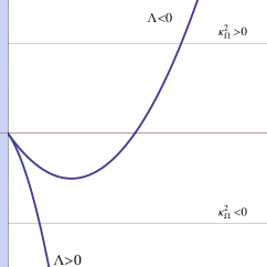
Figure 1: Plot of equation (35), considering different classes of total energy, in the ${\kappa_{\Omega}}^{2}$ parameter. Also, we include two branches in the cosmological constant.

From the figure, that is qualitatively correct for $\gamma\neq 1$, we see that for negative $\Lambda$ all the expanding solutions will re-collapse eventually, regardless of the sign of ${\kappa_{\Omega}}^{2}$. for positive $\Lambda$ an expanding solution will expand forever. We also note that, when ${\kappa_{\Omega}}^{2}<0$, i.e. when the ghost contribution is dominant, there are contracting solutions that reach a minimum and then expand forever, these solutions do not have a big bang singularity.

II.2.1 radiation case, ${\cal G}=X^{2}$

Reproducing the set of equation for this case, we have that the Friedmann like equation is

$$\rm 3\Omega^{\prime 2}-3\beta_{+}^{\prime 2}-3\beta_{-}^{\prime 2}-\frac{3}{4}\phi^{\prime 4}-\rho-\Lambda=0,$$ (36)

and making the same analysis that in the previous case, we have

$$\rm 3\Omega^{\prime 2}=3c_{1}e^{-6\Omega}+3\phi_{1}e^{-4\Omega}+\mu_{\gamma}e^{-3(\gamma+1)\Omega}+\Lambda,\qquad c_{1}=a_{+}^{2}+a_{-}^{2}.\\$$ (37)

also the relation between the anisotropic function $\rm\beta_{\pm}$, (28) are satisfied. In the last equation we have used the equation (13).

Also, we can follow the same structure that for the matter case and following the Hamilton Jacobi analysis, we now that

$$\rho_{a}\sim e^{-6\Omega},\qquad\rho_{\phi}\sim e^{-4\Omega},\qquad\Omega^{\prime 2}\sim 48\Lambda+\phi_{1}e^{-4\Omega}+{\kappa_{\Omega}}^{2}e^{-6\Omega}+b_{\gamma}e^{-3(1+\gamma)\Omega}$$ (38)

and the corresponding ratios are

$$\frac{\rho_{a}}{\rho_{\phi}}\sim e^{-2\Omega},,\qquad\frac{\rho_{a}}{\rho_{\gamma}}\sim e^{3\Omega(\gamma-1)},\qquad\frac{\rho_{a}}{\Omega^{\prime 2}}\sim\frac{1}{{\kappa_{\Omega}}^{2}+48\Lambda e^{6\Omega}+\phi_{1}e^{2\Omega}+b_{\gamma}e^{3(1-\gamma)\Omega}}.$$ (39)

Hence it is necessary to determine when we have an ever expanding universe. Equation (37) in the new variable $\rm V=e^{3\Omega}$

$$\rm 16V^{\prime 2}-b_{\gamma}V^{1-\gamma}-48\Lambda V^{2}-cV^{2/3}={E_{\Omega}}^{2},\qquad{E_{\Omega}}^{2}={\kappa_{+}}^{2}+{\kappa_{-}}^{2}$$ (40)

That is equivalent to the equation of motion in the coordinate $V$ of a particle under the potential $U$ with energy $\rm E={E_{\Omega}}^{2}$, where

$$\rm U(V)=-b_{\gamma}V^{1-\gamma}-48\Lambda V^{2}-cV^{2/3},.$$ (41)

for this case, the qualitative analysis is the same that when ${\cal G}=X$.

In the following we obtain exact solutions in order to gives the volume function V to each case to ${\cal G}=X$.

II.3 Exact Classical solutions

In order to find the solutions for the remaining minisuperspace variables we employ the Einstein-Hamilton-Jacobi equation, which arises by making the identification $\rm\frac{\partial S(\Omega,\beta_{\pm},\phi)}{\partial q^{\mu}}=\Pi_{\mu}$ in the Hamiltonian constraint $\mathcal{H}_{\perp}=0$, which results in

$$\rm\left(\frac{\partial S}{\partial\Omega}\right)^{2}-\left(\frac{\partial S}{\partial\beta_{+}}\right)^{2}-\left(\frac{\partial S}{\partial\beta_{-}}\right)^{2}+\frac{12}{f(\phi)}\left(\frac{\partial S}{\partial\phi}\right)^{2}-b_{\gamma}e^{3\Omega(1-\gamma)}-48\Lambda e^{6\Omega}=0$$ (42)

in order to solve the above equation, we assume a solution of the form $S(\Omega,\beta_{\pm},\phi)=S_{1}(\Omega)+S_{2}(\beta_{+})+S_{3}(\beta_{-})+S_{4}(\phi)$ which results in the following set of ordinary differential equations

$$\rm\left(\frac{dS_{1}}{d\Omega}\right)^{2}-\left(b_{\gamma}e^{-3(\gamma-1)\Omega}+48\Lambda e^{6\Omega}+{\kappa_{\Omega}}^{2}\right)=0$$ (43)

$$\rm\left(\frac{dS_{2}}{d\beta_{+}}\right)^{2}-{\kappa_{+}}^{2}=0$$ (44)

$$\rm\left(\frac{dS_{3}}{d\beta_{-}}\right)^{2}-{\kappa_{-}}^{2}=0$$ (45)

$$\rm\frac{12}{f(\phi)}\left(\frac{dS_{4}}{d\phi}\right)^{2}-{\kappa_{\phi}}^{2}=0.$$ (46)

Here the ${\kappa_{i}}$ are separation constants satisfying the relation ${\kappa_{\Omega}}^{2}={\kappa_{+}}^{2}+{\kappa_{-}}^{2}+{\kappa_{\phi}}^{2}$, ${\kappa_{\pm}}$ are real, ${\kappa_{\phi}}^{2}$ should have the same signs as ${f(\phi)}$ and for consistency with Eq.(17) we have ${\kappa_{\phi}}^{2}=24\eta$. Recalling the expressions for the momenta we can obtain solutions for equations (43-46) in quadrature, in particular

$$\rm\Delta\tau=12\int\frac{d\Omega}{\sqrt{48\Lambda+{\kappa_{\Omega}}^{2}e^{-6\Omega}+b_{\gamma}e^{-3(1+\gamma)\Omega}}}.$$ (47)

$$\rm\Delta\beta_{\pm}=\mp\frac{\kappa_{\pm}}{12}\int e^{-3\Omega(\tau)}d\tau.$$ (48)

We already know the solution for (46). As can be seen from (48), in order to obtain solutions for $\beta_{\pm}$ one needs to find a solution for $\Omega$, which can be obtained from (47).

The equation (47), does not have a general solution, however, it is possible find solutions for particular values of the barotropic parameter $\gamma$ with $\Lambda\not=0$.

1. $\Lambda=0$ and $\gamma\not=1$

   The equation (47) can be written as

   $$\rm d\tau=12\frac{e^{3\Omega}d\Omega}{\sqrt{{\kappa_{\Omega}}^{2}+b_{\gamma}e^{-3\Omega(\gamma-1)}}}.$$ (49)

   when we consider the time transformations $\rm d\tau=e^{3\gamma\Omega}dT$, and the change of variable $\rm u={\kappa_{\Omega}}^{2}+b_{\gamma}e^{-3(\gamma-1)\Omega}$, this equation has the solution

   $$\rm\Omega(T)=Ln\left[\theta_{\gamma}T^{2}+\delta_{\gamma}T\right]^{-\frac{1}{3(\gamma-1)}},$$ (50)

   where $\theta_{\gamma}=\left(\frac{\gamma-1}{8}\right)^{2}b_{\gamma}$ and $\delta_{\gamma}=-\sqrt{{\kappa_{\Omega}}^{2}}\frac{\gamma-1}{4}$. With this, the time transformation becomes

   $$\rm d\tau=\left[\theta_{\gamma}T^{2}+\delta_{\gamma}T\right]^{-\frac{\gamma}{(\gamma-1)}}\,dT.$$

   and the closed form is andrei ,

   $$\tau=\frac{(1-\gamma)}{\delta_{\gamma}}\left[\theta_{\gamma}T^{2}+\delta_{\gamma}T\right]^{\frac{1}{1-\gamma}}\,_{2}F_{1}\left(1,-\frac{2}{\gamma-1};\frac{\gamma-2}{\gamma-1};-\frac{T\theta_{\gamma}}{\delta_{\gamma}}\right),$$ (51)

   here ${}_{2}F_{1}$ is a hypergeometric function. We also have

   $$\rm\rm\int e^{-3\Omega}d\tau=\frac{1}{\delta_{\gamma}}\,Ln\left[\frac{T}{\theta_{\gamma}T+\delta_{\gamma}}\right].$$ (52)

   The anisotropy functions and the scalar field are given by

   $$\rm\Delta\beta_{\pm}=\mp\frac{\kappa_{\pm}}{12\delta_{\gamma}}\,Ln\left[\frac{T}{\theta_{\gamma}T+\delta_{\gamma}}\right].$$ (53)

   $$\rm\phi(T)=\left\{\begin{tabular}[]{ll}$\rm\left[(m+2)\sqrt{\frac{\eta}{2\omega}}\frac{1}{\delta_{\gamma}}\,Ln\left[\frac{T}{\theta_{\gamma}T+\delta_{\gamma}}\right]\right]^{\frac{2}{m+2}}$,&$f(\phi)=\omega\phi^{m},\quad m\not=-2$\\ $\rm Exp\left\{\sqrt{\frac{2\eta}{\omega}}\frac{1}{\delta_{\gamma}}\,Ln\left[\frac{T}{\theta_{\gamma}T+\delta_{\gamma}}\right]\right\}$,&$f(\phi)=\omega\phi^{-2},\quad m=-2$\\ $\rm\frac{2}{m}\,Ln\left[m\sqrt{\frac{\eta}{2\omega}}\frac{1}{\delta_{\gamma}}\,Ln\left[\frac{T}{\theta_{\gamma}T+\delta_{\gamma}}\right]\right]$,&$f(\phi)=\omega e^{m\phi},\quad m\not=0$\\ $\rm\sqrt{2\eta}\frac{1}{\delta_{\gamma}}\,Ln\left[\frac{T}{\theta_{\gamma}T+\delta_{\gamma}}\right]$&$f(\phi)=\omega,\quad m=0$\end{tabular}\right.$$ (54)

   As a concrete example we consider the particular value $\gamma=0$, then $\tau=T$ and $\Omega$ becomes

   $$\rm\Omega(\tau)=Ln\left[\frac{3}{4}\mu_{0}T^{2}+\frac{\sqrt{{\kappa_{\Omega}}^{2}}}{4}T\right]^{\frac{1}{3}},\qquad\Rightarrow\qquad e^{3\Omega}=\frac{3}{4}\mu_{0}T^{2}+\frac{\sqrt{{\kappa_{\Omega}}^{2}}}{4}T$$ (55)

   if isotropization is possible, this volume function would not make it quick, and the integral

   $$\rm\int e^{-3\Omega}d\tau=\frac{4}{\sqrt{{\kappa_{\Omega}}^{2}}}\,Ln\left[\frac{\tau}{\frac{\sqrt{{\kappa_{\Omega}}^{2}}}{4}+\frac{3}{4}\mu_{0}\tau}\right].$$

   So, the classical solutions for the anisotropic function $\beta_{\pm}$ and $\phi$ field are,

   $$\rm\Delta\beta_{\pm}=\mp\frac{\kappa_{\pm}}{3\sqrt{{\kappa_{\Omega}}^{2}}}\,Ln\left[\frac{\tau}{\frac{\sqrt{{\kappa_{\Omega}}^{2}}}{4}+\frac{3}{4}\mu_{0}\tau}\right].$$ (56)

   $$\rm\phi(\tau)=\left\{\begin{tabular}[]{ll}$\rm\left[(m+2)\sqrt{\frac{\eta}{2\omega}}Ln\left[\frac{\tau}{\frac{\sqrt{{\kappa_{\Omega}}^{2}}}{4}+\frac{3}{4}\mu_{0}\tau}\right]\right]^{\frac{2}{m+2}}$,&$f(\phi)=\omega\phi^{m},\quad m\not=-2$\\ $\rm Exp\left\{\sqrt{\frac{2\eta}{\omega}}Ln\left[\frac{\tau}{\frac{\sqrt{{\kappa_{\Omega}}^{2}}}{4}+\frac{3}{4}\mu_{0}\tau}\right]\right\}$,&$f(\phi)=\omega\phi^{-2},\quad m=-2$\\ $\rm\frac{2}{m}\,Ln\left[m\sqrt{\frac{\eta}{2\omega}}Ln\left[\frac{\tau}{\frac{\sqrt{{\kappa_{\Omega}}^{2}}}{4}+\frac{3}{4}\mu_{0}\tau}\right]\right]$,&$f(\phi)=\omega e^{m\phi},\quad m\not=0$\\ $\sqrt{2\eta}\frac{4}{\sqrt{{\kappa_{\Omega}}^{2}}}\,Ln\left[\frac{\tau}{\frac{\sqrt{{\kappa_{\Omega}}^{2}}}{4}+\frac{3}{4}\mu_{0}\tau}\right].$&$f(\phi)=\omega,\quad m=0$\end{tabular}\right.$$ (57)

2. $\Lambda=0$ and $\gamma=1$

   In this case equation (47) is

   $$\rm\Delta\tau=\int\frac{12}{\sqrt{b_{2}e^{-6\Omega}}}d\Omega$$ (58)

   with $\rm b_{2}={\kappa_{\Omega}}^{2}+48\mu_{1}$ that we assume positive. Integrating we obtain

   $$\rm e^{3\Omega}=\frac{\sqrt{b_{2}}\Delta\tau}{4}.$$ (59)

   if isotropization is possible, this volume function would not make it quick. For the anisotropic functions we have

   $$\rm\Delta\beta_{\pm}=\mp\frac{\kappa_{\pm}}{12}\int e^{-3\Omega(\tau)}d\tau=\mp{\kappa_{\pm}}\frac{1}{3\sqrt{b_{2}}}Ln(\Delta\tau),$$ (60)

   and the scalar field is given by

   $$\rm\phi(\tau)=\left\{\begin{tabular}[]{ll}$\rm\left[(m+2)\sqrt{\frac{\eta}{2\omega}}\frac{4}{\sqrt{b_{2}}}Ln(\Delta\tau)\right]^{\frac{2}{m+2}}$,&$f(\phi)=\omega\phi^{m},\quad m\not=-2$\\ $\rm Exp\left\{\sqrt{\frac{2\eta}{\omega}}\frac{4}{\sqrt{b_{2}}}Ln(\Delta\tau)\right\}$,&$f(\phi)=\omega\phi^{-2},\quad m=-2$\\ $\rm\frac{2}{m}\,Ln\left[m\sqrt{\frac{\eta}{2\omega}}\frac{4}{\sqrt{b_{2}}}Ln(\Delta\tau)\right]$,&$f(\phi)=\omega e^{m\phi},\quad m\not=0$\\ $\rm\sqrt{2\eta}\frac{4}{\sqrt{b_{2}}}Ln(\Delta\tau)$,&$f(\phi)=\omega,\quad m=0$\end{tabular}\right.$$ (61)

3. $\Lambda\not=0$ and $\gamma=-1$

   (47) has the form

   $$\rm\Delta\tau=\int\frac{12}{\sqrt{{\kappa_{\Omega}}^{2}e^{-6\Omega}+b_{3}}}d\Omega$$ (62)

   where $\rm b_{3}=48\mu_{-1}+48\Lambda$ .

   $$\rm\Delta\tau=\frac{4}{\sqrt{b_{3}}}\,arccsch\left(\sqrt{\frac{{\kappa_{\Omega}}^{2}}{b_{3}}}e^{-3\Omega}\right)$$ (63)

   solving for $\Omega$

   $$\rm\Omega=\frac{1}{3}Ln\left|\sqrt{\frac{{\kappa_{\Omega}}^{2}}{b_{3}}}\,\sinh\left(\frac{\sqrt{b_{3}}}{4}\Delta\tau\right)\right|$$ (64)

   the inverse volume function is

   $$\rm e^{-3\Omega}=\sqrt{\frac{b_{3}}{{\kappa_{\Omega}}^{2}}}\,csch\left(\frac{\sqrt{b_{3}}}{4}\Delta\tau\right)$$

   if isotropization is possible, the corresponding volume function would make it quick, its integral become

   $$\rm\int e^{-3\Omega}d\tau=\frac{4}{\sqrt{{\kappa_{\Omega}}^{2}}}Ln\left|\tanh\left(\frac{\sqrt{b_{3}}}{4}\Delta\tau\right)\right|$$ (65)

   and as the anisotropic function dependent of this integral, so

   $$\rm\Delta\beta_{\pm}(\tau)=\pm\frac{\kappa_{\pm}}{3\sqrt{{\kappa_{\Omega}}^{2}}}\,Ln\left|\tanh\left(\frac{\sqrt{b_{3}}}{4}\Delta\tau\right)\right|$$ (66)

   Also, the field $\phi$ use this integral (see equation (18), and the corresponding solutions becomes

   $$\rm\phi(\tau)=\left\{\begin{tabular}[]{ll}$\rm\left[-(m+2)\sqrt{\frac{\eta}{2\omega}}\frac{4}{\sqrt{{\kappa_{\Omega}}^{2}}}Ln\left|\tanh\left(\frac{\sqrt{b_{3}}}{4}\Delta\tau\right)\right|\right]^{\frac{2}{m+2}}$,&$f(\phi)=\omega\phi^{m},\quad m\not=-2$\\ $\rm Exp\left\{-\sqrt{\frac{2\eta}{\omega}}\frac{4}{\sqrt{{\kappa_{\Omega}}^{2}}}Ln\left|\tanh\left(\frac{\sqrt{b_{3}}}{4}\Delta\tau\right)\right|\right\}$,&$f(\phi)=\omega\phi^{-2},\quad m=-2$\\ $\rm\frac{2}{m}\,Ln\left[-m\sqrt{\frac{\eta}{2\omega}}\frac{4}{\sqrt{{\kappa_{\Omega}}^{2}}}Ln\left|\tanh\left(\frac{\sqrt{b_{3}}}{4}\Delta\tau\right)\right|\right]$,&$f(\phi)=\omega e^{m\phi},\quad m\not=0$\\ $\rm-\sqrt{2\eta}\frac{4}{\sqrt{{\kappa_{\Omega}}^{2}}}Ln\left|\tanh\left(\frac{\sqrt{b_{3}}}{4}\Delta\tau\right()\right|$&$f(\phi)=\omega,\quad m=0$\end{tabular}\right.$$ (67)

   with the condition $\omega>0$.

   Also we can consider the special case, when $\rm b_{3}=0$ or $\rm\mu_{-1}=-\Lambda$

   $$\rm\Delta\tau = \rm\frac{4}{\sqrt{{\kappa_{\Omega}}^{2}}}e^{3\Omega},$$

   $$\rm\Omega = \rm\frac{1}{3}Ln\left|\frac{\sqrt{{\kappa_{\Omega}}^{2}}}{4}\Delta\tau\right|$$

   we have the following expression

   $$\rm e^{-3\Omega}=\frac{4}{\sqrt{{\kappa_{\Omega}}^{2}}}\frac{1}{\Delta\tau},$$

   the isotropization is possible for this case, because the corresponding volume function would make it quick, its integral become

   $$\rm\int e^{-3\Omega}d\tau=\frac{4}{\sqrt{{\kappa_{\Omega}}^{2}}}Ln\left|\Delta\tau\right|.$$ (68)

   so, the anisotropic function $\beta_{\pm}$ and the $\phi$ function becomes for this case

   $$\rm\Delta\beta_{\pm}(\tau)=\mp\frac{\kappa_{\pm}}{3\sqrt{{\kappa_{\Omega}}^{2}}}Ln\left|\Delta\tau\right|.$$ (69)

   $$\rm\phi(\tau)=\left\{\begin{tabular}[]{ll}$\rm\left[(m+2)\sqrt{\frac{\eta}{2\omega}}\frac{4}{\sqrt{{\kappa_{\Omega}}^{2}}}Ln\left|\Delta\tau\right|\right]^{\frac{2}{m+2}}$,&$f(\phi)=\omega\phi^{m},\quad m\not=-2$\\ $\rm Exp\left\{\sqrt{\frac{2\eta}{\omega}}\frac{4}{\sqrt{{\kappa_{\Omega}}^{2}}}Ln\left|\Delta\tau\right|\right\}$,&$f(\phi)=\omega\phi^{-2},\quad m=-2$\\ $\rm\frac{2}{m}\,Ln\left[m\sqrt{\frac{\eta}{2\omega}}\frac{4}{\sqrt{{\kappa_{\Omega}}^{2}}}Ln\left|\Delta\tau\right|\right]$,&$f(\phi)=\omega e^{m\phi},\quad m\not=0$\\ $\rm\sqrt{2\eta}\frac{4}{\sqrt{{\kappa_{\Omega}}^{2}}}Ln\left|\Delta\tau\right|$&$f(\phi)=\omega,\quad m=0$\end{tabular}\right.$$ (70)

4. $\Lambda\not=0$ and $\gamma=0$

   For this case, equation (47) is

   $$\rm\Delta\tau = \rm\int\frac{12e^{3\Omega}}{\sqrt{{\kappa_{\Omega}}^{2}+48\mu_{0}e^{3\Omega}+48\Lambda e^{6\Omega}}}d\Omega$$ (71)

   $$= \rm\frac{1}{\sqrt{3\Lambda}}Ln\,\left[\frac{b_{0}+96\Lambda e^{3\Omega}}{48\Lambda}+\frac{1}{2\sqrt{3\Lambda}}\sqrt{{\kappa_{\Omega}}^{2}+b_{0}e^{3\Omega}+48\Lambda e^{6\Omega}}\right]$$ (72)

   with $b_{0}=48\mu_{0}$, and $\Lambda>0$.

   The function $\Omega$ become

   $$\rm\Omega=\frac{1}{3}Ln\,\left[\frac{12\Lambda\left(e^{\sqrt{3\Lambda}\Delta\tau}-\frac{b_{0}}{48\Lambda}\right)^{2}-{\kappa_{\Omega}}^{2}}{48\Lambda e^{\sqrt{3\Lambda}\Delta\tau}}\right]$$ (73)

   and we have

   $$\rm e^{-3\Omega} = \rm\frac{48\Lambda\,e^{\sqrt{3\Lambda}\Delta\tau}}{12\Lambda\left(e^{\sqrt{3\Lambda}\Delta\tau}-\frac{b_{0}}{48\Lambda}\right)^{2}-{\kappa_{\Omega}}^{2}}$$

   $$\rm\int e^{-3\Omega}d\tau = \rm-\frac{8}{\sqrt{{\kappa_{\Omega}}^{2}}}arctanh\,\left(2\sqrt{\frac{3\Lambda}{{\kappa_{\Omega}}^{2}}}\left(-\frac{b_{0}}{48\Lambda}+e^{\sqrt{3\Lambda}\Delta\tau}\right)\right)$$ (74)

   also, the isotropization is possible, due that the corresponding volume function would make it quick. For the anisotropic functions $\beta_{\pm}$ we have,

   $$\rm\Delta\beta_{\pm}(\tau)=\pm\frac{2\kappa_{\pm}}{3\sqrt{{\kappa_{\Omega}}^{2}}}\,arctanh\,\left(2\sqrt{\frac{3\Lambda}{{\kappa_{\Omega}}^{2}}}\left(-\frac{b_{0}}{48\Lambda}+e^{\sqrt{3\Lambda}\Delta\tau}\right)\right)$$ (75)

   and for the $\phi$ function

   $$\rm\phi(\tau)=\left\{\begin{tabular}[]{ll}$\rm\left[-(m+2)\sqrt{\frac{\eta}{2\omega}}\frac{8}{\sqrt{{\kappa_{\Omega}}^{2}}}arctanh\,\left(2\sqrt{\frac{3\Lambda}{{\kappa_{\Omega}}^{2}}}\left(-\frac{b_{0}}{48\Lambda}+e^{\sqrt{3\Lambda}\Delta\tau}\right)\right)\right]^{\frac{2}{m+2}}$,&$f(\phi)=\omega\phi^{m},\quad m\not=-2$\\ $\rm Exp\left\{-\sqrt{\frac{2\eta}{\omega}}\frac{8}{\sqrt{{\kappa_{\Omega}}^{2}}}arctanh\,\left(2\sqrt{\frac{3\Lambda}{{\kappa_{\Omega}}^{2}}}\left(-\frac{b_{0}}{48\Lambda}+e^{\sqrt{3\Lambda}\Delta\tau}\right)\right)\right\}$,&$f(\phi)=\omega\phi^{-2},\quad m=-2$\\ $\rm\frac{2}{m}\,Ln\left[-m\sqrt{\frac{\eta}{2\omega}}\frac{8}{\sqrt{{\kappa_{\Omega}}^{2}}}arctanh\,\left(2\sqrt{\frac{3\Lambda}{{\kappa_{\Omega}}^{2}}}\left(-\frac{b_{0}}{48\Lambda}+e^{\sqrt{3\Lambda}\Delta\tau}\right)\right)\right]$,&$f(\phi)=\omega e^{m\phi},\quad m\not=0$\\ $\rm-\sqrt{2\eta}\frac{8}{\sqrt{{\kappa_{\Omega}}^{2}}}arctanh\,\left(2\sqrt{\frac{3\Lambda}{{\kappa_{\Omega}}^{2}}}\left(-\frac{b_{0}}{48\Lambda}+e^{\sqrt{3\Lambda}\Delta\tau}\right)\right)$&$f(\phi)=\omega,\quad m=0$\end{tabular}\right.$$ (76)

5. $\Lambda\not=0$ and $\gamma=1$

   Equation (47) becomes

   $$\rm\Delta\tau=\int\frac{12}{\sqrt{b_{4}e^{-6\Omega}+48\Lambda}}d\Omega$$ (77)

   where $\rm b_{4}={\kappa_{\Omega}}^{2}+48\mu_{1}$. In this case also we have two possible solutions depending on the value of the cosmological constant

   • $\rm\Lambda>0$ .
     The solution become

     $$\rm\Delta\tau=\frac{1}{\sqrt{3\Lambda}}\,arcsinh\,\left(4\sqrt{\frac{3\Lambda}{b_{4}}}e^{3\Omega}\right)$$ (78)

     so, the function $\Omega$ is

     $$\rm\Omega=\frac{1}{3}Ln\left|\frac{1}{4}\sqrt{\frac{b_{4}}{3\Lambda}}\,sinh\,\left(\sqrt{3\Lambda}\Delta\tau\right)\right|$$ (79)

     and

     $$\rm e^{-3\Omega} = \rm 4\sqrt{\frac{3\Lambda}{b_{4}}}\,csch\,\left(\sqrt{3\Lambda}\Delta\tau\right)$$

     $$\rm\int e^{-3\Omega}d\tau = \rm\frac{4}{\sqrt{b_{4}}}\,Ln\left[tanh\,\left(\sqrt{3\Lambda}\Delta\tau\right)\right].$$ (80)

     for this case the isotropization is possible, the corresponding volume function would make it quick. For the anisotropic functions $\beta_{\pm}$ we have

     $$\rm\Delta\beta_{\pm}=\pm\frac{\kappa_{\pm}}{3\sqrt{b_{4}}}Ln\left[tanh\,\left(\sqrt{3\Lambda}\Delta\tau\right)\right]$$ (81)

     and for the $\phi$ field

     $$\rm\phi(\tau)=\left\{\begin{tabular}[]{ll}$\rm\left[-(m+2)\sqrt{\frac{\eta}{2\omega}}\frac{4}{\sqrt{b_{4}}}Ln\left[tanh\,\left(\sqrt{3\Lambda}\Delta\tau\right)\right]\right]^{\frac{2}{m+2}}$,&$f(\phi)=\omega\phi^{m},\quad m\not=-2$\\ $\rm Exp\left\{-\sqrt{\frac{2\eta}{\omega}}\frac{4}{\sqrt{b_{4}}}Ln\left[tanh\,\left(\sqrt{3\Lambda}\Delta\tau\right)\right]\right\}$,&$f(\phi)=\omega\phi^{-2},\quad m=-2$\\ $\rm\frac{2}{m}\,Ln\left[-m\sqrt{\frac{\omega\eta}{2\omega}}\frac{4}{\sqrt{b_{4}}}Ln\left[tanh\,\left(\sqrt{3\Lambda}\Delta\tau\right)\right]\right]$,&$f(\phi)=\omega e^{m\phi},\quad m\not=0$\\ $\rm-\sqrt{2\eta}\frac{4}{\sqrt{b_{4}}}Ln\left[tanh\,\left(\sqrt{3\Lambda}\Delta\tau\right)\right]$&$f(\phi)=\omega,\quad m=0$\end{tabular}\right.$$ (82)

   • $\rm\Lambda<0$ .
     The corresponding solutions are

     $$\rm\Delta\tau=-\frac{1}{\sqrt{3|\Lambda|}}\,arccos\,\left(4\sqrt{\frac{3|\Lambda|}{b_{4}}}\,e^{3\Omega}\right)$$ (83)

     the function $\Omega$

     $$\rm\Omega=\frac{1}{3}Ln\left|\frac{1}{4}\sqrt{\frac{b_{4}}{3|\Lambda|}}cos\,\left(\sqrt{3|\Lambda|}\Delta\tau\right)\right|$$ (84)

     as the volume has an oscillatory behavior, the isotropization do not yield for this case, and for completeness we calculate

     $$\rm e^{-3\Omega} = \rm 4\sqrt{\frac{3|\Lambda|}{b_{4}}}\sec\,\left(\sqrt{3|\Lambda|}\Delta\tau\right)$$

     $$\rm\int e^{-3\Omega}d\tau = \rm\frac{4}{\sqrt{b_{4}}}Ln\left|\sec\left(\sqrt{3|\Lambda|}\,\Delta\tau\right)+\tan\left(\sqrt{3|\Lambda|}\,\Delta\tau\right)\right|$$ (85)

     $$= \rm\frac{4}{\sqrt{b_{4}}}Ln\left|\frac{\cos\left(\frac{\sqrt{3|\Lambda|}}{2}\Delta\tau\right)+\sin\left(\frac{\sqrt{3|\Lambda|}}{2}\Delta\tau\right)}{\cos\left(\frac{\sqrt{3|\Lambda|}}{2}\Delta\tau\right)-\sin\left(\frac{\sqrt{3|\Lambda|}}{2}\right)}\right|,$$

     the anisotropic functions $\beta_{\pm}$,

     $$\rm\Delta\beta_{\pm}=\mp\frac{\kappa_{\pm}}{3\sqrt{b_{4}}}Ln\left|\sec\left(\sqrt{3|\Lambda|}\,\Delta\tau\right)+\tan\left(\sqrt{3|\Lambda|}\,\Delta\tau\right)\right|$$ (86)

     and the $\phi$ field

     $$\rm\phi(\tau)=\left\{\begin{tabular}[]{ll}$\rm\left[(m+2)\sqrt{\frac{\eta}{2\omega}}\frac{4}{\sqrt{b_{4}}}Ln\left|\sec\left(\sqrt{3|\Lambda|}\,\Delta\tau\right)+\tan\left(\sqrt{3|\Lambda|}\,\Delta\tau\right)\right|\right]^{\frac{2}{m+2}}$,&$f(\phi)=\omega\phi^{m},\quad m\not=-2$\\ $\rm Exp\left\{\sqrt{\frac{2\eta}{\omega}}\frac{4}{\sqrt{b_{4}}}Ln\left|\sec\left(\sqrt{3|\Lambda|}\,\Delta\tau\right)+\tan\left(\sqrt{3|\Lambda|}\,\Delta\tau\right)\right|\right\}$,&$f(\phi)=\omega\phi^{-2},\quad m=-2$\\ $\rm\frac{2}{m}\,Ln\left[m\sqrt{\frac{\eta}{2\omega}}\frac{4}{\sqrt{b_{4}}}Ln\left|\sec\left(\sqrt{3|\Lambda|}\,\Delta\tau\right)+\tan\left(\sqrt{3|\Lambda|}\,\Delta\tau\right)\right|\right]$,&$f(\phi)=\omega e^{m\phi},\quad m\not=0$\\ $\rm\sqrt{2\eta}\frac{4}{\sqrt{b_{4}}}Ln\left|\sec\left(\sqrt{3|\Lambda|}\,\Delta\tau\right)+\tan\left(\sqrt{3|\Lambda|}\,\Delta\tau\right)\right|$&$f(\phi)=\omega,\quad m=0$\end{tabular}\right.$$ (87)

III Final remarks

In this work we present the study of the classical cosmological anisotropic Bianchi type I in the K-essence formalism. In previous work made by Chimento and co-research chimento , they present the possible isotropization of this model. Our goal in this work is that we obtain the corresponding classical solutions for a barotropic perfect fluid and cosmological term $\Lambda$ who mimetic the scalar field in equation (1). In the case of $\Lambda=0$ and $\gamma\not=1$ we obtain the solutions in closed form. With this solutions we can validate our qualitative analysis on isotropization of the cosmological model, implying that this become when the volume is large in the corresponding time evolution. So, only one solutions do not present the large volume, when $\Lambda<0$ in stiff matter era in the ordinary matter content. We include a qualitative analysis to Friedmann equation when it is written as an equation for the volume that is equivalent to the equation of motion of a particle under a potential and we conclude the same about the isotropization of this anisotropic model, considering the stiff matter and radiation cases. In the quantum analysis for this model, considering the scalar field, the solutions are similar that those found in the Bianchi type IX cosmological model bianchi-ix , you can see the equation (29). For quantum radiation case, the resulting Wheeler-DeWitt equation appears as fractionary differential equation, and the results will be reported elsewhere.

References

• (1) C. Armendariz-Picon, V. Mukhanov and P.J. Steinbardt, Phys. Lett. 85, 4438 (2000); Phys. Rev. D 63, 103510 (2001).
• (2) N. Bose and A.S. Majumdar, Phys. Rev. D 79, 103517 (2009). A k-essence model of inflation, dark matter and dark energy, [arXiv:0812.4131].
• (3) Josue De-Santiago and Jorge L. Cervantes-Cota, Phys. Rev. D 83, 063502, (2011). Generalizing a Unified Model of Dark Matter, Dark Energy, and Inflation with Non Canonical Kinetic Term
• (4) Josue De-Santiago, Jorge L. Cervantes-Cota, David Wands, Phys. Rev. D 87, 023502 (2013). Cosmological phase space analysis of the $F(X)-V(\phi)$ scalar field and bouncing solutions
• (5) D. Saez and V.J. Ballester, Phys. Lett. A 113, 467 (1986).
• (6) Roland de Putter and Eric V. Linder, Astropart. Phys. 28, 263 (2007). Kinetic k-essence and Quintessence. [arXiv:0705.0400].
• (7) T. Chiba, S. Dutta and R.J. Scherrer, Phys. Rev. D 80, 043517 (2009). Slow-roll k-essence, [arXiv:0906.0628].
• (8) F. Arroja and M. Sasaki, Phys. Rev. D 81, 107301 (2010). A note on the equivalence of a barotropic perfect fluid with a k-essence scalar field, [arXiv:1002.1376].
• (9) L.A. García, J.M. Tejeiro and L. Castañeda, K-essence scalar field as dynamical dark energy, [arXiv:1210.5259].
• (10) N. Bilic,G. Tupper, and R. Viollier, Phys.Lett. B 535, 17 (2002).
• (11) M. Bento, O. Bertolami, and A. Sen, Phys.Rev.D 66, 043507(2002).
• (12) C. Armendariz-Picon, T. Damour and V. Mukhanov, Phys. Lett. B 458, 209 (1999); J. Garriga and V. Mukhanov, Phys. Lett. B 458, 219 (1999).
• (13) E.J. Copeland, M. Sami and S. Tsujikawa, Int. J. Mod. Phys. D 15,1753-1936 (2006). Dynamics of dark energy, [arXiv:hep-th 0603057].
• (14) Luis P. Chimento and Mónica Forte, Phys. Rev. D 73, 063502 (2006), Anisotropic k-essence cosmologies.
• (15) M. Madsen, Class. and Quantum Grav. 5, 627 (1988).
• (16) L.O. Pimentel, Class. and Quantum Grav. 6, L263 (1989).
• (17) M.P. Ryan, Hamiltonian cosmology, (Springer, Berlin, 1972).
• (18) Martinez-Gonzalez E and Sanz J L 1995 Astron. Astrophys. 300 346
• (19) Andrei C. Polyanin and Valentin F. Zaitsev, Handbook of Exact solutions for ordinary differential equations, Second edition, Chapman & Hall/CRC. (2003).
• (20) Abraham Espinoza-García, J. Socorro and Luis O. Pimentel, Int. J. of Theor. Phys. (2014), DOI 10.1007/s10773-014-2102-0, Quantum Bianchi Type IX Cosmology in K-Essence Theory.