Proceedings of ICCSA 2014
Normandie University, Le Havre, France - June 23-26, 2014
DYNAMICS OF MEDIA ATTENTION

Abstract. Studies of human attention dynamics analyses how attention is focused on specific topics, issues or people. In online social media, there are clear signs of exogenous shocks, bursty dynamics, and an exponential or powerlaw lifetime distribution. We here analyse the attention dynamics of traditional media, focussing on co-occurrence of people in newspaper articles. The results are quite different from online social networks and attention. Different regimes seem to be operating at two different time scales. At short time scales we see evidence of bursty dynamics and fast decaying edge lifetimes and attention. This behaviour disappears for longer time scales, and in that regime we find Poissonian dynamics and slower decaying lifetimes. We propose that a cascading Poisson process may take place, with issues arising at a constant rate over a long time scale, and faster dynamics at a shorter time scale.

Keywords. co-occurrence network •  media attention •  attention dynamics •  lifetime •  Poisson process.

1 Introduction

With the arrival of large scale data sets, interest in quantifying human attention rose. It became possible to measure precisely how attention grew and decayed [1]. Moreover, it appeared that many human dynamics showed signs of bursty behaviour: short windows of intense activity with long intermittent time spans of inactivity [2]. The duration a person is active—the time between its first and last occurrence, i.e. its lifetime—seems to decay as an exponential, while the edge lifetime seems to follow a powerlaw distribution [3, 4].

We analyse a large dataset of newspaper articles from traditional printed media. We show that the dynamics of this dataset are different from social media. Our data consist of $140\,263$ newspaper articles from Indonesia from roughly 2004 to 2012, gathered by a news service called Joyo, mainly focussing on political news. We automatically identify entities by using a technique known as named entity recognition, and only retain person names that occur in more documents than on average (we discard organisations and locations) [5]. We then construct a network by creating a node for every person and an edge for each co-occurrence between two persons, and we record the date of the co-occurrence. We only take into account co-occurrences of people in the same sentence, and only about $3.2\%$ of the sentences contain more than one person, so this is relatively restrictive. All time is measured in days, denoted by the symbol $\mathrm{d}$, and we report standard errors for estimations.

2 Results

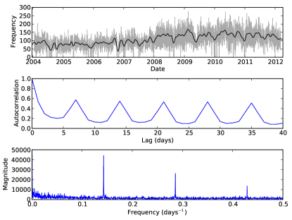
Figure 1: Daily node frequency. The first panel contains the number of nodes in the newspaper (that have at least one co-occurrence) per day (in gray), with the solid black line representing a smoothing (using convolution with a Hann window of 8 weeks) of this daily frequency. The second panel displays the autocorrelation function, which shows a clear peak at a lag of $7$ days, indicating there is a weekly pattern in the data. This is also confirmed by Fourier analysis in the third panel, with a clear peak at a frequency of $$1\text{/}7\text{\,}\mathrm{d}^{-1}$\approx$0.14\text{\,}\mathrm{d}^{-1}$$.

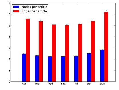
Figure 2: Number of nodes and edges per article per day of the week. The number of nodes count how many nodes appear on average in an article. The number of edges count all the co-occurrences per article. Although the largest part of the cyclical behaviour is due to the weekly newscycle (weekend vs. weekday), there still remains a cyclical pattern after normalisation.

In total, there are $n=9\,467$ nodes and they have about $\langle k_{i}\rangle\approx 12$ neighbours on average. Two people co-occur on average about $3$ times. Let us first look at how these quantities vary over time. Let $E_{t}$ be the number of co-occurrences at time $t$, and $N_{t}$ the number of nodes that have at least one co-occurrence at time $t$. The dynamics of $N_{t}$ follow a distinctive weekly pattern (Fig. 1). This is confirmed by the autocorrelation function, which shows a clear peak at a lag of $7$ days with a correlation of about $0.57$, while the Fourier transform has clear peaks at a frequency of about $$1\text{/}7\text{\,}\mathrm{d}^{-1}$\approx$0.14\text{\,}\mathrm{d}^{-1}$$. Results for $E_{t}$ follow a similar pattern. Although this largely coincides with the weekly cycle of the number of articles, a cyclic pattern remains if the frequencies are normalised by the article frequencies (Fig. 2). For the nodes this pattern is weak, but for the edges more noticeable. Surprisingly, the cycle attains its high point at the end/beginning of the week, while its low point occurs in the middle of the week.

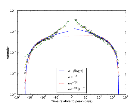
(a) Peak attention

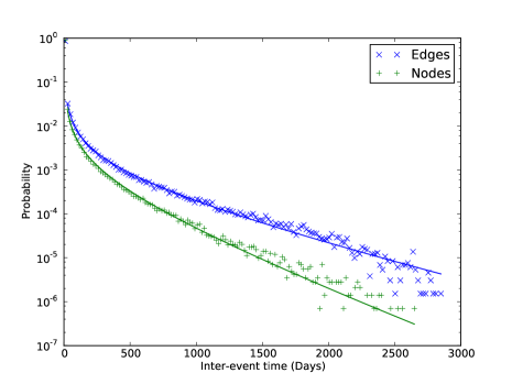
(b) Inter event time

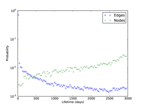
(c) Life time

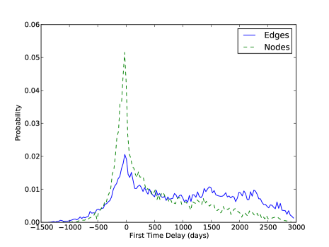
(d) First time delay

Figure 3: Attention statistics. Panel (a) displays how attention—as in the frequency of occurring—grows and decays with the peak attention centred at zero. Panel (b) shows the inter-event time distribution, which has a clear exponential tail, suggesting a Poisson process. Panel (c) features the distribution of the lifetime—the amount of time between the first and last time of observing that node or edge. The edge lifetime decays very fast for the first few days, but then decays much slower. The node lifetime follows an increasing distribution, indicating they can have a very long lifetime. Finally, panel (d) shows the distribution of the first time delay. This delay represents the difference between the time at which we would expect to first observe a node (or edge) and the time at which we actually observed it in the dataset. This suggests that new nodes and edges continuously appear in the media.

Let us denote by $N_{t}(i)$ the number of co-occurrences of node $i$ with any other node at time $t$. The attention for neighbours of $i$ follows a similar pattern as node $i$, more than compared to the overall trend. So, attention for people that co-occur rises and falls together, hinting at some underlying commonality. One possibility is that people occur mostly in regard to a specific issue. The attention of that issue then presumably correlates with the attention of the people playing a role in that issue, resulting in similar patterns of attention.

	Model	$\alpha-\beta\log|t|$	$\alpha|t|^{-\beta}$	$\alpha e^{-\beta t}$	$\alpha e^{-\beta|t|}|t|^{-\gamma}$
Growth	$\alpha$	$0.011\pm 6.9\cdot 10^{-5}$	$0.031\pm 3.2\cdot 10^{-4}$	$0.0056\pm 6.3\cdot 10^{-5}$	$0.0233\pm 1.9\cdot 10^{-4}$
	$\beta$	$0.0013\pm 9.8\cdot 10^{-6}$	$0.49\pm 2.3\cdot 10^{-3}$	$0.0019\pm 3.1\cdot 10^{-5}$	$6.6\cdot 10^{-4}\pm 1.2\cdot 10^{-5}$
	$\gamma$	$-$	$-$	$-$	$0.36\pm\cdot 2.3\cdot 10^{-3}$
	$\Delta\text{AIC}$	$3\,117$	$3\,045$	$4\,883$	$-$
Decay	$\alpha$	$0.014\pm 8.1\cdot 10^{-5}$	$0.037\pm 3.8\cdot 10^{-4}$	$0.0067\pm 7.1\cdot 10^{-5}$	$0.028\pm 2.3\cdot 10^{-4}$
	$\beta$	$0.0017\pm 1.1\cdot 10^{-5}$	$0.46\pm 2.1\cdot 10^{-3}$	$0.0015\pm 2.3\cdot 10^{-5}$	$5.5\cdot 10^{-4}\pm 9.8\cdot 10^{-6}$
	$\gamma$	$-$	$-$	$-$	$0.34\pm 2.2\cdot 10^{-3}$
	$\Delta\text{AIC}$	$2\,559$	$2\,986$	$4\,820$	$-$

Table 1: Growth and decay estimates and model performance. The AIC differences are high, and show that the powerlaw with exponential cut-off $\alpha e^{-\beta|t|}|t|^{-\gamma}$ is the best model.

Let $t_{p}(i)=\operatorname{arg\,max}_{t}N_{t}(i)$ be the peak of the number of co-occurrences of node $i$ with any other node (if there are multiple such times the first is used). We normalise the time series, such that the peak is centred at $0$ with a value of $1$, and denote the average of these time series by $\tilde{N}_{t}$ (see Fig. 3a). Hence $\tilde{N}_{0}=1$, and we are interested in how $\tilde{N}_{t}$ grows for $t<$0\text{\,}\mathrm{d}$$ and decays for $t>$0\text{\,}\mathrm{d}$$. Crane and Sornette [1] proposed that $\tilde{N}_{t}\sim|t|^{-\beta}$, where different exponents $\beta$ would correspond to different universal classes [1]. However, Leskovec et al. [6] found that $\tilde{N}_{t}\sim-\beta\log|t|$, which is unrealistic for large times since $-\log|t|<$0\text{\,}\mathrm{d}$$ for sufficiently large $t$. Alternatively, if the rate of growth/decay would be constant over time, we would expect to see exponential growth and decay $\tilde{N}_{t}\sim e^{-\beta|t|}$.

However, we find that none of these satisfactorily model the growth and decay of attention (we use non-linear least squares for fitting). The logarithmic and exponential functions grow/decay too slowly at a small time (around $10$–$30$ days), while the powerlaw poorly fits the dynamics for larger times. Given that the powerlaw fits the short time scale relatively well, and the longer time scales are better fit by an exponential function, a powerlaw with exponential cut-off $\tilde{N}_{t}\sim e^{-\beta|t|}|t|^{-\gamma}$ seems a reasonable alternative. Indeed, this functional form accurately captures the growth and decay in our data. For determining which model is a better fit, we use Akaike’s Information Criterion (AIC) values, for which a lower value indicates a better fit [7]. We only give the AIC values relative to the minimum, which clearly demonstrates that the powerlaw with exponential cut-off is the best candidate (see Table 1 for results). Obviously, the powerlaw diverges for $|t|\to$0\text{\,}\mathrm{d}$$ so that it seems as if the attention is going to diverge, even though we know it is not (because $\tilde{N}_{0}=1$), and the fitting is done for $|t|>$0\text{\,}\mathrm{d}$$.

Although there is a large degree of symmetry—which Crane and Sornette [1] see as characteristic of endogenous dynamics—we do find different exponents for the growth and decay (see Table 1). In particular, the decay seems slower than the growth at short time scales, and nodes tend to occur more frequently after their peak than before their peak on longer time scales. This contrasts with the findings of Leskovec et al. [6], where the decay was faster than the growth, and attention was lower after the peak than before the peak.

Let $t_{s}(i,j)$ be the time of the $s^{\text{th}}$ co-occurrence between node $i$ and $j$. The inter-event time can be denoted by $\delta_{s}(i,j)=t_{s+1}(i,j)-t_{s}(i,j)$, which can possibly be $0$ if two (or more) co-occurrences happened at the same day. Similarly for nodes, we denote by $t_{s}(i)$ the time of the $s^{\text{th}}$ co-occurrence of $i$ with another node, and by $\delta_{s}(i)=t_{s+1}(i)-t_{s}(i)$ the inter-event time. If events happen at a constant rate, we would expect an exponential distribution of inter-event times. If events follow a bursty patter, we expect to find a powerlaw inter-event time distribution, often observed in other settings [2]. We find that although the probability of inter-event times decays quite fast at a short time scale, the inter-event times for a longer time scale follow an exponential distribution (Fig. 3b). Altogether, a powerlaw with exponential cutoff $p(x)\sim x^{-\alpha}e^{-\beta x}$ provides a better fit than a powerlaw or exponential distribution (log-likelihood ratios $6.3\cdot 10^{4}$ and $3\cdot 10^{4}$ respectively). We employed maximum likelihood estimation (MLE) for the parameters as recommended by Clauset et al. [8]. For the edges, we find coefficients $\alpha\approx 1.003\pm 2.6\cdot 10^{-3}$ and $\beta\approx 0.00151\pm 1.1\cdot 10^{-5}$, while for the nodes the distribution is slightly less skewed, but decays slightly faster, with $\alpha=1.045\pm 3.7\cdot 10^{-3}$ and $\beta=0.00244\pm 2.3\cdot 10^{-5}$, both with a lower cutoff of $x_{\text{min}}=$10\text{\,}\mathrm{d}$$. Indeed, for even shorter time intervals, the decay is very fast, and using lower $x_{\text{min}}$ gives poorer fits.

One explanation is that if somebody is involved in an issue, his co-occurrence shows a bursty pattern at this shorter time scale, but that issues appear at a steady rate over a longer time scale. This could perhaps be modelled as a cascading Poisson process [2], where the rise of an issue triggers the individual events of co-occurrence.

We denote by $\Delta(i,j)=\max t_{s}(i,j)-\min t_{s}(i,j)$ the lifetime of an edge, and similarly by $\Delta(i)$ the lifetime of a node (Fig. 3c). Most edges have a very low lifetime of only a single day, and the probability to have a larger lifetime quickly decreases. Nonetheless, after an initial rapid decay, the probability decays much slower. So, besides the more volatile short term links, there are also many long term stable links. The node lifetimes are rather unusually distributed. Although there are nodes that have a lifetime that is quite short, nodes tend to have a longer lifetime, only cutoff by the duration of the dataset. The lifetime of nodes can thus be long, and can easily run in the decades.

Our data start in about $2004$, but of course some people already appeared in the media earlier than that. That does not imply we will immediately observe them the first day (17 January 2004 to be precise), and it may take days, weeks or perhaps even months before we first observe someone. However, if their process of occurring in the media is stationary, we can calculate the expected time until we first observe them, based on the inter-event time distribution: $\langle t_{0}(i)\rangle=\frac{\langle\delta_{s}(i)^{2}\rangle}{2\langle\delta_{s}(i)\rangle}$ (and similarly so for edges) [9]. We call the difference $\Delta t_{0}(i)=t_{0}(i)-\langle t_{0}(i)\rangle$ the “first time delay”, and if people already appeared in the news before $2004$, we should find that $\Delta t_{0}(i)\approx$0\text{\,}\mathrm{d}$$ for those people. If $\Delta t_{0}(i)$ is much larger for somebody, it becomes unlikely that this person appeared in the news prior to $2004$ (still assuming the process is stationary). The distribution of the first time delay is displayed in Fig. 3d. First, there is a clear peak around $\Delta t_{0}(i)=0$, suggesting that these nodes indeed already appeared in the news prior to $2004$. The fast decay that is visible on the negative part, does not show at the positive part. This implies that many nodes and edges are first observed much later than expected. Hence, new nodes and edges continuously appear in the news. This is especially prominent for the edges, which show an almost uniform distribution between $250$–$2\,000$ days of difference, whereas the distribution for the nodes decays more gradually.

3 Conclusion

Online social media show signs of exogenous shocks, bursty dynamics and exponential lifetime distributions. We have shown here that traditional media work differently, with different regimes operating at two different time scales. There is a short time scale at which links have short lifetime, attention decays quickly and there are indications of burstiness. However, at a longer time scale nodes and links have a relatively long lifetime, attention decays slower, and inter-event times decay exponentially. We believe that this might be modelled as a cascading Poisson process [2]. Issues would arise at a steady rate, triggering individual events of co-occurrence. The longer time scale would be related to the slower dynamics of how issues appear and disappear, while the faster dynamics at a shorter time scale would be due to the individual events within an issue. We aim to further pursue this idea in future research.

References

- Crane and Sornette [2008] R. Crane and D. Sornette. Proc. Natl. Acad. Sci. USA, 105(41):15649–15653 (2008).
- Malmgren et al. [2008] R. D. Malmgren, D. B. Stouffer, A. E. Motter, and L. A. N. Amaral. Proc. Natl. Acad. Sci. USA, 105(47):18153–18158 (2008).
- Hidalgo and Rodriguez-Sickert [2008] C. A. Hidalgo and C. Rodriguez-Sickert. Physica A, 387(12):3017–3024 (2008).
- Leskovec et al. [2008] J. Leskovec, L. Backstrom, R. Kumar, and A. Tomkins. In Proceedings of the 14th ACM SIGKDD International Conference on Knowledge Discovery and Data Mining, KDD ’08, pages 462–470. ACM, New York, NY, USA (2008).
- Finkel et al. [2005] J. R. Finkel, T. Grenager, and C. Manning. In Proceedings of the 43rd Annual Meeting on Association for Computational Linguistics, ACL ’05, pages 363–370. Association for Computational Linguistics, Stroudsburg, PA, USA (2005).
- Leskovec et al. [2009] J. Leskovec, L. Backstrom, and J. Kleinberg. In Proceedings of the 15th ACM SIGKDD International Conference on Knowledge Discovery and Data Mining, KDD ’09, pages 497–506. ACM, New York, NY, USA (2009).
- Burnham and Anderson [2013] K. P. Burnham and D. R. Anderson. Model Selection and Multimodel Inference: A Practical Information-Theoretic Approach. Springer, New York (2013).
- Clauset et al. [2009] A. Clauset, C. R. Shalizi, and M. E. J. Newman. SIAM Rev. Soc. Ind. Appl. Math., 51(4):661–703 (2009).
- Lawler [1995] G. F. Lawler. Introduction to Stochastic Processes. CRC Press (1995).