$X_{max}^{\mu}$ vs. $N^{\mu}$ from Extensive Air Showers as estimator for the mass of primary UHECR’s. Application for the Pierre Auger Observatory.

Abstract

We study the possibility of primary mass estimation for Ultra High Energy Cosmic Rays (UHECR’s) using the $X_{max}^{\mu}$ (the height where the number of muons produced on the core of Extensive Air Showers (EAS) is maximum) and the number $N^{\mu}$ of muons detected on ground. We use the 2D distribution - $X_{max}^{\mu}$ against $N^{\mu}$ in order to find its sensitivity to the mass of the primary particle. For that, we construct a 2D Probability Function $Prob(p,Fe\ |\ X_{max}^{\mu},N^{\mu})$ which estimates the probability that a certain point from the plane $(X_{max}^{\mu}$, $N^{\mu})$ corresponds to a shower induced by a proton, respectively an iron nucleus. To test the procedure, we analyze a set of simulated EAS induced by protons and iron nuclei at energies of $10^{19}eV$ and $20^{\circ}$ zenith angle with CORSIKA. Using the Bayesian approach and taking into account the geometry of the infill detectors from the Pierre Auger Observatory, we observe an improvement in the accuracy of the primary mass reconstruction in comparison with the results obtained using only the $X_{max}^{\mu}$ distributions.

1 Introduction

Nowadays, many experiments try to answer the fundamental questions about the origin, acceleration mechanism, propagation, mass composition and energy spectrum of UHECR’s. One of these experiments is the Pierre Auger Observatory, located in Southern hemisphere in Argentina and dedicated to measure the proprieties of EAS induced by particles with energies greater than $10^{18}eV$. In this work we focus on a method by which one can reconstruct the mass of the primary UHECR using the surface detectors (SD) from the Pierre Auger Observatory which have a duty cycle of about $100\%$.

2 Muon arrival times from EAS

This method has been previously proposed in Rebel et al. (1995); Brancus et al. (2003); Haeusler et al. (2002); Cazon et al. (2005). The idea is to reconstruct the longitudinal profile of the muons produced on the shower core considering the times when the muons reach the ground relative to the shower core. Due to the larger cross section of the primary iron nuclei when compared to primary protons at the same energy, it is obvious that the $<X_{max}^{\mu}>$ for protons is greater than the $<X_{max}^{\mu}>$ for iron induced showers. In Fig. 1 we have represented the coordinate system of the shower axis, which is the same as the one used in the CORSIKA code Heck and Knapp (1989); Heck et al. (1998).We can calculate the time $t_{0}$ between the primary interaction ($P$) and the time when the muon is produced ($A$) Arsene et al. (2012):

$${t_{0}}=\frac{(OB)^{2}-2c(OB)t_{c}\cdot cos\delta+c^{2}t_{c}^{2}-c^{2}t_{\mu}^{2}}{2c(ct_{c}-ct_{\mu}-(OB)cos\delta)}$$ (1)

where $c$ represents the speed of light, $t_{c}$ and $t_{\mu}$ represent the time when the shower core respectively the muon reaches the ground. Having the distribution of the heights at which all the muons were produced, we can transform it in units of $g/cm^{2}$ and then fiting with the Gaisser-Hillas function, the $X_{max}^{\mu}$ value can be obtained.

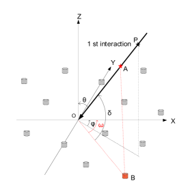
Figure 1: Coordinates system according with those from CORSIKA.

3 Results: $X_{max}^{\mu}$ vs. $N^{\mu}$ sensitivity to the primary mass

We performed a set of CORSIKA simulations containing 60 EAS induced by protons and 60 EAS induced by iron nuclei, at energies $E=10^{19}eV$, zenith angle $\theta=20^{\circ}$, using the QGSJET-II Ostapchenko (2006) hadronic interaction model at the highest energies and taking into account the conditions from the Pierre Auger Observatory (observational plane, magnetic field, etc.). Using the method described above, Fig. 2 shows the reconstructed longitudinal profiles of the muons produced on the shower core considering different distances from the shower axis in observational plane.

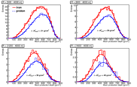
Figure 2: Longitudinal profile of muon production depth evaluated for different intervals of distances from shower axis. Average over 60 CORSIKA simulations per case. We considered only the muons which hit the infill detectors of the Pierre Auger Observatory. The continuous line represents the fit with the Gaisser-Hillas function.

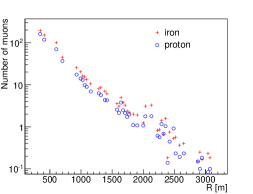
Figure 3: Number of muons produced on the shower core vs. the distance from the shower axis in the observational plane. Average over 60 CORSIKA simulations per case. We considered only the muons which hit the infill detectors of the Pierre Auger Observatory.

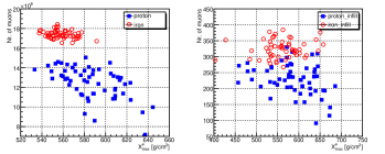
Figure 4: Event by event analysis, number of muons at ground level vs. $X_{max}^{\mu}$, 60 CORSIKA simulations per case. Ideal case, when considering all the muons produced on the shower core at ground level (left), infill case when considering only the muons which hit the infill detectors (right)

.

It can be seen when using the muons from larger distances from the shower axis for the muon production depth (MPD) reconstruction, the difference between the maximum of the profiles tends to increase. In Fig. 3, the number of muons produced on the shower core which reach the infill detectors is represented against the distance from the shower axis in observational plane for the protons, respectively iron nuclei induced showers in the same conditions. The larger number of muons on the ground for the case of iron nuclei as primary particle is due to the higher multiplicity at the first interaction when compared with the primary proton case. The dependence $X_{max}^{\mu}$ vs. $N^{\mu}$ is represented in Fig. 4. Having these two complementary informations $X_{max}^{\mu}$ and $N^{\mu}$ we define a 2D Probability Function $Prob(p,Fe\ |\ X_{max}^{\mu},N^{\mu})$ which estimates the probability that a certain point from the plane $(X_{max}^{\mu}$, $N^{\mu})$ corresponds to a shower induced by a proton, respectively an iron nucleus:

$$Prob(X_{max}^{\mu},N^{\mu}\ |\ p,Fe)=C\cdot exp\left(-\frac{(X_{max}^{\mu}-<X_{max}^{\mu}>)^{2}}{2\sigma_{X_{max}^{\mu}}^{2}}\right)\cdot exp\left(-\frac{(N^{\mu}-<N^{\mu}>)^{2}}{2\sigma_{N^{\mu}}^{2}}\right).$$ (2)

The fit parameters of the function are listed in Table 1. Because the amplitude of the $Prob(X_{max}^{\mu},N^{\mu}\ |\ p,Fe)$ function depends on the ratio of the different species of nuclei in nature (in our particular case, the ratio of primary iron / protons), we use the Bayesian approach to test the reconstruction accuracy of the method.

	$C$	$<X_{max}^{\mu}>$	$\sigma_{X_{max}^{\mu}}$	$<N^{\mu}>$	$\sigma_{N^{\mu}}$
p, ideal	$5.53\pm 1.07$	$572.7\pm 18.07$	$50\pm 22.6$	$1.22\pm 0.3\times 10^{7}$	$1.66\pm 0.33\times 10^{6}$
Fe, ideal	$35.34\pm 6.23$	$557.1\pm 2.06$	$13.75\pm 1.47$	$1.73\pm 0.01\times 10^{7}$	$5.48\pm 0.04\times 10^{5}$
p, infill	$3.32\pm 0.7$	$622.9\pm 14.02$	$35\pm 2.74$	$221.5\pm 10.15$	$35\pm 3.34$
Fe, infill	$4.47\pm 1.34$	$569.4\pm 14.78$	$25\pm 1$	$321.5\pm 6.14$	$28.01\pm 17.06$

Table 1: Parameter values obtained after the fit of the distributions $X_{max}^{\mu}\ vs.\ N^{\mu}$ from Fig. 4 with the 2D Probability Function Eq. 2.

4 Bayesian approach to test the procedure

To test this procedure we need to define certain Prior probabilities and then calculate the Posterior probabilities that a certain point from the plane $(X_{max}^{\mu}$, $N^{\mu})$ corresponds to a shower induced by a proton or an iron nucleus. We know from the simulations $Prob(X_{max}^{\mu},N^{\mu}\ |\ p,Fe)$ (the probability to have the point with the coordinates $X_{max}^{\mu}$ and $N^{\mu}$ if the primary particle was proton or an iron nucleus). Supposing certain Prior probabilities $Prob_{i}(p)$ and $Prob_{i}(Fe)$ which represents the ratio abundance of the primary protons and iron nuclei, we can calculate the Posterior probabilities:

$$Prob_{a}(p\ |\ X_{max}^{\mu},N^{\mu})=K\cdot Prob(X_{max}^{\mu},N^{\mu}\ |\ p)\cdot Prob_{i}(p),$$ (3)

$$Prob_{a}(Fe\ |\ X_{max}^{\mu},N^{\mu})=K\cdot Prob(X_{max}^{\mu},N^{\mu}\ |\ Fe)\cdot Prob_{i}(Fe),$$ (4)

where the constant $K$ can be calculated from the normalization:

$$Prob_{a}(p\ |\ X_{max}^{\mu},N^{\mu})+Prob_{a}(Fe\ |\ X_{max}^{\mu},N^{\mu})=1.$$ (5)

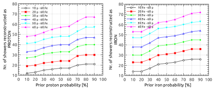
Figure 5: Potential mass discrimination of the method. Number of showers reconstructed as ”PROTON” (left) and ”IRON” (right) for different prior probabilities and different mixtures of showers. Only the muons which entered in the infill detectors were taken into account.

Fig. 5 shows how many showers are reconstructed to be induced by protons respectively iron nuclei, considering different prior probabilities and different combinations of number of showers. In order to see the difference in the accuracy of the reconstruction methods, we consider the particular case with 60 proton induced showers and 60 iron induced showers, with the prior probabilities $Prob_{i}(p)=Prob_{i}(Fe)=50\%$. Let’s consider $Prob_{p\rightarrow p}$ to be the probability for proton induced showers to be reconstructed as ”PROTON”, respectively $Prob_{Fe\rightarrow Fe}$ the probability for iron induced showers to be reconstructed as ”IRON”. The comparison of the reconstruction accuracy of these two methods for this particular case can be seen in Table 2.

	$<X_{max}^{\mu}>$	($<X_{max}^{\mu}>vs.N^{\mu}$)
$Prob_{p\rightarrow p}$	$43.7\pm 2.8\%$	$81.2\pm 32.3\%$
$Prob_{Fe\rightarrow Fe}$	$57.9\pm 2\%$	$84.3\pm 30.3\%$

Table 2: Reconstruction accuracy of the methods $<X_{max}^{\mu}>$ and ($<X_{max}^{\mu}>vs.N^{\mu}$)

5 Conclusions

We observed an improvement in the accuracy of the reconstruction of the primary UHECR’s mass using the 2D Probability Function $Prob(X_{max}^{\mu},N^{\mu}\ |\ p,Fe)$ in comparison with the results obtained only with the $X_{max}^{\mu}$ distributions. Using this method with the surface detectors from the PAO, the duty cycle will be about $100\%$, and will considerably increase the statistics of the events with $E>10^{19}eV$. This method will also be useful when searching for the quantum black holes signature proposed in Arsene et al. (2013).

References

- Rebel et al. (1995) H. Rebel, G. Voelker, M. Foeller, and A. Chilingarian, J.Phys. G21, 451–472 (1995).
- Brancus et al. (2003) I. Brancus, H. Rebel, A. Badea, A. Haungs, C. Aiftimiei, et al., J.Phys. G29, 453–474 (2003).
- Haeusler et al. (2002) R. Haeusler, A. Badea, H. Rebel, I. Brancus, and J. Oehlschlager, Astropart.Phys. 17, 421–426 (2002).
- Cazon et al. (2005) L. Cazon, R. Vazquez, and E. Zas, Astropart.Phys. 23, 393–409 (2005), astro-ph/0412338.
- Heck and Knapp (1989) D. Heck, and J. Knapp, Report FZKA 6097 (1998), Forschungszentrum Karlsruhe; available from http://www-ik.fzk.de/~heck/publications/ (1989).
- Heck et al. (1998) D. Heck, J. Knapp, J. Capdevielle, G. Schatz, and T. Thouw, Report FZKA 6019 (1998), Forschungszentrum Karlsruhe; available from http://www-ik.fzk.de/corsika/physicsdescription/corsikaphys.html (1998).
- Arsene et al. (2012) N. Arsene, H. Rebel, and O. Sima, AIP Conf.Proc. 1498, 304–308 (2012).
- Ostapchenko (2006) S. Ostapchenko, Nucl.Phys.Proc.Suppl. 151, 143–146 (2006), hep-ph/0412332.
- Arsene et al. (2013) N. Arsene, L. I. Caramete, P. B. Denton, and O. Micu (2013), hep-ph/1310.2205.