Comparing Simple Quasar Demographics Models

Abstract

This paper explores several simple model variations for the connections among quasars, galaxies, and dark matter halos for redshifts $1<z<6$. A key component of these models is that we enforce a self-consistent black hole (BH) history by tracking both BH mass and BH growth rate at all redshifts. We connect objects across redshift with a simple constant-number-density procedure, and choose a fiducial model with a relationship between BH and galaxy growth rates that is linear and evolves in a simple way with redshift. Within this fiducial model, we find the quasar luminosity function (QLF) by calculating an “intrinsic” luminosity based on either the BH mass or BH growth rate, and then choosing a model of quasar variability with either a lognormal or truncated power-law distribution of instantaneous luminosities. This gives four model variations, which we fit to the observed QLF at each redshift. With the best-fit models in hand, we undertake a detailed comparison of the four fiducial models, and explore changes to our fiducial model of the BH-galaxy relationship. Each model variation can successfully fit the observed QLF, the shape of which is generally set by the “intrinsic” luminosity at the faint end and by the scatter due to variability at the bright end. We focus on accounting for the reasons that physically different models can make such similar predictions, and on identifying what observational data or physical arguments are most essential in breaking the degeneracies among models.

1 Introduction

Quasars are an important component of modern astrophysics, from their role as extremely luminous objects useful for high redshift surveys to their apparent influence on galaxy formation (see e.g. the recent reviews of Alexander & Hickox, 2012; Kormendy & Ho, 2013). Many phenomenological models have arisen to desribe the connections among quasars, the black holes (BHs) that power them, and their host galaxies and dark matter halos (e.g. Efstathiou & Rees, 1988; Carlberg, 1990; Wyithe & Loeb, 2002, 2003; Haiman, Ciotti & Ostriker, 2004; Marulli et al., 2006; Lidz et al., 2006; Croton, 2009; Shen, 2009; Booth & Schaye, 2010). Despite active research and a wealth of observational data, a single picture of quasar demographics has yet to emerge.

Two recent models in particular have explored simple connections between quasar activity and host galaxy properties. In Conroy & White (2013), hereafter abbreviated “CW13”, the model began by assuming a linear relationship between BH mass and host galaxy mass, and calculated quasar luminosities by assuming a single, mass-independent duty cycle and Eddington ratio with some lognormal scatter. In Hickox et al. (2014), hereafter abbreviated “H14”, a very similar model assumed a linear relationship between average BH accretion rate and galaxy star formtion rate, and then found the quasar luminosity function (QLF) by assuming a truncated power-law distribution of instantaneous accretion rates and a constant radiative efficiency. Both models, despite different perspectives on the BH-galaxy connection and different assumptions about quasar variability, were successful in explaining the basic properties of the observed QLF, along with other observed quasar properties.

This paper aims to connect these models in a self-consistent framework that tracks both BH mass and BH growth across redshift. With both BH masses and average BH accretion rates in hand, we can make a direct comparison between model types. The “model space” we consider has, effectively, three “dimensions”: the choice of BH-galaxy relationship (including redshift evolution), the choice of whether to connect quasar activity to BH masses or average BH accretion rates, and the choice of quasar variability model. To facilitate the exploration of this model space, we will make use of simplifying assumptions wherever possible, while being mindful of where such simplifications may not apply. In particular, our assumptions about redshift evolution begin to break down at low redshift, so we will restrict ourselves to the redshift range $1<z<6$. In this range, there is much data available from large-scale (wide area, high redshift) optical surveys (e.g. Wolf et al., 2003; Richards et al., 2006; Croom et al., 2009; Willott et al., 2010; Ikeda et al., 2011; Masters et al., 2012; McGreer et al., 2013; Ross et al., 2013), which makes the QLF for optical (type-I) quasars a useful observable to choose as the “input” for setting the best-fit parameters of each model variation.

Section 2 of this paper describes our fiducial model and variations in detail; section 3 compares the success of each fiducial model variation in fitting the observed QLF; section 4 explores variations beyond our fiducial model; and section 5 summarizes the major conclusions and implications of our results. Where necessary, we use a $\Lambda$CDM cosmology with $\Omega_{M}=0.28$ and $\Omega_{\Lambda}=0.72$, and assume $h=0.7$. Stellar masses assume a Chabrier (2003) initial mass function. Unless specificed otherwise, the $\log$ of any quantity is taken to be $\log_{10}$.

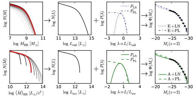
Figure 1: A schematic look at our model. The left column shows the BH properties (mass in the top panel, average growth rate in the bottom panel) for our fiducial “growth-based evolution” model of the BH-galaxy relationship. All of our observed redshifts are shown (see figure 2 for the full list), with black at the lowest redshift ($z=1$) and lightest gray at the highest redshift ($z=6$). The remaining columns show only $z=2$, which is highlighted in red in the first column. The second column shows the “intrinsic” QLF used in the “Eddington model” (top panel) and “accretion model” (bottom panel). These are simply the same curves from the left column, expressed in units of luminosity. The third column shows the distribution of observed luminosities (in units of “intrinsic” luminosity). The right column shows the results of convolving the “intrinsic” QLF in the second column with the distributions in the third column. This gives four model variations: E+LN, the dotted blue line, is the Eddington model convolved with $P_{\rm LN}$; E+PL, the dash-dotted blue line, is the Eddington model convolved with $P_{\rm PL}$; A+LN, the solid green line, is the accretion model convolved with $P_{\rm LN}$; A+PL, the dashed green line, is the accretion model convolved with $P_{\rm PL}$. See table 1 for a summary of the terminology.

2 The model

2.1 Galaxy mass and growth rate

Our model begins with the halo mass functions (HMFs) from the fitting functions of Tinker et al. (2008, 2010). These are translated into galaxy stellar mass functions (SMFs) using the empirically constrained stellar mass-halo mass relations from Behroozi et al. (2013). These relations are calculated along with two components of scatter, an “intrinsic” scatter and “observational” scatter. For our purposes, we convolve the SMF with only the “intrinsic” scatter, since we are not interested in a direct comparison to the observed SMF.

These first steps are the same as the ones taken in CW13, but we add the additional calculation of finding the mass growth rate of galaxies across redshift. We will sometimes refer to this as the star formation rate (SFR), although equating net mass growth with star formation is only an approximation. The true SFR differs from the net mass growth due to factors such as stellar mass loss and merging, which are discussed in Behroozi et al. (2013) but which we do not consider in detail in this paper. To connect the SMFs across redshift, we use a matching procedure that assumes the galaxy masses preserve rank order, and each galaxy maintans a position in the SMF with constant number density. With this assumption, we can obtain the galaxy growth rates at each redshift using a simple central-difference approximation. At very high masses, this yields a negative growth (which we set to zero for the purposes of the model), indicating that our assumptions are not accurate for such extreme objects. For low redshift, this negative growth impacts more galaxies (all those above $10^{11}M_{\odot}$ for $z=1$), so we restrict our analysis to the range $1<z<6$.

2.2 Black hole-galaxy relations

With a stellar mass history for each galaxy in hand, we must now decide how to relate galaxies to their central BHs. To begin we neglect scatter in the BH-galaxy relationship, which allows us to directly apply our matching procedure across redshifts to the BHs as well as the galaxies, without introducing additional complications.

Our fiducial model assumes a linear relationship between BH and galaxy growth rates, similar to H14, but adds a scaling with redshift similar to what was used in CW13.

$$\langle\dot{M}_{\rm BH}\rangle =10^{-3.5}\dot{M}_{\rm gal}(1+z)^{2}$$ (1)

$$\implies\langle\dot{M}_{\rm BH}\rangle =10^{\alpha_{G}}\dot{M}_{\rm gal}$$ (2)

$$\text{where}\;\alpha_{G}(z) \equiv-3.5+2\log(1+z)$$ (3)

Where we implicitly assume that $\alpha_{G}$ is independent of mass for this model. The choice of a local value of $\alpha_{G}=-3.5$ is motivated by observations such as Rafferty et al. (2011), Mullaney et al. (2012), Chen et al. (2013). The choice of redshift scaling is discussed in more detail in section 4.1. We then integrate this growth from redshift $z\sim 8$ to obtain the BH masses, which gives us the $M_{\rm BH}/M_{\rm gal}$ relationship and the BH mass function (BHMF) at each redshift. However, the $M_{\rm BH}/M_{\rm gal}$ relationship is not a purely linear one; it contains a mass dependence, which we fold into the proportionality constant $\alpha_{M}$. To a very rough approximation, ignoring both the mass dependence and additional redshift dependence, $\alpha_{M}$ is similar to $\alpha_{G}$ with a small offset. (See the appendix for a detailed discussion.)

$$M_{\rm BH} =10^{\alpha_{M}}M_{\rm gal}$$ (4)

$$\text{where}\;\alpha_{M} =\alpha_{M}(z,M_{\rm gal})$$ (5)

$$\approx-3.2+2\log(1+z)$$ (6)

Since this model begins with a simple $\langle\dot{M}_{\rm BH}\rangle/\dot{M}_{\rm gal}$ relationship and requires integrating over redshift to find the BHMF, we refer to it as the “growth-based evolution” model of BH-galaxy relationships. Section 4 will discuss variations on this fiducial model, including “mass-based evolution” and “non-evolving” models for the BH-galaxy relationship, which are also discussed in the appendix.

The left column in figure 1 shows the BHMF and average growth information for our fiducial model in the left two panels. Clear in the bottom left panel is the effect of “downsizing,” meaning that more massive objects “complete” their growth at earlier times. This results in a dwindling supply of very quickly growing systems at low redshift, and will be an important feature in our discussions in section 4.

BH-galaxy relationship (see 2.2 and appendix)   “Growth-based evolution” • Our fiducial model • Linear relationship between $\langle\dot{M}_{\rm BH}\rangle$ and $\dot{M}_{\rm gal}$ • The normalization ($\alpha_{G}$) evolves in a simple way with redshift • The relationship between $M_{\rm BH}$ and $M_{\rm gal}$ is derived by integrating across redshift   “Mass-based evolution” • Linear relationship between $M_{\rm BH}$ and $M_{\rm gal}$ • The normalization ($\alpha_{M}$) evolves in a simple way with redshift • The relationship between $\langle\dot{M}_{\rm BH}\rangle$ and $\dot{M}_{\rm gal}$ is derived by subtracting across redshifts   “Non-evolving” • Linear relationship between both $M_{\rm BH}/M_{\rm gal}$ and $\langle\dot{M}_{\rm BH}\rangle/\dot{M}_{\rm gal}$ • $\alpha_{G}$ and $\alpha_{M}$ are equal and independent of both redshift and mass $\bigotimes$ Basis for “intrinsic” QLF
(see 2.3)   “Eddington model” • The “intrinsic” QLF is based on the BH mass via the Eddington luminosity. • Similar to CW13 • Denoted by “E” in abbreviations   “accretion model” • The “intrinsic” QLF is based on the average BH growth rate via the total energy output available from the accreting mass. • Similar to H14 • Denoted by “A” in abbreviations $\bigotimes$ Luminosity distribution
(see 2.3)   “Scattered lightbulb” • Distribution $P_{\rm LN}(\lambda)$ is log-normal, with well-defined duty cycle and lifetime • Associated with step-function light curves • Similar to CW13 • Denoted by “LN” in abbreviations   “Luminosity-dependent lifetime” • Distribution $P_{\rm PL}(\lambda)$ is a truncated power-law, with duty cycle and lifetime depending on choice of $\lambda_{min}$ • Associated with more complex light curves than “lightbulb” models • Similar to H14 • Denoted by “PL” in abbreviations

Table 1: A summary of terminology used to describe our model variations. Each complete model requires choosing one item from each column. There are thus four variations on the fiducial model (the growth-based evolution model), which we abbreviate as E+LN, E+PL, A+LN, A+PL in figure legends where needed.

2.3 Black hole luminosity distributions

With the BH masses and growth rates in hand, we explore a total of four simple options for obtaining the BH luminosities and thus the QLF. First, we translate either the BH mass or growth rate into an “intrinsic” luminosity (based either on the Eddington luminosity or the energy available from the accreting mass). We will refer to these as the “Eddington” and “accretion” models, respectively. (They might also be called “mass-based” and “growth-based,” but we wish to avoid confusion with the different choices of BH-galaxy relationship mentioned in section 2.2.) The conversions to “intrinsic” luminosity, called $L_{edd}$ for the Eddington model and $L_{acc}$ for the accretion model, are defined as follows:

$$\frac{L_{edd}}{L_{\odot}} =3.3\times 10^{4}\frac{M_{\rm BH}}{M_{\odot}}$$ (7)

$$\frac{L_{acc}}{L_{\odot}} =\frac{\langle\dot{M}_{\rm BH}\rangle c^{2}}{L_{\odot}}$$ (8)

The “intrinsic” QLFs obtained from these conversions are illustrated in the second column of figure 1. This “intrinsic” QLF is then convolved with a distribution of instantaneous luminosities to capture the variable nature of quasars, and to encode parameters such as the Eddington ratio, efficiency, and duty cycle. In the Eddington model, this means defining a distribution of Eddington ratios, i.e. $L/L_{edd}$. In the accretion model, this means defining a distribution of a different ratio, $L/L_{acc}$.

For each choice of model for the “intrinsic” QLF, we compare two distributions of instantaneous luminosity: a lognormal distribution and a truncated power-law distribution. These distributions encode information about quasar variability, and can also be referred to as a “scattered lightbulb” model and a “luminosity-dependent lifetime” model, respectively, following the terminology in Hopkins & Hernquist (2009). The distributions are defined as follows:

$$P_{\rm LN}(\lambda) =\frac{A}{\sigma\sqrt{2\pi}}\exp\left(\frac{-(\log\lambda-\log\lambda_{0})^{2}}{2\sigma^{2}}\right)$$ (9)

$$P_{\rm PL}(\lambda) =A\left(\frac{\lambda}{\lambda_{0}}\right)^{-\beta}\exp\left(-\frac{\lambda}{\lambda_{0}}\right)$$ (10)

$$\text{where }\lambda\; \text{is}\;\lambda_{edd}\equiv\frac{L}{L_{edd}}\text{ or }\lambda_{acc}\equiv\frac{L}{L_{acc}}$$

We restrict $\beta$ to the range $0<\beta<1$, which covers the possible distributions mentioned in H14. (We note that negative values of $\beta$ give a $P_{\rm PL}$ distribution that is qualitatively quite similar to $P_{\rm LN}$, so we do not consider them.) These distributions are illustrated in the third column of figure 1. All parameters of the distribution ($A$, $\lambda_{0}$, $\sigma$ or $\beta$) are assumed constant with $M_{\rm BH}$ (for the Eddington model) or $\langle\dot{M}_{\rm BH}\rangle$ (for the accretion model), so that we are convolving a single BH-independent distribution with the “intrinsic” QLF. We tune these parameters separately at each redshift to match the observed QLF, and this final QLF is illustrated in the right column of figure 1. These four combinations of Eddington and accretion models with $P_{\rm LN}$ and $P_{\rm PL}$ distributions form the four variations of our fiducial model, which we compare in detail in section 3.

The distribution parameters can be associated with physical quantities: for example, in the Eddington models, $\lambda_{edd}$ is the same as the Eddington ratio, while in the accretion models the radiative efficiency is closely related to the average $\lambda_{acc}$. We refer to Hopkins & Hernquist (2009) for a more detailed discussion of the connection between $P(\lambda)$ and quasar lifetimes, light curves, and triggering rates, but make use of the terms for ”lightbulb” models and ”luminosity dependent lifetime models.” For the lognormal distributions, $A$ is simply related to the duty cycle $f_{\rm on}$, and each accretion episode can be modeled as a ”lightbulb” (a step-function light curve) with luminosity drawn from $P_{\rm LN}$, so we refer to these as scattered lightbulb models. For the power-law distributions the duty cycle and quasar lifetime depend on a choice of lower bound $\lambda_{min}$, and the light curve is not a simple lightbulb model, so we refer to these as luminosity-dependent lifetime models. We choose $\lambda_{min}=10^{-3}\lambda_{0}$ throughout the paper. This value is a somewhat arbitrary choice, since any $\lambda_{min}$ smaller than $10^{-3}\lambda_{0}$ can be chosen with no effect on the QLF fit. (Larger choices of $\lambda_{min}$ begin to have a small effect on the faint end of the QLF.) Very small values of $\lambda_{min}$ can result in a duty cycle greater than one when paired with very negative values of beta, but all of our best-fit values fall within a reasonable range. As an example, for $\lambda_{min}=10^{-5}\lambda_{0}$, the duty cycle becomes greater than one for approximately $\beta<-0.4$.

The combination of the Eddington model with $P_{\rm LN}$ is very similar to the fiducial model of CW13, whereas the accretion model with $P_{\rm PL}$ is very similar to H14. However, in both cases we make slightly different assumptions about the BH-galaxy relationship, since our fiducial “growth-based evolution” model does not exactly match either CW13 or H14.

2.4 Model summary

In summary, we have chosen a “growth-based evolution” model as our fiducial model of the BH-galaxy connection, and defined four variations on that model. The steps in each of the four variations are illustrated in figure 1, which uses the following abbreviations: E+LN for the Eddington model with $P_{\rm LN}$ distribution, E+PL for the Eddington model with $P_{\rm PL}$ distribution, A+LN for the accretion model with $P_{\rm LN}$ distribution, and A+PL for the accretion model with $P_{\rm PL}$ distribution.

Each model variation has three free parameters associated with the luminosity distribution $P(\lambda)$: $A$, $\lambda_{0}$, and $\sigma$ (for $P_{\rm LN}$) or $\beta$ (for $P_{\rm PL}$). These parameters are tuned at each redshift to match the observed QLF, and the results are discussed in section 3.

We also explore beyond our fiducial model of the BH-galaxy connection in section 4, by considering “mass-based evolution” or “non-evolving” approaches, and discussing the impact of other model assumptions such as neglecting scatter in the BH-galaxy relationship.

A summary of the terminology used to identify the model variations is shown in table 1.

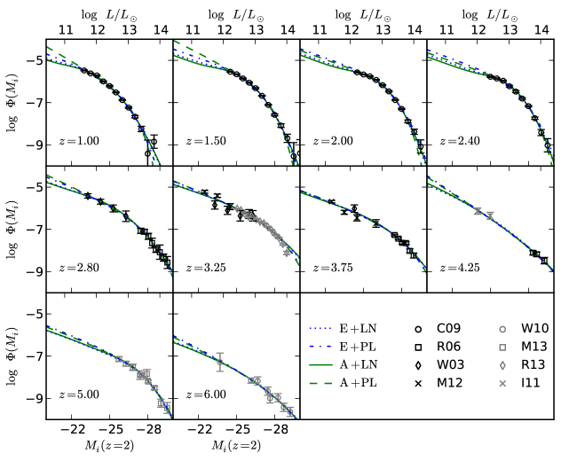
Figure 2: Fit results for each redshift. The lines representing each model variation follow the same abbreviations, colors, and line styles as in figure 1. The data references are as follows: C09 (black circle) is Croom et al. (2009), R06 (black square) is Richards et al. (2006), W03 (black diamond) is Wolf et al. (2003), M12 (black X) is Masters et al. (2012), W10 (gray circle) is Willott et al. (2010), M13 (gray square) is McGreer et al. (2013), R13 (gray diamond) is Ross et al. (2013), I11 (gray X) is Ikeda et al. (2011).

3 Fiducial model variations

3.1 Fitting the QLF

Figure 2 shows the resulting best-fit QLF for each model at each redshift, along with the compiled data. (The figure caption lists references for each of the 8 sources of data.) To compare our model to this data, we use the relation from Shen et al. (2009) between $i$-band magnitude at $z=2$ and bolometric luminosity, in terms of $L_{\odot}$:

$$M_{i}(z=2)=6.04-2.5\log\;(L/L_{\odot})$$ (11)

See e.g. the appendix of Ross et al. (2013) for the filter transformations and k-corrections necessary for expressing all of the data in terms of $M_{i}(z=2).$

It is immediately apparent that all four model variations fit the observed QLF with similar levels of success. In order to disentangle the reasons why four physically distinct models can make such similar predictions, we will make a separate detailed analysis of the bright and faint ends of the QLF. Figure 3 will serve as a useful reference point to these discussions, as it shows qualitatively the substantial freedom our luminosity distributions provide in fitting the observed QLF. The parameters $A$ and $\lambda_{0}$ allow us to adjust the QLF horizontally and vertically, while $\sigma$ and $\beta$ allow separate variation in the bright and faint ends of the QLF. Figure 3 uses the Eddington model at $z=2$ as an example, but the same qualitative features apply at all redshifts and for the accretion model as well.

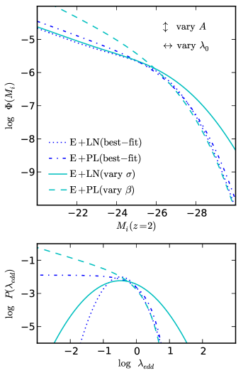
Figure 3: An example of how varying the luminosity distribution $P(\lambda)$ changes the overall QLF. See equations 9 and 10 for the parameterizations of $P_{\rm LN}$ (solid and dotted lines) and $P_{\rm PL}$ (dashed and dash-dotted lines). This shows the best-fit QLF (blue lines) of the Eddington model at $z=2$, and the QLF given by varying $\sigma$ or $\beta$ (cyan lines). For both $P_{\rm LN}$ and $P_{\rm PL}$, varying $A$ simply moves the QLF up or down, and varying $\lambda_{0}$ moves it left or right.

3.2 The bright end of the QLF

We can look back at the second column of figure 1, to see that the “intrinsic” QLF falls off more quickly in the accretion model than in the Eddington model, especially at low redshift. Physically, this is due to the impact of “downsizing” on BH growth rates: while the massive end of the BHMF remains relatively stable, there is a dwindling supply of very quickly growing objects at low redshift, because the more massive objects are already “in place.” However, in spite of this difference in the “intrinsic” QLF, both the Eddington and accretion models have similar success in fitting the QLF at the bright end. This suggests that it is scatter, not the “intrinsic” QLF, that sets the bright end of the observed QLF.

In figure 3, we can see that adjusting $\sigma$ can have a large effect on the bright end of the QLF, whereas adjusting $\beta$ does not. However, the best-fit distributions, shown in blue, are very similar at the large $\lambda$ end for both $P_{\rm LN}$ and $P_{\rm PL}$. This shows that the bright end of the $P(\lambda)$ distribution is well-constrained by the QLF, and that the amount of “scatter” in the luminosity at the exponential cutoff of $P(\lambda)$ is, somewhat coincidentally, approximately the right amount of scatter to fit the QLF. This was illustrated in H14 as well, where most of the discrepancy between the “intrinsic” QLF (in H14, based on the observed galaxy star-formation rate) and the observed QLF could be accounted for by the quasar variability in $P(\lambda)$.

The lack of flexibility in $P_{\rm PL}$ for adjusting the bright end of the QLF does manifest as a slight under-prediction of the bright end of the QLF at certain redshifts. However, our fiducial model neglects scatter in the BH-galaxy relationship: including this additional scatter would likely be enough to resolve this under-prediction in the case of $P_{\rm PL}$, while in the case of $P_{\rm LN}$ it would be easy to decrease $\sigma$ to compensate for increased scatter in the rest of the model. In other words, the bright end of the $P(\lambda)$ is well-constrained by the QLF in our model, but in general it is only the combination of $P(\lambda)$ and scatter in the BH-galaxy relationship that is actually well constrained.

The conclusion that “the bright end of the QLF is set by scatter” is a general one, and regardless of the impact of scatter in the BH-galaxy relationship, this fact allows two physically distinct models to both successfully predict the observed QLF. Even though the Eddington model and the accretion model look quite different at the bright end of the “intrinsic” QLF, quasar variability erases this difference in the observed QLF. The impact of scatter on the properties of very luminous quasars also goes beyond the QLF; for example, scatter can explain why hyperluminous quasars appear to live in halo environments that are very similar to less luminous quasars, as discussed in e.g. Trainor & Steidel (2012), Fanidakis et al. (2013). We will return to the question of how scatter impacts the expected host environments of luminous quasars in section 4.3.

3.3 The faint end of the QLF

The characteristics of the faint end of the QLF are very different from the bright end. Looking again at the second column of figure 1, we can see that the Eddington and accretion models have very similar slopes at the faint end of the “intrinsic” QLF. In contrast, the third column of figure 1 illustrates how different the faint ends of the luminosity distributions are. The fact that models using both $P_{\rm LN}$ and $P_{\rm PL}$ can successfully fit the observed QLF suggests that the faint end of the QLF is set by the “intrinsic” QLF, not by $P(\lambda)$. In other words, the faint end of $P(\lambda)$ is poorly constrained by the observed QLF, which is the opposite of the situation at the bright end of the QLF.

However, the models using $P_{\rm PL}$ do diverge from the models using $P_{\rm LN}$ at low redshift, below the range of the data. This occurs for larger values of $\beta$ (closer to $\beta=1$), and suggests that the faint end of the QLF may depend on quasar variability after all. Such a situation is described in e.g. Hopkins & Hernquist (2009), which contains an extensive discussion of the differences between scattered lightbulb models and luminosity dependent lifetime models.

There are two related reasons for the ambiguity in what governs the slope of the faint end of the QLF. First, there are the limits to our observational data. If we could obtain fainter data, e.g. down to $M_{i}(z=2)=-20$ at $z=1$, we could better distinguish among models. This is complicated, however, by the second problem: the faint-end slope of the QLF may coincidentally be similar to both the slope of the BHMF and to the slope of $P(\lambda)$. (Because the BH growth rate is roughly proportional to its mass, a fact we will return to in sections 3.4 and 4.2, all statements about the BHMF in the Eddington model apply to the accretion model as well.) The faint-end slopes of our “intrinsic” QLFs correspond to roughly $\beta=0.4$ to $0.6$. The slopes of $P_{\rm PL}$ suggested in H14 and Hopkins & Hernquist (2009) are also roughly $\beta=0.4$ and $\beta=0.6$. This make it difficult to distinguish, at the level of the observed QLF, between scattered lightbulb models and luminosity-dependent lifetime models. Fairly precise measurements of the faint-end slopes would be required to detect any difference. (A “pure” lightbulb model with no scatter at all, or a power-law distribution with a hard cutoff at the bright end, might also be able to reproduce the faint end of the QLF; however, they would fail at the bright end, as we discussed in section 3.2.)

Another complication is the following: while a QLF slope that was significantly different from the BHMF slope (thus suggesting that the slope is governed by $P(\lambda)$) would be good evidence for a luminosity-dependent lifetime model, very similar slopes are not necessarily evidence against such a model. Similar slopes in the BHMF and QLF only put constraints on how steep $\beta$ can be, because values near $\beta=0$ yield QLFs nearly indistinguishable from those predicted by scattered lightbulb models.

Finally, it is important to mention that although we are discussing the faint-end slope of the QLF as compared to the low-mass-end slope of the BHMF, our fiducial model relies on a (roughly) linear relationship between the BH and galaxy masses to calculate this slope. In other words, we have implicitly assumed that the low-mass slopes of the BHMF and SMF are the same. (Again, these statements apply to the BH growth rates and SFR as well.) As a result, additional QLF data at the faint end could rule out our fiducial lightbulb models without ruling out all scattered lightbulb models; a direct measurement of the BHMF slope is required to truly make the comparisons discussed above, and to attempt to rule out scattered lightbulb models in general based on the QLF alone.

The result of all this ambiguity is that measurements of the QLF do not necessarily constrain feeding models, quasar triggering mechanisms, or other quasar physics that are encoded primarily in a distribution like $P(\lambda)$. We have shown that for our model, the QLF can provide good constraints on the bright end of this distribution, but not the faint end. In other words, faint quasars may be either high mass BHs at the low end of the $P(\lambda)$ distribution or low mass BHs accreting at or near the Eddington limit, as has been pointed out in other works (e.g. Fanidakis et al., 2012; Ross et al., 2013).

There are several types of measurements useful for complementing the QLF and constraining $P(\lambda)$. One choice is to measure $P(\lambda)$ directly, as done in e.g. Kauffmann & Heckman (2009); Hopkins & Hernquist (2009); Bongiorno et al. (2012); Aird et al. (2012, 2013); Azadi et al. (2014). Numerical simulations, such as in Novak et al. (2011, 2012) and Gabor & Bournaud (2013), can also shed some light on $P(\lambda)$. Another measurement choice is to measure average host property as a function of luminosity, which we discuss in detail in section 4.3. Although we focus on average galaxy SFR in section 4.3, other host properties can be used for a similar analysis such as host halo mass (e.g. Shen et al., 2013, and references therein, or many other measurements of quasar clustering and bias). Each of these approaches generally suggests a “luminosity-dependent lifetime” model rather than a “scattered lightbulb” model.

3.4 Parameter correlations and trends

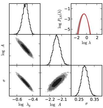
Figure 4: A representative corner plot for the Eddington model convolved with $P_{\rm LN}$ (the “E+LN” model) at $z=2$. The other three model variations (and other redshifts) show qualitatively the same correlations among parameters, replacing $\sigma$ with $-\beta$ where necessary. The red line shows the best-fit $P(\lambda)$ distribution, with the shaded gray region generated from a random sample of points from the MCMC chain, plotted with some transparency. Parameter correlations are shown with 1, 2, and 3-sigma regions (in dark, medium, and light gray).

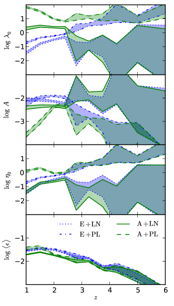
Figure 5: Model parameters vs redshift. The colors and line styles for each of the four model variations again follow the same conventions as in figures 1 and 2. The shaded regions represent the uncertainty in parameters from the MCMC fit.

In figure 4 we show an example of the MCMC fit results, for the Eddington model using a $P_{\rm LN}$ distribution at $z=2$. The general shapes of the parameter correlations are the same for all model variation and redshifts, including models using $P_{\rm PL}$ (when $\sigma$ is replaced by $-\beta$). The best-fit parameters are highly correlated, and we make particular note of the correlation between $\lambda_{0}$ and $A$, which results in a very small error on $\langle\lambda\rangle$. In a very rough approximation, we can write the average $\lambda$ as

$$\log\,\langle\lambda\rangle\sim\log\,A-\log\,\lambda_{0}$$ (12)

which follows the correlation of $A$ and $\lambda_{0}$ in the MCMC fit results. This is notable because, as we see below, the efficiency $\langle\epsilon\rangle$ is related to $\langle\lambda\rangle$. The correlations of both $A$ and $\lambda_{0}$ with $\sigma$ are also fairly strong, but do not directly impact any “physical” parameters of the model. These correlations can be understood by referencing figure 3: increasing $\sigma$ “boosts” the bright end of the QLF, and leaves the faint end unchanged. To “undo” this change and keep a good fit to the data, the QLF must be shifted up and left, by increasing $A$ and decreasing $\lambda_{0}$.

Figure 5 shows the best-fit parameters $\lambda_{0}$ and $A$ as a function of redshift for each model, along with the characteristic Eddington ratio $\eta_{0}$ and average efficiency $\langle\epsilon\rangle$. We can use the the specific growth rate of the BH, $\psi_{\rm BH}\propto\langle\dot{M}_{\rm BH}\rangle/M_{\rm BH}$, to easily calculate $\eta_{0}$ and $\langle\epsilon\rangle$ for all model variations:

$$\eta_{0} =\frac{L_{0}}{L_{edd}}=\lambda_{edd}=\lambda_{acc}\frac{L_{acc}}{L_{edd}}=\frac{\lambda_{acc}}{\psi_{\rm BH}}$$ (13)

$$\langle\epsilon\rangle =\frac{\langle L\rangle}{L_{acc}}=\langle\lambda_{acc}\rangle=\langle\lambda_{edd}\rangle\psi_{\rm BH}$$ (14)

$$\text{where}\;\psi_{\rm BH}\equiv\frac{L_{acc}}{L_{edd}}\propto\frac{\langle\dot{M}_{\rm BH}\rangle}{M_{\rm BH}}$$ (15)

We have defined $\psi_{\rm BH}$ in units convenient to the problem at hand, but it is analogous to the specific star formation rate of galaxies. In reality, $\psi_{\rm BH}$ is a function of BH mass, but over much of the mass range in question it is approximately constant, similar to the specific star formation rate discussed in the appendix. The efficiency we have defined here is closely related to the radiative efficiency; however, radiative efficiency would typically be defined in terms of the total mass inflow, as opposed to the amount of mass ultimately accreted onto the black hole, which in this case would be $\epsilon_{\rm rad}=L/(L+L_{acc})$. For small values of $\epsilon$ the difference between these is small. When we refer to “the efficiency”, we are referring to the definition in equation 14 unless specified otherwise.

There are four notable features of figure 5.

• The uncertainty of the fit parameters increases dramatically starting at redshift $z=2.8$.

• The Eddington models (in blue) and accretion models (in green) give nearly identical predictions for the “physical” parameters, Eddington ratio and efficiency, while the resemblance is not as clear in $\lambda_{0}$ and $A$.

• The uncertainty on the efficiency is much smaller than the uncertainty on the other parameters, and does not increase much with redshift.

• The efficiency is nearly constant at around 3% at $z=1$, but drops gradually with increasing redshift, while the Eddington ratio for the $P_{PL}$ models increases with redshift to greater than 10.

The second item, the similarity between Eddington and accretion models, has already been discussed somewhat in 3.2 and 3.3. The “intrinsic” QLFs in the Eddington and accretion models are very similar at low mass (or low growth rate), where our approximation of constant $\psi_{\rm BH}$ is good. Although they are somewhat different at high mass, this difference is “washed out” by quasar variability when fitting the QLF. We will explore the validity of the constant $\psi_{\rm BH}$ approximation further in section 4.2, but find that it does not have much impact on our analysis.

The first and third items are closely related, having to do with the correlation between $\lambda_{0}$ and $A$. As discussed in section 3.1, $\lambda_{0}$ can adjust the QLF left or right while $A$ can adjust it up or down. Thus, if the observed QLF were a single power-law at all scales, there would be a perfect degeneracy between these two parameters. Instead, the QLF has a “knee”, which limits the degeneracy. However, that “knee” becomes less prominent at high redshift, restoring some of the degeneracy. This is not (necessarily) due to a failure to sample faint luminosities below the “knee” at high redshift, but is due to a combination of larger error bars on the data and a less prominent “knee” inherited from the BHMF and galaxy SMF.

An increased degeneracy between $\lambda_{0}$ and $A$ does not, however, increase uncertainty in $\langle\lambda\rangle\sim\langle\epsilon\rangle$. The efficiency is well constrained at all redshifts, given the assumptions of our model. This illustrates the robustness of classic arguments, such as in Soltan (1982), about the connection between quasar luminosities and BH masses. This argument sets constraints on the radiative efficiency of BHs by comparing the total integrated luminosity of the QLF to the total integrated mass growth of the BHMF. Since all of our fiducial model variations use the same BHMF, output a similar QLF, and assume a single (approximately) mass-independent efficiency, it is unsurprising that the efficiency is very similar across model variations. (Variations beyond our fiducial model, which consider different assumptions about the BHMF, would be expected to give different values for the efficiency.) For any model, correlations in the parameters of our fit may increase the uncertainty of individual parameters such as $A$ and $\lambda_{0}$, but they do not increase the uncertainty of the efficiency because it depends more directly, in some sense, on the final shape of the QLF.

Finally, the fourth item raises several questions about the physical implications of our model(s). Substantially super-Eddington accretion may be physically questionable, and it can be argued that efficiency and Eddington ratio may not be expected to evolve much with redshift (or other parameters) if they are set largely by some universal accretion physics.

The large Eddington ratios for the $P_{\rm PL}$ model variations may be explained by the lack of “adjustable” scatter in those versions of the model. If the bright end of the QLF is set by $P(\lambda)$, as discussed in section 3.2, then $P_{\rm PL}$ has less flexibility in fitting this portion of the QLF, as illustrated in figure 3. Any additional source of scatter would likely decrease the Eddington ratio. (Some examples of additional sources of scatter include modifying $P_{\rm PL}$, adding scatter to the BH-galaxy mass relationship, or accounting galaxy growth beyond what is derived by our simple matching procedure, such as populations of massive galaxies that are still rapidly growing.) This follows the behavior shown in figure 4 for $P_{\rm LN}$, where increasing $\sigma$ correlates with decreasing $\lambda_{0}$ in the MCMC fit.

The best-fit values of Eddington ratio and efficiency also depend on our choice of fiducial model, the “growth-based evolution” model of the BH-galaxy connection. The Eddington ratio is degenerate with $\alpha_{M}$, while the efficiency is degenerate with $\alpha_{G}$. As we discuss in section 4.1 and in the appendix, our fiducial model is only one possible choice. An increase in $\alpha_{M}$ at late redshift could shift the best-fit Eddington ratio down, or a decrease in $\alpha_{G}$ could shift the efficiency up. There is also the issue of obscuration to consider, as the addition of a substantial “obscured fraction” to the calculation would increase the true average efficiency from what is shown in figure 5. We refer to e.g. Gilli et al. (2010) for a discussion of how quasar obscuration may evolve with redshift, but note that it is unlikely for a simple overall obscuration fraction (independent of mass and luminosity but evolving with redshift) to account for nearly two orders of magnitude in evolution of the efficiency. This may imply a “true” decrease in efficiency at high redshift, but we do not make any strong conclusions because of the potential for both obscuration and different choices of $\alpha_{G}$ to modify our result.

4 Beyond the fiducial model

4.1 Choices of redshift evolution

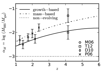
Figure 6: This plot shows $\alpha_{M}$ for each model of the BH-galaxy connection, as a function of redshift, compared to data on the $M_{\rm BH}/M_{\rm gal}$ relation. The data are a compilation from the following sources: M06 (circle) is McLure et al. (2006), T12 (square) is Targett et al. (2012) (with the two points representing two choices for estimating galaxy masses), D10 (diamond) is Decarli et al. (2010), P06 (X) is Peng et al. (2006).

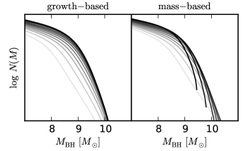
Figure 7: A comparison of the BHMF history for the growth-based evolution model (left panel) and mass-based evolution model (right panel), with the same conventions as the top left panel of figure 1. The darkest lines represent $z=1$, and the lightest gray represent $z=6$. The right panel shows the inconsistency in the BHMF history for the mass-based evolution model, where the high mass end of the BHMF shrinks at low redshift.

Throughout section 3 we have been working within the “growth-based evolution” model of the BH-galaxy relationships across redshift, but that is only one possible model choice. Now we would like to explore the consequences of changing this model, first by considering “mass-based evolution” and “non-evolving” models. We will continue to enforce self-consistency in the BHMF history so that we can make direct comparisons to all four fiducial model variations.

We will also continue to neglect scatter in the BH-galaxy relationships, so the differences in the BH properties of the three models can be expressed entirely by the parameters $\alpha_{M}$ and $\alpha_{G}$, which we defined in section 2.2 as:

$$M_{\rm BH} =10^{\alpha_{M}}M_{\rm gal}$$

$$\langle\dot{M}_{\rm BH}\rangle =10^{\alpha_{G}}\dot{M}_{\rm gal}$$

The appendix derives the behavior of $\alpha_{M}$ and $\alpha_{G}$ for the three models, which we summarize here:

• Growth-based evolution

  $$\alpha_{G}(z) =-3.5+2\log(1+z)$$ (16)

  $$\alpha_{M}(z,M_{\rm gal}) \approx-3.2+2\log(1+z)$$ (17)

• Mass-based evolution

  $$\alpha_{M}(z) =-3.0+2\log(1+z)$$ (18)

  $$\alpha_{G}(z,M_{\rm gal}) \approx-3.3+2\log(1+z)$$ (19)

• Non-evolving

  $$\alpha_{G}=\alpha_{M} =-3.0$$ (20)

The approximate mass-independent versions are more accurate at low mass, and also ignore a slight additional redshift evolution. Figure 6 shows $\alpha_{M}$ for each model compared to a collection of $M_{\rm BH}/M_{\rm gal}$ data. Both evolving models match the data fairly well, but the non-evolving model does not. We also note the difference in our choices for the local values of $\alpha$ in the two models: $\alpha_{G}=-3.5$ and $\alpha_{M}=-3.0$. These are both motivated by observation (e.g. Chen et al. (2013) for $\alpha_{G}$; e.g. Häring & Rix (2004), McConnell & Ma (2013) for $\alpha_{M}$), but seem to have some offset. In Chen et al. (2013), several possible explanations are mentioned for this offset, including substantial obscured accretion activity and a need to account for bulge vs disk vs total galaxy distinctions. However, in our model such an offset occurs naturally as a consequence of evolution in the BH-galaxy relationship. (The value of this offset is approximately 0.3 at $z=1$, but may be greater at $z=0$. Also note that the precise local value of $\alpha_{G}=-3.5$ (or $\alpha_{M}=-3.0$) may be freely tuned to better fit observations with no impact on the overall model properties due to the degeneracy with $\lambda_{0}$.)

Enforcing self-consistency in the BHMF also means that the mass-based evolution model breaks down at low redshift. This was the approach taken in CW13, and the inconsistent BH mass histories were mentioned in that paper. Figure 7 compares the BHMF history of the mass-based model with that of the growth-based model. This figure uses the same convention for redshift as figure 1, with the darkest line corresponding to $z=1$ and the lightest gray corresponding to $z=6$. Here it is easy to see the “shrinking” of the high-mass end of the BHMF in the mass-based evolution model. This failure of self-consistency means that the mass-based evolution model, when coupled with the accretion model for determining the QLF, cannot fit the QLF at all; there is no “intrinsic” QLF to start from, because the accretion rate is negative for nearly all BHs.

In all of our model variations (Eddington vs accretion models using $P_{\rm LN}$ vs $P_{\rm PL}$), the parameter $\lambda_{0}$ is entirely degenerate with either $\alpha_{G}$ (in the accretion models) or $\alpha_{M}$ (in the Eddington models). With the exception of $\alpha_{G}$ in the mass-based model, which is ruled out altogether for low redshift, we can ignore any mass-dependence in $\alpha_{M}$ and $\alpha_{G}$ when discussing this degeneracy. (We will justify this further in section 4.2.) This means that for the purposes of fitting the QLF, the only difference among successful models of the BH-galaxy relationship evolution is a shift in the best-fit value of $\lambda_{0}$, which depends only on redshift and compensates for the shift in $\alpha_{M}$ or $\alpha_{G}$. For example, in the non-evolving model, the best-fit values of Eddington ratio and efficiency would be shifted up from their values in figure 5 by a factor of approximately $2\log(1+z)$.

In summary, there are several potential concerns to consider in choosing a model for the BH-galaxy relationship:

• Ensuring self-consistent $\alpha_{M}$ and $\alpha_{G}$.

• Matching with observations of the $M_{\rm BH}/M_{\rm gal}$ and $\langle\dot{M}_{\rm BH}\rangle/\dot{M}_{\rm gal}$ relations, at each redshift.

• Avoiding substantially super-Eddington accretion or unrealistic efficiency.

• Tuning the model to obtain Eddington ratios or efficiencies that do (or do not) evolve with redshift in some desired way.

Our fiducial model succeeds with the first three concerns listed, while tuning the model to keep either Eddington ratio or efficiency constant in redshift would require a more thorough exploration of the “model space” for $\alpha_{G}$ and $\alpha_{M}$ than our three example choices. We note that keeping both Eddington ratio and efficiency constant within this framework may not be possible, since $\alpha_{M}$ and $\alpha_{G}$ cannot be tuned independently.

While a general trend of increasing $\alpha$ at increasing redshift is helpful both in matching the observed $M_{\rm BH}/M_{\rm gal}$ data and in avoiding concerns about super-Eddington accretion and high efficiency, it does present a potential challenge for BH seeding models. We will not discuss this issue further, but it is an important one to consider for connecting the model to redshifts beyond $z=6$.

4.2 High mass objects and “downsizing”

We return to the growth-based evolution model to discuss the impact of “downsizing” on specific growth rates and related model assumptions. At several points throughout the paper, we have used the approximation that the specific growth rate of both galaxies ($\psi$ in the appendix) and black holes ($\psi_{\rm BH}$) is independent of mass. This then allows us to assume that $\alpha_{G}$ and $\alpha_{M}$ are both independent of mass as well, and results in the simple conversion between Eddington ratio and efficiency in section 3.4.

However, a mass-independent $\alpha_{M}$ and $\psi_{\rm BH}$ are unlikely to be the case. In our model, $\psi_{\rm BH}$ is roughly independent of mass at the low-mass end, but drops off at high mass, eventually dropping sharply to zero for objects that are no longer growing at all. The mass scale at which this occurs gets smaller at smaller redshift, meaning the impact of this “downsizing” is largest at small redshifts.

At high mass, where $\psi_{\rm BH}=0$, the parameter conversions from section 3.4 give zero for the Eddington ratio in the accretion models, and infinity for the efficiency in the Eddington models. Infinite radiative efficiency is clearly not physically reasonable, so we adjust the Eddington model to “turn off” these high mass BHs. This is done by simply truncating the BHMF to include only objects with a nonzero growth rate before we use it to derive the “intrinsic” QLF. The impact of this adjustment on the observed QLF is completely negligible; the Eddington models fit the QLF equally well, with the same parameters, whether we truncate the BHMF or not. If we go a step further and truncate the BHMF to exclude masses where the growth rate is no longer increasing with mass (which represents the mass scale at which the specific growth rate begins to drop rapidly towards zero), the effect on the QLF is still negligible, and is only detectable at all at very low redshift and very high luminosity.

Physically, the difference between the Eddington and accretion models is most relevant in a limited range of masses, where we find objects in “transition”: their growth is slower than the characteristic specific growth rate at that redshift, but has not stopped completely. The Eddington model assumes these objects shine with the same distribution of Eddington ratios as “normal” objects, which would require a larger radiative efficiency. The accretion model assumes these objects have the same distribution of $\lambda_{acc}$, and hence the same average efficiency, as “normal” objects, which results in a lower Eddington ratio. In principle, a hybrid model is also possible, which holds both Eddington ratio and average efficiency fixed, but instead adjusts the duty cycle (the normalization of the $P(\lambda)$ distribution) for these “transition” objects to keep everything self-consistent. It is virtually impossible, however, to tell the difference between models at the level of the QLF, because of the effects mentioned in section 3.2. Subtle effects such as this at the high mass end are entirely “washed out” by the scatter contained in the luminosity distributions $P(\lambda)$. (This scatter is also what allows us to “turn off” the zero-growth BHs entirely in the Eddington model without impacting the QLF.) In other words, for the purposes of fitting the observed QLF the Eddington and accretion models are essentially equivalent.

Another effect of a mass-dependent $\psi_{\rm BH}$ (and thus $\alpha_{M}$) is curvature in the $M_{\rm BH}/M_{\rm gal}$ relationship. This effect is also relevant only at high mass and low redshift. Even at $z\approx 1$, we find only a factor of 2 increase in $M_{\rm BH}$ at the largest mass scales, compared to the linear $M_{\rm BH}/M_{\rm gal}$ relation. This is easily consistent with the current uncertainty in observational measurements of the local BHMF (e.g. McConnell & Ma (2013)).

4.3 Quasar host properties and BH-galaxy scatter

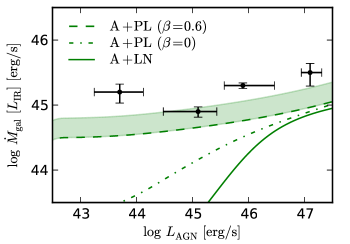
Figure 8: Average galaxy SFR (expressed in terms of $L_{\rm IR}$) in bins of quasar luminosity. All lines shown are for the fiducial (growth-based evolution) accretion model at $z=2$. The solid line shows the model with $P_{\rm LN}$. The dash-dotted line shows the model with a flat slope in $P_{\rm PL}$. The dashed line shows the model with a steep slope in $P_{\rm PL}$. Because we use the total mass growth rate as an approximation to the SFR, neglecting stellar mass loss and other effects, we expect all of these lines to represent a low estimate of the true SFR. The dashed green line (our “best-fit” model in this case) is shown with a shaded region representing the expected correction (up to a factor of 2) to our calculation. The data points are from Rosario et al. (2012), and show the observed $L_{\rm IR}$ for the redshift bin $1.5<z<2.5$.

There are many observables beyond the QLF that can be used to investigate models of quasar demographics. We refer to H14 for a detailed discussion of the important distinction between measuring average quasar luminosity in bins of host property versus measuring average host property in bins of quasar luminosity. We have constructed a similar model here: by design, average quasar luminosity has a simple linear correlation with either galaxy mass or growth rate. The inverse calculation, on the other hand, is very sensitive to the various sources of scatter in the model.

Figure 8 shows the average host galaxy “SFR” as a function of quasar luminosity, for three variations of our fiducial (growth-based evolution) accretion model. We write “SFR” in quotation marks because we have only calculated an approximation to the real galaxy SFR; in addition to the crudeness of our constant-number-density matching procedure, we are neglecting factors such as stellar mass loss. Our “best-fit” model in this case is the variation with $P_{\rm PL}$ and a steep $\beta$: we show it with a shaded band representing the region between our approximate SFR, which is likely to be a low estimate, and the “true” SFR which may be larger by a factor of 2 or more. (See e.g. Behroozi et al. (2013).) Our results are similar to those in figure 3(b) of H14, except that we show a weaker correlation at the high luminosity end. Although we show only $z=2$ in figure 8, we do reproduce the trend in H14 that the “characteristic” SFR of low-luminosity quasars decreases with decreasing redshift. However, the trend reverses above about $z=3$ and begins to decrease with increasing redshift, meaning the characteristic SFR for low-luminosity quasars has a peak around $2<z<3$.

Unlike the QLF, the measurement in figure 8 is quite sensitive to the difference between models using $P_{\rm LN}$ and those using $P_{\rm PL}$, and to the slope $\beta$ of $P_{\rm PL}$. The weak correlation of SFR and quasar luminosity (for low-luminosity quasars) is good evidence for a $P(\lambda)$ that not only resembles $P_{\rm PL}$, but has a fairly steep power-law $\beta$. The correlation at high luminosity, on the other hand, is very similar for all of the models, because of how well-constrained the bright end of $P(\lambda)$ is by the QLF. However, $P(\lambda)$ itself is only well-constrained because of our decision to neglect scatter in all of our other model relationships. For measurements such as the one illustrated in figure 8, the degeneracy between different sources of scatter (between BH and galaxy properties, in $P(\lambda)$, between galaxy mass and SFR, etc.) becomes important. For example, we could imagine that there is substantial scatter between galaxy mass and SFR, which would substantially boost the bright end of the “intrinsic” QLF in the accretion models. To compensate for this, and keep a good fit to the observed QLF, we would have to decrease the amount of “scatter” in the bright end of $P(\lambda)$, by making the exponential cutoff sharper somehow or decreasing $\sigma$ for $P_{\rm LN}$. This would result in a substantially stronger correlation at high luminosity in figure 8, because there would be less scatter (at the bright end) between the SFR and QLF.

We can imagine our model, for the growth-based evolution and accretion model case, as the following chain of calculations: halo mass $\rightarrow$ galaxy mass $\rightarrow$ galaxy SFR $\rightarrow$ average BH accretion rate $\rightarrow$ BH “intrinsic” luminosity $\rightarrow$ observed quasar luminosity. At each step there is potentially some amount of scatter in the relations governing our calculation, although we have neglected all sources of scatter outside $P(\lambda)$ and the galaxy-halo mass relations. Since the total amount of scatter (at the high mass/luminosity end, for a known halo mass function) is well constrained by the QLF, we can only “redistribute” this scatter among the steps listed. If we imagine making a measurement similar to figure 8 for each of the host properties, the correlation at high luminosity will depend on the amount of scatter between that particular property and the end of our “chain” of calculations. Thus, we expect the correlation between host halo mass and quasar luminosity to be very weak regardless of our other decisions about scatter. This is roughly equivalent to saying that we do not expect the most luminous quasars to live in halo environments very different from those of less luminous quasars, which in turn impacts the luminosity dependence of quasar bias and clustering (e.g. Trainor & Steidel (2012), Fanidakis et al. (2013) as mentioned in section 3.2). On the other hand, the correlation between average BH accretion rate (or mass, if we were to do this procedure for the Eddington models) and quasar luminosity could be quite strong. This is roughly the situation described in e.g. Hopkins & Hernquist (2009), where very luminous quasars are typically objects accreting at (or near) the Eddington luminosity. Again, this only applies to the correlation for very luminous quasars; if the models with $P_{\rm PL}$ and steep $\beta$ are correct, then the very weak correlations at low luminosity would be expected for any host property calculated as in figure 8.

5 Summary

We have constructed a self-consistent model of quasar demographics, which links BH growth to galaxy growth across redshift and derives BH masses by integrating this growth history. This model has four variations wtihin the fiducial model: “intrinsic” quasar luminosities are tied to either BH mass (the “Eddington model”) or BH growth rate (the “accretion model”), and quasar variability is modeled by either a “scattered lightbulb” model (a lognormal luminosity distribution) or a “luminosity-dependent lifetime” model (a power-law distribution with arbitrary lower bound and exponential cutoff), shown schematically in figure 1.

All four variations successfully fit the observed QLF (shown in figure 2), despite being physically distinct models. The “Eddington” and “accretion” models are made nearly impossible to distinguish by the similarity in their “intrinsic” QLFs at low luminosity, which stems from the very weak dependence of specific growth rates on mass (for both BHs and galaxies), and the fact that the “intrinsic” QLF derived from the BHMF may be truncated to include only objects with nonzero growth without impacting the fit to the QLF. The remaining differences at high luminosity are washed out by scatter, so that both models can fit the bright end of the QLF despite differences in the bright ends of the “intrinsic” QLFs, and regardless of whether the largest (non-growing) objects in the BHMF are included.

The “scattered lightbulb” and “luminosity-dependent lifetime” models are difficult to distinguish because they are extremely similar at the bright end of the luminosity distribution, which is relatively well constrained by the QLF. Their main difference is in the faint end of the distribution, which is very poorly constrained by the QLF. However, measurements of the correlations between quasar luminosity and host property (galaxy mass, SFR, BH mass, etc.) are more sensitive to the details of various sources of scatter than the QLF. Our model predicts, by design, a straightforward linear correlation when measuring average quasar luminosity in bins of host property. The inverse measurement, of average host property in bins of quasar luminosity, is much more sensitive to scatter, with increased scatter resulting in a weaker correlation. Weak correlations at low luminosity are good evidence for “luminosity-dependent lifetime” models, with weaker correlations implying steeper power-law slopes. At high luminosity, the strength of the correlation can potentially be used to distinguish between different sources of scatter, such as scatter in the BH-galaxy relationship (which we have neglected) vs scatter in $P(\lambda)$.

Individual parameters in our model, particularly the characteristic Eddington ratio and normalization of the luminosity distribution, have increasing degeneracy at high redshift due to the “softening” of the “knee” of the QLF. The average efficiency, on the other hand, is comparatively well-constrained at all redshifts and has very similar best-fit values for all four model variations. While the instantaneous efficiency may still be some strong function of luminosity in our model, the average efficiency is well constrained by the oberved QLF and BHMF alone.

Finally, requiring self-consistent redshift evolution in the BH-galaxy relationship gives important constraints on the degeneracies in the model. Based on fitting the QLF alone, there is a perfect degeneracy between e.g. the normalization of $M_{\rm BH}/M_{\rm gal}$ ($\alpha_{M}$) and the characteristic Eddington ratio ($\lambda_{0}$ in the Eddington model). However, figure 6 illustrates the need for some form of redshift evolution in $\alpha_{M}$ to match the observed $M_{\rm BH}/M_{\rm gal}$ evolution. As discussed in the appendix, it is impossible to keep a strictly linear relationship in both $M_{\rm BH}/M_{\rm gal}$ and $\langle\dot{M}_{\rm BH}\rangle/\dot{M}_{\rm gal}$ while including redshift evolution, so our fiducial “growth-based” model implies some curvature in $M_{\rm BH}/M_{\rm gal}$. A “mass-based” model, on the other hand, results in an inconsistent BHMF history (illustrated in 7), so we can rule it out within our model framework. The curvature we predict in $M_{\rm BH}/M_{\rm gal}$ is slight, restricted to high mass, and increases with decreasing redshift.

A general conclusion of our model is that there are substantial degeneracies within the “model space” of simple quasar demographics models. We’ve explored three types of observation that are in some sense “orthogonal” and helful to breaking these model degeneracies:

• The QLF can be fit equally well by many models, and is a well-studied output of large-scale redshift surveys, so it serves as an input to the model, fixing the best-fit model parameters (within certain degeneracies) which can then be used to “predict” other observables.

• The $M_{\rm BH}/M_{\rm gal}$ relation allowed us to fix a “fiducial model” of the BH-galaxy relationship, which would otherwise be quite unconstrained due to degeneracies between $\alpha_{M}$ (or $\alpha_{G}$) and $\lambda_{0}$. Making the connection across redshifts to require a self-consistent BHMF history further refines this model by ruling out our mass-based evolution in favor of growth-based evolution.

• Measurements of average host property in bins of quasar luminosity are much more sensitive to the various sources of scatter in the model than the QLF. Weak correlations at the low luminosity end are evidence for models wherein quasars spend a large amount of time at relatively low luminosity, while comparing the correlations at high luminosity of different host properties may help identify which sources of scatter are most relevant to very luminous quasars.

The most persistent “degeneracy” in our model is between our “Eddington” and “accretion” models. To some degree, this represents a true physical equivalence in our overall model, because the BH mass and growth rate are roughly proportional to each other over much of the relevant mass range. At very high mass, however, “downsizing” results in massive objects that are no longer growing, which would imply infinite radiative efficiency in the simplest version of the Eddington model. We showed that adjusting the Eddington model to “turn off” those high mass objects has no impact on our model predictions, except for small effects at our lowest redshifts. A more sophisticated method of connecting BHs and galaxies across redshifts could extend our model to lower redshift, where the difference between Eddington and accretion models may no longer be negligible.

To extend the model to $z<1$, following the methods of Behroozi et al. (2013) in more detail (e.g. by following halo merger trees instead of matching galaxies at constant number density on the SMF) is one possible way to obtain the necessary self-consistent galaxy histories in that redshift range. More generally, any method that connects galaxies across redshifts in a self-consistent way, tracking both mass and growth rates, would be suitable for our model framework. Breaking the various “degeneracies” in our model illustrates the value of a diverse data set spanning multiple redshifts, luminosity ranges, and measurable quantities, such as can be provided by large-scale redshift surveys.

Appendix A Redshift evolution

Our fiducial model, as well as the variations we consider in section 4, enforces self-consistent BHMF growth across redshifts by associating objects at constant number density. We define two parameters, $\alpha_{M}$ and $\alpha_{G}$, which encode the BH-galaxy relationship, noting that in general they are not the same, and can contain both redshift and mass dependence.

$$M_{\rm BH} =10^{\alpha_{M}}M_{\rm gal}$$ (21)

$$\langle\dot{M}_{\rm BH}\rangle =10^{\alpha_{G}}\dot{M}_{\rm gal}$$ (22)

$$\text{where }\alpha_{M}(z,M_{\rm gal}) \neq\alpha_{G}(z,M_{\rm gal})$$ (23)

The simplest model to consider is the “non-evolving” model, where the $M_{\rm BH}/M_{\rm gal}$ relationship does not evolve with redshift and is a simple linear relationship.

$$\alpha_{M}=\alpha_{G}=\alpha_{0}$$ (24)

The non-evolving model we consider in the main text takes $\alpha_{0}=-3.0$. (We will use $\alpha_{0}$ throughout the appendix to note a constant value, with no mass or redshift dependence.)

Another choice is the model from CW13, which adds a simple redshift evolution to $\alpha_{M}$. We call this the “mass-based evolution” model, and again use $\alpha_{0}=-3.0$ for the example in the main text of the paper. The $(1+z)^{2}$ scaling, used here and in CW13, is chosen as a possible broad match to observational data (as shown in figure 6).

$$M_{\rm BH} =10^{\alpha_{0}}M_{\rm gal}(1+z)^{2}$$ (25)

$$=10^{\alpha_{M}}M_{\rm gal}$$ (26)

$$\implies\alpha_{M} =\alpha_{0}+2\log(1+z)=\alpha_{M}(z)$$ (27)

With this choice of redshift evolution for $\alpha_{M}$, we can then derive $\alpha_{G}$ by taking the time derivative of equation 26 :

$$\langle\dot{M}_{\rm BH}\rangle =10^{\alpha_{M}}\dot{M}_{\rm gal}\left(1+(\ln 10)\dot{\alpha}_{M}\frac{M_{\rm gal}}{\dot{M}_{\rm gal}}\right)$$ (28)

$$=10^{\alpha_{G}}\dot{M}_{\rm gal}$$ (29)

$$\implies\alpha_{G} =\alpha_{M}+\log\left(1+(\ln 10)\dot{\alpha}_{M}\frac{M_{\rm gal}}{\dot{M}_{\rm gal}}\right)$$ (30)

$$=\alpha_{G}(z,M_{\rm gal})$$ (31)

Here we can see that $\alpha_{G}$ must depend on both redshift and mass, since the specific growth rate $\psi\equiv\dot{M}_{\rm gal}/M_{\rm gal}$ depends on mass. This mass dependence is stronger at high mass, so we can find an approximation to $\alpha_{G}$ for small mass where $\psi$ is roughly constant. In the following, we will use equation 27 to evaluate $\dot{\alpha}_{M}$.

$$\alpha_{G} =\alpha_{M}+\log\left(1+(\ln 10)\frac{\dot{\alpha}_{M}}{\psi}\right)$$ (32)

$$=\alpha_{M}+\log\left(1+\frac{2}{1+z}\frac{\dot{z}}{\psi}\right)$$ (33)

$$=\alpha_{M}+\log\left(1-\frac{2H_{0}}{\psi}\sqrt{\Omega_{m}(1+z)^{3}+\Omega_{\Lambda}}\right)$$ (34)

$$\approx\alpha_{M}-0.3$$ (35)

Where the $-0.3$ offset from $\alpha_{M}$ is a very rough approximation, and neglects both the mass dependence and the additional redshift dependence (beyond the redshift dependence of $\alpha_{M}(z)$). For our analysis, we find $\alpha_{G}$ numerically by applying $\alpha_{M}$ to the SMFs, then subtracting across redshifts.

Our fiducial model involves giving a simple redshift evolution to $\alpha_{G}$, then integrating the masses across redshift to obtain $\alpha_{M}$. We call this the “growth-based evolution” model. The same general reasoning applies to this model as to the “mass-based evolution” model, with $\alpha_{G}$ and $\alpha_{M}$ switching roles. The end result is:

$$\langle\dot{M}_{\rm BH}\rangle =10^{\alpha_{0}}\dot{M}_{\rm gal}(1+z)^{2}$$ (36)

$$\implies\alpha_{G} =\alpha_{0}+2\log(1+z)=\alpha_{G}(z)$$ (37)

$$\implies\alpha_{M} =\alpha_{M}(z,M_{\rm gal})$$ (38)

$$\approx\alpha_{G}(z)+0.3$$ (39)

In the text, we use the growth-based evolution model with $\alpha_{0}=-3.5$ as our fiducial model.

References

- Aird et al. (2012) Aird, J., Coil, A. L., Moustakas, J., et al. 2012, ApJ, 746, 90
- Aird et al. (2013) Aird, J., Coil, A. L., Moustakas, J., et al. 2013, ApJ, 775, 41
- Alexander & Hickox (2012) Alexander, D. M., & Hickox, R. C. 2012, New Astronomy Reviews, 56, 93
- Azadi et al. (2014) Azadi, M., Aird, J., Coil, A., et al. 2014, arXiv:1407.1975
- Behroozi et al. (2013) Behroozi, P. S., Wechsler, R. H., & Conroy, C. 2013, ApJ, 770, 57
- Bongiorno et al. (2012) Bongiorno, A., Merloni, A., Brusa, M., et al. 2012, MNRAS, 427, 3103
- Booth & Schaye (2010) Booth C.M., Schaye J., 2010, MNRAS, 405, L1
- Carlberg (1990) Carlberg R.G., 1990, ApJ, 350, 505
- Chabrier (2003) Chabrier, G. 2003, PASP, 115, 763
- Chen et al. (2013) Chen, C.-T. J., Hickox, R. C., Alberts, S., et al. 2013, ApJ, 773, 3
- Conroy & White (2013) Conroy, C., & White, M. 2013, ApJ, 762, 70
- Croom et al. (2009) Croom, S. M., Richards, G. T., Shanks, T., et al. 2009, MNRAS, 399, 1755
- Croton (2009) Croton D.J., 2009, MNRAS, 394, 1109
- Decarli et al. (2010) Decarli, R., Falomo, R., Treves, A., et al. 2010, MNRAS, 402, 2453
- Efstathiou & Rees (1988) Efstathiou G., Rees M.J., 1988, MNRAS 230, 5
- Fanidakis et al. (2012) Fanidakis, N., Baugh, C. M., Benson, A. J., et al. 2012, MNRAS, 419, 2797
- Fanidakis et al. (2013) Fanidakis, N., Macciò, A. V., Baugh, C. M., Lacey, C. G., & Frenk, C. S. 2013, MNRAS, 436, 315
- Gabor & Bournaud (2013) Gabor, J. M., & Bournaud, F. 2013, MNRAS, 434, 606
- Gilli et al. (2010) Gilli, R., Comastri, A., Vignali, C., Ranalli, P., & Iwasawa, K. 2010, X-ray Astronomy 2009; Present Status, Multi-Wavelength Approach and Future Perspectives, 1248, 359
- Haiman, Ciotti & Ostriker (2004) Haiman Z., Ciotti L., Ostriker J.P., 2004, ApJ, 606, 763
- Häring & Rix (2004) Häring, N., & Rix, H.-W. 2004, ApJ, 604, L89
- Hickox et al. (2014) Hickox, R. C., Mullaney, J. R., Alexander, D. M., et al. 2014, ApJ, 782, 9
- Hopkins & Hernquist (2009) Hopkins, P. F., & Hernquist, L. 2009, ApJ, 698, 1550
- Ikeda et al. (2011) Ikeda, H., Nagao, T., Matsuoka, K., et al. 2011, ApJ, 728, L25
- Kauffmann & Heckman (2009) Kauffmann, G., & Heckman, T. M. 2009, MNRAS, 397, 135
- Kormendy & Ho (2013) Kormendy, J., & Ho, L. C. 2013, ARA&A, 51, 511
- Lidz et al. (2006) Lidz, A., Hopkins, P. F., Cox, T. J., Hernquist, L., & Robertson, B. 2006, ApJ, 641, 41
- Marulli et al. (2006) Marulli F., Crociani D., Volonteri M., Branchini E., Moscardini L., 2006, MNRAS, 368, 1269
- Masters et al. (2012) Masters, D., Capak, P., Salvato, M., et al. 2012, ApJ, 755, 169
- McConnell & Ma (2013) McConnell, N. J., & Ma, C.-P. 2013, ApJ, 764, 184
- McGreer et al. (2013) McGreer, I. D., Jiang, L., Fan, X., et al. 2013, ApJ, 768, 105
- McLure et al. (2006) McLure, R. J., Jarvis, M. J., Targett, T. A., Dunlop, J. S., & Best, P. N. 2006, MNRAS, 368, 1395
- Mullaney et al. (2012) Mullaney, J. R., Daddi, E., Béthermin, M., et al. 2012, ApJ, 753, L30
- Novak et al. (2011) Novak, G. S., Ostriker, J. P., & Ciotti, L. 2011, ApJ, 737, 26
- Novak et al. (2012) Novak, G. S., Ostriker, J. P., & Ciotti, L. 2012, MNRAS, 427, 2734
- Peng et al. (2006) Peng, C. Y., Impey, C. D., Rix, H.-W., et al. 2006, NewAR, 50, 689
- Rafferty et al. (2011) Rafferty, D. A., Brandt, W. N., Alexander, D. M., et al. 2011, ApJ, 742, 3
- Richards et al. (2006) Richards, G. T., Strauss, M. A., Fan, X., et al. 2006, AJ, 131, 2766
- Rosario et al. (2012) Rosario, D. J., Santini, P., Lutz, D., et al. 2012, A&A, 545, A45
- Ross et al. (2013) Ross, N. P., McGreer, I. D., White, M., et al. 2013, ApJ, 773, 14
- Shen (2009) Shen Y., 2009, ApJ, 704, 89
- Shen et al. (2009) Shen, Y., Strauss, M. A., Ross, N. P., et al. 2009, ApJ, 697, 1656
- Shen et al. (2013) Shen, Y., McBride, C. K., White, M., et al. 2013, ApJ, 778, 98
- Soltan (1982) Soltan, A. 1982, MNRAS, 200, 115
- Targett et al. (2012) Targett, T. A., Dunlop, J. S., & McLure, R. J. 2012, MNRAS, 420, 3621
- Tinker et al. (2008) Tinker, J., Kravtsov, A. V., Klypin, A., et al. 2008, ApJ, 688, 709
- Tinker et al. (2010) Tinker, J. L., Robertson, B. E., Kravtsov, A. V., et al. 2010, ApJ, 724, 878
- Trainor & Steidel (2012) Trainor, R. F., & Steidel, C. C. 2012, ApJ, 752, 39
- Willott et al. (2010) Willott, C. J., Delorme, P., Reylé, C., et al. 2010, AJ, 139, 906
- Wolf et al. (2003) Wolf, C., Wisotzki, L., Borch, A., et al. 2003, A&A, 408, 499
- Wyithe & Loeb (2002) Wyithe J.S.B., Loeb A., 2002, ApJ, 581, 886
- Wyithe & Loeb (2003) Wyithe J.S.B., Loeb A., 2003, ApJ, 595, 614