Unveiling the near-infrared structure of the massive-young stellar object NGC 3603 IRS 9A* with sparse aperture masking and spectroastrometry

Abstract

Context. Contemporary theory holds that massive stars gather mass during their initial phases via accreting disk-like structures. However, conclusive evidence for disks has remained elusive for most massive young objects. This is mainly due to significant observational challenges: objects are rare and located at great distances within dusty, highly opaque environments. Incisive studies, even targeting individual objects, are therefore relevant to the progression of the field. NGC 3603 IRS 9A* is a young massive stellar object that is still surrounded by an envelope of molecular gas for which previous mid-infrared observations with long-baseline interferometry have provided evidence of a plausible disk of 50 mas diameter at its core.

Aims. This work aims at a comprehensive study of the physics and morphology of IRS 9A at near-infrared wavelengths.

Methods. New sparse aperture-masking interferometry data, taken with the near-infrared camera NACO of the Very Large Telescope (VLT) at $K_{s}$ and $L^{\prime}$ wavelengths, were analyzed together with archival high-resolution H₂ and Br$\gamma$ lines obtained with the cryogenic high-resolution infrared schelle spectrograph (CRIRES).

Results. The trends in the calibrated visibilities at $K_{s}$ and $L^{\prime}$ bands suggest the presence of a partially resolved compact object with an angular size of $\leq$30 mas at the core of IRS 9A, together with the presence of over-resolved flux. The spectroastrometric signal of the $H_{2}$ line, obtained from the CRIRES spectra, shows that this spectral feature proceeds from the large-scale extended emission ($\sim$ 300 mas), while the Br$\gamma$ line appears to be formed at the core of the object ($\sim$ 20 mas). To better understand the physics that drive IRS 9A, we have performed continuum radiative transfer modeling. Our best model supports the existence of a compact disk with an angular diameter of 20 mas, together with an outer envelope of 1” exhibiting a polar cavity with an opening angle of $\sim$30^∘. This model reproduces the MIR morphology that has previously been derived in the literature and also matches the spectral energy distribution of the source.

Conclusions. Our observations and modeling of IRS 9A support the presence of a disk at the core, surrounded by an envelope. This scenario is consistent with the brightness distribution of the source for near- and mid-infrared wavelengths at various spatial scales. However, our model suffers from remaining inconsistencies between SED modelling and the interferometric data. Moreover, the Br$\gamma$ spectroastrometric signal indicates that the core of IRS 9A exhibits some form of complexity such as asymmetries in the disk. Future high-resolution observations are required to confirm the disk/envelope model and to flesh out the details of the physical form of the inner regions of IRS 9A.

1 Introduction

Massive stars play an important role in the evolution of galaxies. They exert a tremendous influence on their surroundings through the mass flows that are produced by their strong stellar winds and by their deaths in the form of supernova explosions. However, in spite of their importance, our knowledge about their births and evolution is still not conclusive. This is mainly because their evolutionary time-scale is of the order of a few Ma. They are formed in dense molecular clouds, that are highly opaque and, by the time they reach the zero-age main sequence, they are still embedded in their parental cloud (Churchwell 2002). Hence, the observation of their initial evolutionary phases is challenging. Furthermore, they are scarce and usually born in dense clusters that are located at large distances ($\geq$ 1 kpc), thus the use of high-angular resolution techniques is required to study them (see the review of Zinnecker & Yorke 2007).

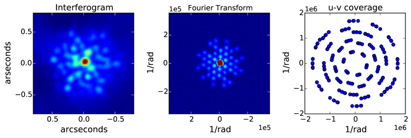
Figure 1: Left: IRS 9A: Average interferogram in the image plane observed in a sparse aperture masking (SAM) data cube. Center: Fourier transform of an average interferogram. The 42 blue spots correspond to the sampled visibilities and their complex conjugates, while the central red spot is the DC component of the Fourier transform and it is proportional to the squared of the total flux in the interferogram. Right: UV coverage of our SAM observations.

There are two contemporary models that seek to explain high-mass star formation: core collapse and competitive accretion. Although both models predict the existence of accretion disks in massive young stellar objects (MYSOs), there are still important questions about the physics of these structures (e.g., sizes, accretion rates, densities, ages). This is mainly because of the lack of observational evidence of such disks owing to the high extinction that affects MYSOs and the necessity of high-angular resolution at infrared wavelengths. One of the most important questions is the role of radiation pressure from luminous central stars (L$\sim$10⁴-10⁵L_⊙) on the physics of the accretion disks. Massive stars have short Kelvin-Helmholtz ($\sim$ 10⁴-10⁵ years) scales, compared to their accretion time-scale. Therefore, by the time the central star is fusing hydrogen, it is still accreting material. Onset of fusion and its increase of a star’s effective temperature lead to a significant increase of overall radiative output and UV radiation, which poses strong constraints on how high-mass stars can accrete matter. For example, Bondi-Hoyle accretion simulations predict that radiation pressure could stop accretion for massive stars $\geq$ 10M_⊙ (Edgar & Clarke 2004). These results highlight the necessity to have protostellar disks to shield the accreting material from the radiation pressure to form the most massive stars.

During the last decade, significant progress has been made, not only in the study of massive protostellar disks, but also of the whole morphology of MYSOs. From the theoretical point of view, many studies have been conducted to explain the different properties of disks in MYSOs, most of them in the context of core collapse. For example, Vaidya et al. (2009) performed steady state models of thin disks around MYSOs to investigate the role of accretion. Additionally, Krumholz et al. (2009) performed 3D simulations of forming massive stars showing the presence of rotational structures (i.e. accretion disks) with high accretion rates ($\sim$10^-4M_⊙/yr). These simulations also support evidence that gravitational and Rayleigh-Taylor instabilities in the disk-like structures overcome the radiation pressure of the star and lead to the formation of companions (but see a different view in Kuiper et al. 2012). Seifried et al. (2011, 2012) present hydrodynamical simulations of collapsing massive cores to explain the role of magnetic fields on the stability of massive disks, concluding that magnetic pressure actively contributes to their stability. On the other hand, Kuiper et al. (2014) determine, through hydrodynamical simulations, that the accretion time of the disk is strongly correlated with the time at which protostellar outflows are present.

Alternatively, significant observational progress was triggered by the advent of adaptive optics (AO) at 8-10m class telescope, infrared interferometry, as well as by the improved sensitivity and angular resolution of millimeter interferometers. For example, radio interferometric observations have found evidence of molecular outflows and jets launched at the core of the MYSOs (e.g., Beuther et al. 2002; Beuther & Shepherd 2005), as well as evidence of disk-like structures that are perpendicular to such outflows (e.g., Beltrán et al. 2005), thus providing us with a picture consistent with the predicted circumstellar disks. Recently, Boley et al. (2013) performed a survey of disks around a sample of 24 intermediate and high-mass stellar objects at MIR wavelengths with MIDI at the Very Large Telescope Interferometer (VLTI). Almost all the observed massive stars of their sample presented elongated structures at scales $\leq$100 AU, which could be associated with disks and/or outflows. Additional MIR interferometry case studies on individual objects include: M8E-IR (Linz et al. 2009), M17 SW IRS1 (Follert et al. 2010), AFGL 4176 (Boley et al. 2012), CRL 2136 (de Wit et al. 2011), and NGC 2264 IRS 1* (Grellmann et al. 2011). We also note that the work of de Wit et al. (2007) was one of the first attempts to perform simultaneous model-fitting to the spectral energy distribution (SED) and mid-infrared interferometric visibilities of W33A. At near-infrared wavelengths, perhaps the most representative case study of disks in MYSOs was performed by Kraus et al. (2010). These authors resolved a hot, compact disk around the MYSO IRAS 13481-6124 (M$\sim$20 M_⊙), carrying out interferometric observations with AMBER/VLTI. The observed structure exhibits a projected elongated shape of 13x19 AU with a dust-free inner gap of 9.5 AU, matching the expected location of the dust sublimation radius for this object.

Apart from the mentioned examples of observing (or modeling) the morphology of MYSOs directly, there have been several studies to characterize MYSOs from their spectra. Two methods are worth mentioning: (i) the characterization of their SED, and (ii) the analysis of the flux centroid of absorption or emission lines through spectroastrometry. An example of the first method is the work of Robitaille et al. (2006). These authors computed a grid of $\sim$10⁵ SED models of YSOs up to masses of 50M_⊙. These models, based on the prescription of Whitney et al. (2003), include the presence of disks, envelopes, and cavities to reproduce observed SEDs. Offner et al. (2012) performed a study to explore the reliability of SED-fitting to obtain physical parameters of low-mass YSOs. They find that solely SED-fitting is not enough to fully characterize the morphology of low-mass YSOs. This is also expected to be true in the high-mass case. Combining spectroastrometry with CRIRES and interferometry with AMBER, Wheelwright et al. (2012) were able to characterize the morphology of the circumstelar disk around the binary Be star HD 327083 (see also Wheelwright et al. 2010).

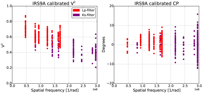
Figure 2: Calibrated squared visibilities (left) and closure phases (right) of IRS 9A. The $V^{2}$ values imply the presence of a partially resolved structure while the CPs are consistent with inversion symmetry of the target.

In this work, we explore the morphology of the MYSO NGC 3603 IRS 9A* (abbreviated hereafter as IRS 9A) with near-infrared interferometric observations and long-slit spectra. The target, which is located in the giant HII region NGC 3603 at a distance of 7$\pm$1 kpc, is a MYSO with an estimated mass of $\sim$ 40 $M_{\odot}$ (Nürnberger 2003). Owing to its location in NGC 3603, the natal cloud of this luminous source ($\sim$ 2.3 x 10${}^{5}L_{\odot}$) has been partially eroded by the stellar radiation of a massive cluster of O and B stars that are located at a projected distance of 2.5 pc to the North-West from the source, thus making it observable at infrared wavelengths. However, its spectral index ($\alpha_{2.2-10\mu m}$=1.37) suggests that the source is still surrounded by considerable circumstellar material. In fact, the observed excess of mid-infrared (MIR) emission, and its positive spectral index, resemble the properties of low-mass class I YSO (Lada 1987; Whitney et al. 2003). This hypothesis of a partially wind-stripped young object offers the intriguing possibility of peering behind the veil at a MYSO during one of its early evolutionary stages.

Previous MIR high angular resolution observations of the IRS 9A morphology identified at least two components that are associated with a warm-inner disk-like structure and a cold elongated envelope with temperatures of $\sim$1000 and $\sim$140 K, respectively (Vehoff et al. 2010). On the one hand, the envelope, resolved with MIR sparse aperture masking (SAM) observations using the T-ReCS IR camera on Gemini South, exhibits an angular size of 330$\times$280 mas. On the other hand, observations with the ESO MIDI instrument, attached to the Very Large Telescope Interferometer (VLTI), implied an angular extension of $\leq 50$ mas for the compact structure.

Here, we make use of SAM data taken with the ESO near-infrared (NIR) facility NACO, at the ESO Very Large Telescope (VLT), to study the morphology at the central region of IRS 9A. These data are complemented with NIR long-slit spectroscopic observations with CRIRES/VLT from the ESO archive. We also reanalyze the existing MIDI/VLTI and T-ReCS/Gemini data, including them in our analysis. The structure of this work is as follows: Section 2 describes the observations and data reduction; our analysis and results for the different used techniques, as well as our models, are presented in Section 3; in Section 4, we discuss our results. Finally, in Section 5 we present our conclusions.

Table 1: Observing log of VLT/NaCo-SAM imaging observations taken on March 12, 2012

Time (UT)	Source	Filter	NDITa	DITb	Camera
05h 05m	IRS 9A	$K_{s}$	8.0	10.0	S27
05h 20m	HD 98194c	$K_{s}$	8.0	10.0	S27
05h 32m	IRS 9A	$K_{s}$	8.0	10.0	S27
05h 46m	HD 98133c	$K_{s}$	8.0	10.0	S27
06h 00m	IRS 9A	$K_{s}$	8.0	10.0	S27
06h 15m	HD 98194c	$K_{s}$	8.0	10.0	S27
06h 27m	IRS 9A	$K_{s}$	8.0	10.0	S27
06h 39m	HD 98133c	$K_{s}$	8.0	10.0	S27
07h 10m	IRS 9A	$L^{\prime}$	126	0.5	L27
07h 22m	HD 97398c	$L^{\prime}$	126	0.5	L27
07h 30m	IRS 9A	$L^{\prime}$	126	0.5	L27
07h 41m	HD 98133c	$L^{\prime}$	126	0.5	L27
07h 50m	IRS 9 A	$L^{\prime}$	126	0.5	L27
08h 02m	HD 97398c	$L^{\prime}$	126	0.5	L27
08h 13m	IRS 9A	$L^{\prime}$	126	0.5	L27
08h 27m	HD 98133c	$L^{\prime}$	126	0.5	L27

• Number of exposures.

• Detector integration time in seconds. The total integration time of each observation amounts to N$\times$DIT$\times$NDIT.

• Stars used as calibrators of the sparse aperture masking data.

2 Observations and data reduction

2.1 Sparse aperture-masking data.

We performed Adaptive Optics (AO) observations of IRS 9A with NACO in its aperture-masking mode using the $K_{s}$ ($2.2\mu m$), $L^{\prime}$ ($3.8\mu m$), and $M^{\prime}$ ($4.7\mu m$) bandpasses on March 12th, 2012 (UTC), combined with the S27/L27 cameras (0.027”/pixel) and the 7holes mask. This mask and configuration are appropriate for use with targets in the magnitude range of IRS 9A. The relatively uniform $u-v$ coverage afforded by this mask yielded a synthesized beam with angular resolution ($\theta$) at each band of 35, 60, and 80 mas for the $K_{s}$, $L^{\prime}$, and $M^{\prime}$ filters, respectively.

Observations were taken using repeated standard calibrator-science target sequences over a period of $\sim$2 hours per filter (see Table 1). Each observation on target and calibrator was composed of four dither positions. Owing to the elevated noise and the presence of vertical stripes in the upper half of the NACO detector at the time of the observations, the dither positions were performed following a squared box in the lower half of the detector. The repeated observation helped to improve our $u-v$ coverage through Earth rotation synthesis (see Fig 1). All SAM data were initially sky subtracted, flat fielded, and bad pixel corrected. For each different position, the sky frames were constructed via separate observations of an empty field close to the target. The sky subtraction did not result in a fully flat background as expected: on the contrary, patterns were found to remain on the images in the $L^{\prime}-$filter. The size of these patterns was larger than the size of the interferogram. Because fringes are encoded at high spatial frequency, we assumed that the effects of these residuals were not significant. Additionally, because of high airmass and variable seeing, the NACO/SAM $M^{\prime}-$filter observations had low photon counts on target, and no interferograms were distinguishable for almost all the recorded data. Therefore the $M^{\prime}-$filter was discarded from our analysis.

To improve the signal-to-noise ratio (S/N), a frame-selection algorithm rejected approximately 50% of the recorded images based on two flux criteria: (i) the total counts on a circular mask of the size of the interferogram, and (ii) the counts at the peak of the interferogram. The final frames were cropped and stored in cubes of 128x128 pixels that were centered on the source peak pixel. Point-source reference stars located not further than 2^∘ from IRS 9A were observed to calibrate the telescope-atmosphere transfer function. Table 1 lists the data sets recorded for both target and calibrators at each observed filter. Figure 1 shows, as an example, the $L^{\prime}-$filter data that gives the average interference pattern over a data cube, the power spectrum, and the final $u-v$ coverage built through Earth-rotation aperture synthesis.

To reduce the raw data to calibrated squared visibilities ($V^{2}$) and closure phases (CPs), an analysis pipeline written in interactive data language (IDL), originally developed at Sydney University, was employed. This code constructs a sampling template (specific to the given configuration of mask and filter) to extract complex visibilities from the Fourier transform domain. Raw interferometric observables are obtained as an average over the data cube for all baselines that were sampled by the mask. Finally, the calibrated amplitudes are obtained through the ratio between raw $V^{2}$ on source and calibrator, while calibrated CPs are obtained by subtracting the CPs of the calibrator from the ones on the target. A more detailed description of the SAM technique can be found in Tuthill et al. (2000, 2010). Additionally, our data were also reduced with the YORICK pipeline for aperture masking (SAMP; Lacour et al. 2011), which was developed at Paris Observatory. Similar results were obtained using both codes.

To test the level of confidence of both the CPs and the $V^{2}$ of our calibrators, we performed a cross-calibration between the different PSF reference stars to determine the response of the interferometric observables and identify systematics. We performed an auto-calibration test for pairs of calibrators taken in the same quadrant of the detector to minimize the difference in the pixel gain of the interferogram and, hence, reduce the variability in the $V^{2}$ level. Our tests confirm that the CPs of the calibrator have individual standard deviations of $\sigma_{CPs}\sim 2^{\circ}$.

Figure 2 presents the calibrated $V^{2}$ and $CPs$ of our IRS 9A $K_{s}$ and $L^{\prime}$ observations. The interferometric observables depict a partially resolved target with point-like symmetry for all the different sampled position angles. The $V^{2}$ levels vary between $\sim$0.4-0.8 and $\sim$0.2-0.7 for $L^{\prime}$ and $K_{s}$, respectively. CPs vary within about -10^∘ and 10^∘ for the two filters.

2.2 CRIRES data

IRS 9A was observed with the CRIRES spectrograph (Käufl et al. 2004) as part of the 080.C-0873(A) observing programme. We obtained these data from the ESO archive. Observations were taken using a grating of 31.6 lines/mm centered on two near-IR emission lines: H₂ (2.121 $\mu$m) and Br_γ (2.166 $\mu$m). The slit length was of $\sim$40” with a plate scale of 0.086”/pixel. The covered dispersion ranges were: 2.108-2.150 and 2.161-2.200 $\mu$m for H₂ and Br_γ, respectively. These observations were conducted using a long-slit with a width of 0.6”, and a resolving power of R$\sim$33000 or 9 km/s. The CRIRES observations were not AO-assisted. To obtain information on the emission lines at different orientations of the target, three position angles (0^∘, 90^∘, and 128^∘) were covered by the slit for each one of the observed lines. The exposure time was 60 s for both observed lines. Two nodding positions, interwoven with sky observations, were taken at each slit position.

The data-reduction was performed using IRAF and proprietary IDL routines. First, the 2D spectrum was corrected for the flat-field, bad pixels, and sky contamination. No strong telluric OH lines were observed at positions threatening to contaminate astrophysically useful lines in the spectra. However, to avoid spurious signals in our data resulting from OH lines, we subtracted the sky observations from the science spectra. After the previous correction, the two nodding positions were aligned along the spatial axis and combined into a single spectrum. To correct for blending along the dispersion axis, a 2nd-degree polynomial was fit to the stellar continuum spectrum, which was then subtracted from the science spectra frames. Figure 5 displays the integrated H₂ and Br_γ emission lines using an aperture of twice the full-width at half-maximum (FWHM) of the continuum emission after processing, as described.

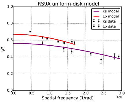
Figure 3: Uniform disk model. The mean-weighted $V^{2}$ data points are represented by black circles and squares for the $Ks$ and $L^{\prime}$ filters, respectively. The red and purple lines represent the best-fit model for the $V^{2}$ in $L^{\prime}$ and $Ks$, respectively.

3 Analysis and results

3.1 The core of IRS 9A probed by K and L-band SAM data

To obtain an estimate of the physical size of the circumstellar structure around the core of IRS 9A, we first fit a geometrical model of a uniform disk to the $V^{2}$ functions from our SAM data. Since we do not completely resolve the compact structure, we omitted the effect of the inclination in the model at this stage. The angular size of the disk obtained with our model is, therefore, an upper limit of the real angular size of the target. The model of a uniform disk in the Fourier space is given by the following expression:

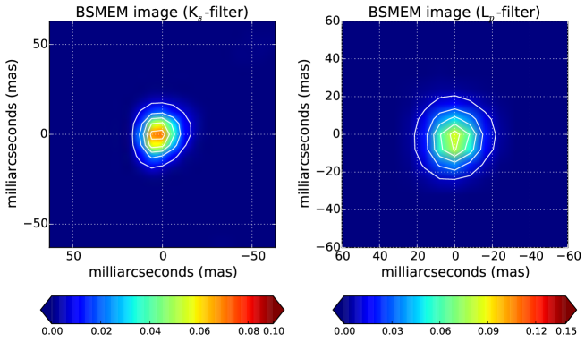
Figure 4: Reconstructed images of IRS 9A from the NACO/SAM data using BSMEM. The left panel shows the image for $K_{s}$ and the right panel the image for $L^{\prime}$. The total flux of the images is normalized to unity. Each panel has overplotted black contours that correspond to 10, 30, 50, 70, 90% of the peak flux.

$$V(u,v)^{2}=\left[\frac{A_{1}}{A_{1}+A_{2}}\right]\left[2\frac{J_{1}(\pi\theta r)}{\pi\theta r}\right]^{2}\,,$$ (1)

where $J_{1}$ is a first order Bessel function, $\theta$ is the diameter of the disk in radians, and $r$ corresponds to the measured spatial frequencies. The coefficient $A_{1}$ corresponds to the squared correlated flux at zero baseline for the disk, and $A_{2}$ to the squared uncorrelated flux, where $A_{1}$+$A_{2}$=1. To optimize the model fit, we used a Levenberg-Marquardt algorithm that was implemented at the IDL $MPFIT$ package (Markwardt 2009). Figure 3 displays the best-fit model obtained for both filters, while Table 2 gives values of the best-fit parameters and their uncertainties. The fact that $A_{1}$ does not reach unity in both bands provides evidence for over-resolved extended flux. Nürnberger (2008) shows the $L^{\prime}-$band large scale structure of the circumstellar environment around IRS 9A. That work presents an East-West elongated emission around IRS 9A with an angular size of around $\sim$1.0-1.5” (or $\sim$7x10³-10x10³ AU at a distance of 7kpc). The angular extension of that diffuse emission is larger than the angular resolution of our shortest baseline ($\theta$=0.5”), consequently, this can explain the origin of the over-resolved flux observed at our NACO/SAM data at $L^{\prime}$. In the case of $K_{s}$, the presence of circumstellar matter or a halo of scattered light could also explain the over-resolved flux that is observed in our interferometric data. This finding will be addressed in subsequent sections.

As well as using the geometrical model, we performed image reconstruction with the calibrated data sets. The maximum entropy code BSMEM was used for this purpose (Buscher 1994). As a prior for the reconstruction, we used the assumption of a uniform disk. The initial model setup included a disk with a diameter of 50 and 100 mas for $K_{S}$ and $L^{\prime}$, respectively. The final images were obtained after 13 and 40 iterations. Figure 4 displays the reconstructed images. As was expected, IRS 9A appears quite compact, however a slight elongation is seen in the East-West direction in the $K_{S}-$filter. On the other hand, at $L^{\prime}$, the source looks quite symmetrical. We note that maximum-entropy (MEM) images usually have a super-resolution beyond the diffraction limit, since the reconstruction depends only on the entropy statistics (for a more detailed description, see Monnier 2003; Monnier & Allen 2013). Images presented in Fig 4 are just the result of the reconstruction and have not been subsequently convolved with any beam to make it more evident that the source does not resemble a point-like object (although it is not completely resolved).

Table 2: Parameters of best-fit uniform-disk model to the $V^{2}$ data

Filter	Parameter	Value	$\sigma^{\mathrm{a}}$
$K_{s}$	$A_{1}^{\mathrm{b}}$	0.56	0.02
	D [mas]c	27.5	2.2
$L^{\prime}$	$A_{1}^{\mathrm{b}}$	0.67	0.02
	D [mas]c	34.2	4.5

• 1-$\sigma$ errors of the best-fit parameters, assuming a reduced $\chi^{2}$ of one.

• $V^{2}$ value at zero-baseline.

• Diameter of the fitted-disk model in units of milliarcseconds.

3.2 The H₂ and Br$\gamma$ spectroastrometric signals

To determine and characterize the region from which H₂ and Br$\gamma$ emission lines arise, we extracted the spectroastrometric (SA) signal from both lines using custom IDL/Python routines. We note that the recommended procedure to calibrate the spectroastrometric signals requires observations with parallel and anti-parallel slit position angles (Brannigan et al. 2006). Since the archival CRIRES data lack anti-parallel position angles, we limit our analysis to the following: Spectroastrometry tracks the centroid of the stellar continuum and of the emission line as a function of wavelength, with an astrometric precision of the order of few milliarcseconds (see Whelan & Garcia 2008). The SA signal was measured on the non-continuum-subtracted data, and recovered by applying a Gaussian fitting to the intensity profile of the observed lines along the spatial axis for each one of the dispersion axis bins.

To eliminate the centroid shift of the SA signal caused by the superposition of the stellar continuum, at the emission line position, we corrected our signal as follows (see Whelan & Garcia 2008; Pontoppidan et al. 2008):

1) The flux of the line ($F_{\lambda(line)}$) was weighted by the sum of the flux of the line and continuum ($F_{\lambda(continuum)}$) according to the following expression:

$$w_{f}=\left[1+\frac{F_{\lambda(continuum)}}{F_{\lambda(line)}}\right].$$ (2)

2) We computed $w_{f}$ using the average value of $F_{\lambda(line)}$ and $F_{\lambda(continuum)}$. The differences in the centroid position between line and continuum were thus multiplied by the computed flux weight, $w_{f}$.

Figure 5 displays the SA signal of the different position angles for both $H_{2}$ and $Br\gamma$ lines. The SA signals, displayed on the histograms, are averaged over three and five spectral bins for H₂ and Br$\gamma$, respectively. All the signals are corrected for the continuum effect, using an average $F_{\lambda(continuum)}$/$F_{\lambda(line)}$ of 0.5 and 0.9 for the Br$\gamma$ and H₂, respectively.

On the one hand, the $Br\gamma$ emission line appears to be formed at the core of IRS 9A with maximum offsets from the continuum of around $\sim$20 mas. On the other hand, in the $H_{2}$ line, the SA signal presents maximum offsets of the order of $\sim$150-300 mas, depending on the position angle of the slit. The sizes of the SA signatures are consistent with the structures observed in our SAM data. This suggests that the central region of IRS 9A has a compact structure that contains ionized material and a more extended surrounding envelope composed of molecular hydrogen.

The maximum shift in the $H_{2}$ SA signal at PA=0^∘ is blue-shifted from the line’s systemic velocity, while the maxima of the shifts in the $H_{2}$ SA signal at PA=90^∘ and PA=128^∘ coincide with the line’s systemic velocity. Since the width of the line profile goes from -10 to 10 km/s, and the spectral resolution of CRIRES is of 9 km/s, the observed line profile merely resembles the response function of the spectrograph. There are two main mechanisms that give rise to the infrared emission of the observed transition, $\nu$=1-0 S(1), in H₂: collisional excitation (e.g., Smith 1995) and ultra-violet (UV) resonant-fluorescence (e.g., Black & van Dishoeck 1987). However, to disentangle which mechanism is responsible for the observed emission line, a test of the flux ratio between the H₂ line at 2.12$\mu$m and the H₂ line at 2.24$\mu$m ($\nu$=2-1 S(1)) will be required (high ratios between those lines implies that the origin of the emission is due to shocked gas and low ratios that the emission is caused by fluorescence; see e.g., Wolfire & Königl 1991).

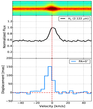
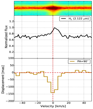
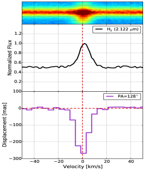
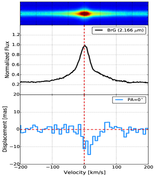
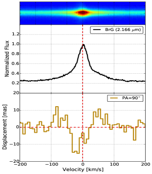
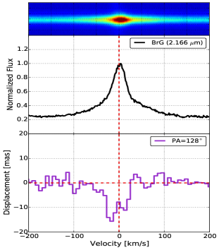
Figure 5: Spectroastrometric signals of the $H_{2}$ and $Br\gamma$ lines of IRS 9A. The $H_{2}$ emission line appears to originate from the large-scale structure of IRS 9A while the $Br\gamma$ line is formed at the core of IRS 9A. The spectroastrometric signal of the line displayed is weighted with $w_{f}$. The mean ratio $F_{\lambda(continuum)}$/$F_{\lambda(line)}$ is of $\sim$0.9 and $\sim$0.5 for the H₂ and the Br$\gamma$ line, respectively. The 2D spectral lines are also displayed in colors.

$Br\gamma$ SA signals at position angles of 90^∘ and 128^∘ exhibit an inverted double-peaked profile, with one of the peaks blue-shifted and the other red-shifted. Velocities at the peaks for both position angles are of about -30 and 30 km/s, respectively. The characteristic SA signature of a disk-like structure shows two peaks that are reversed regarding the direction of their spatial displacement (see e.g., Pontoppidan et al. 2011; Brown et al. 2013; Blanco Cárdenas et al. 2014). Therefore, the observed SA profiles cannot arise from a standard disk-like structure in Keplerian rotation. On the contrary, this type of SA signature appears to be formed in more complex systems with asymmetries. Another intriguing possibility is that the observed Br$\gamma$ SA signal could be explained by the presence of a binary system. Bailey (1998) presented the characterization of several pre-main sequence binaries that exhibit similar SA signals to IRS 9A, finding double-peak profiles, which had been created by binaries, that variate depending on the observed PA; with the maximum shift seen at the position angle of the binary’s orbital plane. Therefore, binarity of the central source may explain the lack of a clear double-peak profile at PA=0^∘. In this scenario, the observed SA signal could be explained by the combined effect of two lines, each one produced by one stellar component, in which one of them exhibits a narrow profile and the other one a broader line-width (see the case of KK Oph in Bailey 1998).

A simple way to determine whether the Br$\gamma$ SA signal is formed of a distribution of material in a common orbital plane (e.g., disk or binary) consists in representing two SA signals observed at different position angles in an x-y 2D plot. If the resulting trend of the astrometric offsets in the x-y plot can be approximated by a linear function, then the material (from which the SA signal is formed) is coplanar, as expected for an orbital plane (see e.g., Bailey 1998; Takami et al. 2003). Figure 6 displays three panels with the x-y maps produced using the observed position angles. The axes plotted in Fig. 6 correspond to the projection in cartesian coordinates of the sampled position angles. As can be seen, neither the x-y plot created with the SA signals on position angles 90^∘ and 0^∘, nor the plot with position angles 128^∘ and 0^∘, yields a linear distribution. The x-y panel formed with PA 128^∘-90^∘ shows a correlation among the signals. However, we suspect that this is caused by the small difference in the displayed position angles. Therefore, we cannot confirm a preferential orbital plane at which the SA signals are formed. In contrast, the observed SA signals appear to represent the contribution of several morphological components of IRS 9A. Similar findings are observed in SA signals of other targets with complex morphologies like the Herbig Ae/Be star Z CMa Bailey (1998). This object shows at least two components with different orbital planes, a binary+disk system with perpendicular outflows, in its 2D spectroastrometric plots.

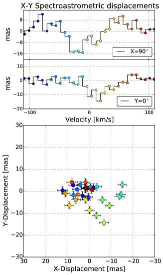
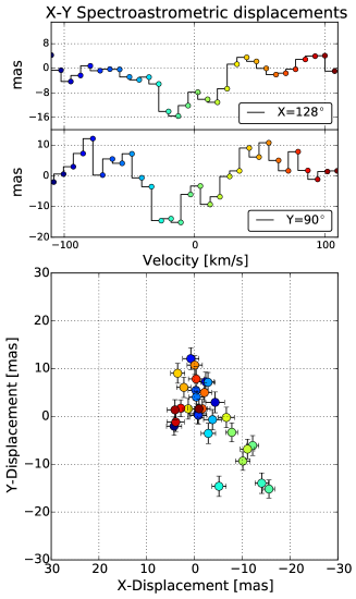
Figure 6: 2D plots of the Br$\gamma$ SA signals. Each panel in the columns represents the flux centroid displacements at two given position angles, as indicated at the top SA signals. Each spectral bin is represented by different colors, the uncertainties in the flux centroid displacements are also plotted.

3.3 IRS 9A radiative transfer model

To determine the physical conditions that best reproduce all the observational information of IRS 9A, we linked the observed $V^{2}$ of our SAM data with the MIR observations from the literature, and the object’s SED through a multi-wavelength radiative transfer simulation. We considered a physical scenario that includes similar properties to the Class I YSO described by Whitney et al. (2003). The structure of the model consists of a compact flared disk around the central source of radiation that is surrounded by an outer, elongated envelope with two bipolar cavities that were probably created by jets and outflows launched at the core of IRS 9A (see Fig. 7). A similar morphology was modeled previously by Vehoff et al. (2010). However, we found that some changes in the reported parameters should be introduced to fit the new NACO/SAM data. The 3D density distribution of the disk in cylindrical coordinates, $\rho_{disk}(R,z,\phi)$, follows a power law described by the expression:

$$\rho_{disk}(R,z,\phi)=\rho_{0}^{disk}\left[\frac{R}{100\,AU}\right]^{\beta+1}exp\left[-1/2\left(\frac{z}{h(R)}\right)^{2}\right],\,$$ (3)

where $\rho_{0}$ is the scale factor of the density, R is the disk radius, and $\beta$ the scale-height disk exponent. The scale-height function is given as: $h(R)=h_{0}(R/R_{0})^{\beta}$. The envelope density distribution corresponds to an elongated structure of infalling material, according to Ulrich (1976). It has the following form:

$$\begin{split}\rho_{env}(R,z,\phi)=\frac{\dot{M}_{envelope}}{4\pi(GM_{*}r_{o})^{1/2}}\left[\frac{r}{r_{0}}\right]^{-3/2}\left[1+\frac{\mu}{\mu_{0}}\right]^{-1/2}\left[\frac{\mu}{\mu_{0}}+\frac{2\mu_{0}^{2}r_{0}}{r}\right]^{-1},\,\end{split}$$ (4)

where r is the radius of the envelope, r₀ is the normalization radius of the envelope, and $\dot{M}$ is the rate of mass infall. The factors $\mu_{0}$ and $\mu$ are related by the equation for the streamline: $\mu_{0}^{3}+\mu_{0}(r/r_{0}-1)-\mu(r/r_{0})=0$. The density distribution in the envelope cavity was considered to be uniform. It is important to emphasize that our simulation does not consider binarity and/or irregularities in the disk at the core of IRS 9A; such detail lies beyond the scope of this work.

To perform the radiative transfer simulation, we used the Hyperion software (Robitaille 2011). This code carries out 3D dust-continuum radiative transfer simulations while creating SEDs and images at the required wavelengths. Our Hyperion simulations used the density distributions of the previously mentioned structures to determine their temperature and flux maps. The code uses a modified random walk (MRW) approximation to propagate the photons in the thickest regions of the simulations. Our model assumes a modified MRN grain-size distribution (Mathis et al. 1977) as determined by Kim et al. (1994). The chemical composition of the dust includes astronomical silicates, graphite, and carbon. The simulated models also include the scattering of the dust with a full numerical approximation to the Stokes parameters in the ray-tracing process. The gas-to-dust ratio of 100:1, a foreground extinction of Av=4.5 (the extinction law used is described in Robitaille et al. (2007)), and a distance of 7 kpc (Nürnberger 2003) were used for all simulations.

From the radiative transfer simulations, we obtained synthetic images of IRS 9A for the $K_{s}$ and $L^{\prime}$ bands, observed with NACO/SAM (see Sec. 3.1), for the $N-$band (11.7 $\mu$m), observed with T-ReCS, and for the MIDI/VLTI (8-13 $\mu$m) data, described in Vehoff et al. (2010). Subsequently, the $V^{2}$ were extracted from those images, at the sampled spatial frequencies by the observations, using proprietary IDL/Python routines. We also obtained synthetic SEDs in the range of 1-500 $\mu$m. For all images, the total flux was normalized according to the angular size of the primary beam.

Table 3: Radiative transfer models of IRS 9A

Parameter	Best SED-only fit a	Vehoff+2010	Best $V^{2}$ model
	(No. 3006825)b	(No. 3012790)b	(this work)
Total luminosity (L⊙)	1.0x105	9.2x104	8.0x104
Stellar mass (M⊙)	27.2	25.4	30.0
Stellar temperature (K)	39000	38500	38000
Disk massc (M⊙)	1.8x10-1	5.0x10-1	5.0x10-1
Disk outer radius (AU)	91.0	94.0	80.0
Disk inner radius (AU)	28.0	25.0	10.0
Disk flaring power -$\beta$-	1.1	1.2	1.2
Disk scale height at 100 AU -$h$-	8.9	8.8	8.0
Envelope outer radius (AU)	1.0x105	1.0x105	7x103
Envelope cavity angle (deg.)d	31.0	29.0	30.0
Bipolar cavity density (g/cm3)	7.7x10-21	9.9x10-21	1.0x10-20
Inclination -$i$- (deg)e	87.0	85.0	60.0
Position Angle -$\phi$- (deg)f	105.0g	105.0	120.0

• This is the best-fit model to the SED obtained with Robitaille’s online fitting tool.

• Number of the model from Robitaille’s database.

• Total mass (dust+gas).

• Half-opening angle of a conical cavity in the envelope.

• Inclination angle of the disk-envelope from the line of sight: 0^∘ means that the disk and envelope are seeing face-on, 90^∘ means that the disk and envelope are seeing edge-on.

• Position angle of the disk mid-plane projected in the plane of the sky, measured East of North.

• Assumed to be the same as Vehoff et al. (2010).

3.3.1 The parameter space

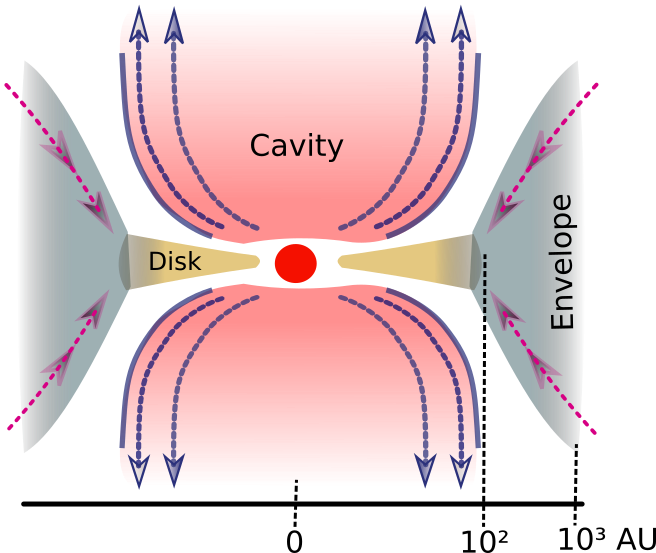
Figure 7: Schematics present the adopted model of the IRS 9A morphology used in our radiative transfer simulations. The model includes an inner disk surrounded by an envelope with bipolar cavities. The purple lines in the cavities indicates the direction of the radiation escaping from the core, while the pink lines in the envelope represent the infall of material from the envelope through the disk. The typical scales of the different components are shown.

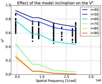
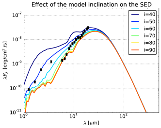
Figure 8: Effect of changing in the inclination angle, $i$, of the model on the simulated $V^{2}$ and SED. On the upper panel, the effect of modifying $i$ on the NACO/SAM $L^{\prime}-$filter is observed. On the lower panel, the effect of changing $i$ over the SED is displayed. The different colors correspond to different values of $i$, while the black dots represent the data in both panels. In this example, the rest of the model parameters remained fixed to the values of the best-fit model presented in this work

To constrain the parameters of our simulation, as a starting point, we used the disk-envelope Vehoff’s model. However, we observed that the new SAM data were not fit by this model. Therefore, some adjustments were necessary to reproduce the observed visibilities. Our intent was not to revisit the full parameter space because the grid of SED models computed by Robitaille et al. (2006) has sampled it quite sparsely for MYSOs. Beginning with Vehoff’s model, we tuned each of the parameters in turn by hand, starting with the inclination and inspecting the fits to visibilities and SED. The tuned parameters are as follows:

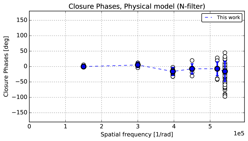
Figure 10: Best-fit of our radiative transfer model to the T-ReCS closure phases. The data are displayed with open black circles and the mean value of the model closure phase is shown with a filled blue circle and with a vertical bar that indicates the variation as a function of azimuth angle.

a) Orientation ($i$, $\phi$): Inclination angle, $i$, of the disk mid-plane from the line of sight was identified as a critical parameter for our modeling. It was noticed that changes in this parameter have a strong impact on the modeled visibilities of the SAM data, besides the changes in the SED and MIR wavelengths. Values of $i$ close to 90^∘ produced systematically low visibilities of the sampled SAM spatial frequencies. On the other hand, values of $i\sim$60^∘ produced simulated visibilities closer to the expected SAM values. Figure 8 displays the effect of inclination on the simulated V² for the $L^{\prime}-$filter and SED for different values of $i$ between 40^∘ and 90^∘ in steps of 10^∘. From these results, we found that an average value of $i$=60^∘ best-fit the different data sets. To obtain the position angle, $\phi$, of the mid-plane of the disk in the plane of the sky, we rotate our projected model in intervals of 10^∘ from $\phi$=0^∘ to $\phi$=360^∘. Since the lack of phase information in the MIDI data and that the NACO/SAM closure phases were not sensitive to the projected position angle (because IRS 9A was only partially resolved; see Fig. 2), we adopted the value of $\phi$ that minimizes the residuals of V² and CPs of the T-ReCS data. In this case $\phi$=120^∘ (see Figs. 10 and 12).

b) The central source ($T_{eff}$, $L_{*}$, $M_{*}$): As established in Vehoff et al. (2010), the model assumes the typical stellar parameters of a main-sequence O-star (see e.g., Martins et al. 2005). The effective temperature was thus fixed at $T_{eff}=$38000 K and the mass to M$=$30M_⊙. Only variations of the luminosity were performed in steps of 1x10${}^{4}L_{\odot}$ from $L_{*}=$1.0x10${}^{5}L_{\odot}$ to 8x10${}^{4}L_{\odot}$ to have a reasonable fitting to the SED.

c) The disk ($R_{in}$, $R_{out}$, $m_{disk}$, $\beta$, $h_{0}$): The inner radius of the disk was obtained from variations of the value given by Vehoff et al. (2010). The covered values went from 10 to 25 mas in increments of 5 mas. The value that best reproduce the observed $V^{2}$ is $R_{in}$=10 mas. This value is in agreement with the sublimation radius of the dust (for a sublimation temperature $T_{sub}=$1500 K) according to Monnier & Millan-Gabet (2002):

$$R_{sub,disk}=1.1\sqrt{Q_{R}}\left[\frac{L*}{1000L_{\odot}}\right]^{1/2}\left[\frac{T_{sub}}{1500K}\right]^{-2}\leavevmode\nobreak\ AU\,\,$$ (5)

Considering a ratio of the dust absorption efficiencies $Q_{R}$=1, the inner radius was thus estimated as: $R_{in}$=$R_{sub,disk}$=10 AU. On the other hand, the initial value of the outer radius was fixed to $R_{out}$=100 AU, since this was the value derived from the geometrical model (R$\sim$14 mas $\sim$ 98 AU) described in section 3.1. Variations of $R_{out}$ were performed in steps of 10 AU from 40 to 100 AU. We observed that changes in this range do not have a strong impact on the simulated SED, and that they only introduced slight changes in the simulated $V^{2}$ within the scatter of the observed $V^{2}$. Therefore, we adopted an average value of $R_{out}$=80 AU. For the mass of the disk and the flaring exponent, $\beta$, we used the same values as Vehoff et al. (2010), thus $m_{disk}$=5x10^-3M_⊙ and $\beta$=1.2, respectively. To determine the scale height, $h_{0}$, at 100 AU, we performed several tests with values of $h_{0}$ between 3-10 AU, with steps of 1 AU, finding that the value that best reproduces the visibilities is $h_{0}$ =8 AU, which is very close to the value previously reported by Vehoff et al. (2010).

Figure 9: Models of IRS 9A, giving predicted $V^{2}$ at NIR and MIR wavelengths. The model signals are displayed with varying linetypes (see key). The data are displayed with open black circles. At each spatial frequency for the $K_{s}$, $L^{\prime}$, and $N$ data sets, the mean value of the model visibility is shown with a filled blue circle, and with a vertical bar that indicates the variation as a function of azimuth angle.

d) Envelope and cavities ($\phi$, $\rho_{cav}$, $R_{out,cav}$): The parameters of the envelope and cavities were adopted from Vehoff et al. (2010). The value of the opening angle of the cavity ($\phi$) was fixed to 30^∘, and the density ($\rho_{cav}$) to 1x10^-20 g/cm³. For the envelope, we adopted a normalization radius of 100 AU and an outer radius of 7x10³AU (1”). The scale of the outer radius was inferred from the extension observed at MIR wavelengths, which exhibit an angular scale of around 1”. Tests with larger $R_{out,cav}$, like the value reported by Vehoff et al. (2010), produced visibilities systematically below the observed levels, and were therefore discarded.

Figure 9 presents a comparison of the V² fitting of (i) our best-fit model with (ii) the model of the MIR morphology of IRS 9A presented by Vehoff et al. (2010), and with (iii) the best-fit model of the IRS 9A SED that was obtained with Robitaille’s online fitting tool (Robitaille et al. 2007). Vehoff’s model was also obtained from Robitaille’s tool, but it does not correspond to the best-fit model delivered by the online database for the used data, although it does provide a reasonable fit to the MIR visibilities. We included both models in Fig. 9 for completeness. Remarkably, the model of Vehoff et al. (2010), analyzed here, has a maximum angular size at zero spacing of $\sim$2”. Caution is recommended when making comparisons to Fig. 6 of Vehoff et al. (2010), since these authors limited the maximum size to 0.85”, which lead to bias in the simulated T-ReCS visibilities of the shortest baselines. Table 3 displays the parameters of each model. Figure 11 displays the SED of IRS 9A for each of the models plotted over the observational data. The NIR photometry was taken from Nürnberger (2003) and the MIR one from Vehoff et al. (2010). Fig 12 displays an RGB image, composed from our models at 2.2, 3.8, and 11.7 $\mu$m.

Table 4: Comparison of the root mean square error (RMSError) between the different models of IRS 9A

Data set	Best SED-only fita	Vehoff+2010	Best $V^{2}$ model
	(No. 3006825)	(No. 3012790)	(this work)
NACO/SAM $K_{s}-$filter	6.3	6.3	3.1
NACO/SAM $L^{\prime}-$filter	25.2	25.4	4.9
T-ReCS data	20.4	20.0	9.4
MIDI data	8.4	4.4	3.5
SED	2.29	2.98	3.4

• This is the best-fit model to the SED, obtained with Robitaille’s online fitting tool.

4 Discussion

As shown in Fig. 9, the model presented by Vehoff et al. (2010), which is based on the MIR data, does not reproduce the observed $V^{2}$ signals extracted from the new NIR SAM observations. In fact, that model is shifted systematically towards lower $V^{2}$ values at the three $K_{s}$, $L^{\prime}$, and $N$ bands. Similar $V^{2}$ misfits have been observed for the model obtained with Robitaille’s online tool, which was based only on the SED data. To perform a more quantitative comparison between the different models, we computed the root mean squared error (RMSError) for each $V^{2}$ data set and SED. Table 4 displays the obtained RMSError for the different models and data sets. We note how the model presented in this work exhibits considerably lower residuals than the other two models for the NACO/SAM and T-ReCS data. However, the residuals of our model are similar to the ones presented by the other two models for the MIDI data.

From Fig. 11 it is appreciated that, despite this poor performance when confronted with the interferometric data, good fits to the SED are exhibited by both Robitaille and Vehoff models. In fact, our model presents the highest residuals. Nevertheless, this result is not unexpected since SED fitting alone often offers highly degenerate outcomes: strong constraints are only provided when SEDs are used in concert with spatial information that identifies the origin of the emission. For example, even single envelope models are sufficient to reproduce the observed SED, although none reproduce, simultaneously, the observed $V^{2}$. Furthermore, the apertures used to extract the SED measurements are considerably larger (3”) than the angular size of IRS 9A. Therefore, some measurements may be contaminated by flux from nearby sources in the field (see, e.g., Fig 2 in Nürnberger 2008, in which additional sources are observed around IRS 9A in a radius of $\sim$3”). This underlines the importance of obtaining SED data at adequate angular resolution, as well as multi-wavelength interferometric observations, combined with SED modeling, to construct a reliable physical framework of the MYSOs morphology.

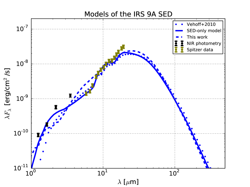
Figure 11: Comparison between the various different so-called best-fit (see text) models to the IRS 9A SED. The photometry data are displayed in black and green. The different models are shown in blue (see the caption inside the plot). The SED models are displayed, assuming an aperture of 3” at a distance of 7.0 kpc and A_v=4.5.

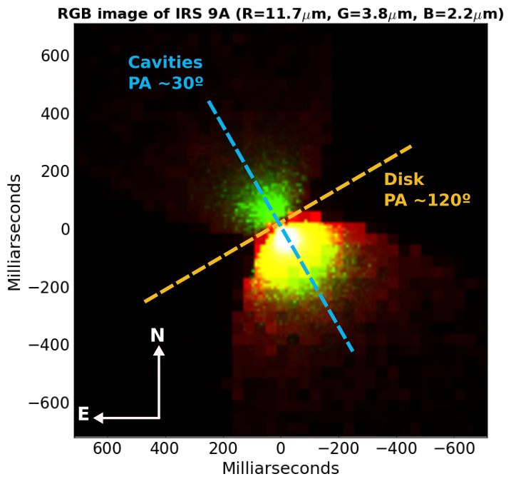
Figure 12: RGB image composed with our model. Note how the emission arises from the cavities that dominate the IR. The red, green, and blue filters correspond to the images of the models at 11.7 $\mu$m, 3.8 $\mu$m, and 2.2 $\mu$m. The position angles (measured East to the North) of the disk and cavities in the plane of the sky are shown.

In contrast to previous works, we have produced a model of IRS 9A that reproduces all observable data, including $V^{2}$ signals at NIR and MIR wavelengths (although some deviations are present at the shortest baselines of the $K_{s}$ and $L^{\prime}$ filters and in the largest baselines of the MIDI data). Our model reproduces the longest baseline visibilities from the T-ReCS data, but underestimates V² at the shortest T-ReCS baselines. We emphasise that, in contrast to the other filters, the N-band T-ReCS data sample the largest scale of IRS 9A. Therefore, we infer that our model faithfully reproduces IRS 9A morphology up to scales $\leq$ 1” (7000 AU), but significantly differs from the V² data that correspond to angular scales between 1”-1.6” (7000-11000 AU). In fact, from the reconstructed T-ReCS/SAM image presented in Vehoff et al. (2010), it is noticeable that the morphology of IRS 9A at larger scales is irregular and more complex than our modeling.

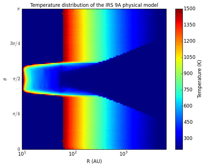
Figure 13: Radial cut of the temperature distribution of the dust around IRS 9A. The picture displays the temperature profile of the disk and the envelope obtained with our best radiative transfer model. The axis is given in spherical coordinates (R, $\theta$) and the colors represent different temperature values of the dust. Also, confusion with other (extended or stellar) sources in the crowded IRS 9 region may be an important source of bias in the SED at certain wavelengths.

Figure 13 displays a radial slice through the temperature distribution of our best model. It is observed that the disk atmosphere has a temperature close to the dust sublimation limit (T$\sim$1500 K) while the mid-plane regions of the disk have an average temperature around T$\sim$600 K. Our simulation also suggests that regions closer than 2 mas (10 AU) to the central source are dust-free because processes, such as the stellar radiation and/or self-heating of the disk, sublimate the dust at these scales (see, e.g., Vaidya et al. 2009).

With regard to the origin of the emission that is observed in the IRS 9A SED, Figure 14 shows the thermal and scattering contributions from the best-fit physical model. This plot indicates that scattered photons from the stellar source are the most important source of radiation at the $K_{s}$-filter, and that they also contribute to the emission observed at the $L^{\prime}$-filter, while thermal emission from the dust dominates the mid- and far-infrared.

5 Conclusions

We summarise our conclusions as follows:

a) The analytical model of a Class I YSO, described by Whitney et al. (2003), appears to be a relatively good approximation of IRS 9A morphology. This source appears to be an embedded object that is surrounded by a thick envelope, which dominates the spectral energy distribution, and with a flat plausibly disk-like structure at its center. This result supports contemporary thinking in star formation, which suggest that massive stars gain mass via accretion disks that shield part of the infalling material from the strong radiation pressure.

b) From our NACO/SAM data, we have confirmed the presence of a compact , possibly disk-like, structure with an angular size $\leq$30 mas. From our radiative transfer simulations, we have found that this structure is responsible for most of the NIR flux distribution of the IRS 9A SED.

c) From our best-fit radiative transfer model, we have found that the large scale MIR emission is dominated by the heated dust within the envelope cavity. This is particularly supported by the observed morphology at 11.7 $\mu$m with T-ReCS. The model envelope has an angular size of $\sim$ 1”. Owing to the high luminosity of the central source, the hot inner regions of the envelope also emit at NIR wavelengths.

d) The observed extended emission in the $L^{\prime}-$filter NACO image that was presented by Nürnberger (2008) is the most plausible reasoning for the over-resolved emission observed in the $K_{s}$ and $L^{\prime}$ squared visibility signals.

e) Our best physical model suggests that the system of disk+envelope is inclined $\sim$60^∘ out of the plane of the sky, where 0^∘ corresponds to a face-on orientation of the disk. Moreover, from our simulations, we find that smaller inclination angles generate a large bump at near-IR wavelengths and $V^{2}$ close to unity. Higher inclinations, as suggested in prior literature models, produce low $V^{2}$ (failing to reproduce the data). A fit of our model to the T-ReCS V² and CPs allowed us to constraint $\phi\sim$120^∘, a value close to the 105^∘ (geometric Ring + Gaussian) previously reported by Vehoff et al. (2010).

f) From the Br$\gamma$ spectroastrometric signal, we have found that the core of IRS 9A is complex with ionized gas arising from different regions (with sizes of $\sim$10 mas or $\sim$60 AU) of the morphology. New optimized spectroastrometric observations and interferometric observations with GRAVITY/VLTI and/or MATISSE/VLTI, combined with radiative transfer emission line models, may be useful in confirming this hypothesis and search for the presence of additional stellar companions at the core of IRS 9A.

g) A complete self-consistent physical scenario to describe IRS 9A’s complex morphology is challenging, in particular fitting both the spectral energy distribution and both small-/large-scale spatial structure. However, systems such as this one represent important and rare test cases with which to confront theoretical models. In this work, we have demonstrated that a multi-wavelength approach is necessary to unveil the physical and geometrical properties of MYSOs. Our results indicate that optical interferometry and spectroastrometry are important observing techniques to map the morphological properties at the core of these targets, where important physical phenomena occur.

h) Future work will require more data with optical interferometry and spectroastrometry to refine the existing models. Moreover, additional data at longer wavelengths (e.g., observations with ALMA) are also necessary to better constrain the Rayleigh-Jeans part of the SED, and to obtain more accurate information of the size and density of the envelope. Similar analysis should be extended to other MYSOs to systematically study their properties, driving further incisive testing of massive star formation scenarios.

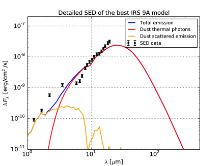
Figure 14: Spectral energy distribution of the best-fit radiative transfer model (blue line). The thermal and scattering contributions are displayed separately in red and yellow linetype respectively.