Unsolved Problems in Virtual Knot Theory and Combinatorial Knot Theory

Abstract

This paper is a concise introduction to virtual knot theory, coupled with a list of research problems in this field.

1 Introduction

The purpose of this paper is to give an introduction to virtual knot theory and to record a collection of research problems that the authors have found fascinating. The second section of the paper introduces the theory and discusses some problems in that context. Starting from the third sections, we present specific problems. This paper is an expanded and revised version of our earlier paper on the subject of problems in virtual knot theory (see [47]). Here we include a wider selection of problems, including some problems of a combinatorial flavor in classical knot theory and other problems in extensions and variants of the theory of knots and links.

We would like to take this opportunity to acknowledge the many people who have worked on the theory of virtual knots and links.

Researchers in this area explicitly mentioned or referenced in this paper are: R. S. Avdeev, V. G. Bardakov, A. Bartholomew, D. Bar-Natan, S. Budden, S. Carter, K. Chu, M. W. Chrisman, H. Dye, R. Fenn, R. Furmaniak, M. Gousssarov, J. Green, A. Henrich, D. Hrencecin, D. P. Ilyutko, D. Jelsovsky, M. Jordan, T. Kadokami, A. Kaestner, N. Kamada, S. Kamada, L. Kauffman, T. Kishino, G. Kuperberg, S. Lambropoulou, V. O. Manturov, S. Nelson, M. Polyak, D. E. Radford, S. Satoh, J. Sawollek, M. Saito, W. Schellhorn, D. Silver, V. Turaev, V. V. Vershinin, O. Viro, S. Williams, P. Zinn-Justin and J. B. Zuber. See [1, 2, 3, 5, 9, 11, 14, 15, 16, 17, 18, 19, 20, 21, 22, 23, 24, 25, 26, 27, 28, 29, 30, 31, 32, 33, 34, 35, 36, 37, 38, 39, 40, 42, 46, 47, 48, 49, 50, 51, 52, 53, 54, 55, 60, 64, 65, 67, 68, 69, 70, 71, 72, 73, 74, 79, 81, 82, 83, 84, 85, 93, 94, 96, 97, 99, 100, 101, 102, 103, 106, 109, 110, 111, 112, 113, 114, 119, 120, 124, 125, 132, 133, 134, 137, 138, 147, 148, 149, 150, 151, 152, 153, 154, 155, 156, 157, 158, 159, 160, 161, 162, 163, 164, 165, 166, 167, 168, 169, 170, 171, 172, 173, 174, 175, 176, 177, 178, 179, 180, 181, 182, 183, 184, 190, 191, 200, 201, 202, 203, 204, 205, 206, 207, 211, 212, 214, 218, 222, 223]. We apologize to anyone who was left out of this list of participant researchers, and we hope that the problems described herein will stimulate people on and off this list to enjoy the beauty of virtual knot theory!

2 Knot Theories

2.1 Virtual knot theory

Knot theory studies the embeddings of curves in three-dimensional space. Virtual knot theory studies the embeddings of curves in thickened surfaces of arbitrary genus, up to the addition and removal of empty handles from the surface. Virtual knots have a special diagrammatic theory that makes handling them very similar to the handling of classical knot diagrams. In fact, this diagrammatic theory simply involves adding a new type of crossing to the knot diagrams, a virtual crossing that is neither under nor over. From a combinatorial point of view, the virtual crossings are artifacts of the representation of the virtual knot or link in the plane. The extension of the Reidemeister moves that takes care of them respects this viewpoint. A virtual crossing (see Fig. 1) is represented by two crossing arcs with a small circle placed around the crossing point.

Moves on virtual diagrams generalize the Reidemeister moves for classical knot and link diagrams, see Fig. 1. One can summarize the moves on virtual diagrams by saying that the classical crossings interact with one another according to the usual Reidemeister moves. One adds the detour moves for consecutive sequences of virtual crossings and this completes the description of the moves on virtual diagrams. It is a consequence of moves (B) and (C) in Fig. 1 that an arc going through any consecutive sequence of virtual crossings can be moved anywhere in the diagram keeping the endpoints fixed; the places where the moved arc crosses the diagram become new virtual crossings. This replacement is the detour move, see Fig. 2.

One can generalize many structures in classical knot theory to the virtual domain, and use the virtual knots to test the limits of classical problems such as the question whether the Jones polynomial [41, 76, 77, 78, 81, 82, 87, 89, 115, 189, 221] detects knots and other classical problems. Counterexamples often exist in the virtual domain, and it is an open problem whether these counterexamples are equivalent (by addition and subtraction of empty handles) to classical knots and links. Virtual knot theory is a significant domain to be investigated for its own sake and for a deeper understanding of classical knot theory.

Another way to understand the meaning of virtual diagrams is to regard them as representatives for oriented Gauss codes (Gauss diagrams) [60, 91, 93]. Such codes do not always have planar realizations and an attempt to embed such a code in the plane leads to the production of the virtual crossings. The detour move makes the particular choice of virtual crossings irrelevant. Virtual equivalence is the same as the equivalence relation generated on the collection of oriented Gauss codes modulo an abstract set of Reidemeister moves on the codes.

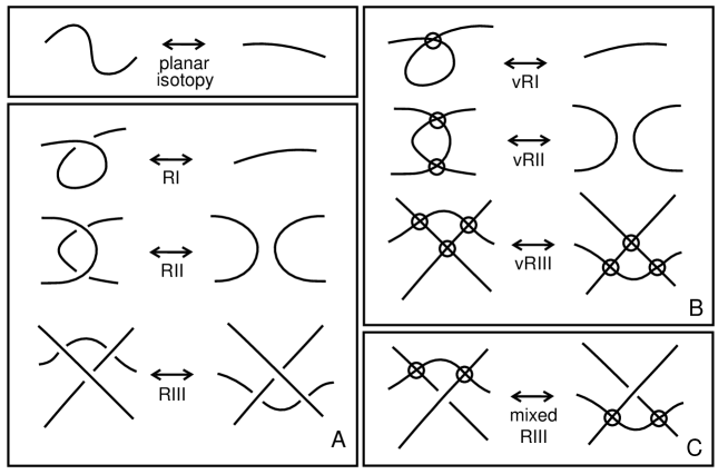
Figure 1: Generalized Reidemeister moves for virtual knots

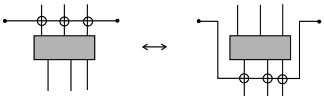
Figure 2: Detour Move

2.2 Flat virtual knots and links

Every classical knot or link diagram can be regarded as a $4$-regular plane graph with extra structure at the nodes. This extra structure is usually indicated by the over and under crossing conventions that give instructions for constructing an embedding of the link in three dimensional space from the diagram. If we take the diagram without this extra structure, it is the shadow of some link in three dimensional space, but the weaving of that link is not specified. It is well known that if one is allowed to apply the Reidemeister moves to such a shadow (without regard to the types of crossing since they are not specified) then the shadow can be reduced to a disjoint union of circles. This reduction is no longer true for virtual links. More precisely, let a flat virtual diagram be a diagram with virtual crossings as we have described them and flat crossings consisting in undecorated nodes of the $4$-regular plane graph. Virtual crossings are flat crossings that have been decorated by a small circle. Two flat virtual diagrams are equivalent if there is a sequence of generalized flat Reidemeister moves (as illustrated in Fig. 1) taking one to the other. A generalized flat Reidemeister move is any move as shown in Fig. 1, but one can ignore the over or under crossing structure. Note that in studying flat virtual knots the rules for changing virtual crossings among themselves and the rules for changing flat crossings among themselves are identical. However, detour moves as in Fig. 1C are available for virtual crossings with respect to flat crossings and not the other way around.

We shall say that a virtual diagram overlies a flat diagram if the virtual diagram is obtained from the flat diagram by choosing a crossing type for each flat crossing in the virtual diagram. To each virtual diagram $K$ there is an associated flat diagram $F(K)$ that is obtained by forgetting the extra structure at the classical crossings in $K.$ Note that if $K$ is equivalent to $K^{\prime}$ as virtual diagrams, then $F(K)$ is equivalent to $F(K^{\prime})$ as flat virtual diagrams. Thus, if we can show that $F(K)$ is not reducible to a disjoint union of circles, then it will follow that $K$ is a non-trivial virtual link.

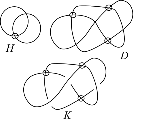
Figure 3: Flats $H$ and $D$, and the knot $K$

Fig. 3 illustrates an example of a flat virtual link $H.$ This link cannot be undone in the flat category because it has an odd number of virtual crossings between its two components and each generalized Reidemeister move preserves the parity of the number of virtual crossings between components. Also illustrated in Fig. 3 is a flat diagram $D$ and a virtual knot $K$ that overlies it. This example is given in [93]. The knot shown is undetectable by many invariants (fundamental group, Jones polynomial) but it is knotted. The flat virtual diagrams present a challenge for the construction of new invariants. It is important to understand the structure of flat virtual knots and links. This structure lies at the heart of the comparison of classical and virtual links. Simpler and more fundamental than flat virtual knots and links are the free knots and links [175, 176] corresponding to Gauss diagrams with no signs and no arrows. We will list a number of problems about free knots below.

2.3 Interpretation of virtual knots as stable classes of links in thickened surfaces

There is a useful topological interpretation for this virtual theory in terms of embeddings of links in thickened surfaces, see [93, 97, 138]. Regard each virtual crossing as a shorthand for a detour of one of the arcs in the crossing through a $1$-handle that has been attached to the 2-sphere of the original diagram. By interpreting each virtual crossing in this way, we obtain an embedding of a collection of circles into a thickened surface $S_{g}\times\mathbb{R}$, where $g$ is the number of virtual crossings in the original diagram $L$, $S_{g}$ is a compact oriented surface of genus $g$ and $\mathbb{R}$ denotes the real line. We say that two such surface embeddings are stably equivalent if one can be obtained from another by isotopy in the thickened surfaces, homeomorphisms of the surfaces and the addition or subtraction of empty handles. Then we have the following theorem.

Theorem 2.1 (see [93, 107, 138]).

Two virtual link diagrams are equivalent if and only if their correspondent surface embeddings are stably equivalent.

Here long knots (or, equivalently $1-1$ tangles) come into play. Having a knot, we can break it at some point and take its ends to infinity (say, in a way that they coincide with the horizontal axis line in the plane). One can study isotopy classes of such knots. A well-known theorem says that in the classical case, knot theory coincides with long knot theory. However, this is not the case for virtual knots. By breaking the same virtual knot at different points, one can obtain non-isotopic long knots [7, 163]. Furthermore, even if the initial knot is trivial, the resulting long knot may not be trivial. A connected sum of two trivial virtual diagrams may not be trivial in the compact case. The phenomenon occurs because these two knot diagrams may be non-trivial in the long category. It is sometimes more convenient to consider long virtual knots rather than compact virtual knots, since connected sum is well-defined for long knots.

Unlike classical knots, the connected sum of long virtual knots is not commutative [7, 162, 163]. Thus, if we show that two long knots $K_{1}$ and $K_{2}$ do not commute, then we see that they are different and both non-classical.

A typical example of such knots is the two parts of the Kishino knot, see Fig. 4.

Figure 4: Kishino and parts

We have a natural map

$$\langle\mbox{Long virtual knots }\rangle\to\langle\mbox{Oriented compact virtual knots}\rangle,$$

obtained by taking two infinite ends of the long knots together to make a compact knot. This map is obviously well defined.

Note that when the parts of the Kishino knot are closed they become unknots.

This map allows one to construct long virtual knot invariants from classical invariants, i.e., just to regard compact knot invariants as long knot invariants. There is no well-defined inverse for this map. The long category can also be applied for the case of flat virtual knots, where all problems formulated above occur as well.

3 Switching and Virtualizing

Given a crossing $i$ in a link diagram, we define $s(i)$ to be the result of switching that crossing so that the undercrossing arc becomes an overcrossing arc and vice versa. We also define the virtualization $v(i)$ of the crossing by the local replacement indicated in Fig. 5. In this figure we illustrate how in the virtualization of the crossing the original crossing is replaced by a crossing that is flanked by two virtual crossings.

Suppose that $K$ is a (virtual or classical) diagram with a classical crossing labeled $i.$ Let $K^{v(i)}$ be the diagram obtained from $K$ by virtualizing the crossing $i$ while leaving the rest of the diagram just as before. Let $K^{s(i)}$ be the diagram obtained from $K$ by switching the crossing $i$ while leaving the rest of the diagram just as before. Then it follows directly from the definition of the Jones polynomial that

$$V_{K^{s(i)}}(t)=V_{K^{v(i)}}(t).$$

As far as the Jones polynomial is concerned, switching a crossing and virtualizing a crossing look the same.

The involutory quandle [90] is an algebraic invariant equivalent to the fundamental group of the double branched cover of a knot or link in the classical case. In this algebraic system one associates a generator of the algebra $IQ(K)$ to each arc of the diagram $K$ and there is a relation of the form $c=ab$ at each crossing, where $ab$ denotes the (non-associative) algebra product of $a$ and $b$ in $IQ(K).$ See Fig. 6. In this Figure we have illustrated through the local relations the fact that

$$IQ(K^{v(i)})=IQ(K).$$

As far the involutory quandle is concerned, the original crossing and the virtualized crossing look the same.

If a classical knot is actually knotted, then its involutory quandle is non-trivial [220]. Hence if we start with a non-trivial classical knot, we can virtualize any subset of its crossings to obtain a virtual knot that is still non-trivial. There is a subset $A$ of the crossings of a classical knot $K$ such that the knot $SK$ obtained by switching these crossings is an unknot. Let $Virt(K)$ denote the virtual diagram obtained from $A$ by virtualizing the crossings in the subset $A.$ By the above discussion the Jones polynomial of $Virt(K)$ is the same as the Jones polynomial of $SK$, and this is $1$ since $SK$ is unknotted. On the other hand, the $IQ$ of $Virt(K)$ is the same as the $IQ$ of $K$, and hence if $K$ is knotted, then so is $Virt(K).$ We have shown that $Virt(K)$ is a non-trivial virtual knot with unit Jones polynomial. This completes the proof of the theorem.

Figure 5: Switching and virtualizing a crossing

Figure 6: $IQ(Virt(K))=IQ(K)$

If there exists a classical knot with unit Jones polynomial, then one of the knots $Virt(K)$ produced by this theorem may be equivalent to a classical knot. It is an intricate task to verify that specific examples of $Virt(K)$ are not classical.

A very fruitful line of new invariants comes about by examining a generalization of the fundamental group or quandle that we call the biquandle of the virtual knot. The biquandle is discussed in the next Section. Invariants of flat knots (when one has them) are useful in this regard. If we can verify that the flat knot $F(Virt(K))$ is non-trivial, then $Virt(K)$ is non-classical. In this way the search for classical knots with unit Jones polynomial (see [211] for links) expands to the exploration of the structure of the infinite collection of virtual knots with unit Jones polynomial.

Another way of putting this theorem is as follows: In the arena of knots in thickened surfaces there are many examples of knots with unit Jones polynomial. Might one of these be equivalent via handle stabilization to a classical knot? In [138] Kuperberg shows the uniqueness of the embedding of minimal genus in the stable class for a given virtual link. The minimal embedding genus can be strictly less than the number of virtual crossings in a diagram for the link. There are many problems associated with this phenomenon.

4 Atoms

An atom is a pair: $(M^{2},\Gamma)$ where $M^{2}$ is a closed $2$-manifold and $\Gamma$ is a 4-valent graph in $M^{2}$ dividing $M^{2}$ into cells such that these cells admit a checkerboard coloring (the coloring is also fixed). $\Gamma$ is called the frame of the atom, see [56, 57, 58, 59, 145, 146, 162, 164].

Atoms are considered up to natural equivalence, that is, up to homeomorphisms of the underlying manifold $M^{2}$ mapping the frame to the frame and black cells to black cells. From this point of view, an atom can be recovered from the frame together with the following combinatorial structure:

1. $A$-structure: This indicates which edges for each vertex are opposite edges. That is, it indicates the cyclic structure at the vertex.

2. $B$-structure: This indicates pairs of “black angles”. That is, one divides the four edges emanating from each vertex into two sets of adjacent (not opposite) edges such that the black cells are locally attached along these pairs of adjacent edges.

Given a virtual knot diagram which has its regions black and white colored like a chess board, one can construct the corresponding atom as follows. Classical crossings correspond to the vertices of the atom, and generate both the $A$-structure and the $B$-structure at these vertices (the $B$-structure comes from over/under information). Thus, an atom is uniquely determined by a virtual knot diagram. It is easy to see that the inverse operation is well defined modulo virtualization. Thus the atom knows everything about the bracket polynomial (Jones polynomial) of the virtual link.

The crucial notions here are the minimal genus of the atom and the orientability of the atom. For instance, for each link diagram with a corresponding orientable atom (all classical link diagrams are in this class), all degrees of the bracket are congruent modulo four while in the non-orientable case they are congruent only modulo two.

The orientability condition is crucial in the construction of the Khovanov homology theory for virtual links as in [162, 164].

5 Biquandles

5.1 Main constructions

In this section we give a sketch of some recent approaches to invariants of virtual knots and links.

A biquandle [5, 14, 19, 46, 97, 124] is an algebra with four binary operations written $a^{b},\,a_{b},\,a^{\overline{b}},\,a_{\overline{b}}$ together with some relations which we will indicate below. The fundamental biquandle is associated with a link diagram and is invariant under the generalized Reidemeister moves for virtual knots and links. The operations in this algebra are motivated by the formation of labels for the edges of the diagram, see Fig 7. In this figure we have shown the format for the operations in a biquandle. The overcrossing arc has two labels, one on each side of the crossing. There is an algebra element labeling each edge of the diagram. An edge of the diagram corresponds to an edge of the underlying plane graph of that diagram.

Let the edges oriented toward a crossing in a diagram be called the input edges for the crossing, and the edges oriented away from the crossing be called the output edges for the crossing. Let $a$ and $b$ be the input edges for a positive crossing, with $a$ the label of the undercrossing input and $b$ the label on the overcrossing input. In the biquandle, we label the undercrossing output by

$$c=a^{b},$$

while the overcrossing output is labeled

$$d=b_{a}.$$

The labelling for the negative crossing is similar using the other two operations.

To form the fundamental biquandle, $BQ(K)$, we take one generator for each edge of the diagram and two relations at each crossing (as described above).

Figure 7: Biquandle relations at a crossing

Another way to write this formalism for the biquandle is as follows

$$a^{b}=a\,\leavevmode\hbox{\lower 3.4pt\hbox{\vbox{\hrule height=0.4pt\hbox{ \hskip 3.0pt\vbox{\vskip 3.0pt\hbox{b}\vskip 3.0pt}\hskip 3.0pt\vrule width=0.4pt}}}},\,a_{b}=a\,\leavevmode\hbox{\lower 3.4pt\hbox{\vbox{ \hbox{ \hskip 3.0pt\vbox{\vskip 3.0pt\hbox{b}\vskip 3.0pt}\hskip 3.0pt\vrule width=0.4pt}\hrule height=0.4pt}}},\,a^{\overline{b}}=a\,\leavevmode\hbox{\lower 3.4pt\hbox{\vbox{\hrule height=0.4pt\hbox{\vrule width=0.4pt\hskip 3.0pt\vbox{\vskip 3.0pt\hbox{b}\vskip 3.0pt}\hskip 3.0pt}}}},\,a_{\overline{b}}=a\,\leavevmode\hbox{\lower 3.4pt\hbox{\vbox{ \hbox{\vrule width=0.4pt\hskip 3.0pt\vbox{\vskip 3.0pt\hbox{b}\vskip 3.0pt}\hskip 3.0pt}\hrule height=0.4pt}}}.$$

We call this the operator formalism for the biquandle.

These considerations lead to the following definition.

• 5.1. A biquandle $B$ is a set with four binary operations indicated above: $a^{b}\,\mbox{,}\,a^{\overline{b}}\,\mbox{,}\,a_{b}\,\mbox{,}\,a_{\overline{b}}.$ We shall refer to the operations with barred variables as the left operations and the operations without barred variables as the right operations. The biquandle is closed under these operations and the following axioms are satisfied:

  1. Given an element $a$ in $B$, then there exists an $x$ in the biquandle such that $x=a_{x}$ and $a=x^{a}.$ There also exists a $y$ in the biquandle such that $y=a^{\overline{y}}$ and $a=y_{\overline{a}}.$

  2. For any elements $a$ and $b$ in $B$ we have

     $$a=a^{b\overline{b_{a}}},\,b=b_{a\overline{a^{b}}},\,a=a^{\overline{b}b_{\overline{a}}},\,b=b_{\overline{a}a^{\overline{b}}}.$$

  3. Given elements $a$ and $b$ in $B$ then there exist elements $x,\,y,\,z,\,t$ such that $x_{b}=a$, $y^{\overline{a}}=b$, $b^{x}=y$, $a_{\overline{y}}=x$ and $t^{a}=b$, $a_{t}=z$, $z_{\overline{b}}=a$, $b^{\overline{z}}=t$.

     The biquandle is called strong if $x,\,y,\,z,\,t$ are uniquely defined and we then write $x=a_{b^{-1}},y=b^{\overline{a}^{-1}},t=b^{a^{-1}},z=a_{\overline{b}^{-1}}$, reflecting the invertive nature of the elements.

  4. For any $a$, $b$, $c$ in $B$ the following equations hold and the same equations hold when all right operations are replaced in these equations by left operations:

     $$a^{bc}=a^{c_{b}b^{c}},\,c_{ba}=c_{a^{b}b_{a}},\,(b_{a})^{c_{a^{b}}}=(b^{c})_{a^{c_{b}}}.$$

These axioms are transcriptions of the Reidemeister moves.The first axiom transcribes the first Reidemeister move. The second axiom transcribes the directly oriented second Reidemeister move. The third axiom transcribes the reverse oriented Reidemeister move. The fourth axiom transcribes the third Reidemeister move. Much more work is needed in exploring these algebras and their applications to knot theory.

We may simplify the appearance of these conditions by defining

$$S(a,b)=(b_{a},a^{b}),\quad\overline{S}(a,b)=(b^{\overline{a}},a_{\overline{b}})$$

and in the case of a strong biquandle,

$$S^{+}_{-}(a,b)=(b^{a_{b^{-1}}},a_{b^{-1}}),\quad S^{-}_{+}(a,b)=(b^{a^{-1}},a_{b^{a^{-1}}})$$

and

$${\overline{S}}^{\lower 1.50694pt\hbox{\ $\scriptstyle+$}}_{\ -}(a,b)=(b_{\ \overline{a^{\overline{b}^{-1}}}}\ ,\ a^{\overline{b}^{-1}})=(b_{\ \overline{a^{b_{a^{-1}}}}}\ ,\ a^{b_{a^{-1}}})$$

and

$${\overline{S}}^{\lower 1.50694pt\hbox{\ $\scriptstyle-$}}_{\ +}(a,b)=(b_{\ \overline{a}^{-1}}\ ,\ a^{\overline{b_{\overline{a}^{-1}}}})=(b_{{a}^{b^{-1}}}\ ,\ a^{\overline{b_{{a}^{b^{-1}}}}})$$

which we call the sideways operators. The conditions then reduce to

$$S\overline{S}=\overline{S}S=1,$$

$$(S\times 1)(1\times S)(S\times 1)=(1\times S)(S\times 1)(1\times S)$$

$$\overline{S}^{-}_{+}S^{+}_{-}=S^{-}_{+}\overline{S}^{+}_{-}=1$$

and finally all the sideways operators leave the diagonal

$$\Delta=\{(a,a)|a\in X\}$$

invariant. There is a different and possibly simpler approach in [45].

Here the sideways operator is used to define the up and down actions. So if $F\colon X^{2}\to X^{2}$ denotes the sideways operator then let

$$F(a,b)=(b_{a},a^{b})=\bigl{(}f_{a}(b),f^{b}(a)\bigr{)}.$$

The sideways operator is required to satisfy the following:

1. $F$ is a bijection,

2. $f_{*}$ is a bijection,

3. $f^{*}$ is a bijection.

Then $S$, the switch operator, is defined by

$$S(b_{a},a)=(a^{b},b).$$

It turns out, symmetrically, that

1. $S$ is a bijection,

2. $s_{*}$ is a bijection,

3. $s^{*}$ is a bijection,

where $S(x,y)=\bigl{(}s^{x}(y),s_{y}(x)\bigr{)}.$

The advantage of this approach is that the conditions for $S$ to satisfy the Yang–Baxter type equations above is that

$$1)\ a^{bc_{b}}=a^{cb^{c}},\quad 2)\ c_{ba^{b}}=c_{ab_{a}}\quad\hbox{and}\quad 3)\ {b_{a}}^{c_{a}}={b^{c}}_{a^{c}}$$

and for a biquandle $a^{a}=a_{a}$, which are considerably simpler than the above.

5.2 The Alexander biquandle

It is not hard to see that the following equations in a module over $\mathbb{Z}[s,s^{-1},t,t^{-1}]$ give a biquandle structure:

$$a^{b}=a\,\leavevmode\hbox{\lower 3.4pt\hbox{\vbox{\hrule height=0.4pt\hbox{ \hskip 3.0pt\vbox{\vskip 3.0pt\hbox{b}\vskip 3.0pt}\hskip 3.0pt\vrule width=0.4pt}}}}=ta+(1-st)b,\quad a_{b}=a\,\leavevmode\hbox{\lower 3.4pt\hbox{\vbox{ \hbox{ \hskip 3.0pt\vbox{\vskip 3.0pt\hbox{b}\vskip 3.0pt}\hskip 3.0pt\vrule width=0.4pt}\hrule height=0.4pt}}}=sa$$

$$a^{\overline{b}}=a\,\leavevmode\hbox{\lower 3.4pt\hbox{\vbox{\hrule height=0.4pt\hbox{\vrule width=0.4pt\hskip 3.0pt\vbox{\vskip 3.0pt\hbox{b}\vskip 3.0pt}\hskip 3.0pt}}}}=t^{-1}a+(1-s^{-1}t^{-1})b,\quad a_{\overline{b}}=a\,\leavevmode\hbox{\lower 3.4pt\hbox{\vbox{ \hbox{\vrule width=0.4pt\hskip 3.0pt\vbox{\vskip 3.0pt\hbox{b}\vskip 3.0pt}\hskip 3.0pt}\hrule height=0.4pt}}}=s^{-1}a.$$

We shall refer to this structure, with the equations given above, as the Alexander Biquandle.

Just as one can define the Alexander Module of a classical knot, we have the Alexander Biquandle of a virtual knot or link, obtained by taking one generator for each edge of the projected graph of the knot diagram and taking the module relations in the above linear form. Let $ABQ(K)$ denote this module structure for an oriented link $K$. That is, $ABQ(K)$ is the module generated by the edges of the diagram, factored by the submodule generated by the relations. This module then has a biquandle structure specified by the operations defined above for an Alexander Biquandle.

The determinant of the matrix of relations obtained from the crossings of a diagram gives a polynomial invariant (up to multiplication by $\pm s^{i}t^{j}$ for integers $i$ and $j$) of knots and links that we denote by $G_{K}(s,t)$ and call the generalized Alexander polynomial. This polynomial vanishes on classical knots, but is remarkably successful at detecting virtual knots and links. In fact $G_{K}(s,t)$ is the same as the polynomial invariant of virtual knots of Sawollek [201] and defined by an alternative method by Silver and Williams [204] and by yet another method by Manturov [154]. It is a reformulation of the invariant for knots in surfaces due to the principal investigator, Jaeger and Saleur [75, 125].

We end this discussion of the Alexander Biquandle with two examples that show clearly its limitations. View Figure 8. In this figure we illustrate two diagrams labeled $K$ and $KI.$ It is not hard to calculate that both $G_{K}(s,t)$ and $G_{KI}(s,t)$ are equal to zero. However, The Alexander Biquandle of $K$ is non-trivial – it is isomorphic to the free module over $Z[s,s^{-1},t,t^{-1}]$ generated by elements $a$ and $b$ subject to the relation $(s^{-1}-t-1)(a-b)=0.$ Thus $K$ represents a non-trivial virtual knot. This shows that it is possible for a non-trivial virtual diagram to be a connected sum of two trivial virtual diagrams. However, the diagram $KI$ has a trivial Alexander Biquandle. In fact the diagram $KI$, discovered by Kishino [1], is now known to be knotted and its general biquandle is non-trivial. The Kishino diagram has been shown non-trivial by a calculation of the three-strand Jones polynomial [132], by the surface bracket polynomial of Dye and Kauffman [31, 35], by the $\Xi$-polynomial (the surface generalization of the Jones polynomial of Manturov [155], and its biquandle has been shown to be non-trivial by a quaternionic biquandle representation [5] which we will now briefly describe.

The quaternionic biquandle is defined by the following operations where $i^{2}=j^{2}=k^{2}=ijk=-1$, $ij=-ji=k$, $jk=-kj=i$, $ki=-ik=j$ in the associative, non-commutative algebra of the quaternions. The elements $a,\,b$ are in a module over the ring of integer quaternions:

$$a^{b}=a\leavevmode\hbox{\lower 3.4pt\hbox{\vbox{\hrule height=0.4pt\hbox{ \hskip 3.0pt\vbox{\vskip 3.0pt\hbox{b}\vskip 3.0pt}\hskip 3.0pt\vrule width=0.4pt}}}}=j\cdot a+(1+i)\cdot b,$$

$$a_{b}=a\leavevmode\hbox{\lower 3.4pt\hbox{\vbox{ \hbox{ \hskip 3.0pt\vbox{\vskip 3.0pt\hbox{b}\vskip 3.0pt}\hskip 3.0pt\vrule width=0.4pt}\hrule height=0.4pt}}}=-j\cdot a+(1+i)\cdot b,$$

$$a^{\overline{b}}=a\leavevmode\hbox{\lower 3.4pt\hbox{\vbox{\hrule height=0.4pt\hbox{\vrule width=0.4pt\hskip 3.0pt\vbox{\vskip 3.0pt\hbox{b}\vskip 3.0pt}\hskip 3.0pt}}}}=j\cdot a+(1-i)\cdot b,$$

$$a_{\overline{b}}=a\leavevmode\hbox{\lower 3.4pt\hbox{\vbox{ \hbox{\vrule width=0.4pt\hskip 3.0pt\vbox{\vskip 3.0pt\hbox{b}\vskip 3.0pt}\hskip 3.0pt}\hrule height=0.4pt}}}=-j\cdot a+(1-i)\cdot b.$$

Amazingly, one can verify that these operations satisfy the axioms for the biquandle.

Equivalently, referring back to the previous section, define the linear biquandle by

$$S=\left(\begin{array}[]{cc}1+i&jt\\ -jt^{-1}&1+i\end{array}\right),$$

where $i,\,j$ have their usual meanings as quaternions and $t$ is a central variable. Let $R$ denote the ring which they determine. Then as in the Alexander case considered above, for each diagram there is a square presentation of an $R$-module. We can take the (Study) determinant of the presentation matrix. In the case of the Kishino knot this is zero. However the greatest common divisor of the codimension $1$ determinants is $2+5t^{2}+2t^{4}$ showing that this knot is not classical.

Figure 8: The knot $K$ and the Kishino diagram $KI$

There are many other developments in the theory of virtual knots. We shall refer to them as need be in composing the problems. We refer the reader to our list of papers and particularly the introductory paper [96] and the book [184].

6 Biracks, Biquandles etc:

6.1 Main definitions

Let $X$ be a set of labels. Numerous knot invariants can be defined by a switch map, $S\colon X^{2}\to X^{2}$.

There are various axioms which $S$ may or may not satisfy. They are listed below in no particular order:

1. Invertibility of $S$: The map $S$ is a bijection.

2. Right Invertibility of the Binary Products: Let $i_{*},\,j_{*}\colon X\to X^{2}$ be the inclusions $i_{a}(y)=(a,y)$ and $j_{b}(x)=(x,b)$. Let $p,\,q\colon X^{2}\to X$ be the projections $p(a,b)=a$ and $q(a,b)=b$. Then the compositions

   $$X\buildrel i_{*}\over{\longrightarrow}X^{2}\buildrel q\over{\longrightarrow}X\hbox{ and }X\buildrel j_{*}\over{\longrightarrow}X^{2}\buildrel p\over{\longrightarrow}X$$

   are bijections.

   The first map defines a binary operation, $(a,b)\to a^{b}$, and the inverse of the second defines another, $(a,b)\to b_{a}$. So the switch map, $S\colon X^{2}\to X^{2}$, is now defined by

   $$S(a,b_{a})=(b,a^{b}).$$

   The advantage of the suffix and superfix notation is that brackets can often be dispensed with: so for example

   $$a^{bc}=(a^{b})^{c},\,a^{b_{c}}=a^{(b_{c})},\,{a^{b}}_{c}=(a^{b})_{c},\,\hbox{ etc. }$$

   On the other hand expressions such as $a^{b}_{c}$ are ambiguous and are not used.

   The operations are right invertible. So there are inverse operations $(a,b)\to a^{b^{-1}}$ and $(a,b)\to a_{b^{-1}}$ such that

   $$a^{bb^{-1}}=a^{b^{-1}b}=a\,\hbox{ and }\,a_{bb^{-1}}=a_{b^{-1}b}=a.$$

3. The Set Theoretic Yang–Baxter Property:

   $$(S\times id)(id\times S)(S\times id)=(id\times S)(S\times id)(id\times S)\colon X^{3}\to X^{3}.$$

   The Yang–Baxter property implies the following equations among the operations.

   $$a^{bc_{b}}=a^{cb^{c}},\,c_{ba^{b}}=c_{ab_{a}}\,\hbox{ and }\,{b_{a}}^{c_{a}}={b^{c}}_{a^{c}}.$$

4. The Biquandle Property: In terms of the operations introduced earlier, this is the property that

   $$a^{a}=a_{a}$$

   for all $a\in X$.

In [46] and elsewhere there are slightly different conventions. The operations are defined directly by the switch $S$. Suppose $S(a,b)=(b\vee a,a\wedge b)$. Then the operations $\vee,\wedge$ are defined in terms of the above as

$$b\vee a=b_{a^{-1}},\,a\wedge b=a^{b_{a^{-1}}}.$$

The advantage of the new operations is that the formulæ involved in the Yang–Baxter equations and the biquandle condition become much simpler.

The map, $G\colon X^{2}\to X^{2}$, defined by $G(a,b)=(b_{a},a^{b})$ is called the sideways map in [46]. The biquandle property says that $G$ preserves the diagonal in $X^{2}$.

Knot and link invariants can be defined from the above axioms by a mix’n’match choice. Conditions 1 and 2 are usually satisfied.

A biquandle satisfies all the axioms. A birack satisfies all the axioms except the biquandle condition. Quandles and racks are the same except the binary operation $a_{b}=a$ is trivial.

So if all the edges of a virtual diagram are labelled by a biquandle and satisfy the conditions at a crossing according to Fig. 9. then we can obtain invariants of a virtual knot. Note that we can think of a square around each crossing. The label on the square is $\pm ab$ according to the labels on the edges and the sign of the crossing.

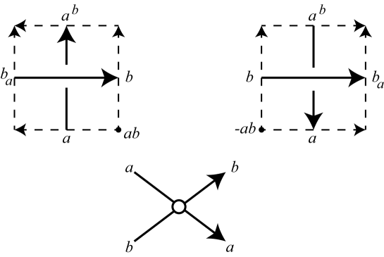
Figure 9: Conditions at a crossing

Fig. 10 below give pictorial evidence of the invariance under the Reidemeister moves. Full details can be obtained in [45]. Many examples of small size can be found in [6].

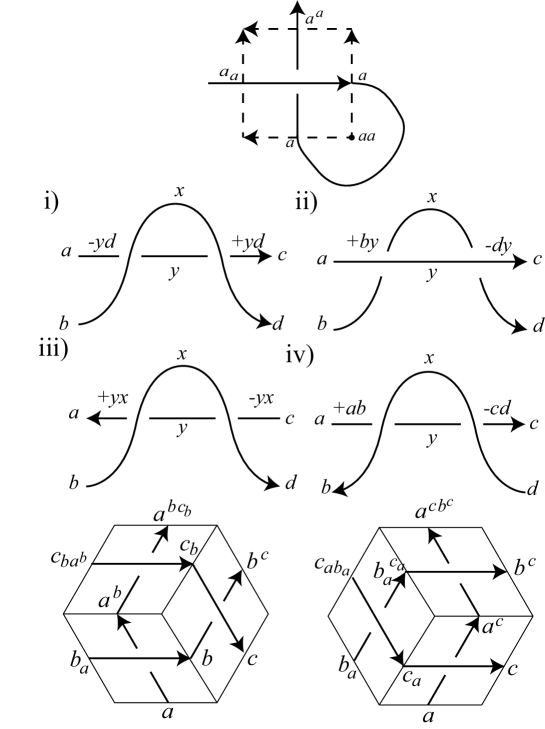
Figure 10: Invariance under the Reidemeister moves

On the other hand if we are looking for invariants of a doodle then we would not expect the Yang–Baxter condition to be satisfied.

Suppose $R$ is an associative ring with a multiplicative identity, 1. If the set of labels is an $R$-module, then the birack, biquandle, etc is called linear if there are are elements $A,\,B,\,C,\,D$ of $R$ such that the switch map is defined by the $2\times 2$ matrix

$$S=\left(\begin{array}[]{cc}A&B\\ C&D\end{array}\right).$$

There are many examples of linear biquandles with $R$ equal to the quaternions, see for example [14, 15, 44].

Affine biquandles, generalizing linear ones need to be investigated. One such is the Cheng labelling

$$S(x,y)=(y-1,x+1),$$

see [20].

6.2 Homology of biracks and biquandles

Let $X$ be the labels of a birack. A word $w=a_{1}\cdots a_{n}$ of length $n$ is called an $n$-cube. For example a 1-cube is a label, a 2-cube is a crossing and a 3-cube is a Reidemeister III move.

For each $n$-cube there are $2n$ faces of dimension $n-1$,

$$\partial_{i}^{-}(a_{1}\cdots a_{n})=a_{1}\cdots a_{i-1}a_{i+1}\cdots a_{n}$$

and

$$\partial_{i}^{+}(a_{1}\cdots a_{n})=(a_{1})^{a_{i}}\cdots(a_{i-1})^{a_{i}}(a_{i+1})_{a_{i}}\cdots(a_{n})_{a_{i}}\,\hbox{for}\,i=1,\ldots,n$$

A cubical cell complex, $\Gamma X$, can be defined in the usual way by identifying all the disjoint cubes having common faces. Properties of this complex can now be used to define knot invariants. For example the fundamental group has a presentation

$$\pi_{1}(\Gamma X)=\langle x,y\in X\mid xy_{x}=yx^{y}\rangle.$$

Let $C_{n}=C_{n}(\Gamma X)$ be the free abelian group with basis the $n$-cubes of $\Gamma X$. The homomorphism $\partial\colon C_{n}\to C_{n}$ is defined on cubes by

$$\partial=\sum_{i=1}^{n}(-1)^{i}(\partial_{i}^{-}-\partial_{i}^{+})$$

and extended linearly. The Yang–Baxter equations then imply that the composition

$$C_{n}\to C_{n-1}\to C_{n-2}$$

is zero, and so we have a chain complex. The homology of this chain complex $H_{*}(C)$ and the homology of any subchain complex is therefore an invariant.

One important example is the degenerate subchain. A cube, $a_{1}\cdots a_{n}$, is called degenerate if $a_{i}=a_{i+1}$, for some $i=1,\ldots,n-1$. If the birack is a biquandle, so $a^{a}=a_{a}$ for all $a$, then the degenerate cubes generate a subchain, $D_{*}$. The quotient $BQ_{*}=C_{*}/D_{*}$ defines the biquandle chain complex and the short exact sequence

$$0\to D_{*}\to C_{*}\to BQ_{*}\to 0$$

extends to a long exact homology sequence.

Another example is the double of a birack. Consider the set of pairs of pairs $X^{2}\times X^{2}$. Then $W\subset X^{2}\times X^{2}$ is the set of pairs of pairs defined by

$$W=\{ac,bc\mid a,b,c,\in X,c^{a}=c^{b}\}.$$

The doubled operations are

$$(ac)^{(bc)}=a^{b}c^{b},\,(bc)_{(ac)}=b_{a}c^{a}\,\hbox{and}\,G(ac,bc)=(b_{a}c^{a},a^{b}c^{a})$$

Doubling converts racks into biracks and quandles into biquandles.

The homology of the double of the 3-color quandle can be used to distinguish the right and left trefoils, see [45].

Much work has been done on the homology of racks and quandles, see [16, 50, 51, 52, 53]. However the homology of biracks and biquandles is little understood and needs investigating.

7 Graph-links

It turns out that some information about the knot can be obtained from a more combinatorial data: the intersection graph of a Gauss diagram. The intersection graph is a graph without loops and multiple edges, whose vertices are in one-to-one correspondence with chords of the Gauss diagram. Two vertices of the intersection graph are adjacent whenever the corresponding chords of the Gauss diagram are linked (or intersect each other when they are placed inside ), see Fig. 11. Each vertex of the intersection graph is endowed with the local writhe number of the corresponding crossing.

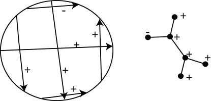
Figure 11: A Gauss diagram and its labeled intersection graph

However, sometimes a chord diagram can be obtained from the intersection graph in a non-unique way, and some graphs (shown in Fig. 12) cannot be represented by chord diagrams at all.

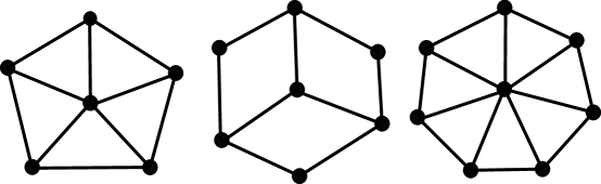
Figure 12: Non-realizable Bouchet graphs

Likewise virtual knots appear out of non-realizable chord diagram and thus generalize classical knots (which have realizable chord diagrams), graphs-links come out of intersection graphs: We may consider graphs which are realized by chord diagrams, and, in turn, by virtual links, and pass to arbitrary simple graphs which correspond to some mysterious objects generalizing links and virtual links.

Traldi and Zulli [213] constructed a self-contained theory of “non-realizable knots” (the theory of looped interlacement graphs) possessing lots of interesting knot theoretic properties by using Gauss diagrams. These objects are equivalence classes of (decorated) graphs modulo “Reidemeister moves”.

In [68] it was suggested another way of looking at knots and links and generalizing them (the theory of graph-links): whence a Gauss diagram corresponds to a transverse passage along a knot, one may consider a rotating circuit which never goes straight and always turns right or left at a classical crossing. One can also encode the type of smoothing (Kauffman’s $A$-smoothing or Kauffman’s $B$-smoothing) corresponding to the crossing where the circuit turns right or left and never goes straight, see Fig. 13. We note that chords of diagrams are naturally split into two sets: those corresponding to crossings where two opposite directions correspond to emanating edges with respect to the circuit and the other two correspond to incoming edges, and those where we have two consecutive (opposite) edges one of which is incoming and the other one is emanating.

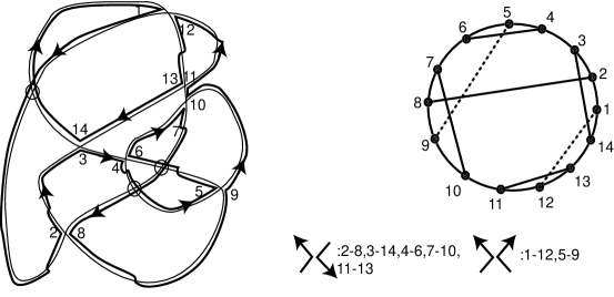
Figure 13: Rotating circuit shown by a thick line; chord diagram

After the two theories were constructed, some questions arose. It was shown that there are graphs not being Reidemeister equivalent (each theory has own Reidemeister moves) to an intersection graph of a virtual knot diagram [74, 176]. The equivalence of the two theories (the theory of looped interlacement graphs and the theory of graph-knots) was proved in [67]. Also, some invariants were constructed, see [68, 69, 71, 74, 193, 213].

8 A List of Problems

8.1 Problems in and related with virtual knot theory

Below, we present a list of research problems closely connected with virtual knot theory.

1. Recognising the Kishino Knot: There have been invented many ways to recognize the Kishino virtual knot (from the unknot): The $3$–strand Jones polynomial, i.e. the Jones polynomial of the $3$–strand cabling of the knot [132], the $\Xi$–polynomial, see [155], the quaternionic biquandle [5], and the surface bracket polynomial (Dye and Kauffman [35]). In [79] Kadokami proves the knot is non-trivial by examining the immersion class of a shadow curve in genus two. One can use the Manturov parity bracket [175, 176, 179] to show that essentially the flat Kishino diagram is its own invariant, exhibiting the non-triviality of this knot. See [94] for an exposition of this proof.

   Are we done with this knot? Perhaps not. Other proofs of its non-triviality may be illuminating. The fact that the Kishino diagram is non-trivial and yet a connected sum of trivial virtual knots suggests the question: Classify when a non-trivial virtual knot can be the connected sum of two trivial virtual knots. A key point here is that the connected sum of closed virtual knots is not well defined and hence the different choices give some interesting effects. With long virtual knots, the connected sum is ordered but well-defined, and the last question is closely related to the question of classifying the different long virtual knots whose closures are equivalent to the unknot.

2. Flat Virtuals: Flat virtual knots, also known as virtual strings [64, 214], are difficult to classify. Find new combinatorial invariants of flat virtual knots.

   We would like to know more about the flat biquandle algebra. This algebra is isomorphic to the Weyl algebra [55] and has no (non-trivial) finite dimensional representations. An example that goes beyond the usual restrictions is the (very simple) affine biquandle used in [106] to construct the Affine Index polynomial invariant of virtual knots. One can make small examples of the flat biquandle algebra, that detect some flat linking beyond mod $2$ linking numbers, but the absence of other finite dimensional representations presents a problem.

3. The Flat Hierarchy: The flat hierarchy is constructed for any ordinal $\alpha$. We label flat crossings with members of this ordinal. In a flat third Reidemeister move, a line with two $a$ labels can slide across a crossing labeled $b$ only if $a$ is greater than $b.$ This generalizes the usual to theory of flat virtual diagrams to a system with arbitrarily many different types of flat crossings. Classify the diagrams in this hierarchy. This concept is due to Kauffman (unpublished). A first step in working with the flat hierarchy can be found in [167].

4. Virtuals and the Theory of Doodles: Compare flat theories of virtual knots with theories of doodles. A doodle is represented by a flat diagram in the plane. Reidemeister moves of type I and II are allowed but not type III. So a triple point must not be allowed. Khovanov has associated a group to doodles [126]. Commutator identities can also be associated to a doodle. Cobordism of doodles is defined by an immersed surface without triple points. Cobordism classes represent elements of a free abelian group. There is undoubtably a rich seam of results which could be found by investigating doodles. For example there is no reason not to have virtual crossings as well as flat crossings. This would give doodles on a surface of higher genus, see [43, 54, 126].

5. Virtual Three Manifolds: There is a theory of virtual $3$–manifolds constructed as formal equivalence classes of virtual diagrams modulo generalized Kirby moves, see [36]. From this point of view, there are two equivalences for ordinary $3$–manifolds: homeomorphisms and virtual equivalence. Do these equivalences coincide? That is, given two ordinary three manifolds, presented by surgery on framed links $K$ and $L$, suppose that $K$ and $L$ are equivalent through the virtual Kirby calculus. Does this imply that they are equivalent through the classical Kirby calculus?

   What is a virtual $3$-manifold?: That is, give an interpretation of these equivalence classes in the domain of geometric topology.

   Construct another theory of virtual $3$–manifolds by performing surgery on links in thickened surfaces $S_{g}\times\mathbb{R}$ considered up to stabilization. Will this theory coincide to that proposed by Kauffman and Dye [36]?

6. Welded Knots: We would like to understand welded knots [198, 200]. It is well known [85, 190] that if we admit forbidden moves to the virtual link diagrams, each virtual knot can be transformed to the unknot. If we allow only one forbidden move (e.g. the upper one), then there are lots of different equivalence classes of knots. In fact the fundamental group and the quandle of the virtual diagram are invariant under the upper forbidden move. The resulting equivalence classes are called welded knots. Similarly, welded braids were studied in [48], and every welded knot is the closure of a welded braid. The question is to construct good invariants of welded knots and, if possible, to classify them. In [200] a mapping is constructed from welded knots to ambient isotopy classes of embeddings of tori (ribbon tori to be exact) in four dimensional space, and it is proved that this mapping is an isomorphism from the combinatorial fundamental group (in fact the quandle) of the welded knot to the fundamental group of the complement of the corresponding torus embedding in four-space. Is this Satoh mapping faithful from equivalence classes of welded knots (links) to ambient isotopy classes of ribbon torus embeddings in four-space?

   Another interesting question is the following: If a welded knot has trivial fundamental group, does this imply that the knot is trivial as a welded knot?

7. Long Knots and Long Flat Knots: Enlarge the long knot invariant structure proposed in [160]. Can one get new classical knot invariants from the approach in this paper? Bring together the ideas from [160] with the biquandle construction from [124] to obtain more powerful invariants of long knots. Long flat virtual knots can be studied via a powerful remark due to Turaev (in conversation) to the effect that one can associate to a given long flat virtual knot diagram $F$ a descending diagram $D(F)$ (by always going over before going under in resolving the flat (non-virtual) crossings in the diagram). The long virtual knot type of $D(F)$ is an invariant of the long flat knot $F.$ This means that one can apply any other invariant $I$ of virtual knots that one likes to $D(F)$ and $I[D(F)]$ will be an invariant of the long flat $F.$ It is quite interesting to do sample calculations of such invariants and this situation underlines the deeper problem of finding a full classification of long flat knots.

   Bartholomew, Fenn, S. Kamada and N. Kamada have applied quaternion invariants to long virtual knots, see [7].

   See also Sec. 8.4 for more questions about long virtual knots and long flat virtual knots.

8. Virtual Biquandle: Construct presentations of the virtual biquandle with the a linear (non-commutative) representation at classical crossings and some interesting structure at virtual crossings. A start has been made by Bartholomew and Fenn [6]. In this paper various biquandle decorations are made at classical and virtual crossings which were found by a computer search.

9. Virtual braids: Is there a birack such that its action on virtual braids is faithful?

   Is the invariant of virtual braids in [150], see also [3, 109, 162], faithful?

   The action defined by linear biquandles is not faithful. This almost certainly means that the corresponding linear invariants of virtual knots and links are not faithful [44] (see also [6]).

10. The Fundamental Biquandle: Does the fundamental biquandle, see [124] classify virtual links up to mirror images? (We know that the biquandle has the same value on the orientation reversed mirror image where the mirror stands perpendicular to the plane (see [64, 65]).

    Are there good examples of weak biquandles which are not strong? This problem is solved in [208].

    We would like to know more about the algebra with 2 generators $A,\,B$ and one relation $[B,(A-1)(A,B)]=0$ (see [14]). It is associated to the linear case.

11. Virtualization and Unit Jones Polynomial: Suppose the knot $K$ is classical and not trivial. Suppose that ${\tilde{K}}$ (obtained from $K$ by virtualizing a subset of its crossings) is not trivial and has a unit Jones polynomial, $V(\tilde{K})=1$. Is it possible that ${\tilde{K}}$ is classical (i.e. isotopic through virtual equivalence to a classical knot)?

    Suppose $K$ is a virtual knot diagram with unit Jones polynomial. Is $K$ equivalent to a classical diagram via virtual equivalence plus crossing virtualization? (Recall that by crossing virtualization, we mean flanking a classical crossing by two virtual crossings. This operation does not affect the value of the Jones polynomial.)

    Given two classical knots $K$ and $K^{\prime},$ if $K$ can be obtained from $K^{\prime}$ by a combination of crossing virtualization and virtual Reidemeister moves, then is $K$ classically equivalent to $K^{\prime}?$

    If the above two questions have affirmative answers, then the only classical knot with unit Jones polynomial is the unknot.

12. Virtual Quandle Homology: Study virtual quandle homology in analogy to quandle homology [17, 61].

13. Khovanov Homology: Construct a generalization of the Khovanov complex for the case of virtual knots that will work for arbitrary virtual diagrams. Investigate the Khovanov homology constructed in [162, 164]. The main construction in this approach uses an orientable atom condition to give a Khovanov homology over the integers for large classes of virtual links. The import of our question, is to investigate this structure and to possibly find a way to do Khovanov homology for all virtual knots over the ring of integers. Similar questions can be raised for the presently evolving new classes of Khovanov homology theories related to other quantum invariants (cf. [117, 118]).

    By a K-full virtual knot we mean a knot for which there exists a diagram such that the leading (the lowest, or both) term comes from the $B$-state. Analogously, one defines the Kho-full knot relative to the Khovanov invariant. Call such diagrams optimal diagrams. (It is easy to find knots which are neither K-full nor Kho-full.)

    Classify all K-full (Kho-full) knots.

    Are optimal diagrams always minimal with respect to the number of classical crossings?

    Classify all diagram moves that preserve optimality.

    Is it true that if a classical knot $K$ has minimal classical diagram with $n$ crossings then any virtual diagram of $K$ has at least $n$ classical crossings?

    Can any virtual knot have torsion in the $B$-state of the Khovanov homology (the genuine leading term of some diagram)? Here we use the formulation of Khovanov homology given in [162, 164].

    The behaviour of the lowest and the leading term of the Kauffman bracket for virtual knots was studied in [162] and [2] and [81].

14. Brauer algebra: The appropriate domain for the virtual recoupling theory is to place the Jones–Wenzl projectors in the Brauer algebra. That is, when we add virtual crossings to the Temperley–Lieb Algebra to obtain “Virtual Temperley–Lieb Algebra” the result is the Brauer algebra of all connections from $n$ points to $n$ points (see [114, 116]). What is the structure of the projectors in this context? Can a useful algebraic generalization of the classical recoupling theory be formulated?

15. Virtual Alternating Knots: Define and classify alternating virtual knots.

    Find an analogue of the Tait flyping conjecture and prove it. Compare [222].

    Classify all alternating weaves on surfaces (without stabilization).

16. Crossing Number: One of the most important problems in knot theory is the problem of finding the minimal crossing number for a given knot. It can be estimated by means of various invariants, the simplest one, perhaps, being the Kauffman bracket estimate:

    $$\mathrm{span}\langle K\rangle\leqslant 4n-4g,$$

    Here $\mathrm{span}$ stands for the difference between the leading degree and the lowest degree non-zero terms in the Laurent polynomial defined by the Kauffman bracket, $n$ is the crossing number, $g$ is the atom genus for the knot $K$ (also called the Turaev genus).

    In the case $g=0$, we get the celebrated Murasugi–Kauffman–Thistlethwaite’s theorem on minimality of alternating knot diagrams.

    Is there is a way to prove that the atom genus $g$ is minimal for a concrete knot diagram? Then this together with a sharp estimate for the span of the Kauffman bracket guarantees the minimality of the diagram.

    The estimate $4n-4g$ is exact for adequate diagrams (after Thistlethwaite). It is exact for many diagrams which are not adequate however: there are lots of minimal diagrams where the span of the Kauffman bracket “drops down”, for example, for torus $(p,q)$ knots for $p>q>2$.

    Why is the span of the Kauffman bracket smaller than expected for such classes of knots?

    One of possible explanations may be that the projection surface is wrongly chosen. For a torus knot, it is more convenient to consider it as being projected to the torus with no crossing points rather than to the plane with many crossing points. Thus the following problem arises: How do we use the Kauffman bracket, Thistlethwaite spanning tree, atoms and other invariants to get estimates for the number of crossings when projecting the knot diagram not to the plane but rather to some surfaces of higher genera?

    Certainly, when applying smoothing on the plane we get the final expansion of the Kauffman bracket as a linear combination of the bracket for the unknot; we shall get expression in terms of the bracket of some “basic” torus knots, which makes the problem harder.

    Can we get estimates from Thistlethwaite’s spanning tree and/or from the Khovanov homology?

    Which minimality theorems can be proved in this direction?

    Is it possible to get an estimate for the atom genus when the atom is considered not in the neighborhood of the plane but rather in a neighborhood of the surface the knot is projected to and the thickness of the Khovanov homology does not exceed $2+g$?

17. Crossing number problems: For each virtual link $L$, there are three crossing numbers: the minimal number $C$ of classical crossings, the minimal number $V$ of virtual crossings, and the minimal total number $T$ of crossings for representatives of $L$. There are also a number of unknotting numbers: The classical unknotting number is the number of crossing switches needed to unknot the knot (using any diagram for the knot). The virtual unknotting number is the number of crossings one needs to convert from classical to virtual (by direct flattening) in order to unknot the knot (using any virtual diagram for the knot). Very little is known. Find out more about the virtual unknotting number.

    What is the relationship between the least number of virtual crossings and the least genus in a surface representation of the virtual knot.

    Is it true that $T=V+L$?

    Is there any algorithm for finding $V$ for some class of virtual knots. For $T$, this is partially done for two classes of links: quasialternating and some other, see [152]. For classical links and alternating diagrams see [187, 189].

    Are there some (non–trivial) upper and lower bounds for $T,\,V,\,L$ coming from virtual knot polynomials (see [141])?

18. Wild Virtuals: Create the category of “wild virtual knots” and establish its axiomatics. In particular, one needs a theorem that states when a wild equivalence of tame virtual links implies a tame equivalence of these links.

19. Vassiliev Invariants: Understand the connection between virtual knot polynomials and the Vassiliev knot invariants of virtual knots (in Kauffman’s sense). Some of that was done in [60, 93, 166, 202].

    The key question about this collection of invariants is this: Does every Vassiliev invariant of finite type, for classical knots extend to an invariant of finite type for long virtual knots? Here we mean the problem in the sense of the formulation given in [60]. In [93] it was pointed out that there is a natural notion of Vassiliev invariants for virtual knots that has a different notion of finite type from that given in [60]. This alternate formulation needs further investigation.

20. Embeddings of Surfaces: Given a non-trivial virtual knot $K$. Prove that there exists a minimal realization of $K$ in $N=S_{g}\times I$ and an unknotted embedding of $N\subset\mathbb{R}^{3}$ such that the obtained classical knot in $\mathbb{R}^{3}$ is not trivial. (This problem is partially solved by Dye in [32].

21. Non-Commutativity and Long Knots: It is known that any classical long knot commutes with any long knot. This is definitely not the case in the virtual category, see paper by Kamadas, Fenn et al. However the commutativity of classical long knots may be incorporated into the commutativity of virtual knots if the following question is true. Is it true that if $K$ and $K^{\prime}$ are long knots and $K{\#}K^{\prime}$ is isotopic to $K^{\prime}{\#}K$ then there exists a virtual long knot $L$, classical long knots $Q,\,Q^{\prime}$, and non-negative integer numbers $m,n$ such that

    $$K=L^{m}{\#}Q,\quad K^{\prime}=L^{n}{\#}Q^{\prime},$$

    where by $L^{m}$ we mean the connected sum of $m$ copies of the same knot?

22. The Rack Space: The rack space was invented by Fenn, Rourke and Sanderson [42, 50, 51, 53]. The homology of the rack space has been considered by the above authors and Carter, Kamada, Saito [17]. For low dimensions, the homology has the following interesting interpretations. Two dimensional cycles are represented by virtual link diagrams consistently colored by the rack, and three dimensional cycles by the same but with the regions also colored. See the thesis of Greene [61]. So virtual links can give, in this way, information about classical knots! For the second homology of the dihedral rack, the results are given in Greene’s thesis. We now know that for a prime $p$ the third homology has a factor $\mathbb{Z}_{p}$, see [192].

    Another line of enquiry is to look at properties of the birack space [50] and associated homology.

    Beyond problem number 22 we list new problems that are added to this revised problem list.

23. Find new geometric/topological interpretations for the Jones polynomial and for Khovanov homology.

24. Let $VKT/Z$ denote virtual knot theory modulo $Z$-equivalence, as defined in the section above on virtual knot theory. Recall that two virtual diagrams that are $Z$-equivalent have the same Jones polynomial. It is known that classical knot theory embeds in virtual knot theory. Does classical knot theory embed in $VKT/Z?$ That is, suppose that $K$ and $K^{\prime}$ are classical knot diagrams, and suppose that $K$ and $K^{\prime}$ are equivalent using virtual moves and $Z$-moves. Does it follow that $K$ and $K^{\prime}$ are equivalent as classical knots?

25. Rotational virtual knot theory introduced in [93] is virtual knot theory without the first virtual move (thus one does not allow the addition or deletion of a virtual curl). This version of virtual knot theory is significant because all quantum link invariants originally defined for classical links extend to rotational virtual knot theory. This theory has begun to be explored [93, 108, 112] and deserves further exploration. We have formulated a version of the bracket polynomial for rotational virtuals that assigns variables according to the absolute value of the Whitney degree of state curves. See Figure 14 for examples of non-trivial rotational virtual links.

    

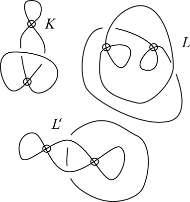
    Figure 14: Examples of non-trivial rotational links

    The rotational bracket can be generalised in the fashion of the Arrow Polynomial. Beyond this there are all the quantum link invariants and how they behave on rotational virtuals. We are in the process of writing a new paper on rotational virtual knot theory. A natural class of invariants for rotational virtuals arises as quantum invariants associated with finite dimensional quasi-triangular Hopf algebras. This harks back to an early project [121, 122, 123, 124] that needs further articulation. In that work with Radford we articulate invariants that immediately generalize to invariants of rotational virtual knots. These invariants are defined via integrals on finite dimensional Hopf algebras and should be studied for their own sake. We would also like to know about the possibility of categorification of finite dimensional Hopf algebras and, in particular, the meaning of categorifying a right integral.

26. The arrow polynomial generalizes to a more powerful invariant of virtual knots by defining a version of it for knots in specific thickened surfaces. The arrow polynomial for a knot in a thickened surface has state variables that take into account the isotopy class of the state curve and its arrow number as well. This gives a very strong invariant of knots in thickened surfaces and it can be applied to virtual knots by using a minimal surface representative for the virtual knot. Investigating this surface arrow invariant generalizes previous work on the surface bracket polynomial [35].

27. Study concordance and cobordism invariants of virtual knots. In particular, solve the question of virtual knots up to pass-equivalence [86] (taking a direct generalization of classical pass equivalence that gives the Arf invariant of knots). Understanding this specific problem will promote our understanding of concordance of virtual knots.

28. Biquandles: The first two problems are old chestnuts.

    Give a descriptive representation of the free biquandle.

    Give a topological explanation of the fundamental biquandle of a knot.

    Is there such a thing as a free partial biquandle: probably not.

29. Khovanov homology for virtual knots and links works directly with mod-$2$ coefficients. With mod-2 coefficients there are no technical difficulties associated with the fact that a virtual state curve can resmooth to a single curve. Over the integers, this is a problem that has to be dealt with. An integral Khovanov homology for virtual knots has been constructed by Manturov [169]. It is also the case that the work of Khovanov–Rozansky [130, 131] categorifiying infinitely many specializations of the Homflypt polynomial is an integral invariant for virtual knots. In principle, the Khovanov–Rozansky work solves the problem of integral Khovanov homology for virtuals, but to see this in terms of Khovanov’s original definition is a very good technical problem. Solve this problem to clarify the Manturov construction.

30. In [39, 80] we have studied a mod-2 categorification of the arrow polynomial and discovered many baffling examples of pairs of virtual knots that are discriminated by this link homology and not distinguished by Khovanov homology mod-2 or the arrow polynomial. We want to understand this new link homology and to that end will do more computations and will try to understand the structure of this homology theory for virtual links.

31. Make a systematic study of Vassiliev invariants for virtual knots and links. There is ongoing work on this problem.

32. Generalize virtual knot theory to virtual 2-spheres in 4-space.

33. Find a way to effectively compute the Kauffman–Radford–Hennings (KRH) invariants [121] for three-manifolds via right integrals on finite dimensional Hopf algebras [92]. Find a way to categorify the Kauffman–Radford–Hennings invariants for all finite dimensional quasitriangular Hopf algebras. The KRH invariants are actually invariants of rotational virtual links that are also, after normalization, invariant under the moves of the Kirby calculus. In this way, they give invariants of three manifolds and virtual three manifolds. The formulation of the KRH invariants in terms of integrals for finite dimensional Hopf algebras is very elegant, but computation is very difficult. Thus these invariants form a challenge for both virtual and classical knot theory. It is worth pointing out again, that the proper domain for all quantum link invariants is rotational virtual knot theory. Thus, this problem about the KRH invariants is a test case for the structure of quantum link invariants as a whole.

34. Create a combinatorial homotopy theory for Khovanov homology so that the Khovanov homology of a knot or link is equivalent to the homotopy type of an abstract complex (or category) associated with the knot of link. This problem is meant in the sprit of Bar-Natan’s reformulation of Khovanov homology as an abstract chain homotopy class of a categorical chain complex associated with the knot or link. Recent work of Lifshitz and Sarkar [142] goes very far in this direction. Of course we would like a deeper connection, and we would like to have the theory working for virtual knots and links.

35. In [90] we give a formula for the Kauffman polynomial, due to Jaeger, that expresses this invariant as a state sum over oriented, partially smoothed links associated with the given link. these states are evaluated by using the Homfly polynomial. Generalize the Jaeger point of view to obtain a categorification of the Kauffman polynomial by using chain complexes for these states that are derived from the Khovanov–Rozansky categorification of the Homflypt polynomial.

36. In [90, 95] we show how, by translating between knots and planar graphs (the checkerboard and medial constructions) one can associate a signed graph to a classical knot and that, with a choice of nodes and an interpretation of the signs as generalized electrical conductance, the conductance between two nodes of the graph is an invariant of isotopy of the knot restricted to move in the complement of these nodes. The moves on the graphs involve replacements of pedant loops and edges, series and parallel replacements and a star–triangle exchange move. These moves can be applied to abstract (possibly non-planar) graphs. As a result we obtain a generalization of knot theory (similar in spirit but quite different from virtual knot theory) by taking the electrical equivalence classes of signed graphs. Call this theory $EG_{\pm}.$ The conductance remains an invariant of these Electric–Knots and shows that the theory is highly non-trivial. This formulation of Electric Knots gives rise to many problems. Find new invariants of Graph-Knots. Note that if we take a planar immersion of a signed graph, then the induced cyclic orders of edges at the nodes of the planar embedding give a natural way (analogous to the medial graph) to associate a virtual knot diagram to the immersion. Explore this relationship of Electric Knots and virtual knots.

37. It has been pointed out that the chain complex for Knot Floer Homology [196] (categorifying the Alexander–Conway polynomial) is generated by the states described in Formal Knot Theory [86]. These states involve an assignment of pointers to each region of the diagram (with two adjacent regions omitted) such that each pointer marks a unique crossing in the diagram. The key problem about this complex is that while the chain groups are described via knot diagram combinatorics, the differential in the complex seem to require high dimensional contact geometry. Even though there is now a combinatorial definition of Knot Floer homology via arc diagrams, this is an unsatisfactory state of affairs. The problem is to find a combinatorial definition of the differential on the complex generated by the Formal Knot Theory states.

38. The Kauffman bracket polynomial of a virtual diagram can have the leading term, i.e., the term having the highest possible degree, equal to zero.

    Assume that we have a diagram for which the Kauffman bracket polynomial has the nonzero leading term. Classify moves (compositions of the generalized Reidemeister moves) establishing the equivalence in the class of diagrams with nonzero leading terms.

39. We still do not know whether the free knot whose Gauss diagram is a heptagon (i.e. consists of 7 chords each of which is linked with precisely two adjacent ones) is trivial.

40. Given a chord diagram $D$ we can construct the following formal chain complex. Formally speaking, this complex will look like a simplicial complex in all dimensions except zero, but one can get rid of this by using duality arguments.

    In dimension $-1$ there is just one chain denoted by $\emptyset$. In dimension $0$, the chains are in one-to-one correspondence with unoriented chords of the diagram $D$; in dimension $1$ the chains are in one-to-one correspondence with pairs of unlinked chords, for dimension $2$ we take triples of pairwise unlinked chords, etc.

    The differential acts on the $k$-tuple, $\{a_{1},\dots,a_{k}\}$ of pairwise unlinked chords to the $(k+1)$-tuple $\{a_{1},\dots,a_{k},a_{l}\}$ obtained by the addition of a chord unlinked with all the previous ones. The sign is taken in a standard way to make the complex well-defined with integral coefficients. Such a complex is naturally defined by the intersection graph of the chord diagram.

    • 8.1. Let the chord diagram consist of $2n$ chords, where the the following pairs of chords are linked: $(1,2)$, $(3,4)$, $(5,6),\dots,(2n-1,2n)$. Then the corresponding simplicial complex is the $(n-1)$-sphere (the $n$-th join of $S^{0}$.

    Can we get any other simplicial complexes this way other than just bouquets of spheres? An affirmative answer to this question may lead to some homological calculations which are very easy for computer implementation. This problem was motivated several years ago by an attempt to construct the spectrification of the Khovanov homology. It turns out that if some (virtual) knot in the $A$-state has exactly one circle then its Khovanov homology in the lowest quantum grading looks exactly as described above. Thus, this approach may be useful for understanding the Khovanov homology of chord diagrams as well as some other approaches to the Khovanov homology spectrification obtained by recent work with Lipshitz.

    On the other hand, this problem is motivated the construction of graph-link theory. Indeed, every triangulated manifold admits a shallow triangulation such that together with any 1-frame of a $k$-simplex, it contains the whole simplex.

    Considering the one-dimensional frame of such a triangulation as the non-intersection graph of some chord diagrams, we get exactly the chord diagram, whose lower term Khovanov homology looks as described above. The problem is that not every graph is an intersection graph (neither any graph is a non-intersection graph) of any chord diagram. This leads to the graph-link theory for which all possible manifolds appear in the lower degree homology theory. This leads to some lower homotopy of graph links. The next problem can be formulated as follows.

    Given two diagrams of (virtual) knots or links with exactly one circle in the $A$-state. Which combinations of Reidemeister moves on the diagrams have to be be considered in such a way that whenever two diagrams generate equivalent knots, there exists a chain of moves from one diagram to the other with all intermediate diagrams having single-circle $A$-state and such that chord diagram homology (and homotopy) corresponding to those intermediate diagrams do not change under such moves?

    It is worth comparing these thoughts with the recent work of Lipschitz on the spectrification of Khovanov homology. Possibly, the Bloom–Nikonov [11, 193, 194] approach to Khovanov homology [195, 196] can be used here.

41. Which quantum invariants extend to virtual knots themselves without restrictions? Certainly, there are such ones, e.g., the Kauffman bracket and the Jones polynomial.

42. One can consider braids with even numbers of strands. Markov’s moves change the parity of the number of strands. Can one reformulate Markov’s theorem in such a way that only braids with even numbers of strands take part in this formulation?

43. In his wonderful paper [199], which firstly had the title “Knot Floer Homotopy”, Sarkar constructs a cell complex. The homology of this complex coincides with the Floer homology. In this work the following main ingredients are used: Manolescu–Ozsváth–Sarkar–Szabó–Thurston approach allowing one to define Heegaard–Floer homology by using grid diagrams and shellability. Roughly speaking, if complexes look like order complexes, then they can be replaced with cell (simplicial) complexes homotopically equivalent to them.

    Try to do the same things for Khovanov homology. In the initial Khovanov definition this problem seems to be very difficult, since the set of chains and states can hard be ordered. However, taking into account Bloom’s construction [11] this problem looks more optimistic.

44. A complete invariant is used for proving that one theory is a part of another theory. For example, the fact that the set of classical knots is a part of the set of virtual knots, is true for the same reason as a quandle with peripheral structure can be extended from classical knots into virtual knots. Analogous statements can be done for classical and virtual braids (the extension of Hurwitz’s action).

    So, we get an actual problem: how can one construct a complete invariant for virtual knots?

45. To prove that the invariant $\mathcal{F}$ constructed by V. O. Manturov for virtual braids, is complete for virtual braids with more than two strands.

46. In [184] it was showed how one could determine non-invertibility of long virtual knots and non-commutativity of long virtual knots. This method used two type crossings: an early undercrossing and an early overcrossing. Further, for two types we have different operations, these operations are similar but not coincide (these operations are related to quandles). Regretfully, this method gives nearly nothing for classical knots. But it is universal: instead of the construction of quandle with two operations one can consider other ways of constructing knot invariants. In these ways we partition the set of crossings into two subsets, and for each subset we use an operation. Moreover, two operations are different enough to determine non-invertibility, and in the same time are similar to give an invariant structure. In the level of the Kauffman bracket polynomial this construction does not work. We get two problems.

    1. Try to do the same for other objects than quandles, for example: nonlinear quandles, quandles with rings having non-unique decomposition of multiples.

    2. Try to apply it on a “categorified level”: use the usual chain space for Khovanov homology and in it two different differentials but commute with each other (these differentials correspond to circle and star operations). These two different differentials could arise from usual and odd Khovanov homologies in the case when we have an identification (but maybe not canonical) between chain spaces of these complexes. It is expected that these invariants could recognize non-invertibility of knots.

47. It is well known that flat virtual knots are easily algorithmically recognizable, see [63]. The absence of a geometric approach to the definition of free knots leads to the lack of the methods for solving the following three problems.

    1. Is it true that (any) connected sum of free knots is trivial?

    2. Are free knots algorithmically recognizable?

    3. Prove that free knots do not commute in the general case.

    In the first case we suggest that the answer is affirmative, and the proof should be a certain modification of the analogous proof for virtual knots (see, e.g., [137])

    In the second case we suggest that the answer is negative. It seems to us that free knots are a very complicated object, where one can construct models for many logical constructions.

    The third problem seems to be solvable by using (and, possibly, extending) standard methods in the free knot theory.

48. The functorial mapping was constructed, by means of it we constructed the map from the set of virtual knots to the set of virtual knots with orientable atoms.

    Can one construct an analogous map which projects the set of virtual knots to the set of classical knots? For example, one can try to find an index by using characteristic classes. Here only one condition which arises under the third Reidemeister move should hold.

    Note that in the case of homologically trivial knots we can consider a two-branched covering like a projection.

49. Turaev constructed the map from the set of long flat knots to the set of long virtual knots. Can one construct any map from the set of long free knots to the set of long virtual knots? This question can be extended and one can try to construct any map which “enlarge” the structure.

50. The problem about cobordisms in sections: Let us have a free knot and its cobordism. Construct a parity on the given free knot, which is defined by using only this cobordism and respect only moves inside this cobordism.

51. Prove or disprove the conjecture about the non-uniqueness of minimal representative of a free link, i.e. there exists a free link having several minimal representatives.

52. If $X$ is the free rack, is $\Gamma X$ a cat(0) space? A positive answer would imply that all its higher homotopy groups are trivial.

53. Is there any algorithm for recognition whether two graph-links are equivalent or not? Our conjecture is “no”. The idea behind that is that graph-links are complicated enough, and possibly, they contain sufficiently many degrees of freedom to include something like Turing machines. All mathematics is roughly split into the recognizable one (low-dimensional topology, hyperbolic groups, decidability) and the non-recognizable one (topology of dimension $4$ and higher, arbitrary finitely presentable groups, Turing machines etc). The usual argument for undecidability for finitely presented group allows one to construct some universal (semi)groups which includes the apparatus of the Turing machines. We think that graph-links are enough complicated to include similar things: they contain arbitrary graphs, and Reidemeister moves, in principle, could play the role of “rules for formal languages” or “group relations”. It seems unlikely that Reidemeister moves collapse graph-links to anything simple enough because of the parity considerations: there are “irreducibly odd” graph-links which are stable in the sense that every equivalent graph contains the initial graph as a subgraph.

54. Can one construct a projection from the set of graph-links to the set of realizable graph-links?

55. Construct a parity on graph-links by using Bouchet’s criterion about the realizability of a graph. Try to find a parity which is responsible for the cyclically 6-edge connection, see [12].

56. Construct generalizations of the Frobenius extension [128] and the Rasmussen for “rigid” graph-links with orientable atoms.

57. Is it true that two equivalent realizable graph-links are equivalent in the class of realizable graph-links? If it is not true, then construct an example.

58. Construct a group for graph-links which is analogous to the group from [184, Subsection 8.9].

59. Construct “graph-braids”.

60. Problems on Free Knot Cobordism: The methods used for proving the fact that the invariant $L$ [73] gives an obstruction to the sliceness are not immediately generalized for obtaining lower estimates on the slice genus of free knots. Two reasons are as follows. First, when we define a parity and justified parity for double lines on $\mathcal{D}$, we chose an arbitrary curve connecting the two preimages of the point on the double curve. We assert that any two curves connecting these two preimages (and behaving correctly in neighborhoods of the ends) are homotopic. It is true in the case of cobordism of genus zero, but in the case of a surface of an arbitrary genus $h$ it is, indeed, not true.

    Thus, in order to define a parity for double lines we have to impose some restrictions on the spanning surface: we have to require that the cohomology class dual to the graph $\Psi$ was $\mathbb{Z}_{2}$–homologically trivial. The significance of the property for even-valent graphs to be $\mathbb{Z}_{2}$–homologically trivial is closely connected with atoms (for details see Sec. 4 and [176]).

    Another problem is that the Reeb graph of an arbitrary Morse function (not necessarily corresponding to the disc) is not necessarily a disc. Consider Fig. 15.

    

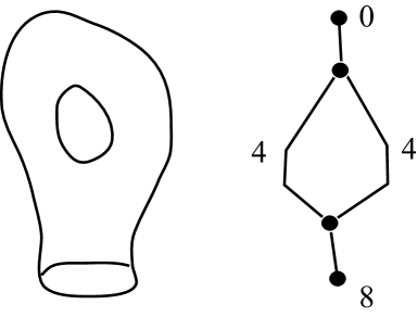
    Figure 15: The Reeb graph corresponding a cobordism of genus one

    Thus, starting from a free knot $K$ for which, we say, $L(K)=8$, we (in principle) can turn it by a Morse bifurcation into free two-component link consisting of two free knots $K_{1}$ and $K_{2}$, for which $L(K_{i})=4$, and then by another Morse bifurcation we can reconstruct this trivial link into the unknot. The invariant $L$ is not an obstruction to this, since the sum of $4$ and $-4$ is zero.

    In some cases we can overcome these two difficulties for cobordisms (of arbitrary genus).

    Let $\mathcal{D}_{g}$ be a surface with boundary $S^{1}$. Obviously, the collection of double lines of $\mathcal{D}_{g}$ defines a relative $\mathbb{Z}_{2}$–homology class $\kappa\in H_{1}(\mathcal{D}_{g},S^{1};\mathbb{Z}_{2})$. This homology class is an obstruction for the surface to be checkerboard-colorable; also, this is an obstruction for well-definedness of even/odd double lines.

    Namely, if we look at the definition of an even/odd double line: we see that there is an ambiguity in the choice of path connecting two preimages of a generic point on the double line. For the case of a disc cobordism, the parity of double lines is well defined, because all such curves are homotopic. For $\mathcal{D}_{g}$ the unique obstruction to this well-definedness is the class $\kappa$.

    We call a cobordism of genus $g$ checkerboard (or atomic) if the corresponding class $\kappa$ vanishes.

    The next task (after detecting which $1$-stratum is even and which one is odd) is to distinguish between $b$ and $b^{\prime}$. To this end, one should do the same for preimages of points lying on odd $1$-strata, connect them by a generic curve, and count the intersection with even double lines. So, we see that the only obstruction is the relative $\mathbb{Z}_{2}$–homology class $\kappa^{\prime}\in H_{1}(\mathcal{D}_{g},S^{1};\mathbb{Z}_{2})$ generated by even double lines.

    We say that a checkerboard cobordism is $2$-atomic if $\kappa^{\prime}$ vanishes.

    The following theorem holds.

    Theorem 8.1 (see [178]).

    Assume for a $1$-component framed $4$-graph $K$ we have $L(K)\neq 0$. Then there is no $2$-atomic cobordism spanning the knot $K$ of any genus.

    In the papers [143, 144] the fourth author constructed a strengthening $G_{m}$ of the group $G$ given in the present work (in the notation [143] our group $G$ is $G_{1}$) and the invariants of free knots with values in the classes of conjugate elements from $G_{m}$. The idea is as follows. Even chords are further partitioned into chords of different types, it leads to more accurate definition of generators and relations in the group; these constructions are closely connected with iterated parities and the map deleting odd crossings. It seems that all invariants related to the groups $G_{m}$ also give an obstruction to the sliceness of a knot. Moreover, in the paper [183] the author constructed invariants of virtual knots in which the over/undercrossing structure was taken into account besides the parity of chords. We devote a separate paper to the investigation of a connection of these invariants with cobordisms.

8.2 Problems on virtual knot cobordism

The material in this section will appear in [34, 108] and there have been studies of virtual knot cobordism at the free knot level by Manturov [178, 179, 181].

• 8.1. Two oriented knots or links $K$ and $K^{\prime}$ are virtually cobordant if one may be obtained from the other by a sequence of virtual isotopies (Reidemeister moves plus detour moves) plus births, deaths and oriented saddle points, as illustrated in Fig. 16. A birth is the introduction into the diagram of an isolated unknotted circle. A death is the removal from the diagram of an isolated unknotted circle. A saddle point move results from bringing oppositely oriented arcs into proximity and resmoothing the resulting site to obtain two new oppositely oriented arcs. See the figure for an illustration of the process. Fig. 16 also illustrates the schema of surfaces that are generated by cobordism process. These are abstract surfaces with well defined genus in terms of the sequence of steps in the cobordism. In the figure we illustrate two examples of genus zero, and one example of genus $1$. We say that a cobordism has genus $g$ if its schema has that genus. Two knots are cocordant if there is a cobordism of genus zero connecting them. A virtual knot is said to be a slice knot if it is virtually concordant to the unknot, or equivalently if it is virtually concordant to the empty knot (The unknot is concordant to the empty knot via one death.). This definition is based on the analogy of virtual knot theory and classical knot theory. It should be compared with [216] in the category of virtual strings.

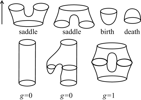
Figure 16: Saddles, births and deaths

In Fig. 17 we illustrate the virtual stevedore’s knot, VS and show that it is a slice knot in the sense of the above definition. We will use this example to illustrate our theory of virtual knot cobordism, and the questions that we are investigating. We define a virtual knot to be a ribbon virtual knot if it is slice via only deaths and saddle point transformations. We do not know at this point whether there are virtual slice knots that are not ribbon. With the same definitions restricted to classical knots, this is a long-standing open problem for classical knot theory.

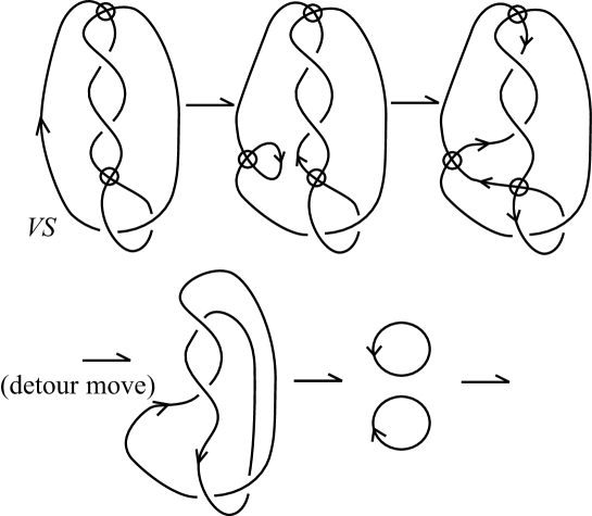
Figure 17: Virtual stevedore is slice

We first point out that the virtual stevedore ($VS$) is an example that illustrates the viability of this theory. We can prove that $VS$ is not classical by showing that it is represented on a surface of genus one and no smaller. The technique for this is to use the bracket expansion on a toral representative of $VS$ and examine the structure of the state loops on that surface (see Fig. 18). Note that in this figure the virtual crossings correspond to parts of the diagram that loop around the torus, and do not weave on the surface of the torus. An analysis of the homology classes of the state loops shows that the knot cannot be isotoped off the handle structure of the torus.

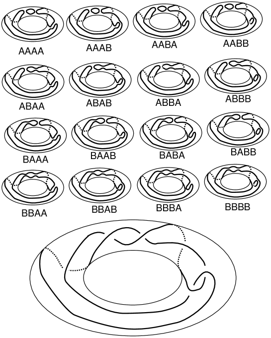
Figure 18: Virtual stevedore is not classical

Next we examine the bracket polynomial of the virtual stevedore, and show as in Fig. 19 that it has the same bracket polynomial as the classical figure eight knot. The technique for showing this is to use the basic bracket identity for a crossing flanked by virtual crossings as discussed in the previous section. This calculation shows that $VS$ is not a connected sum of two virtual knots. Thus we know that $VS$ is a non-trivial example of a virtual slice knot, an example that constitutes proof in principle that this project is viable. We will face the problem of the classification of virtual knots up to concordance.

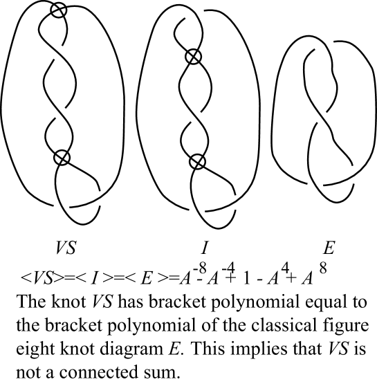
Figure 19: Bracket polynomial of the virtual stevedore

8.2.1 Virtual surfaces in four-space

We now define a theory of virtual surfaces in four-space that is given by moves on planar diagrams. One of the projects of this proposal is to investigate the relationships between this diagrammatic definition and more geometric approaches to virtual $2$-knots due to Jonathan Schneider and to Takeda [210] (see also [209]). One should also compare with the relationships to surfaces in four space for welded knots due to Satoh [200]. We make diagrammatic definitions as follows: We use middle level markers as indicated in Fig. 20 to encode two directions of smoothing a marked crossing in a planar diagram. The classical interpretation of such a marker is that it represents a cobordism through a saddle point at the middle level ($t=0$ in the figure) where the forms of smoothing above ($t=1$) and below ($t=-1$) are shown via the conventions in the figure. A diagram with markers can then be interpreted as two cobordisms attached at the middle. One cobordism goes downward to a collection of possibly linked and knotted loops, the other goes upward to another collection of linked and knotted loops. We will refer to these as the up-cobordism and the down-cobordism. A marked diagram is said to be excellent if both the up and the down cobordisms end in collections of unlinked circles that can be capped off with births (from the bottom) and deaths (at the top). The resulting schema is then a two-sphere and classically represents a two-sphere in four space. We take exactly this definition for a virtual two-sphere where it is understood that the ends of the two cobordisms will be trivial virtual links.

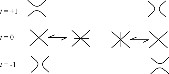
Figure 20: Middle level markers

Just as in classical theory, if a virtual knot is slice, then we can make a virtual two-sphere from it by using the same cobordism both up and down. Births for the original cobordism have to be represented directly in the middle level. The slicing example for $VS$, the virtual stevedore’s knot, can be made into a two-sphere this way. We show the middle level diagram for this sphere, called $S$ in Fig. 21. In this same figure, we show another middle level diagram for a virtual two-sphere $S^{\prime}.$ In this case we have used the fact (the reader can verify) that $VS$ can be sliced from its right-hand side. The sphere $S^{\prime}$ is obtained by slicing upward from the left and downward from the right.

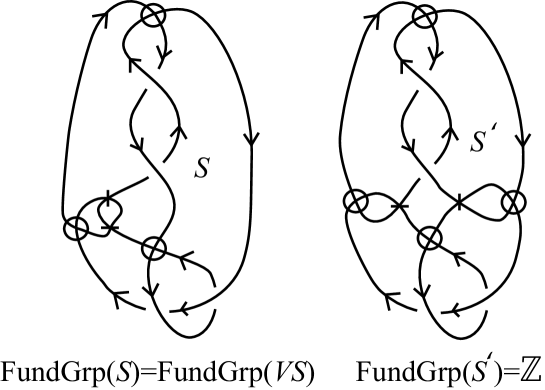
Figure 21: Two two-spheres

We give moves on the middle level diagrams to define isotopy of the virtual two-spheres obtained from the middle level diagrams. The moves are indicated in Fig. 22. They are a virtual generalization of the Yoshikawa moves that have been studied [140, 209] for isotopies of the classical middle level formulations. Thus we say the two two-spheres are isotopic if one can be obtained from the other via these Generalized Yoshikawa moves. In particular, the fundamental group of the two-sphere,defined by adding relations at saddle points exactly as in the classical case (but from the virtual knot theoretic fundamental group) is an isotopy invariant. For example, in Fig. 23 we calculate the fundamental group of $VS$ and find that, in it the arcs whose elements must be identified to obtain the fundamental group of the sphere $S$ of Fig. 21 are already identified in the fundamental group of $VS$. Thus we find that the sphere $S$ is knotted since it has the same non-trivial fundamental group as $VS.$ On the other hand, it is not hard to see that the fundamental group of the sphere $S^{\prime}$ is isomorphic to the integers. At this writing we do not know if this sphere is virtually unknotted.

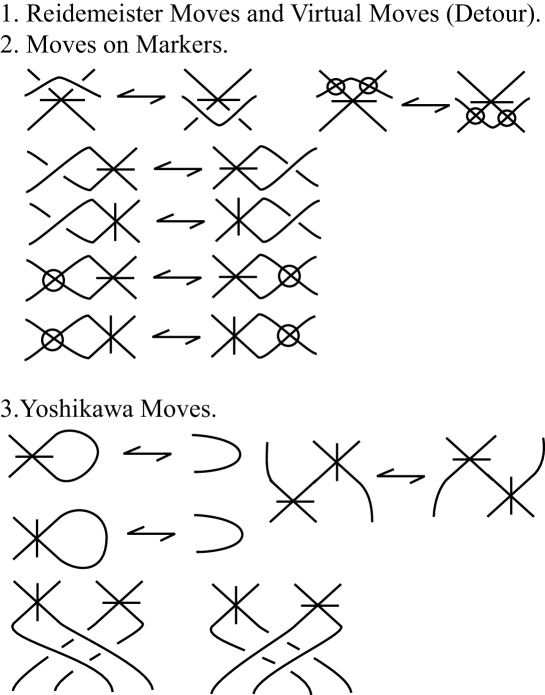
Figure 22: Middle level moves

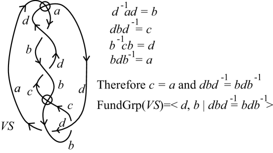
Figure 23: Fundamental group of $VS$

The generalized Yoshikawa moves present a useful first formulation for a theory of virtual surfaces. One of the advantages of this approach is that we can adapt the generalization of the bracket polyomial of Sang Youl Lee [140] to obtain a bracket invariant for virtual two-spheres. This will be an important subject of investigation for this proposal. We want to know how this diagrammatic formulation is related to immersions of surfaces in four space that could represent virtual two-knots. In this case the levels (movie of a cobordism) description that we have adopted gives such an immersion, and one can begin the investigation at that point. For these reasons, we believe that this formulation of virtual cobordism and virtual surfaces will be very fruitful and lead to many new results.

8.2.2 Virtual Khovanov homology

Khovanov homology [127] (see also [8, 10, 104, 105, 137, 139, 188, 217, 219]) for classical knots works, with mod-$2$ coefficients, for virtual knots. It has been generalized by Manturov [169, 184] for a homology theory with integer coefficients. We have a new formulation of Manturov’s construction that simplifies some of the choices in constructing the chain complex. We hope to see new results from this technology. In particular we are examining the structure of the Rasmussen invariant [197] with an eye to generalizing it in this framework. Using the notions of cobordism given here, we can define the virtual four genus of a virtual knot as the least cobordism genus that it can attain. Thus slice knots have genus zero and others will have higher genus in this sense. The Rasmussen invariant gives a lower bound on the 4-ball genus of classical knots. One can and we are investigating a similar lower bound for the virtual four genus.

8.2.3 Band-passing and other problems

The Arf invariant of a classical knot can be interpreted as the pass-class of the knot, where two knots are pass equivalent [88] if one can be obtained from the other by ambient isotopy combined with switching pairs of oppositely oriented pairs of parallel strands. The pass-class is a concordance invariant of classical knots and closely related to the Alexander polynomial. We would like to determine the pass-classes of virtual knots. This problem appears difficult at this time due the lack of invariants of the passing operation. We can obtain partial results by restricting passing to only odd crossings (then the Manturov parity bracket described in this proposal is an invariant of odd passing) but this is only a step on the way to understanding the pass equivalence relation for virtual knots. We expect that understanding this relation will shed light on problems of knot concordance.

We cannot resist ending this collection of problems with a very classical problem in skein theory. It is well-known that the Alexander polynomial of a slice knot is of the form $f(t)f(1/t)$ up to powers of $t$ and a sign. The problem is to give a proof of this result using only Conway skein theory. This problem has resisted us for a long time, and its resolution would surely shed light on problems of knot cobordism classical and virtual.

8.2.4 Questions from Micah W. Chrisman

In recent talks, Kauffman has defined notions of cobordism, concordance, slice, and ribbon for virtual knots. Turaev [215] has introduced a notion of cobordism for knots in thickened surfaces. A knot in $\mathbb{R}^{2}\times\mathbb{R}$ that is slice in the classical is slice in both the notions of Turaev and Kauffman. In [215], it is observed that it is unknown whether the converse is true

1. Are there any classical knots that are non-slice in the classical sense but are slice in the the sense of Kauffman (when considered as virtual knots) or Turaev (when considered as a knot in a thickened surface)?

2. If a knot in the thickened surface is slice in the sense of Turaev, does it necessarily stabilize to a virtual knot that is slice in the sense of Kauffman?

8.3 Questions from V. Bardakov

The virtual braid group $VB_{n}$ is defined by the generators $\sigma_{1},\,\sigma_{2},\ldots,\sigma_{n-1}$ which are generate the braid group $B_{n}$ and the generators $\rho_{1},\,\rho_{2},\ldots,\rho_{n-1}$ which are generate the symmetric group $S_{n}$ also the following mixed relations hold

$$\sigma_{i}\rho_{i+1}\rho_{i}=\rho_{i+1}\rho_{i}\sigma_{i+1},\leavevmode\nobreak\ \leavevmode\nobreak\ \leavevmode\nobreak\ i=1,2,\ldots,n-2;$$

$$\sigma_{i}\rho_{j}=\rho_{j}\sigma_{i},\leavevmode\nobreak\ \leavevmode\nobreak\ \leavevmode\nobreak\ |i-j|>1.$$

1. The group $G$ is called linear if there is an embedding of $G$ into the linear group $\mathrm{GL}_{m}(k)$ for some natural $m$ and a field $k$.

   Is it true that $VB_{n}$ is linear for all $n>3$?

   It is true for $n=3$ (unpublished result of V. Bardakov and P. Bellingeri).

2. Let $F_{n+1}=\langle x_{1},x_{2},\ldots,x_{n},y\rangle$ be a free group of rank $n+1$. There is a representation $\rho\colon VB_{n}\to\mathrm{Aut}(F_{n+1})$:

   $$\sigma_{i}:\left\{\begin{array}[]{ll}x_{i}\longmapsto x_{i}x_{i+1}x_{i}^{-1},&\\ x_{i+1}\longmapsto x_{i},&\\ x_{k}\longmapsto x_{k},&\\ y\longmapsto y,&\\ \end{array}\right.\leavevmode\nobreak\ \leavevmode\nobreak\ \leavevmode\nobreak\ \leavevmode\nobreak\ \rho_{i}:\left\{\begin{array}[]{ll}x_{i}\longmapsto yx_{i+1}y^{-1},&\\ x_{i+1}\longmapsto y^{-1}x_{i}y,&\\ x_{k}\longmapsto x_{k},&\\ y\longmapsto y,&\\ \end{array}\right.$$

   where $k\neq i,\,i+1$. This representation is an extension of the Artin representation $\rho_{A}\colon B_{n}\to\mathrm{Aut}(F_{n})$ which is faithful, i.e. $\mathrm{ker}(\rho_{A})=1$.

   Is the representation $\rho$ faithful for all $n>2$?

3. The virtual knot theory is a subtheory of the welded knot theory? The welded braid group $WB_{n}$ is the quotient of the virtual braid group $VB_{n}$ by the relations

   $$\rho_{i}\sigma_{i+1}\sigma_{i}=\sigma_{i+1}\sigma_{i}\rho_{i+1},\leavevmode\nobreak\ \leavevmode\nobreak\ \leavevmode\nobreak\ i=1,2,\ldots,n-2.$$

   The group $WB_{n}$ is a subgroup of $\mathrm{Aut}(F_{n})$ and the representation $\rho_{A}$ defined above is in fact the representation of $VB_{n}$ into $WB_{n+1}$. In the virtual knot theory as in the welded knot theory we have analogs of the Alexander theorem: every link is equivalent to the closure of some braid.

   Are there some non-equivalent virtual links $L_{v}$ and $L_{v}^{\prime}$ that are the closures of the virtual braids: $L_{v}=\widehat{\beta_{v}}$ and $L_{v}^{\prime}=\widehat{\beta_{v}^{\prime}}$ for some $\beta_{v}\in VB_{n}$, $\beta_{v}^{\prime}\in VB_{m}$ such that the welded links $\widehat{\rho_{A}(\beta_{v}})$ $\widehat{\rho_{A}(\beta_{v}^{\prime}})$ are equivalent as welded links?

4. The flat virtual braid group $FVB_{n}$ is the quotient of the virtual braid group $VB_{n}$ by the relations

   $$\sigma_{i}^{2}=1,\leavevmode\nobreak\ \leavevmode\nobreak\ \leavevmode\nobreak\ i=1,2,\ldots,n-1.$$

   Is there a representation $\varphi\colon FVB_{n}\to\mathrm{Aut}(F_{m})$ for some $m$ such that in the image the forbidden relations

   $$\varphi(\rho_{i})\varphi(\sigma_{i+1})\varphi(\sigma_{i})=\varphi(\sigma_{i+1})\varphi(\sigma_{i})\varphi(\rho_{i+1}),\leavevmode\nobreak\ \leavevmode\nobreak\ \leavevmode\nobreak\ i=1,2,\ldots,n-2$$

   do not hold?

8.4 Questions from Karene Chu

1. Long Virtual Knots and Long Flat Virtual Knots: Even though (round) flat virtual knots are not well understood, it turns out long flat virtual knots can be completely classified. They are in bijection with the subset of all signed permutations of in which consecutive pairs are not sent to oppositely signed consecutive pairs [28]. For example, $1\mapsto(3,+)$, $2\mapsto(2,-)$, $3\mapsto(4,-)$, $4\mapsto(1,+)$ is excluded since the pair $(1,2)$ is mapped to the oppositely signed consecutive pair $((3,+),(2,-))$. This classification is an invariant on long virtual knots; in particular, it gives necessary conditions for a long virtual which is classical, and can distinguish the long Kishino knots from the unknot. How can we use this invariant to understand long free knots, or round flat virtual knots, both of which are quotients of long flat virtual knots?

   Long flat virtual knots are also equivalent to long descending virtual knots by sending each flat real crossing to a descending crossing. The long descending virtual knots all have cyclic fundamental groups. What are the characteristics of the knot polynomials on this subset of long virtual knots?

   In fact, flat virtual pure tangles, whose skeletons are labelled long strands, are also completely classified by the same approach. There is a well-defined map from flat virtual braids in to flat virtual pure tangles simply by interpreting the braid diagram as a tangle diagram. It was pointed out in Chu’s talk that if this map is injective, then this classification also gives normal forms for flat virtual braids. How to show that this map is injective?

2. Virtual braids and flat virtual braids and braid-like virtual knots: The classifying spaces for both the flat virtual braid group and the virtual braid group have been constructed in [4]. (In this paper the flat virtual and virtual braid groups are called the triangular and quasi-triangular groups respectively.) Indeed, the classifying space of the flat virtual braid group is a beautiful space which is the quotient of the permutohedron by a natural action of the symmetric group. But from another perspective, what are the characterizations of the flat virtual or virtual braids in terms of embeddings into surfaces or thickened surfaces with boundary modulo stabilization?

   The equivalence generated by the subset of “braid-like” Reidemeister II and III moves, defined in Fig. 24, is a proper subset of the equivalence generated by the set of all Reidemeister II and III moves. “Braid-like” or “acyclic” Reidemeister II and III moves, shown as $R2b$ and $R3b$, are moves whose diagrams contain no oriented cycles (with the crossing as vertices). Cyclic moves, $R2c$ and $R3c$, contain oriented cycles. The set of virtual knot diagrams modulo only braid-like Reidemeister moves are called braid-like virtual knots by Bar-Natan. One can construct quantum invariants of these simply by “attaching R-matrices of quantum groups to the real crossings” and ignoring cups and caps, unlike for classical knots (see [129]). What are braid-like virtual knots topologically?

3. Welded braids and Knots: The welded braid group is the basis-conjugating subgroup of the automorphism group of the free group and includes the classical braids. It has been completely classified with normal forms in [62]. We can ask which properties of the classical braid group are also possessed by the welded braid group, e.g., automaticity, orderability, linearity?

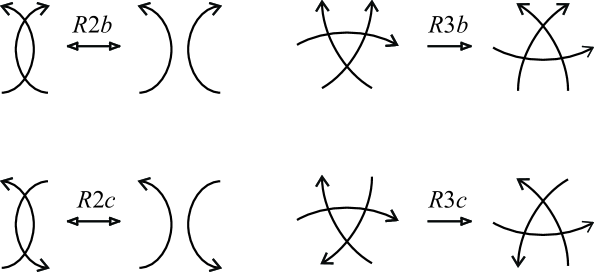
Figure 24: $R2b$, $R2c$, $R3b$ and $R3c$ moves

8.5 Questions from Micah W. Chrisman

8.5.1 Finite-type invariants

Finite-type invariants of classical knots can be understood through the Kontsevich integral, configuration space integrals, and combinatorial formulae (see [98]). There is no corresponding general theory for Vassiliev invariants of virtual knots.

There are two notions of finite-type invariants of virtual knots: the Goussarov–Polyak–Viro finite-type invariants and the Vassiliev finite-type invariants (introduced to the virtual knot case by Kauffman). There is a universal finite-type invariant for the GPV finite-type invariants by way of the Polyak algebra. On the other hand, there is no known universal finite-type invariant for Vassiliev finite-type invariants.

In fact, the two types are quite different. The GPV finite-type invariants are finitely-generated at every order. The Vassiliev finite-type invariants are however infinitely generated. There is even an infinite number of different extensions of the Conway polynomial to virtual knots, all satisfying the same skein relation and whose coefficients give an infinite family of finite-type invariants of every order [21]. Also, there are obstructions for when a Vassiliev finite-type invariant can be represented by an arrow diagram formula in the sense of Goussarov–Polyak–Viro. For example, an integer valued Vassiliev invariant which is invariant under the virtualization move cannot be a GPV finite-type invariant [23].

1. Classify all obstructions for a Vassiliev finite-type invariant to be a GPV finite-type invariant.

2. (see also [25]) Let $\Sigma$ be a compact oriented surface. Let $G$ be an abelian group, $\mathscr{VK}$ the isotopy classes of oriented virtual knots, and $\mathscr{K}[\Sigma]$ the isotopy classes of oriented knots in $\Sigma\times I$. Let $\kappa\colon\mathscr{K}[\Sigma]\to\mathscr{VK}$ denote the projection of knots on $\Sigma\times I$ to virtual knots. For a set $S$, let $\mathbb{Z}[S]$ denote the free abelian group generated by $S$. If $v\colon\mathscr{K}\to G$ is a Vassiliev finite-type invariant of virtual knots, prove that there is a finite-type invariant of knots in $\Sigma\times I$ such that the following diagram commutes:

8.5.2 Prime decompositions of long virtual knots

Long classical knots commute under the the operation of concatenation. On the other hand, concatenation is not a commutative operation for long virtual knots. This was first proved by Manturov [173], but has since been established by many authors using a variety of techniques. Certainly, if either $A$ or $B$ is classical, then $A\#B\leftrightharpoons B\#A$. If $A,\,B,\,C,\,D$ are linear prime non-classical long virtual knots, $A\#B\leftrightharpoons C\#D$, and $A\#B$ is non-classical, then $A\leftrightharpoons C$ and $B\leftrightharpoons D$ [24]. This gives a partial answer to the Manturov’s conjecture. In the virtual knot case, an existence and uniqueness theorem for prime decompositions of virtual knots has been proved [135, 185].

1. Besides concatenation, there are other kinds of decompositions for long virtual knots. For non-classical long virtual knots $A$ and $B$ that are prime relative to these decompositions, is it possible for the concatenation $A\#B$ to be expressed as any other type of decomposition into $A$ and $B$?

2. Prove an existence and uniqueness theorem for prime decompositions of long virtual knots.

3. Prove a generalization of Kuperberg’s theorem to virtual tangles. There are a few generalizations of Kuperberg’s theorem appearing explicitly in the literature [13, 24, 119, 186].

8.5.3 Connections between classical and virtual knot theory

Virtual knot theory can be applied to studying 1-knots in 3-manifolds and links in $S^{3}$ with at least two components. The technique is called the theory of virtual covers [22, 26, 136].

The technique may be described as follows. Let $N$ be a compact oriented $3$-manifold and $K$ a smooth knot in $N$ (written $K^{N}$). Suppose that $N$ admits a covering space $\Pi:\Sigma\times(0,1)\to N$ and that there is a smooth knot $\mathfrak{k}$ in $\Sigma\times(0,1)$ such that $\Pi(\mathfrak{k})=K$. Then $\mathfrak{k}$ can be considered as a knot in $\Sigma\times[0,1]$ via inclusion and projected to a virtual knot $\upsilon$. Then we say that $(\mathfrak{k}^{\Sigma\times(0,1)},\Pi,K^{N})$ is a virtual cover with associated virtual knot $\upsilon$. If $\Pi$ is regular and $\mathfrak{k}$ is contained in a fundamental region of $\Pi$, then it is said to be a fundamental virtual cover.

The theory has been studied in detail in the case that $N$ is the complement of a fibered knot, a multi-component fibered link, and a virtually fibered $3$-manifold (possesses a finite-index cover that is fibered over $S^{1}$). For such $N$, inequivalent knots can be detected by applying virtual knot invariants. The non-invertibility of knots in manifolds can also be detected. Moreover, minimality theorems can be proved for diagrams of knots in a manifold relative to fiber of the fibration [136].

1. The theory of virtual covers uses virtual knot theory to study links of at least two components in $S^{3}$. Is there an extension of the theory of virtual covers to one component links (i.e. knots) in $S^{3}$.

2. Use virtual covers to find a relation between the Milnor $\mu$-invariants and invariants of virtual knots. Can virtual covers be used to apply Milnor’s theory to one component links (i.e. knots)?

3. How well does a virtual knot associated to a virtual cover of a classical link behave under local moves (non-isotopy) applied to the link? Of particular interest would be moves such as crossing changes, self-$\Delta$ moves, and $Z$-moves.

4. Can virtual covers be used to detect mutations of classical links?

5. Every virtual knot $\upsilon$ is the associated virtual knot for a fundamental virtual cover of some two component link $K\sqcup J$, where $J$ is fibered and $\text{lk}(J,K)=0$. Find a complete set of moves on such two component links which do not change the virtual isotopy type of the associated virtual knot.

6. Let $J$ be a link in $S^{3}$ and $K$ a knot in the complement $N$ of $J$. Let $\upsilon$ be a virtual knot associated to a virtual cover $(\mathfrak{k}^{\Sigma\times(0,1)},\Pi,K^{N})$. If $\upsilon$ is a prime virtual knot, must $K$ be prime as a knot in $S^{3}$?

References

- [1] M. M. Asaeda, J. H. Przytycki and A. S. Sikora, Categorification of the Kauffman bracket skein module of I-bundles over surfaces // Algebraic and Geometric Topology 4:52 (2004), pp. 1177–1210.
- [2] R. S. Avdeev, On extreme coefficients of the Jones–Kauffman polynomial for virtual links // J. Knot Theory Ramifications 15:7 (2006), pp. 853–868.
- [3] V. G. Bardakov, The virutal and universal bradis // Fund. Math. 184 (2004), pp. 1–18.
- [4] L. Bartholdi, B. Enriquez, P. Etingof, E. Rains, Groups and Lie algebras corresponding to the Yang–Baxter equations // J. Algebra 305:2 (2006), pp. 742–764.
- [5] A. Bartholomew and R. Fenn, Quaternionic invariants of virtual knots and links // J. Knot Theory Ramifications 17:2 (2008), 231.
- [6] A. Bartholomew and R. Fenn, Biquandles of Small Size and some Invariants of Virtual and Welded Knots // J. Knot Theory Ramifications 20:7 (2011), 943.
- [7] A. Bartholomew, R. Fenn, N. Kamada, S. Kamada, New invariants of long virtual knots // Kobe J. Math. 27:1–2 (2010), pp. 21–33.
- [8] D. Bar-Natan, On Khovanov’s categorification of the Jones polynomial // Algebraic and Geometric Topology 2:16 (2000), pp. 337–370.
- [9] D. Bar-Natan, Knot Atlas with Jeremey Green’s atlas of virtual knots, http://www.math.toronto.edu/ drorbn/KAtlas/
- [10] D. Bar-Natan, Khovanov’s homology for tangles and cobordisms // Geometry and Topology 9-33 (2005), pp. 1465–1499.
- [11] J. Bloom, Odd Khovanov homology is mutation invariant // Math. Res. Lett. 17:1 (2010), pp. 1–10.
- [12] A. Bouchet, Circle graph obstructions // J. Combinatorial Theory Ser. B 60 (1994), pp. 107–144.
- [13] M. O. Bourgoin, Twisted link theory // Algebr. Geom. Topol. 8:3 (2008), pp. 1249–1279.
- [14] S. Budden and R. Fenn, The equation and virtual knots and link // Fund. Math. 184 (2004), pp. 19-29.
- [15] S. Budden and R. Fenn, Quaternion algebras and invariants of virtual knots and links II: The Hyperbolic Case // J. Knot Theory Ramifications 17 (2008), pp. 305–314.
- [16] J. S. Carter, D. Jelsovsky, S. Kamada, M. Saito, Quandle homology groups, their Betti numbers and virtual knots // J. Pure Appl. Algebra 157 (2001), pp. 135–155.
- [17] J. S. Carter, S. Kamada and M. Saito, Geometric interpretations of quandle homology // J. Knot Theory Ramifications 10:3 (2001), pp. 345–386.
- [18] J. S. Carter, S. Kamada, M. Saito, Stable equivalence of knots on surfaces and virtual knot cobordisms // J. Knot Theory Ramifications 11:3 (2002), pp. 311–322.
- [19] J. S. Carter and M. Saito, Diagrammatic invariants of knotted curves and surfaces, unpublished manuscript, 1992.
- [20] Zhiyun Cheng, A polynomial invariant of virtual knots, arXiv:math.GT1202.3850.
- [21] M. W. Chrisman, A lattice of finite-type invariants of virtual knots // Knots in Poland III, Part I, Banach Center Publ. 100 (2014), pp. 27–49.
- [22] M. W. Chrisman, Knots in virtually fibered 3-manifolds, arXiv:math.GT1405.6072v1.
- [23] M. W. Chrisman, On the Goussarov–Polyak–Viro finite-type invariants and the virtualization move // J. Knot Theory Ramifications 20:3 (2011), pp. 389–401.
- [24] M. W. Chrisman, Prime Decomposition and Non-Commutativity in the Monoid of Long Virtual Knots, arXiv:math.GT1311.5748.
- [25] M. W. Chrisman and H. A. Dye, The three loop isotopy and framed isotopy invariants of virtual knots // Topology and its Applications 173:15 (2014), pp. 107–134.
- [26] M. W. Chrisman and V. O. Manturov, Fibered knots and virtual knots // J. Knot Theory Ramifications, 22:12 (2013), 1341003, 23.
- [27] M. W. Chrisman and V. O. Manturov, Parity and exotic combinatorial formulae for finite-type invariants of virtual knots // J. Knot Theory Ramifications 21:13 (2012), 1240001, 27.
- [28] K. Chu, Classification of Flat Virtual Pure Tangles // J. Knot Theory Ramification 22:4 (2013), 1340006.
- [29] J. Conant and P. Teichner, Grope cobordism of classical knots // Topology 43 (2004), pp. 119–156.
- [30] P. Dehornoy, Braids and Self-Distributivity, Birkhauser, Basel, 192, 2000.
- [31] H. Dye, Characterizing Virtual Knots, Ph.D. Thesis (2002).
- [32] H. A. Dye, Non-Trivial Realizations of Virtual Link Diagrams, arXiv:math.GT0502477.
- [33] H. A. Dye, Virtual knots undetected by 1 and 2-strand bracket polynomials, arXiv:math.GT0402308.
- [34] H. A. Dye, A. Kaestner, L. H. Kauffman, Khovanov homology, Lee homology and a Rasmussen invariant for virtual knots (in preparation).
- [35] H. Dye and L. H. Kauffman, Minimal surface representations of virtual knots and links // Algebr. Geom. Topol. 5 (2005), pp. 509–535.
- [36] H. Dye and L. H. Kauffman, Virtual knot diagrams and the Witten–Reshetikhin–Turaev invariant // J. Knot Theory Ramifications 14:8 (2005), pp. 1045–1075.
- [37] H. Dye and L. H. Kauffman, Virtual Homotopy // J. Knot Theory Ramifications 19:7 (2010), pp. 935–960.
- [38] H. A. Dye and L. H. Kauffman, Virtual Crossing Number and the Arrow Polynomial // J. Knot Theory Ramifications 18:10, pp. 1335–1357.
- [39] H. A. Dye, L. H. Kauffman and V. O. Manturov, On two categorifications of the arrow polynomial for virtual knots // in The Mathematics of Knots, Contributions in the Mathematical and Computational Sciences, Vol. 1, Berlin: Springer, pp. 95–124, 2010.
- [40] S. Eliahou, L. Kauffman and M. Thistlethwaite, Infinite families of links with trivial Jones polynomial // Topology 42, pp. 155–169.
- [41] A. Fahmy, S. J. Glaser, L. H. Kauffman, S. J. Lomonaco, R. Marx, J. Myers, N. Pomplun, A. Spörl, NMR Quantum Calculations of the Jones Polynomial // Phys. Rev. 81 (2010), 03239.
- [42] R. Fenn, [www.maths.sussex.ac.uk//Staff/RAF/Maths/historyi.jpg], .
- [43] R. Fenn, Techniques of Geometric Topology, LMS Lect. Notes Series, Vol. 57, 1983.
- [44] R. Fenn, Quaternion Algebras and Invariants of Virtual Knots and Links I: The Elliptic Case // J. Knot Theory Ramifications 17 (2008), pp. 279-304.
- [45] R. Fenn, Tackling the Trefoils // J. Knot Theory Ramifications 21:13 (2012), 1240004.
- [46] R. Fenn, M. Jordan and L. H. Kauffman, Biquandles and virtual links // Topology and its Applications 145 (2004), pp. 157–175.
- [47] R. A. Fenn, L. H. Kauffman and V. O. Manturov, Virtual Knots: Unsolved Problems // Fundamenta Mathematicae, Proceedings of the Conference “Knots in Poland-2003”, 188 (2005), pp. 293–323.
- [48] R. Fenn, R. Rimanyi and C. Rourke, The Braid Permutation Group // Topology 36:1 (1997), pp. 123–135.
- [49] R. Fenn and C. Rourke, Racks and links in codimension two // J. Knot Theory Ramifications 4 (1992), pp. 343–406.
- [50] R. Fenn, C. Rourke and B. Sanderson, An introduction to species and the rack space // Topics in Knot Theory, Kluwer Acad. (1993), pp. 33–55.
- [51] R. Fenn, C. Rourke and B. Sanderson, Trunks and classifying spaces // Applied Categorical Structures 3 (1995), pp. 321–356.
- [52] R. Fenn, C. Rourke and B. Sanderson, James bundles and applications, preprint, http://www.maths.warwick.ac.uk/ cpr/ftp/james.ps (1996).
- [53] R. Fenn, C. Rourke and B. Sanderson, The rack space // Trans. Amer. Math. Soc. 359 (2007), pp. 701–740.
- [54] R. Fenn and P. Taylor, Introducing doodles, Lect. Notes in Maths. LMS, Vol. 722, pp. 37–43.
- [55] R. Fenn, V. Turaev, Weyl Algebras and Knots // J. Geometry and Physics 57 (2007), pp. 1313–1324.
- [56] A. T. Fomenko, The topology of surfaces of constant energy in integrable Hamiltonian systems, and obstructions to integrability // Math. USSR Izv. 29:3 (1987), pp. 629–658.
- [57] A. T. Fomenko, Topological invariants of Hamiltonian systems that are integrable in the sense of Liouville // Funct. Anal. Appl. 22:4 (1988), pp. 286–296.
- [58] A. T. Fomenko, The symplectic topology of completely integrable Hamiltonian systems // Russian Math. Surveys 44:1 (1989), pp. 181–219.
- [59] A. T. Fomenko, The theory of invariants of multidimensional integrable hamiltonian systems (with arbitrary many degrees of freedom). Molecular table of all integrable systems with two degrees of freedom // Adv. Sov. Math. 6 (1991), pp. 1–35.
- [60] M. Goussarov, M. Polyak and O. Viro, Finite type invariants of classical and virtual knots // Topology 39 (2000), pp. 1045–1068.
- [61] M. Greene, Some Results in Geometric Topology and Geometry, Ph.D. Thesis (1997).
- [62] M. Gutiérrez, S. Krstić, Normal Forms for Basis-Conjugating Automorphisms of a Free Group // Int. J. Algebra Comput. 8 (1998), pp. 631–669.
- [63] J. Hass and P. Scott, Shortening curves on surfaces // Topology 33:1 (1994), pp. 25–43.
- [64] D. Hrencecin, On Filamentations and Virtual Knot Invariants, Ph.D. Thesis (2001).
- [65] D. Hrencecin and L. H. Kauffman, On Filamentations and Virtual Knots // Topology and Its Applications 134 (2003), pp. 23–52.
- [66] D. P. Ilyutko, Framed -valent graphs: Euler tours, Gauss circuits and rotating circuits // Sb. Math. 202:9 (2011), pp. 1303–1326, Mat. Sb. 202:9 (2011), pp. 53–76 (in Russian).
- [67] D. P. Ilyutko, An equivalence between the set of graph-knots and the set of homotopy classes of looped graphs // J. Knot Theory Ramifications 21:1 (2012), 1250001.
- [68] D. P. Ilyutko and V. O. Manturov, Introduction to graph-link theory // J. Knot Theory Ramifications 18:6 (2009), pp. 791–823.
- [69] D. P. Ilyutko and V. O. Manturov, Graph-links // Dokl. Math. 80:2 (2009), pp. 739–742, Dokl. Akad. Nauk 428:5 (2009), pp. 591–594 (in Russian).
- [70] D. P. Ilyutko and V. O. Manturov, Cobordisms of free knots // Dokl. Math. 80:3 (2009), pp. 844–846, Dokl. Akad. Nauk 429:4 (2009), pp. 439–441 (in Russian).
- [71] D. P. Ilyutko and V. O. Manturov, Graph-links, in Introductory Lectures on Knot Theory, Selected Lectures Presented at the Advanced School and Conference on Knot Theory and its Applications to Physics and Biology, Series of Knots and Everything, Vol. 46, World Scientific, pp. 135–161, 2012.
- [72] D. P. Ilyutko, V. O. Manturov, and I. M. Nikonov, Virtual knot invariants arising from parities // Knots in Poland III, Banach Center Publications 100 (2013), pp. 99–130.
- [73] D. P. Ilyutko, V. O. Manturov and I. M. Nikonov, Parity in knot theory and graph-links /// J. Math. Sci. 193:6 (2011), pp. 809–965.
- [74] D. P. Ilyutko, V. S. Safina, Graph-links: non-realizability, orientation and the Jones polynomial // Topology, CMFD 51 (2013), pp. 33–63 (in Russian).
- [75] F. Jaeger, L. H. Kauffman and H. Saleur, The Conway polynomial in and in thickened surfaces: A new determinant formulation // J. Comb. Theory Ser. B 61 (1994), pp. 237–259.
- [76] V. F. R. Jones, A polynomial invariant for links via von Neumann algebras // Bull. Amer. Math. Soc. 129 (1985), pp. 103–112.
- [77] V. F. R. Jones, Hecke algebra representations of braid groups and link polynomials // Ann. of Math. 126 (1987), pp. 335–338.
- [78] V. F. R. Jones, On knot invariants related to some statistical mechanics models // Pacific J. Math. 137:2 (1989), pp. 311–334.
- [79] T. Kadokami, Detecting non-triviality of virtual links // J. Knot Theory Ramifications 12:6 (2003), pp. 781–803.
- [80] A. Kaestner and L. H. Kauffman, Parity, Skein Polynomials and Categorification // J. Knot Theory Ramifications 21:13 (2012), 1240011.
- [81] N. Kamada, Span of the Jones polynomial of an alternating virtual link // Alg. and Geom. Topology 4 (2004), pp. 1083–1101.
- [82] N. Kamada, On the Jones polynomials of checkerboard colorable virtual knots, arXiv:math.PH0008074.
- [83] N. Kamada and S. Kamada, Abstract link diagrams and virtual knots // J. Knot Theory Ramifications 9:1 (2000), pp. 93–106.
- [84] S. Kamada, Braid presentation of virtual knots and welded knots, arXiv:math.PH0008092.
- [85] T. Kanenobu, Forbidden moves unknot a virtual knot // J. Knot Theory Ramifications 10:1, pp. 89–96.
- [86] L. H. Kauffman, Formal Knot Theory, Princeton University Press (1983), Dover Publications Inc. (2006).
- [87] L. H. Kauffman, State Models and the Jones Polynomial // Topology 26 (1987), pp. 395–407.
- [88] L. H. Kauffman, On Knots, Princeton University Press, 1987.
- [89] L. H. Kauffman, Statistical mechanics and the Jones polynomial // AMS Contemp. Math. Series 78 (1989), pp. 263–297.
- [90] L. H. Kauffman, Knots and Physics, World Scientific, Singapore–New Jersey–London–Hong Kong, 1991, 1994, 2001.
- [91] L. H. Kauffman, Gauss Codes, quantum groups and ribbon Hopf algebras // Reviews in Mathematical Physics 5 (1993), pp. 735–773. (Reprinted in [90], pp. 551–596).
- [92] L. H. Kauffman, Right Integrals and Invariants of Three-Manifolds // Proceedings of Conference in Honor of Robion Kirby’s 60th Birthday, Geometry and Topology Monographs, Vol. 2 (1999), pp. 215–232.
- [93] L. H. Kauffman, Virtual Knot Theory // European J. Comb. 20 (1999), pp. 663–690.
- [94] L. H. Kauffman, Introduction to virtual knot theory // // J. Knot Theory Ramifications 21:13 (2012), 1240007.
- [95] L. H. Kauffman, Knot theory and the heuristics of functional integration // Physica A 281 (2000), pp. 173–200.
- [96] L. H. Kauffman, A Survey of Virtual Knot Theory // in Proceedings of Knots in Hellas ’98, World Scientific (2000), pp. 143–202.
- [97] L. H. Kauffman, Detecting virtual knots // Atti. Sem. Math. Fis., Univ. Modena, Supplemento al vol. IL (2001), pp. 241–282.
- [98] L. H. Kauffman, Vassiliev invariants and functional integration without integration // Stochastic analysis and mathematical physics (SAMP/ANESTOC 2002), pp. 91–114, World Scientific, River Edge, NJ, 2004.
- [99] L. H. Kauffman, A self-linking invariant of virtual knots // Fund. Math. 184 (2004), pp. 135–158.
- [100] L. H. Kauffman, Non-commutative worlds // New Journal of Physics 6 (2004), pp. 173.1–173.47.
- [101] L. H. Kauffman, Knot diagrammatics // in Handbook of Knot Theory edited by Menasco and Thistlethwaite, Elsevier, Amsterdam (2005), pp. 233–318.
- [102] L. H. Kauffman, An Extended Bracket Polynomial for Virtual Knots and Links // J. Knot Theory Ramifications, 18:10 (2009), pp. 1369–1422.
- [103] L. H. Kauffman, Non-Commutative Worlds and Classical Constraints, arXiv:math.PH1109.1085.
- [104] L. H. Kauffman, Topological quantum information, Khovanov homology and the Jones polynonmial // in J. Colludo-Agustin and E. Hironaka, editors, Topology of Algebraic Varieties and Singularities – Conference in Honor of Anatoly Libgober’s 60-th Birthday, Vol. 538 of Contemporary Mathematics, pp. 245–264, AMS, American Mathematical Society, 2011.
- [105] L. H. Kauffman, Khovanov Homology in Introductory Lectures on Knot Theory, Selected Lectures Presented at the Advanced School and Conference on Knot Theory and its Applications to Physics and Biology, Series of Knots and Everything, Vol. 46, World Scientific, pp. 248–280, 2012.
- [106] L. H. Kauffman, An affine index polynomial invariant of virtual knots // J. Knot Theory Ramifications 22:4 (2013), 1340007.
- [107] L. H. Kauffman, Diagrammatic knot theory (in preparation).
- [108] L. H. Kauffman, Virtual knot cobordism arXiv:math.GT1409.0324.
- [109] L. H. Kauffman and S. Lambropoulou, Virtual braids // Fund. Math. 184 (2004), pp. 159–186.
- [110] L. H. Kauffman and S. Lambropoulou, Virtual braids and the -move // J. Knot Theory Ramifications 15:6 (2006), pp. 773–811.
- [111] L. H. Kauffman and S. Lambropoulou, Hard unknots and collapsing tangles // in Introductory Lectures on Knot Theory, Selected Lectures Presented at the Advanced School and Conference on Knot Theory and its Applications to Physics and Biology, Series of Knots and Everything, Vol. 46, World Scientific, pp. 187–247, 2012.
- [112] L. H. Kauffman and S. Lambropoulou, A Categorical Model for the Virtual Braid Group // J. Knot Theory Ramifications 21:13 (2012), 1240008.
- [113] L. H. Kauffman and S. Lambropoulou, Low Dimensional Topology and Modern Physics (in preparation).
- [114] L. H. Kauffman and S. Lins, Temperley–Lieb Recoupling Theory and Invariants of 3-Manifolds, Princeton University Press, 1994.
- [115] L. H. Kauffman and S. J. Lomonaco, Quantum algorithms for the Jones polynomial // In Brandt, Donkor, Pirich, editors, Quantum Information and Comnputation VIII – Spie Proceedings, April 2010, Vol. 7702, of Proceedings of Spie, pp. 770203-1 to 770203-11, SPIE 2010.
- [116] L. H. Kauffman and S. J. Lomonaco, The Fibonaccii Model and the Temperley–Lieb Algebra // International Journal Modern Phys. B 22:29 (2008), pp. 5065–5080.
- [117] L. H. Kauffman and S. J. Lomonaco, Quantum knots // in Quantum Information and Computation II – Proceedings of Spie, 12–14 April 2004 (2004), ed. by Donkor Pirich and Brandt, Intl. Soc. Opt. Eng, pp. 268–284.
- [118] L. H. Kauffman and S. J. Lomonaco, Quantum Knots and Mosaics // J. Quantum Information Processing 7:2-3 (2008), pp. 85–115.
- [119] L. H. Kauffman and V. O. Manturov, Virtual knots and links // Proc. Steklov Inst. Math. 252 (2006), pp. 104–121, Tr. Mat. Inst. Steklova 252 (2006), pp. 114–133 (in Russian).
- [120] L. H. Kauffman and V. O. Manturov, Virtual biquandles // Fund. Math. 188 (2005), pp. 103–146.
- [121] L. H. Kauffman and D. E. Radford, Invariants of -manifolds derived from finite dimensional Hopf algebras // J. Knot Theory Ramifications 4:1 (1995), pp. 131–162.
- [122] L. H. Kauffman and D. E. Radford, Oriented quantum algebras and invariants of knots and links // J. Algebra 246 (2001), pp. 253–291.
- [123] L. H. Kauffman and D. E. Radford, Oriented quantum algebras, categories and invariants of knots and links // J. Knot Theory Ramifications 10:7 (2001), pp. 1047–1084.
- [124] L. H. Kauffman and D. E. Radford, Bi-oriented Quantum Algebras, and a Generalized Alexander Polynomial for Virtual Links // Diagrammatic Morphisms and Applications (San Francisco, CA, 2 000), pp. 113–140, Contemp. Math., 318, Amer. Math. Soc., Providence, RI, 2003.
- [125] L. H. Kauffman and H. Saleur, Free fermions and the Alexander–Conway polynomial // Comm. Math. Phys. 141 (1991), pp. 293–327.
- [126] M. Khovanov, Doodle groups // Trans. Amer. Math. Soc., 349:6 (1997), pp. 2297–2315.
- [127] M. Khovanov, A categorification of the Jones polynomial // Duke Math. J 101:3 (1997), pp. 359–426.
- [128] M. Khovanov, Link homology and Frobenius extensions // Fund. Math 190 (2006), pp. 179–190.
- [129] M. Khovanov, A. D. Lauda, A diagrammatic approach to categorification of quantum groups I // Represent. Theory 13 (2009), pp. 309–347.
- [130] M. Khovanov, L. Rozansky, Matrix Factorizations and Link Homology // Fund. Math. 199:1 (2008), pp. 1–91.
- [131] M. Khovanov, L. Rozansky, Virtual crossings, convolutions and a categorification of the Kauffman polynomial, arXiv:math.QA0701333.
- [132] T. Kishino and S. Satoh, A note on non-classical virtual knots // J. Knot Theory Ramifications 13:7 (2004), pp. 845–856.
- [133] T. Kishino, 6 kouten ika no kasou musubime no bunrui ni tsiuti (On classification of virtual links whose crossing number is less than or equal to 6), Master Thesis (2000).
- [134] Knotilus website: http://srankin.math.uwo.ca/cgi-bin/retrieve.cgi/html/start.html.
- [135] F. G. Korablev and S. V. Matveev, Reduction of knots in thickened surfaces and virtual knots // Dokl. Akad. Nauk 437:6 (2011), pp. 748–750.
- [136] V. A. Krasnov and V. O. Manturov, Graph-valued invariants of virtual and classical links and minimality problem // J. Knot Theory Ramifications 22:12 (2013), 1341006, 14.
- [137] P. B. Kronheimer, T. S. Mrowka, Khovanov homology is an unknot-detector, arXiv:math.GT1005.4346.
- [138] G. Kuperberg, What is a virtual link? // Algebr. Geom. Topol. 3 (2003), pp. 587–591.
- [139] E. S. Lee, On Khovanov invariant for alternating links, arXiv:math.GT0210213.
- [140] S. Y. Lee, Towards invariants of surfaces in 4-space via classical link invariants // Trans. Amer. Math. Soc. 361 (2009), pp. 237–265.
- [141] W. B. R. Lickorish and K. C. Millett, Some evaluations of link polynomials // Comment. Math. Helvetici 61 (1986), pp. 349–359.
- [142] R.L̃ipshitz, S. Sarkar, A Khovanov stable homotopy type // J. Amer. Math. Soc. 27:4 (2014), pp. 983–1042.
- [143] O. V. Manturov, V. O. Manturov, Free knots and groups // J. Knot Theory Ramifications 18:2 (2009), pp. 181–186.
- [144] O. V. Manturov, V. O. Manturov, Free Knots and Groups // Dokl. Akad. Nauk 82:2 (2010), pp. 697–700, Dokl. Akad. Nauk 434:1 (2010), pp. 25–28 (in Russian).
- [145] V. O. Manturov, Atoms, height atoms, chord diagrams, and knots. Enumeration of atoms of low complexity using Mathematica 3.0 // in Topological Methods in Hamiltonian Systems Theory, Moscow: Factorial (1998), pp. 203–212 (in Russian).
- [146] V. O. Manturov, Bifurcations, atoms and knots // Moscow Univ. Math. Bull. 55:1 (2000), pp. 1–7, Vestnik Moskov. Univ. Ser. I Mat. Mekh 1 (2000), pp. 3–8 (in Russian).
- [147] V. O. Manturov, Invariants of virtual links // Dokl. Math. 65:3 (2002), pp. 329–331, Dokl. Akad. Nauk 384:1 (2002), pp. 11–13 (in Russian).
- [148] V. O. Manturov, Invariant two-variable polynomials for virtual links // Russian Math. Surveys 57:5 (2002), pp. 997–998, Uspekhi Mat. Nauk 57:5(347) (2002), pp. 141–142 (in Russian).
- [149] V. O. Manturov, On invariants of virtual links // Acta Appl. Math. 72:3 (2002), pp. 295–309.
- [150] V. O. Manturov, On recognition of virtual braids // Math. Sci. J. (New York) 131:1 (2003), pp. 5409–5419, Geom. Topol. 8, Zap. Nauchn. Sem. POMI 299 (2003), pp. 267–286 (in Russian).
- [151] V. O. Manturov, Curves on surfaces, virtual knots, and the Jones–Kauffman polynomial // Dokl. Math. 67:3 (2003), pp. 326–328, Dokl. Akad. Nauk 390:2 (2003), pp. 155–157 (in Russian).
- [152] V. O. Manturov, Atoms and minimal diagrams of virtual links // Dokl. Math. 68:1 (2003), pp. 37–39, Dokl. Akad. Nauk 391:2 (2003), pp. 166–168 (in Russian).
- [153] V. O. Manturov, Combinatorial problems in virtual knot theory // Math. Problems Cybernetics 12 (2003), pp. 147–178 (in Russian).
- [154] V. O. Manturov, Multivariable polynomial invariants for virtual knots and links // J. Knot Theory Ramifications 12:8 (2003), pp. 1131–1144.
- [155] V. O. Manturov, Kauffman-like polynomial and curves in -surfaces // J. Knot Theory Ramifications 12:8 (2003), pp. 1145–1153.
- [156] V. O. Manturov, Knot Theory, CRC-Press, Boca Raton, 2004.
- [157] V. O. Manturov, Invariant polynomials of virtual links // Tr. Mosk. Mat. Obs. 65:1 (2004), pp. 175–200 (in Russian).
- [158] V. O. Manturov, Finite-type invariants of virtual links and the Jones–Kauffman polynomial // Dokl. Math. 69:2 (2004), pp. 164–166, Dokl. Akad. Nauk 395:1 (2004), pp. 18–21 (in Russian).
- [159] V. O. Manturov, The Khovanov polynomial for virtual knots // Dokl. Math. 70:2 (2004), pp. 679–681, Dokl. Akad. Nauk 398:1 (2004), pp. 15–18 (in Russian).
- [160] V. O. Manturov, Long virtual knots and their invariants // J. Knot Theory Ramifications 13:8 (2004), pp. 1029–1039.
- [161] V. O. Manturov, Virtual knots and infinite-dimensional Lie algebras // Acta Appl. Math. 83 (2004), pp. 221–233.
- [162] V. O. Manturov, Teoriya uzlov (Knot theory), RCD, Moscow–Izhevsk, 2005 (in Russian).
- [163] V. O. Manturov, On long virtual knots // Dokl. Math. 71:2 (2005), pp. 253–255, Dokl. Akad. Nauk 401:5 (2005), pp. 595–598 (in Russian).
- [164] V. O. Manturov, The Khovanov complex for virtual links // J. Math. Sci. (New York) 144:5 (2005), pp. 4451–4467, Fundam. Prikl. Mat. 11:4 (2005), pp. 127–152 (in Russian).
- [165] V. O. Manturov, A proof of Vassiliev’s conjecture on the planarity of singular links // Izv. Math. 69:5 (2005), pp. 1025–1033, Izvestiya RAN, Ser. Mat. 69:5 (2005), pp. 169–178 (in Russian).
- [166] V. O. Manturov, Vassiliev invariants for virtual links, curves on surfaces and the Jones–Kauffman polynomial // J. Knot Theory Ramifications 14:2 (2005), pp. 231–242.
- [167] V. O. Manturov, Flat hierarchy // Fund. Math. 188 (2005), pp. 147–154.
- [168] V. O. Manturov, The Khovanov complex and minimal knot diagrams // Dokl. Math. 73:1 (2006), pp. 46–48, Dokl. Akad. Nauk 406:3 (2006), pp. 308–311 (in Russian).
- [169] V. O. Manturov, Khovanov homology of virtual knots with arbitrary coefficients // Izv. Math. 71:5 (2007), pp. 967–999, Izvestiya RAN, Ser. Mat. 71:5 (2007), pp. 111–148 (in Russian).
- [170] V. O. Manturov, Khovanov homology for virtual links with arbitrary coefficients // J. Knot Theory Ramifications 16:3 (2007), pp. 345–377.
- [171] V. O. Manturov, Additional gradings in Khovanov’s complex for thickened surfaces // Dokl. Math. 77:3 (2008), pp. 368–370, Dokl. Akad. Nauk 420:2 (2008), pp. 168–171 (in Russian).
- [172] V. O. Manturov, Additional gradings in Khovanov homology // in Topology and Physics. Dedicated to the Memory of X.-S. Lin, Nankai Tracts in Mathematics, Singapore: World Scientific, Singapore, pp. 266–300, 2008.
- [173] V. O. Manturov, Compact and long virtual knots // Tr. Mosk. Mat. Obs. 69 (2008). 5–33.
- [174] V. O. Manturov, Embeddings of -valent framed graphs into -surfaces // Dokl. Math. 79:1 (2009), pp. 56–58, Dokl. Akad. Nauk 424:3 (2009), pp. 308–310 (in Russian).
- [175] V. O. Manturov, On free knots, arXiv:math.GT0901.2214.
- [176] V. O. Manturov, On free knots and links, arXiv:math.GT0902.0127.
- [177] V. O. Manturov, Free knots are not invertible, arXiv:math.GT0909.2230v2.
- [178] V. O. Manturov, Parity and cobordisms of free knots, arXiv:math.GT1001.2728.
- [179] V. O. Manturov, Parity in knot theory // Sb. Math. 201:5 (2010), pp. 693–733, Mat. Sb. 201:5 (2010), pp. 65–110 (in Russian).
- [180] V. O. Manturov, Embeddings of four-valent framed graphs into -surfaces // in The Mathematics of Knots, Contributions in the Mathematical and Computational Science, Vol. 1 (2010), pp. 169–197.
- [181] V. O. Manturov, Parity and cobordisms of free knots // Mat. Sb. 203:2 (2012), pp. 45–76 (in Russian).
- [182] V. O. Manturov, Free knots and parity // in Introductory Lectures on Knot Theory, Selected Lectures Presented at the Advanced School and Conference on Knot Theory and its Applications to Physics and Biology, Series of Knots and Everything, Vol. 46, World Scientific, pp. 321–345, 2012.
- [183] V. O. Manturov, Free knots, groups and finite–order invarinats, Statu Nascendi.
- [184] V. O. Manturov, D. P. Ilyutko, Virtual Knots: The State of the Art, World Scientific, Singapore, 2013.
- [185] S. V. Matveev, Prime decompositions of knots in // Topology Appl. 159:7 (2012), pp. 1820–1824.
- [186] S. Matveev and C. Hog-Angeloni, Roots in 3-manifold topology // Geometry and Topology Monographs 14 (2008), pp. 295–319.
- [187] W. Menasco and M. B. Thistlethwaite, The classification of alternating links // Ann. of Math. 138 (1993), pp. 113–171.
- [188] S. Morrison and A. Nieh, On Khovanov’s cobordism theory for knot homology, arXiv:math.GT0612754.
- [189] K. Murasugi, The Jones polynomial and classical conjectures in knot theory // Topology 26 (1987), pp. 187–194.
- [190] S. Nelson, Unknotting virtual knots with Gauss diagram forbidden moves // J. Knot Theory Ramifications 10:6 (2001), pp. 931–935.
- [191] S. Nelson, Virtual crossing realization, arXiv:math.GT0303077.
- [192] M. Niebrzydowski, J. H. Przytycki, Homology of dihedral quandles // J. Pure Appl. Algebra 213:5 (2009), pp. 742–755.
- [193] I. Nikonov, Khovanov homology of graph-links, arXiv:math.GT1005.2812.
- [194] I. Nikonov, Odd Khovanov homology of principally unimodular bipartite graph-links, arXiv:math.GT1006.0161.
- [195] P. Ozsváth, J. Rasmussen and Z. Szabó, Odd Khovanov homology, arXiv:math.QA0710.4300.
- [196] P. Ozsváth and Z. Szabó, Heegard Floer homology and alternating knots // Geometry and Topology 7 (2003), pp. 225–254.
- [197] J. A. Rasmussen, Khovanov homology and the slice genus, arXiv:math.GT0402131.
- [198] C. Rourke, What is a welded link? // in Intelligence of low dimensional topology, Series of Knots and Everything, Vol. 40, World Scientific, pp. 263–270, 2006.
- [199] S. Sarkar, Grid diagrams and shellability, arXiv:math.GT0901.2156v3.
- [200] S. Satoh, Virtual knot presentation of ribbon torus-knots // J. Knot Theory Ramifications 9:4 (2000), pp. 531–542.
- [201] J. Sawollek, On Alexander-Conway polynomials for virtual knots and links, arXiv:math.GT9912173.
- [202] J. Sawollek, An orientation-sensitive Vassiliev invariant for virtual knots, arXiv:math.GT0203123v3.
- [203] W. J. Schellhorn, Filamentations for virtual links, arXiv:math.GT0402162.
- [204] D. S. Silver and S. G. Williams, Alexander Groups and Virtual Links // J. Knot Theory Ramifications 10 (2001), pp. 151–160.
- [205] D. S. Silver and S. G. Williams, Alexander groups of long virtual knots, arXiv:math.GT0405460.
- [206] D. S. Silver and S. G. Williams, On a class of virtual knots with unit Jones polynomial // J. Knot Theory Ramifications 13:3 (2004), pp. 367–371.
- [207] D. S. Silver and S. G. Williams, Polynomial invariants of virtual links // J. Knot Theory Ramifications 12:7 (2003), pp. 987–1000.
- [208] D. Stanovský, On axioms of biquandles // J. Knot Theory Ramifications 15:7 (2006), pp. 931–933.
- [209] F. Swenton, On a calculus for surfaces and 2-knots in 4-space // J. Knot Theory Ramifications 10:8 (2001), pp. 1133–1141.
- [210] Y. Takeda, Introduction to virtual surface-knot theory // J. Knot Theory Ramifications 21:14, (2012), 1250131.
- [211] M. Thistlethwaite, Links with trivial Jones polynomial // J. Knot Theory Ramifications 10:4 (2001), pp. 641–643.
- [212] M. B. Thistlethwaite, A spanning tree expansion of the Jones polynomial // Topology 26:3 (1987), pp. 297–309.
- [213] L. Traldi and L. Zulli, A bracket polynomial for graphs // // J. Knot Theory Ramifications 18 (2009), pp. 1681–1709.
- [214] V. Turaev, Virtual strings and their cobordisms,arXiv:math.GT0311185.
- [215] V. Turaev, Cobordism of knots on surfaces // J. Topol. 1:2 (2008), pp. 285–305.
- [216] V. Turaev, Cobordisms of words // Commun. Contemp. Math. 10:1 (2008), pp. 927–972.
- [217] V. G. Turaev and P. Turner, Unoriented topological quantum field theory and link homology // Algebr. Geom. Topol. 6 (2006), pp. 1069–1093.
- [218] V. V. Vershinin, On homology of virtual braids and Burau representation, arXiv:math.GT9904089.
- [219] O. Viro, Khovanov homology, its definitions and ramifications // Fund. Math. 184 (2004), pp. 317–342.
- [220] S. Winker, Quandles, knots invariants and the n-fold branched cover, Ph.D. Thesis (1984).
- [221] E. Witten, Quantum Field Theory and the Jones Polynomial // Comm. in Math. Phys. 121 (1989), pp. 351–399.
- [222] P. Zinn-Justin and J. B. Zuber, Matrix integrals and the generation and counting of virtual tangles and links // J. Knot Theory Ramifications 13:3 (2004), pp. 325–355.
- [223] P. Zinn-Justin and J. B. Zuber, Tables of Alternating Virtual Knots, http://ipnweb.in2p3.fr/ lptms/membres/pzinn/virtlinks/.