Optimal recruitment strategies for groups of interacting walkers with leaders

Abstract

We introduce a model of interacting random walkers on a finite one dimensional chain with absorbing boundaries or targets at the ends. Walkers are of two types: informed particles that move ballistically towards a given target, and diffusing uninformed particles that are biased towards close informed individuals. This model mimics the dynamics of hierarchical groups of animals, where an informed individual tries to persuade and lead the movement of its conspecifics. We characterize the success of this persuasion by the first-passage probability of the uninformed particle to the target, and we interpret the speed of the informed particle as a strategic parameter that the particle can tune to maximize its success. We find that the success probability is non-monotonic, reaching its maximum at an intermediate speed whose value increases with the diffusing rate of the uninformed particle. When two different groups of informed leaders traveling in opposite directions compete, usually the largest group is the most successful. However, the minority can reverse this situation and become the most probable winner by following two different strategies: increasing its attraction strength or adjusting its speed to an optimal value relative to the majority’s speed.

I Introduction

Animal species may show democratic behavior when decisions within a group are shared by most or all of its members Conradt and Roper (2005); Couzin et al. (2011); Conradt (2012), as it has been reported in honey bees Seeley and Buhrman (1999) or fish schools Couzin et al. (2011). On the contrary, unshared or despotic decisions appear in hierarchical species, where one or a few leaders dominate and influence its conspecifics Chase (1974). This social structure has been widely reported in several animal species such as pigeons Nagy et al. (2010), cattle Reinhardt (1983), dwarf mongooses Rasa (1983), dolphins Smolker (2000) and many primates as for instance rhesus macaques Reinhardt et al. (1987), black spider monkeys M.G.M. van Roosmalen (1980), chimpanzees Boesch and Boesch (1989) or yellow baboons Rhine (1975) (see Gauthreaux Jr (1978) and references therein).

In the context of animal movement, which is the focus of this paper, leaders usually initiate the movement, persuading the rest of the group to follow their steps to maintain cohesion. Thus, communication together with individual experience induces the formation of groups Miller et al. (2013); Eftimie et al. (2007); Couzin and Krause (2003); Krause and Ruxton (2002). A leader decides where to move based on its own knowledge and, due to its influence on the group, it may recruit some conspecifics who follow its movements. This displacement strategy may be used to increase defense, predation or foraging success Sueur and Petit (2008).

In this paper we focus on the situation where a leader has beforehand information about the location of resources and moves towards them. This informed individual, characterized by a persuading force whose strength might depend on some of its attributes like size, personality, etc., is able to tune its speed in order to increase its influence on the movement of the group and recruit more conspecifics. Thus, if for any reason animals do not follow the leader, the group may split into smaller groups, as it happens in the so-called fission-fusion societies observed in elephants, dolphins, some ungulates and primates Kerth (2010). However, following the informed leader may incidentally benefit uninformed individuals that, apart from being protected by the group, may obtain other advantages like knowledge about the location of resources.

We quantify these benefits in terms of the first-passage probability of arriving at the target and explore how the interaction with a leader may affect searching processes. We analyze the likelihood that an uninformed member finds a specific target, and how that depends on the speeds and interaction parameters of the informed individuals. In a second part, we extend our scenario to the case where several leaders compete for an uninformed individual and address the question of when a minority group of informed individuals can beat a majority Couzin et al. (2011); Iain D. Couzin et al. (2005); Conradt and Roper (2005).

This scenario differs from previous studies where a whole population searches collectively for food. This last behavior is more frequent in democratic species as it has been reported in recent works where fish schools explore complex environments Berdahl et al. (2013). Conspecifics act as an “array of sensors” to pool their information and better average their movement decisions Torney et al. (2009); Hoare et al. (2004); Grünbaum (1998).

From a physical point of view, first-passage problems are of fundamental relevance for stochastic processes, and have been studied in systems of non-interacting Brownian particles in various scenarios, such as those subject to external potentials, with different boundary conditions or under different diffusion coefficients Redner (2001); Schehr and Majumdar (2012); Ben-Naim and Krapivsky (2010); Krapivsky (2012). Some recent related work has dealt with interacting active particles but focusing on the collective properties of the system Chepizhko and Peruani (2013) and pattern formation Eftimie et al. (2007), rather than in searching (first-passage properties) tasks. An interaction mechanism and its influence on high-order statistics, the general aim of this paper, has therefore not been thoroughly studied yet. Only few recent studies have investigated its effect on first-passage properties within a searching context Martínez-García et al. (2013); Tani et al. (2014), concluding that the optimal situation where the group is benefited as a whole is a mixture of independent searching and joining other members in the search. It was shown that this conclusion is independent on the mobility pattern, either Lévy or Brownian Martínez-García et al. (2014).

The paper is organized as follows. In Section II we present the general characteristics of the model. In Section III we analyze the simplest case of one informed and one uninformed interacting individuals. In Section IV we study the case of two informed leaders competing for recruiting one uninformed partner. Section V explores the effect of having more than one leader in one of the groups. The paper ends with a summary and conclusions in Section VI.

II General considerations of the model

In its simplest version, the model mimics the behavior of two interacting animals, a leader and its follower. The leader or informed animal, called particle $I$, moves with a constant speed towards the location of food resources. Because of its leadership, $I$ “drags” its follower or uninformed partner (particle $U$) in the direction of the food target. This “persuasive” interaction only occurs when $U$ and $I$ are close enough, so they can communicate, increasing the chances that $U$ finds the resources.

In mathematical terms, particles $U$ and $I$ perform a random walk on a discrete one-dimensional space represented by a chain with sites labeled from $n=0$ to $n=N$. Both particles are initially placed at the center site $N/2$, whereas the target is located at the extreme site $N$. Particle $I$ jumps with rate $k_{i}$ to its right neighboring site (left jumps are forbidden). Note that since the dynamics is defined on continuous time, a jumping rate $k_{i}$ implies that the probability of jumping in an infinitesimal time step $dt$ is $k_{i}dt$. Particle $U$ jumps with a rate $k_{u}$ that depends on whether its distance $d=|x_{u}-x_{i}|$ to the particle $I$ is smaller or larger than an interaction range $R>0$. We denote here by $x_{u}$ and $x_{i}$ the positions of $U$ and $I$ respectively. When $d>R$ particles do not interact, thus $U$ jumps right or left with equal rates $k_{u}^{+}=1$ and $k_{u}^{-}=1$, respectively. However, when $d\leq R$ particle $I$ attracts $U$, which jumps towards $I$ with rate $k_{u}=1+k_{0}$ and away from $I$ with rate $k_{u}=1$. The parameter $k_{0}>0$ measures the strength of the recruitment attraction. Formally, right and left $U$’s jumping rates are (see Fig. 1):

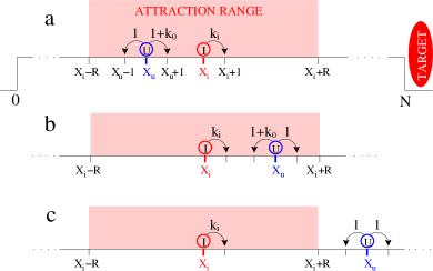
Figure 1: (Color online). Illustration of the model’s dynamics. Informed particle $I$ jumps rightwards with rate $k_{i}$ until it hits the food target at site $N$. (a) and (b) When the uninformed particle $U$ is inside $I$’s attraction range $R$ (red shaded region), it jumps with rate $k_{u}=1+k_{0}$ towards $I$ and with rate $k_{u}=1$ away from $I$. (c) When it is outside that range, $U$ jumps right and left with rate $k_{u}^{\pm}=1$. $U$ stops when it reaches either the absorbing site $0$ or $N$.

$$k_{u}^{+}=\left\{\begin{array}[]{lll}1&\mbox{for}&0<x_{u}<x_{i}-R,\\ 1+k_{0}&\mbox{for}&x_{i}-R\leq x_{u}<x_{i},\\ 1&\mbox{for}&x_{i}\leq x_{u}<N.\end{array}\right.$$

$$k_{u}^{-}=\left\{\begin{array}[]{lll}1&\mbox{for}&0<x_{u}\leq x_{i},\\ 1+k_{0}&\mbox{for}&x_{i}<x_{u}\leq x_{i}+R,\\ 1&\mbox{for}&x_{i}+R<x_{u}<N.\end{array}\right.$$

In other words, particle $I$ moves ballistically towards a known target located at site $N$, while particle $U$ experiments a bias $k_{0}$ towards $I$ when it is within $I$’s interaction range $R$, and moves as a symmetric random walker as long as it is outside this range. Finally, when both particles occupy the same site, $U$ jumps with equal rates $k_{u}^{+}=k_{u}^{-}=1$. Particle $U$ stops walking when it reaches either site $0$ or $N$ (absorbing sites of the system), and particle $I$ stops at site $N+R$, so that the communication between $U$ and $I$ is switched off once $I$ finds the target at $n=N$. Note that if the motion of $U$ were independent of $I$ and performing a symmetric random walk, $U$ would have the same likelihood to reach either end of the chain. However, given that $I$ moves to the right and “attracts” $U$ when they are close enough, one can view the dynamics as $U$ receiving “effective kicks” to the right and, therefore, one expects $U$ to have a preference for the target located at $n=N$.

As indicated in the introduction, this model aims to tackle some of the fundamental questions about the relationship between animal interactions and searching processes. What is the effect of leadership interactions on foraging success? How does the probability of reaching the food target depend on the speed and diffusion of both leading and recruited particles? What happens in a more complex and realistic scenario with many competing leaders? To address these questions we study in the next three sections the cases of one uninformed particle and one or several informed particles. We focus on the probability that $U$ reaches the right target $N$, or first-passage probability $F^{\mbox{\tiny N}}$ to target $N$. Our aim is to explore how this quantity depends on the speed $k_{i}$ of $I$, its attraction range $R$ and the bias $k_{0}$. Within a biological context, $k_{i}$ can be seen as a strategic parameter that an informed animal wants to tune in order to optimize its recruitment strength and maintain group cohesion.

III One informed and one uninformed particles

We start performing numerical simulations of the dynamics described in Section II. As we see in Fig. 2, the first-passage probability (FPP) $F^{\mbox{\tiny N}}$ is non-monotonic in the jumping rate or speed $k_{i}$ of particle $I$, showing its maximum at intermediate speeds. That is, there is an optimal speed denoted by $k_{i}^{*}$, for which the success probability $F^{\mbox{\tiny N}}$ of $U$ is maximum.

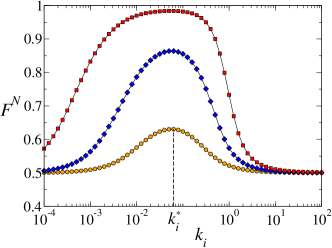
Figure 2: (Color online). Probability $F^{\mbox{\tiny N}}$ that the uninformed particle $U$ reaches target $N$ vs the jumping rate $k_{i}$ of the informed particle, for internal strengths $k_{0}=0.2$ $(\bullet)$, $k_{0}=0.5$ $(\blacklozenge)$ and $k_{0}=1.0$ $(\blacksquare)$. $F^{\mbox{\tiny N}}$ is maximum at $k_{i}^{*}$. Simulations correspond to a chain of length $N=100$ and an attraction range of the informed particle $R=10$.

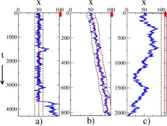
Figure 3: (Color online) Individual realizations of the searching process representing typical trajectories of the particles in three different regimes of the model: (a) small $k_{i}$, (b) optimal search $k_{i}=k_{i}^{*}=0.06$ and (c) large $k_{i}$. Space and time are displayed on the $x$ and $y$ axis, respectively, and the target at site $N=100$ is denoted by a red ellipse. Parameters: $N=100$, $R=10$ and $k_{0}=0.2$. In all plots black dashed lines represent the interaction range, which is centered at the red solid line representing the trajectory of the informed particle, whereas the remaining blue solid line shows the trajectory of the uninformed particle.

We can distinguish three different regimes depending on $I$’s speed: (i) the low speed regime, (ii) the optimal regime $k_{i}\simeq k^{*}_{i}$, and (iii) the high speed regime. Typical trajectories of each case are shown in Figs. 3(a), (b) and (c), respectively. In regime (i) $I$ remains almost static [see Fig. 3 (a)], so jumping rates of $U$ are symmetric around the center of the chain, and $U$ reaches target $N$ with probability $F^{\mbox{\tiny N}}\simeq 1/2$. In this case, $I$ interacts many times with $U$, but its overall effect is null because of the symmetry of its position and interaction. In the other extreme, regime (iii), the interaction between $U$ and $I$ is negligible, given that $I$ moves very fast and quickly leaves $U$ out of its interaction range [see Fig. 3(c)]. Therefore, $U$ performs a symmetric random walk leading to $F^{\mbox{\tiny N}}\simeq 1/2$. Finally, in the intermediate regime (ii), $I$ moves at a speed that “traps” $U$ inside the interaction range most of its way to the target [see Fig. 3(b)]. This “right speed” is not too fast to overtake and leave $U$ behind, but also not too slow to have no effective drag on $U$.

Figure 4 shows that $F^{\mbox{\tiny N}}$ increases from $1/2$ linearly with $k_{i}$ in the very low speed limit, while it decays to $1/2$ as $k_{i}^{-1}$ in the very large $k_{i}$ limit. In the next three subsections we explore each regime in more detail and provide analytic estimations.

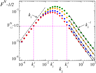
Figure 4: (Color online) First-passage probability of the uninformed particle to target $N$, $F^{\mbox{\tiny N}}$, vs the speed of the informed particle $k_{i}$ on a log-log plot, for chains of length $N=50$ $(\bullet)$, $N=100$ $(\blacksquare)$, $N=200$ $(\blacklozenge)$ and $N=300$ $(\blacktriangledown)$, with $k_{0}=0.2$ and $R=10$. $F^{\mbox{\tiny N}}$ is shifted by $1/2$ to show the asymptotic behaviors $F^{\mbox{\tiny N}}-1/2\sim k_{i}$ and $F^{\mbox{\tiny N}}-1/2\sim k_{i}^{-1}$ in the small and large $k_{i}$ limits, respectively. Solid lines represent the high speed approximation from Eq. (13), while the dashed line corresponds to the low speed approximation (29). Vertical dashed lines denote the positions of the maximum $k_{i}^{*}$ and of two arbitrary speeds $k_{i}^{1}$ and $k_{i}^{2}$ with the same probability $F_{1,2}^{\mbox{\tiny N}}$.

III.1 The large $k_{i}$ regime

In the very high speed limit $k_{i}\to\infty$, the informed particle $I$ reaches target $N$ in a very short time. Thus, the uninformed particle $U$ does not have the chance to make even a single step, staying at the center site of the chain, which we will call site $c\equiv N/2$ from now on. More precisely, given that $I$ jumps in a mean time $1/k_{i}$, when $k_{i}\gg(2+k_{0})(N/2+R)$, $I$ arrives to the target in a mean time $(N/2+R)/k_{i}$, which is much smaller than the typical time $(2+k_{0})^{-1}$ that $U$ needs to make a single jump. This extreme behavior is shown in Fig. 3(c). Hence, after $I$ reaches the target, $U$ performs a symmetric random walk starting from $n=c$, and hitting site $N$ with probability $F^{\mbox{\tiny N}}=1/2$. Now, following the same reasoning, we consider the $k_{i}\gg 2+k_{0}$ limit, that is, $k_{i}$ lower than the extreme value considered before but still high. This corresponds to the case in which the bias in $I$ is much larger than the diffusion of $U$. Given that $I$ moves right much faster than $U$, $U$ makes a few steps before leaving the box through the left side. Therefore, we can assume that once $U$ leaves the box it never comes back in again, because it is very unlikely that $U$ diffusing with a very low rate can catch the very fast moving box. After $U$ leaves the box at a given position $x$, it starts a pure diffusion motion, reaching target $N$ with a probability that increases linearly as we approach to site $n=N$ Redner (2001); Gardiner (2009)

$$F^{\mbox{\tiny N}}=\frac{x}{N}.$$ (3)

In the mean time $\Delta t$ that $U$ takes to leave the box, the box travels a mean distance $k_{i}\,\Delta t$ and, therefore, $U$ leaves the box at position

$$x=\frac{N}{2}+k_{i}\,\Delta t-R-1,$$ (4)

where $R+1$ accounts for the distance between $U$ and the center of the box at the exit moment. The exit time $\Delta t$ can be calculated working in the reference frame of the box, where the relative position of $U$ respect to the box’s center is $x^{\prime}_{u}=x_{u}-x_{i}$, thus $-R\leq x^{\prime}_{u}\leq R$ inside the box. Then $U$ jumps in the box’s reference frame with rates

$$k_{u}^{\prime+}(n) = \left\{\begin{array}[]{ll}1+k_{0}&\mbox{for $-R\leq n\leq-1$,}\\ 1&\mbox{for $0\leq n\leq R$.}\end{array}\right.$$ (7)

$$k_{u}^{\prime-}(n) = \left\{\begin{array}[]{ll}1+k_{i}&\mbox{for $-R\leq n\leq 0$,}\\ 1+k_{0}+k_{i}&\mbox{for $1\leq n\leq R$.}\end{array}\right.$$ (10)

In the limit $k_{i}\gg 2+k_{0}$ considered here, $U$ moves ballistically to the left under a strong bias $k_{i}-k_{0}$, when it is seen from the perspective of the box. Thus the mean exit time corresponds to that of a ballistic motion with $R+1$ left steps: $1$ step and then $R$ steps with effective left rates $k_{i}$ and $k_{i}-k_{0}$, respectively,

$$\Delta t\simeq\frac{1}{k_{i}}+\frac{R}{k_{i}-k_{0}}.$$ (11)

Plugging expression (11) for $\Delta t$ into Eq. (4) gives

$$x\simeq\frac{N}{2}+\frac{k_{0}R}{k_{i}-k_{0}},$$ (12)

and using this expression for $x$ in Eq. (3), we finally obtain

$$F^{\mbox{\tiny N}}=\frac{1}{2}+\frac{k_{0}R}{N(k_{i}-k_{0})}.$$ (13)

As we show in Fig. 4, Eq. (13) reproduces very well the behavior of $F^{\mbox{\tiny N}}$ from numerical simulations in the $k_{i}\gg 2+k_{0}=2.2$ regime. Discrepancies between theory and simulations start to be important for $k_{i}\lesssim 1$. In summary, we showed that the FPP approaches to $1/2$ as $k_{i}^{-1}$ in the large $k_{i}$ limit.

III.2 The small $k_{i}$ regime

In the simplest case $k_{i}=0$, $I$ remains fixed at the center site $c=N/2$. The interval $[c-R,c+R]$, where $U$ feels the presence of $I$, defines an “attracting box” of length $2R$ centered at $I$’s position $x_{i}=c$. One can see the dynamics as $U$ performing a random walk on a chain with quenched right $k_{u}^{+}(n)$ and left $k_{u}^{-}(n)$ site-dependent jumping rates (see Fig. 1)

$$k_{u}^{+}(n)=\left\{\begin{array}[]{ll}1+k_{0}&\mbox{for $c-R\leq n\leq c-1$,}\\ 1&\mbox{otherwise.}\end{array}\right.$$ (16)

$$k_{u}^{-}(n)=\left\{\begin{array}[]{ll}1+k_{0}&\mbox{for $c+1\leq n\leq c+R$,}\\ 1&\mbox{otherwise.}\end{array}\right.$$ (19)

Because of the symmetry of rates around $c$ and of the initial condition $x_{u}(0)=x_{i}(0)=c$, $U$ has the same chance to hit both targets, thus $F^{\mbox{\tiny N}}=1/2$. Now, if $k_{i}$ is larger than zero, $U$ rates $k_{u}^{\pm}(n)$ change every time the box makes a step to the right. Therefore, in this situation rates vary not only along the chain but also on time. This case is hard to analyze, so we focus here on the simplest non-trivial limit of very low $k_{i}$.

We consider the situation in which the typical time $1/k_{i}$ that $I$ takes to make a single step is much smaller than the mean time $T_{c}$ that $U$ needs to reach an end of the chain, starting from site $c$. An exact expression for $T_{c}$ is obtained in Appendix B [see also Eq. (22)]. During the time $T_{c}$, $I$ makes $n$ steps with probability $p_{n}=\frac{k_{i}^{n}T_{c}^{n}}{n!}e^{-k_{i}T_{c}}$. Then, in the $k_{i}\ll 1/T_{c}$ limit these probabilities are reduced to $p_{0}=1-k_{i}T_{c}+\mathcal{O}(k_{i}^{2}T_{c}^{2})$, $p_{1}=k_{i}T_{c}+\mathcal{O}(k_{i}^{2}T_{c}^{2})$, $p_{n}=k_{i}^{n}T_{c}^{n}+\mathcal{O}(k_{i}^{n+1}T_{c}^{n+1})$ for $n\geq 2$. Therefore, neglecting terms of order $k_{i}^{2}T_{c}^{2}\ll 1$ and higher, only two events are statistically possible: (1) the box moves one step to site $n=c+1$, with probability $P_{c+1}=p_{1}=k_{i}T_{c}$, or (2) the box does not move, staying at the initial center site $n=c$, with probability $P_{c}=p_{0}=1-k_{i}T_{c}$. That is, we sort all possible realizations of the dynamics into two classes, those in which $I$ jumps once before $U$ exits the chain and those in which $U$ exits before $I$ makes any jump. If we denote by $F_{c+1}^{\mbox{\tiny N}}$ ($F_{c}^{\mbox{\tiny N}}$) the FPP to target $N$ in the first (second) event, then the FFP can be calculated as

$$F^{\mbox{\tiny N}}=P_{c}\,F_{c}^{\mbox{\tiny N}}+P_{c+1}\,F_{c+1}^{\mbox{\tiny N}}.$$ (20)

In the second event (box does not move), the FPP to target $N$ is simply $F_{c}^{\mbox{\tiny N}}=1/2$, as mentioned before. Then, Eq. (20) is reduced to

$$F^{\mbox{\tiny N}}=\frac{1}{2}+\left(F_{c+1}^{\mbox{\tiny N}}-\frac{1}{2}\right)k_{i}\,T_{c}.$$ (21)

To calculate $T_{c}$ we take advantage of the symmetry of $U$’s jumping rates around $c$, and map the chain $[0,N]$ with absorbing boundaries at sites $0$ and $N$ to a chain $[c,N]$ with reflecting and absorbing boundaries at sites $c$ and $N$, respectively (see Appendix B). We obtain

$$T_{c}=\tau_{e}+\frac{(\tilde{N}-2)\left[(2+k_{0})(1+k_{0})^{R}-2\right]}{4k_{0}}+\frac{\tilde{N}(\tilde{N}-2)}{8},$$ (22)

where we have defined $\tilde{N}\equiv N-2R$, and

$$\tau_{e}=\frac{(2+k_{0})\left[(1+k_{0})^{R+1}-1\right]-2k_{0}(R+1)}{2k_{0}^{2}}$$ (23)

is the mean time that $U$ takes to escape from the box, starting from the center and with the box fixed (see Appendix A). The estimation of $F_{c+1}^{\mbox{\tiny N}}$ involves many steps, which we develop in Appendix C for the interested reader. The approximate final result is

$$F_{c+1}^{\mbox{\tiny N}}\simeq\frac{1}{2}+\frac{8\,\tau_{e}}{\tilde{N}(8\tau_{e}+\tilde{N})}.$$ (24)

Plugging this expression for $F_{c+1}^{\mbox{\tiny N}}$ into Eq. (21) we obtain

$$F^{\mbox{\tiny N}}\simeq\frac{1}{2}+\frac{8\,\tau_{e}\,k_{i}\,T_{c}}{\tilde{N}(8\tau_{e}+\tilde{N})}.$$ (25)

For the parameter values used in simulations $N=50,100,200$ and $300$, $R=10,14,18$ and $22$, $k_{0}=0.2,0.5$ and $0.8$, we can simplify Eqs. (22) and (23) for $T_{c}$ and $\tau_{e}$, by retaining only the leading terms. For instance, the factor $(1+k_{0})^{R+1}$ becomes dominant in Eq. (23), thus we get

$$\tau_{e}\simeq\frac{(2+k_{0})(1+k_{0})^{R+1}}{2k_{0}^{2}}.$$ (26)

Using the simplified Eq. (26), we can rewrite Eq. (22) for $T_{c}$ as

$$T_{c}\simeq\tau_{e}+\frac{k_{0}(\tilde{N}-2)\tau_{e}}{2(1+k_{0})}+\frac{\tilde{N}(\tilde{N}-2)}{8}.$$ (27)

One can also check that $\tau_{e}\gg\tilde{N}$ for most combinations of $N$, $R$ and $k_{0}$. Then, plugging Eq. (27) for $T_{c}$ into Eq. (25) and expanding to first order in $\tilde{N}/\tau_{e}$ we get

$$F^{\mbox{\tiny N}}\simeq\frac{1}{2}+\frac{k_{0}\tau_{e}k_{i}}{2(1+k_{0})}\left[1+\frac{(2+k_{0})\tilde{N}}{8k_{0}\tau_{e}}\right],$$ (28)

where we have used $\tilde{N}\gg 2(1+k_{0})/k_{0}$. Finally, replacing $\tau_{e}$ from Eq. (26) into Eq. (28), and keeping only the leading term we arrive to

$$F^{\mbox{\tiny N}}\simeq\frac{1}{2}+\frac{(2+k_{0})(1+k_{0})^{R}\,k_{i}}{4k_{0}}.$$ (29)

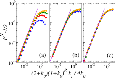
Figure 5: (Color online) Scaling of the first-passage probability of the uninformed particle $F^{\mbox{\tiny N}}$ in the limit of low speed $k_{i}$ of the informed particle, for a chain of length $N=100$ and four values of the attraction range: $R=10\,(\blacktriangledown)$, $R=14\,(\blacklozenge)$, $R=18\,(\blacksquare)$ and $R=22\,(\bullet)$. Each panel corresponds to a different $k_{0}$: (a) $k_{0}=0.2$, (b) $k_{0}=0.5$ and (c) $k_{0}=0.8$. $y$ and $x$ axis were rescaled in order to compare simulation results with the analytic expression (29) (straight solid lines), which corresponds to the straight line $y=x$ in these rescaled axis. Agreement between simulation and theory improves as $k_{0}$ and $R$ increase.

In Fig. 5 we show the asymptotic behavior of the FPP in the small $k_{i}$ limit. $F^{\mbox{\tiny N}}$ is shifted by $1/2$ and the speed $k_{i}$ is rescaled according to the analytic estimation from Eq. (29), denoted by the straight solid line. Simulations correspond to a chain of length $N=100$, while each of the four curves is for a different value of the attraction range $R$. Panels (a), (b) and (c) correspond to strengths $k_{0}=0.2,0.5$ and $0.8$, respectively. We observe that as $R$ and $k_{0}$ increase, the agreement between numerical results and the analytic curve from Eq. (29) improves. This is because as $R$ and $k_{0}$ get larger, the term $(1+k_{0})^{R+1}$ becomes more dominant, and thus the approximate expression for $\tau_{e}$ from Eq. (26) and the assumption $\tau_{e}\gg\tilde{N}$ improve. In Fig. 4, where we plot the FPP vs $k_{i}$ for various system sizes $N$, we can see that $F^{\mbox{\tiny N}}$ does not depend on $N$ for low $k_{i}$, as predicted by Eq. (29). In summary, the FPP to target $N$ in the small $k_{i}$ limit is proportional to $k_{i}$, exponential of $R$ and independent of the chain’s length $N$.

III.3 Optimal regime $k_{i}\simeq k_{i}^{*}$

We have studied in the last two subsections the limiting cases where the informed particle $I$ moves either too slow [Fig. 3(a)] or too fast [Fig. 3(c)], to guide the movement of the uninformed searcher $U$. In this subsection we investigate the properties of the optimal searching regime [Fig. 3 (b)], where the probability that $U$ reaches the right target is maximum, which happens at intermediate values of $I$’s speed $k_{i}$.

A rough estimation of the optimal speed $k_{i}^{*}$ can be obtained if we assume that the asymptotic behaviors of the FPPs in the small and large $k_{i}$ limits from Eqs. (29) and (13), respectively, intersect near the maximum. Equating these two expressions and solving for $k_{i}$ leads to

$$k_{i}^{*}=2k_{0}\sqrt{\frac{R}{N(2+k_{0})(1+k_{0})^{R}}},$$ (30)

which gives the scaling $k_{i}^{*}\sim N^{-1/2}$ obtained from numerical simulations [Fig. 6(a)].

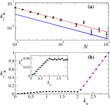
Figure 6: (Color online) (a) Speed of the informed particle $k_{i}^{*}$ that maximizes $F^{\mbox{\tiny N}}$ vs system size $N$ on a double logarithmic scale, obtained from numerical simulations, with $R=10$ and $k_{0}=0.2$. The solid line corresponds to Eq. (30), while the dashed line shows the scaling $k_{i}^{*}\sim N^{-1/2}$. (b) $k_{i}^{*}$ as a function of the free jumping rate $k_{u}$ of the uninformed particle on a chain of length $N=100$. The dashed line is $k_{i}^{*}=k_{u}-2$. Inset: in the low $k_{u}$ regime, data is well fitted by $k_{i}^{*}=0.062\,k_{u}$ (dashed line). $k_{i}^{*}$ is constant in the $1\leq k_{u}\leq 2.062$ interval.

It is also interesting to study the dependence of the optimal speed of $I$ for different values of $U$’s diffusion rates $k_{u}^{\pm}$. Numerical results are shown in Figure 6(b), where we observe three different regimes in the behavior of $k_{i}^{*}$ as a function of $k_{u}^{+}=k_{u}^{-}=k_{u}$:

$$k_{i}^{*}\simeq\left\{\begin{array}[]{lll}0.062\,k_{u}&\mbox{for}&0\leq k_{u}\leq 1,\\ 0.062&\mbox{for}&1\leq k_{u}\leq 2.062,\\ k_{u}-2&\mbox{for}&2.062\leq k_{u}\leq 3.\end{array}\right.$$

That is, $k_{i}^{*}$ is roughly constant for $1\leq k_{u}\leq 2.062$ and grows linearly with $k_{u}$ outside this range. This result is quite intriguing to us, as it is very simple but yet we cannot explain it intuitively. Also, it seems to be quite hard to obtain an analytic estimation of $k_{i}^{*}$ vs $k_{u}$.

IV Two competing informed particles

In Section III we studied the simplest case of two individuals searching for a target, where the leader drags its uninformed partner towards a known target when they are close enough. In this section we consider a more complex situation, consisting of two informed individuals who try to recruit a third uninformed partner. Each leader moves towards different targets located at the opposite ends of the chain. We call them right target $r$ (site $N)$ and left target $l$ (site $0$). The informed particles, denoted by $I_{r}$ and $I_{l}$, start at the center site $c=N/2$ and move ballistically to the right and left with rates $k_{r}$ and $k_{l}$, respectively. The uninformed particle $U$ also starts at site $c$ and diffuses with rates that depend on its relative position respect to $I_{r}$ and $I_{l}$, as in Section III: $U$ has a bias $k_{0}$ towards a given informed particle when it is within its interaction range, and diffuses symmetrically with rates $k_{u}^{+}=k_{u}^{-}=1$ outside that range, as shown in Fig. 7. We can interpret this dynamics as two animals going to opposite located food resources, and trying to convince an undecided conspecific to follow them to their respective resources.

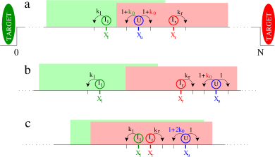
Figure 7: (Color online). Dynamics of two competing informed particles $I_{r}$ and $I_{l}$ traveling in opposite directions at speeds $k_{r}$ and $k_{l}$, respectively. The uninformed particle $U$ experiments a bias $k_{0}$ towards $I_{r}$ and/or $I_{l}$ when it is inside their respective attraction ranges, depicted by the red and green regions, respectively. $U$ symmetrically diffuses with rates $k_{u}^{\pm}=1$ outside that ranges, until it hits either right or left target.

In order to make the analysis of this system as simple as possible we consider two identical leaders that have the same interaction range $R=10$ and attracting strength $k_{0}=0.2$, on a chain of length $N=100$, and vary $k_{r}$ and $k_{l}$. The question we want to explore is: under which conditions one target (leader) is favored respect to the other one? Or, how does the probability of reaching a given target depend on the speeds $k_{r}$ and $k_{l}$?

Figure 8(a) shows in colored scale the probability $F^{\mbox{\tiny N}}$ that particle $U$ reaches the right target $N$, as a function of the speeds of the informed particles, $k_{r}$ and $k_{l}$. Notice that the probability of getting the left target is simply $1-F^{\mbox{\tiny N}}$. The complementary plot in Fig. 8(b) indicates the regions where a given target is favored. White regions correspond to values of $k_{r}$ and $k_{l}$ where $F^{\mbox{\tiny N}}>1/2$ (right target favored), while black regions correspond to $F^{\mbox{\tiny N}}<1/2$ (left target favored). As expected, along the $k_{r}=k_{l}$ line which separates both regions is $F^{\mbox{\tiny N}}=1/2$ (solid line), corresponding to the case of equally fast moving particles. Perfectly identical particles with the same initial conditions must have the same chances to win. Interestingly, as we observe in Fig. 8, the symmetric case $F^{\mbox{\tiny N}}=1/2$ also happens for other combinations of $k_{r}$ and $k_{l}$, indicated by the dashed line. An approximate expression for this crossover line can be obtained by arguing that both informed particles would have the same likelihood to guide $U$ as long as each particle has the same probability to guide $U$ to its target independently, i.e., in the absence of the other informed particle. In other words, one can see the system of three particles as two independent systems; one composed by $U$ and $I_{r}$, and the other by $U$ and $I_{l}$. Then, if $I_{r}$ drags $U$ in the first system with the same probability as $I_{l}$ drags $U$ in the second system, then $I_{r}$ and $I_{l}$ will drag $U$ with the same probability $1/2$ in the combined 3-particle system. This makes sense if we consider the case of one $I$ and one $U$ particles studied in section III. The relation between the FPP $F^{\mbox{\tiny N}}$ of particle $U$ and the speed $k_{i}$ of particle $I$ is plotted in Fig. 4. Because of the non-monotonic shape of $F^{\mbox{\tiny N}}$, $U$ has the same hitting probability for two different speeds $k_{i}^{1}$ and $k_{i}^{2}$ of $I$, that is, $F^{\mbox{\tiny N}}(k_{i}^{1})=F^{\mbox{\tiny N}}(k_{i}^{2})$ [see Fig. 4]. Therefore, we can arbitrarily identify these two speeds with the speeds $\tilde{k}_{r}$ and $\tilde{k}_{l}$ of the right and left informed particles, and find the relation which matches the FPPs to their targets. Then, matching Eq. (29) for $F^{\mbox{\tiny N}}(\tilde{k}_{r})$ with Eq. (13) for $F^{\mbox{\tiny N}}(\tilde{k}_{l})$, in the low and high speed limit, respectively, we obtain

$$\frac{(2+k_{0})(1+k_{0})^{R}\,\tilde{k}_{r}}{4k_{0}}=\frac{k_{0}R}{N\tilde{k}_{l}}.$$ (32)

Finally, pulling $\tilde{k}_{r}$ and $\tilde{k}_{l}$ to the left hand side of Eq. (32), and using expression (30) for the optimal value $k_{i}^{*}$, we arrive to

$$\tilde{k}_{r}\,\tilde{k}_{l}=(k_{i}^{*})^{2}.$$ (33)

Equation (33) gives an estimation of the nontrivial solution corresponding to the dashed straight line in double logarithmic scale $\log\tilde{k}_{l}=2\log k_{i}^{*}-\log\tilde{k}_{r}$ of Fig. 8, with $k_{i}^{*}=0.062$ ($N=100,k_{0}=0.2,R=10$ and $k_{u}=1$).

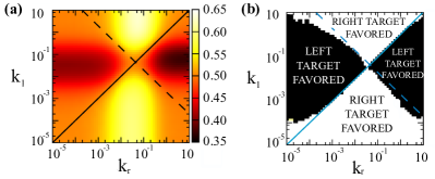
Figure 8: (Color online) (a) Color-scale plot showing the probability $F^{\mbox{\tiny N}}$ that the uninformed particle arrives at the right target $N$ in presence of a right and a left moving particles, as a function of their speeds $k_{r}$ and $k_{l}$. (b) Phase diagram showing the regions in the $k_{l}-k_{r}$ space where the uninformed particle most likely reaches the right (white: $F^{\mbox{\tiny N}}>1/2$) or left (black: $F^{\mbox{\tiny N}}<1/2$) target.

In order to gain a deeper insight about the results reported in Fig. 8, we fix the speed of the left informed particle $k_{l}$ to a given value, and study how the FPPs behave as we vary the speed of the right informed particle $k_{r}$. This is equivalent to analyzing a horizontal cross section of the FPP landscape of Fig. 8. Results for four different speeds $k_{l}$ are shown in Fig. 9(a), where we plot the probability of reaching the right target $F^{\mbox{\tiny N}}$ as a function of the ratio $k_{r}/k_{l}$. We observe the following behavior as $k_{r}$ decreases from high values. For $k_{r}/k_{l}\gg 1$, the very fast moving particle $I_{r}$ has a very short (almost negligible) interaction with $U$, and so we can neglect the presence of $I_{r}$ and only consider the two-particle system composed by $U$ interacting with $I_{l}$, like the one studied in Section III. Therefore, the FPP to the left target $F^{\mbox{\tiny 0}}(k_{l})$ has the functional form of the FPP plotted in Fig. 4, where $k_{l}$ takes only the four values $k_{l}=10^{0},10^{-1},10^{-2}$ and $10^{-3}$ of Fig. 9(a). We make clear here that the $F^{\mbox{\tiny N}}$ vs $k_{i}$ curve of Fig. 4 corresponds to the FPP to the right target when the informed particle $I$ moves right, but it must be equivalent to the FPP to the left target when $I$ moves left. Then, particle $U$ reaches the right target with the complementary probability $F^{\mbox{\tiny N}}=1-F^{\mbox{\tiny 0}}(k_{l})$, which agrees with the asymptotic value of $F^{\mbox{\tiny N}}<1/2$ in the $k_{r}/k_{l}\gg 1$ limit [Fig. 9(a)]. As $k_{r}$ decreases, $F^{\mbox{\tiny N}}$ increases, given that $I_{r}$ starts influencing the motion of $U$, until it reaches a maximum. Then, as $I_{r}$ moves even more slowly $F^{\mbox{\tiny N}}$ decreases, reaching an asymptotic value in the $k_{r}/k_{l}\ll 1$ limit corresponding to an almost static $I_{r}$. We also observe that $F^{\mbox{\tiny N}}$ takes the value $1/2$ in two points, indicated by vertical dashed lines, one corresponding to $k_{r}=k_{l}$ and the other to the nontrivial value approximated by Eq. (33) (dashed line of Fig. 8). The theoretical value $\tilde{k}_{r}=(k_{i}^{*})^{2}/\tilde{k}_{l}$ agrees well with numerical simulations only close to the $k_{l}=k_{r}=k_{i}^{*}$ point, as we can see in Fig. 8, where the solid and dashed lines cross. However, discrepancies increase as we move away from $k_{l}=k_{r}=k_{i}^{*}$ because the theoretical value of $k_{i}^{*}$ from Eq. (30) underestimates the numerical value, as Fig. 6(a) shows.

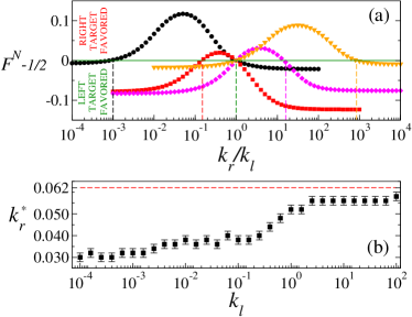
Figure 9: (a) (Color online) Probability $F^{\mbox{\tiny N}}$ that the uninformed particle reaches the right target $N$ as a function of the ratio $k_{r}/k_{l}$ between the speeds of the right and left moving particles. Each curve correspond to a fixed speed $k_{l}$ [$k_{l}=1.0(\bullet),k_{l}=10^{-1}(\blacksquare),k_{l}=10^{-2}(\blacklozenge)$ and $k_{l}=10^{-3}(\blacktriangledown)$]. Vertical dashed lines denote the crossing points where $F^{\mbox{\tiny N}}=1/2$. (b) Optimal speed of the right-moving particle $k_{r}^{*}$ that maximizes $F^{\mbox{\tiny N}}$ as a function of the speed $k_{l}$ of its competing partner. The horizontal dashed line indicates the asymptotic value $k_{r}^{*}=0.062$ in the $k_{l}\to\infty$ limit.

As we can see, the right-moving particle has to adapt its speed to the speed of the left-moving competitor in order to have the greatest chances to take the uninformed searcher to the right target. A direct consequence of this observation is the fact that the optimal speed $k_{r}^{*}$ which maximizes $F^{\mbox{\tiny N}}$ depends on $k_{l}$. This is shown in Fig. 9(b), where we see that $k_{r}^{*}$ increases with $k_{l}$. In the high speed limit $k_{l}\to\infty$ of the left particle, $I_{l}$ has no effect on $U$, thus $k_{r}^{*}$ asymptotically reaches the optimal value $k_{i}^{*}=0.062$ of the two-particle system [see Fig. 9(b)]. As $k_{l}$ decreases from very high values, $I_{l}$ starts dragging $U$ to the left, so $I_{r}$ has to move slower to compensate this effect and maximize $F^{\mbox{\tiny N}}$, monotonically reducing the value of $k_{r}^{*}$.

V Competing groups of informed particles

In the last section we studied the case in which two different leaders move in opposite directions. But in a more general scenario one can have two competing groups of leaders. Our aim in this section is to explore what happens when the two groups have a different size and persuading strength. To that end we study a simple case consisting of two particles moving to the left, one particle moving to the right, and one uninformed diffusing particle $U$ looking for a target. Naturally, the existence of two leaders moving left increases the chances that the uninformed particle reaches the left target. However, as we shall see, for some relations between the attraction strengths and speeds of both groups, the minority may have the largest chances to win.

We start studying the case in which all three informed particles have the same interaction strength $k_{0}=0.2$ and range $R=10$. The two-particle group (majority) moves left with speed $k_{\mbox{\tiny M}}$, while the one-particle group (minority) moves to the right with speed $k_{m}$. Initially, all four particles are at the center of the chain. The presence of a majority preferring the left target breaks the symmetry of the model studied in Section IV. Indeed, Fig. 10 shows that the majority (left) target has the largest probability of being reached by $U$, for most combinations of $k_{\mbox{\tiny M}}$ and $k_{m}$. Only when the majority moves either too fast or too slow the minority manages to take $U$ to the right target. These two limiting situations are slightly different. In the $k_{\mbox{\tiny M}}\to 0$ limit, the left-moving majority remains static at the center and, therefore, have no any bias effect on $U$. But the right-moving minority introduces a bias to the right, as we know from section III, giving an overall right bias that favors the minority (right) target. In the $k_{\mbox{\tiny M}}\to\infty$ limit the majority can be neglected, as it has a extremely short interaction with $U$, thus the minority moving at finite speed has the largest chances to win. Interestingly, in the $10^{-3}\leq k_{\mbox{\tiny M}}\leq 2\times 10^{-1}$ range, the majority target is favored for all speeds $k_{m}$, that is, the majority usually wins when moving at intermediate speeds, independent on the minority’s speed.

Finally, it is interesting to study the case where the two groups have different internal strengths. In order to counterbalance the numerical advantage of the majority group, we double the strength of the particle in the minority, to the value $2k_{0}=0.4$, but keep the strength of both particles in the majority in the value $k_{0}=0.2$. Then, the total majority strength $2k_{0}$ acting on $U$ matches that of the minority. With these parameters, the two targets seem to be equivalent, as it happens for the case of two identical informed particles studied en Section IV. However, as we observe in Fig. 11, the probability of arriving at the minority target is largest for most $k_{\mbox{\tiny M}}-k_{m}$ combinations (white region), showing that there is a preference for the minority target. This is specially evident around the $k_{\mbox{\tiny M}}=k_{m}=k_{i}^{*}=0.062$ region (green dot). Indeed, when both the majority and the minority set their speeds equal and close to the single-particle optimal speed $k_{i}^{*}$, the minority is more efficient in dragging $U$ to its target. Seemingly, the fact that the total strength $2k_{0}$ of the majority is divided among two particles causes a less effective dragging force on $U$ than that caused by a single particle with strength $2k_{0}$. An insight about this result can be obtained with the following reasoning. If both particles in the majority would move together in perfect synchrony, then their interaction ranges would always overlap along the path to the target, and they would behave as a single particle with strength $2k_{0}$. However, stochasticity in the jumping process splits particles apart, introducing two competing effects. On the one hand, the total interaction range composed by the range of the two left-moving particles is larger than that of the right-moving particle, seemingly inducing an effective left drag over $U$. But, on the other hand, the strength of this total interaction range is $2k_{0}$ only where the ranges of both left-moving particles overlap, and $k_{0}$ where they do not overlap, which is only half of the strength of the right-moving particle. Apparently, this last mechanism induced by the difference in strengths is stronger than the effect produced by enlarging the interaction range, consequently breaking the symmetry in favor of the right target.

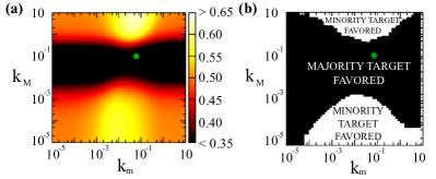
Figure 10: (Color online) (a) Probability (color-scale) that the uninformed particle arrives at the minority (right) target, under the influence of two informed particles moving to the left at speed $k_{\mbox{\tiny M}}$ and one to the right at speed $k_{m}$. All three informed particles have the same internal strength $k_{0}=0.2$ and interaction range $R=10$. (b) Regions in the $k_{\mbox{\tiny M}}-k_{m}$ speed space where the uninformed particle has the largest chances to reach the minority (right) or majority (left) target. The largest region corresponds to the majority target favored. The green dot indicates the optimal speed $k_{\mbox{\tiny M}}=k_{m}=0.062$.

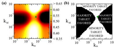
Figure 11: (Color online). Same as in Fig. 10 but for the case in which the strength $2k_{0}=0.4$ of the right-moving particle is twice the strength $k_{0}=0.2$ of each of the two left-moving particles. The probability that the uninformed particle reaches the minority (right) target are largest for most combinations of speeds $k_{\mbox{\tiny M}}$ and $k_{m}$ (white region).

VI Summary and conclusions

In this article we have presented a minimalist approach to study how the presence of a leader in a group of animals may influence the movement of its conspecifics and incidentally their searching efficiency. The model has two types of individuals: informed leaders that move ballistically at speed $k_{i}$ towards the location of a known target, and uninformed searchers that are attracted towards leaders when they are close enough, but they freely diffuse with rate $k_{u}$ otherwise. To quantify the benefits of following the leader, we have focused on the probability $F^{\mbox{\tiny N}}$ that the uninformed searcher finds a specific target $N$, and studied how that depends on $k_{i}$, $k_{u}$ and the internal attraction strength $k_{0}$.

We started analyzing the simplest case where there is only one individual of each type. We found that the first-passage probability $F^{\mbox{\tiny N}}$ is non-monotonic and reaches its maximum at an intermediate value $k_{i}^{*}$ that is proportional to $k_{u}$. Therefore, searching efficiency is maximized when the informed particle moves at intermediate speeds, as compared to the diffusion of the uninformed particle. If it moves too fast there is almost no interaction, and if it moves too slow the interaction has almost no net effect on the final destination of the uninformed particle, which is not able to take advantage of the information exchange. Moving not too fast but also not too slow seems to be the optimal strategy to recruit undecided particles when they have a fixed diffusion rate.

Then, we considered a more general situation in which two identical leaders moving in opposite directions compete for an uninformed individual. It turns out that the particle that adapts its speed to a value closer to the optimal speed $k_{i}^{*}$ has the largest chances to win. Surprisingly, a tie is obtained for a nontrivial relationship between the speed of both particles, besides the case where they move at the same speed. When a group of two leaders compete against a single particle group, the largest group wins for most combinations of speeds, as its combined effective persuading force is stronger. However, this situation is reversed when the social strength of the smaller group is doubled. Therefore, by following two different strategies a minority may be able to beat a majority: either by increasing its internal strength or by adapting its speed to an optimal value relative to the speed of the majority.

It would be worthwhile to explore some extensions of the model that include, for instance, many uninformed particles that interact not only with the leaders but also between them. Also, in a more realistic scenario informed particles would not be identical but each would have a different strength and range of interaction, and they may also have some diffusion, instead of the pure ballistic motion considered in the present work.

VII Acknowledgments

R.M-G. is supported by the JAEPredoc program of CSIC. R.M-G. and C.L acknowledge support from MINECO (Spain) and FEDER (EU) through Grants No. FIS2012-30634 (INTENSE@COSYP) and CTM2012-39025-C02-01 (ESCOLA).

Appendix A Calculation of the mean escape time from the attractive box $\tau_{e}$

In this section we calculate the mean time $\tau_{e}$ that particle $U$ takes to escape from the attracting box, when the box is static. Given that the position of the box is irrelevant in this case we assume, for simplicity, that the box is centered at $n=0$. Then $\tau_{e}$ is equivalent to the mean exit time from an interval $[-R,R]$, starting from $n=0$ or, equivalently, the mean first-passage (MFPT) time to either site $n=-R-1$ or $n=R+1$. Given that jumping rates are symmetric around $n=0$, we can view the left half interval $[-R-1,0]$ as a mirrored image of the right half $[0,R+1]$. In this simpler scenario, we can consider the particle $U$ as confined in a chain $[0,R+1]$ with a reflecting wall at $n=0$ and an absorbing site at $n=R+1$. Therefore, our problem is reduced to the MFPT to site $R+1$, starting from the reflecting boundary $0$, with jumping rates

$$k_{u}^{+}(n) = \left\{\begin{array}[]{ll}2&\mbox{for $n=0$,}\\ 1&\mbox{for $1\leq n\leq R$.}\end{array}\right.$$ (36)

$$k_{u}^{-}(n) = 1+k_{0}~{}~{}~{}~{}\mbox{for $1\leq n\leq R$.}$$ (37)

We note that the jumping rate $k_{0}^{+}=2$ at site $0$ is twice the outgoing rate from $0$ in the complete chain. The MFPT starting from site $n$, $T(n)$, obeys the recursion equation Gardiner (2009)

$$k_{u}^{+}(n)\left[T(n+1)-T_{n}\right]+k_{u}^{-}(n)\left[T(n-1)-T(n)\right]=-1.$$ (38)

The solution of Eq. (38) with reflecting and absorbing boundary conditions $T(-1)=T(0)$ and $T(R+1)=0$ at $n=0$ and $n=R+1$, respectively, is given by Gardiner (2009)

$$T(n) = \sum_{y=n}^{R}\phi(y)\sum_{z=0}^{y}\frac{1}{k_{u}^{+}(z)\,\phi(z)},~{}~{}~{}\mbox{with}$$

$$\phi(y) = \prod_{z=1}^{y}\frac{k_{u}^{-}(z)}{k_{u}^{+}(z)}.$$

Using rates in Eq. (37) gives $\phi(y)=r^{y}$ ($0\leq y\leq R$), where $r\equiv 1+k_{0}$ is the ratio between left and right rates. Replacing the expression for $\phi(y)$ and for the rates $k_{u}^{+}(n)$ from Eq. (37), the MFPT starting from site $n=0$ can be expressed as

$$\tau_{e}\equiv T(0)=\sum_{y=0}^{R}r^{y}\sum_{z=0}^{y}\frac{1}{k_{u}^{+}(z)\,r^{z}}=\sum_{y=0}^{R}r^{y}\left[\frac{1}{2}+\sum_{z=1}^{y}r^{-z}\right].$$

(39)

To perform the sums in Eq. (39) we make use of the equivalence $\sum_{k=0}^{M-1}\alpha^{k}=\frac{1-\alpha^{M}}{1-\alpha}$ for the sum of a finite number of terms on a geometric series. Finally, after doing some algebra we arrive to

$$\tau_{e}=\frac{(r+1)(r^{R+1}-1)-2(r-1)(R+1)}{2(r-1)^{2}},$$

or, in terms of the bias $k_{0}=r-1$,

$$\tau_{e}=\frac{(2+k_{0})\left[(1+k_{0})^{R+1}-1\right]-2k_{0}(R+1)}{2k_{0}^{2}},$$

which is the expression quoted in Eq. (23).

Appendix B Calculation of the mean exit time from the chain $T_{c}$

In this section we calculate the mean time that particle $U$ takes to exit the chain, starting from the center site $c=N/2$, when the box is fixed and centered at $c$. Therefore, $U$ diffuses along the chain with site-dependent jumping rates given by Eq. (19). As we did in Appendix A, we take advantage of the system’s symmetry around $c$ and map the chain $[0,N]$ with absorbing boundaries at the extreme sites $n=0,N$, into the chain $[c,N]$ with reflecting and absorbing boundaries at sites $n=c$ and $n=N$, respectively. This mapping drastically reduces the complexity of calculations. Thus, the mean exit time corresponds to the mean first-passage time (MFPT) to the absorbing boundary $N$, starting from the reflecting boundary $c$, and jumping rates

$$k_{u}^{+}(n) = \left\{\begin{array}[]{ll}2&\mbox{for $n=c$,}\\ 1&\mbox{for $c+1\leq n\leq N-1$.}\end{array}\right.$$ (42)

$$k_{u}^{-}(n) = \left\{\begin{array}[]{ll}1+k_{0}&\mbox{for $c+1\leq n\leq c+R$,}\\ 1&\mbox{for $c+R+1\leq n\leq N-1$.}\end{array}\right.$$ (45)

The rate $k_{u}^{+}(c)=2$ is twice the outgoing rate from $c$ in the original chain. The MFPT $T(n)$ starting from site $n$ obeys the recursion formula

$$k_{u}^{+}(n)\left[T(n+1)-T_{n}\right]+k_{u}^{-}(n)\left[T(n-1)-T(n)\right]=-1,$$

whose solution with reflecting and absorbing boundary conditions $T_{c-1}=T_{c}$ and $T_{\mbox{\tiny N}}=0$, respectively, is given by Gardiner (2009)

$$T(n)=\sum_{y=n}^{N-1}\phi(y)\sum_{z=c}^{y}\frac{1}{k_{u}^{+}(z)\,\phi(z)}~{}~{}~{}~{}\mbox{with}~{}~{}~{}~{}\phi(y)=\prod_{z=c+1}^{y}\frac{k_{u}^{-}(z)}{k_{u}^{+}(z)}.$$

Using rates (45) gives

$$\phi(y)=\left\{\begin{array}[]{ll}r^{y-c}&\mbox{for $c\leq y\leq c+R$,}\\ r^{R}&\mbox{for $c+R+1\leq y\leq N-1$,}\end{array}\right.$$ (48)

where $r\equiv 1+k_{0}$. Using rates $k_{u}^{+}(n)$ from Eqs. (45) and $\phi(y)$ from Eq. (48), the MFPT starting from $c$ is

$$T_{c}=T(c)=\sum_{y=c}^{N-1}\phi(y)\sum_{z=c}^{y}\frac{1}{k_{u}^{+}(z)\,\phi(z)}=\sum_{y=c}^{c+R}r^{y-c}\left[\frac{1}{2}+\sum_{z=c+1}^{y}r^{c-z}\right]+\sum_{y=c+R+1}^{N-1}r^{R}\left[\frac{1}{2}+\sum_{c+1}^{c+R}r^{c-z}+\sum_{z=c+R+1}^{y}r^{-R}\right],$$ (49)

where we have split the sum over $z$ in site $c$ and intervals $[c+1,c+R]$ and $[c+R+1,y]$, and the sum over $y$ in intervals $[c,c+R]$ and $[c+R+1,N-1]$. Performing the sums in brackets we obtain

$$T_{c} = \sum_{y=c}^{c+R}r^{y-c}\left[\frac{1}{2}+\frac{1-r^{c-y}}{r-1}\right]+\sum_{y=c+R+1}^{N-1}r^{R}\left[\frac{1}{2}+\frac{1-r^{-R}}{r-1}+r^{-R}\left(y-c-R\right)\right]$$

$$= \sum_{y=0}^{R}\left[\frac{r^{y}}{2}+\frac{r^{y}-1}{r-1}\right]+\sum_{y=1}^{c-R-1}\left[\frac{r^{R}}{2}+\frac{r^{R}-1}{r-1}+y\right].$$

In the last equality, we have made a change of variables and redistributed the terms. Finally, performing the sums and replacing back $r$ by $1+k_{0}$ we arrive to

$$T_{c}=\frac{(2+k_{0})\left[(1+k_{0})^{R+1}-1\right]-2k_{0}(R+1)}{2k_{0}^{2}}+\frac{(\tilde{N}-2)\left[(2+k_{0})(1+k_{0})^{R}-2\right]}{4k_{0}}+\frac{\tilde{N}(\tilde{N}-2)}{8},$$ (50)

where $\tilde{N}\equiv N-2R$. The first term in Eq. (50) exactly agrees with the calculated mean escape time from the box $\tau_{e}$ given by Eq. (23). Expressing this first term as $\tau_{e}$ leads to the expression quoted in Eq. (22).

Appendix C Estimation of the first-passage probability $F_{c+1}^{\mbox{\tiny N}}$

We now find an approximate expression for the FPP $F_{c+1}^{\mbox{\tiny N}}$ to target $N$ when the box jumps to site $n=c+1$ before particle $U$ exits the chain. An exact calculation of $F_{c+1}^{\mbox{\tiny N}}$ is hard to perform because this implies finding the occupation probability of $U$ along the chain for all times. It proves useful to divide the exit dynamics into two stages. During the first stage $U$ diffuses along the chain with jumping rates corresponding to the box centered at $c$, as shown in Eq. (19). Then, the box jumps one step right and $U$ diffuses during a second stage with jumping rates given by

$$k_{u}^{+}(n) = \left\{\begin{array}[]{ll}1+k_{0}&\mbox{for $c-R+1\leq n\leq c$,}\\ 1&\mbox{otherwise,}\end{array}\right.$$ (53)

$$k_{u}^{-}(n) = \left\{\begin{array}[]{ll}1+k_{0}&\mbox{for $c+1\leq n\leq c+R+1$,}\\ 1&\mbox{otherwise,}\end{array}\right.$$ (56)

until it hits one of the two targets. Therefore, the probability to hit target $N$ in a given realization of the dynamics depends on the position of $U$ at the beginning of this second stage, that is, right after the box moves. Thus, $F_{c+1}^{\mbox{\tiny N}}$ can be estimated as

$$F_{c+1}^{\mbox{\tiny N}}=\sum_{n=0}^{N}P(n)F_{c+1}^{\mbox{\tiny N}}(n),$$ (57)

where $P(n)$ is the probability that $U$ is at site $n$ when the box moves to site $c+1$, and $F_{c+1}^{\mbox{\tiny N}}(n)$ is the FPP to target $N$ starting from site $n$, when the box is centered at $c+1$. In Appendix D we show that

$$F_{c+1}^{\mbox{\tiny N}}(n)\simeq\left\{\begin{array}[]{ll}F_{c}^{\mbox{\tiny N}}(n)+\frac{1}{\tilde{N}}&\mbox{for $c-R+1\leq n\leq c+R$,}\\ F_{c}^{\mbox{\tiny N}}(n)&\mbox{otherwise,}\end{array}\right.$$ (60)

where $F_{c}^{\mbox{\tiny N}}(n)$ is the FPP to target $N$ starting from site $n$, with the box centered at $c$. These FPPs obey the boundary conditions $F_{c}^{\mbox{\tiny N}}(0)=F_{c+1}^{\mbox{\tiny N}}(0)=0$ and $F_{c}^{\mbox{\tiny N}}(N)=F_{c+1}^{\mbox{\tiny N}}(N)=1$. The following two properties prove useful in performing the sum of Eq. (57):

$$P(c-n)=P(c+n)~{}~{}~{}\mbox{and}~{}~{}~{}$$ (61)

$$F_{c}^{\mbox{\tiny N}}(c-n)+F_{c}^{\mbox{\tiny N}}(c+n)=1~{}~{}~{}\mbox{for $0\leq n\leq c$},$$ (62)

which reflect the symmetry of the system and initial conditions around $c$. That is, given that $U$ diffuses during the first stage under a symmetric landscape of rates, the occupation probability $P(n)$ must be symmetric around $c$ [Eq. (61)]. In addition, Eq. (62) reflects the fact that the exiting probabilities through $0$ and $N$, starting from the same distance to those borders must be equal, as we explicitly show in Appendix D. From relations (61) and (62) one finds

$$\sum_{n=0}^{N}P(n)F_{c}^{\mbox{\tiny N}}(n)=1/2.$$ (63)

Then, using expressions (60) for $F_{c+1}^{\mbox{\tiny N}}(n)$ in the sum of Eq. (57), and the relation (63), we obtain

$$F_{c+1}^{\mbox{\tiny N}}=\sum_{n=0}^{N}P(n)F_{c}^{\mbox{\tiny$N$}}(n)+\frac{1}{\tilde{N}}\sum_{n=c-R+1}^{c+R}P(n)\simeq\frac{1}{2}+\frac{P_{\mbox{\tiny}box}}{\tilde{N}},$$ (64)

where we have defined $P_{\mbox{\tiny}box}\equiv\sum_{n=c-R}^{c+R}P(n)$, as the probability that $U$ is inside the box when the box jumps. An approximate expression for $P_{\mbox{\tiny}box}$ can be obtained by noting that the likelihood that $U$ is inside the box, i e., in the interval $[c-R,c+R]$, when it has not reached any target yet, should be proportional to the rate at which $U$ enters the box $8/\tilde{N}$, as compared to the rate at which $U$ leaves the box $1/\tau_{e}$ (see Appendix E). Therefore, we arrive to

$$P_{\mbox{\tiny}box}\simeq\frac{8\tau_{e}}{8\tau_{e}+\tilde{N}}.$$ (65)

Finally, plugging Eq. (65) for $P_{\mbox{\tiny}box}$ into Eq. (64) for $F_{c+1}^{\mbox{\tiny N}}$ we arrive to the expression quoted in Eq. (24) of the main text.

Appendix D Estimation of the first-passage probability $F_{c+1}^{\mbox{\tiny N}}(n)$

We calculate in this section the probability $F_{c+1}^{\mbox{\tiny N}}(n)$ that particle $U$ hits target $N$ starting from site $n$, when the box is centered at site $c+1$. In principle, we expect this probability to be very similar to the hitting probability $F_{c}^{\mbox{\tiny N}}(n)$ starting from site $n$ and with the box centered at $c$, instead of $c+1$. In fact, as we shall see, these two probabilities only differ in a small “perturbation” of order $1/\tilde{N}$. We first illustrate how to calculate $F_{c}^{\mbox{\tiny N}}(n)$, and then apply the same technique to calculate $F_{c+1}^{\mbox{\tiny N}}(n)$.

Given that FFPs are unequivocally determined by the right and left jumping probabilities at different sites $p_{n}^{+}$ and $p_{n}^{-}$, respectively, it turns out more convenient to work in discrete time. That is, we see particle $U$ as making either a right or a left step in a time interval $\Delta t=1/K$, where $K=2+k_{0}$ ($K=2$) is the total jumping rate when $U$ is inside (outside) the box. From Eq. (19), jumping probabilities can be written as

$$p_{n}^{+} = \left\{\begin{array}[]{lll}p&\mbox{for $c-R\leq n\leq c-1$,}\\ q&\mbox{for $c+1\leq n\leq c+R$,}\\ \frac{1}{2}&\mbox{otherwise,}\end{array}\right.$$

$$p_{n}^{-} = \left\{\begin{array}[]{lll}q&\mbox{for $c-R\leq n\leq c-1$,}\\ p&\mbox{for $c+1\leq n\leq c+R$,}\\ \frac{1}{2}&\mbox{otherwise,}\end{array}\right.$$

where $p\equiv(1+k_{0})/(2+k_{0})$ and $q\equiv 1/(2+k_{0})$. Note that $p+q=1$. $F_{c}^{\mbox{\tiny N}}(n)$ obeys the following recursion equations

$$F(n) = \frac{1}{2}F(n-1)+\frac{1}{2}F(n+1)~{}~{}~{}~{}~{}\mbox{for~{}~{}~{}~{} $1\leq n\leq c-R-1$,}$$

$$F(n) = qF(n-1)+pF(n+1)~{}~{}~{}~{}~{}~{}\mbox{for~{}~{}~{}~{} $c-R\leq n\leq c-1$,}$$

$$F(n) = \frac{1}{2}F(c-1)+\frac{1}{2}F(c+1)~{}~{}~{}~{}~{}~{}\mbox{for~{}~{}~{}~{} $n=c$,}$$

$$F(n) = pF(n-1)+qF(n+1)~{}~{}~{}~{}~{}~{}\mbox{for~{}~{}~{}~{} $c+1\leq n\leq c+R$,}$$

$$F(n) = \frac{1}{2}F(n-1)+\frac{1}{2}F(n+1)~{}~{}~{}~{}~{}\mbox{for~{}~{}~{}~{} $c+R+1\leq n\leq N-1$,}$$ (68)

where we have dropped indices $c$ and $N$ to simplify notation. The solution to the system of equations (68), subject to absorbing boundary conditions at site $0$ and $N$, $F(0)=0$ and $F(N)=1$, respectively, is given by

$$F_{c}^{\mbox{\tiny N}}(n)=\left\{\begin{array}[]{lllll}A(r-1)n&\mbox{for~{}~{}~{}~{} $0\leq n\leq c-R$,}\\ \frac{A}{2}\left[(r-1)\tilde{N}+2\left(1-r^{c-R-n}\right)\right]&\mbox{for~{}~{}~{}~{} $c-R\leq n\leq c$,}\\ \frac{1}{2}&\mbox{for~{}~{}~{}~{} $n=c$,}\\ \frac{A}{2}\left[(r-1)\tilde{N}+2\left(1-2r^{-R}\right)+2r^{n-c-R}\right]&\mbox{for~{}~{}~{}~{} $c\leq n\leq c+R$,}\\ A\left[(r-1)(n-2R)+2\left(1-r^{-R}\right)\right]&\mbox{for~{}~{}~{}~{} $c+R\leq n\leq N$,}\end{array}\right.$$ (74)

where $r\equiv p/q=1+k_{0}$ and $A\equiv\left[(r-1)\tilde{N}+2\left(1-r^{-R}\right)\right]^{-1}$. We have also placed back indices $c$ and $N$. We can check that $F_{c}^{\mbox{\tiny N}}(c-n)+F_{c}^{\mbox{\tiny N}}(c+n)=1$, with $0\leq n\leq c$, the symmetry property expressed in Eq. (62) of appendix C.

To calculate $F_{c+1}^{\mbox{\tiny N}}(n)$ we follow the same method as for $F_{c}^{\mbox{\tiny N}}(n)$, but with jumping probabilities corresponding to the box centered at $c+1$

$$p_{n}^{+} = \left\{\begin{array}[]{lll}p&\mbox{for $c-R+1\leq n\leq c$,}\\ q&\mbox{for $c+2\leq n\leq c+R+1$,}\\ \frac{1}{2}&\mbox{otherwise.}\end{array}\right.$$

$$p_{n}^{-} = \left\{\begin{array}[]{lll}q&\mbox{for $c-R+1\leq n\leq c$,}\\ p&\mbox{for $c+2\leq n\leq c+R+1$,}\\ \frac{1}{2}&\mbox{otherwise.}\end{array}\right.$$

We obtain

$$F_{c+1}^{\mbox{\tiny N}}(n)=\left\{\begin{array}[]{lllll}A(r-1)n&\mbox{for~{}~{}~{}~{} $0\leq n\leq c-R+1$,}\\ \frac{A}{2}\left[(r-1)\tilde{N}+2r\left(1-r^{c-R-n}\right)\right]&\mbox{for~{}~{}~{}~{} $c-R+1\leq n\leq c+1$,}\\ \frac{A}{2}\left[(r-1)\tilde{N}+2r\left(1-r^{-R-1}\right)\right]&\mbox{for~{}~{}~{}~{} $n=c+1$,}\\ \frac{A}{2}\left[(r-1)\tilde{N}+2r\left(1-2r^{-R-1}\right)+2r^{n-c-R-1}\right]&\mbox{for~{}~{}~{}~{} $c+1\leq n\leq c+R+1$,}\\ A\left[(r-1)(n-2R)+2\left(1-r^{-R}\right)\right]&\mbox{for~{}~{}~{}~{} $c+R+1\leq n\leq N$.}\end{array}\right.$$

$F_{c+1}^{\mbox{\tiny N}}(n)$ can be written in terms of $F_{c}^{\mbox{\tiny N}}(n)$ from Eq. (74) as

$$F_{c+1}^{\mbox{\tiny N}}(n)=F_{c}^{\mbox{\tiny N}}(n)+\left\{\begin{array}[]{lllll}0&\mbox{for~{}~{}~{}~{} $0\leq n\leq c-R$,}\\ A(r-1)\left(1-r^{c-R-n}\right)&\mbox{for~{}~{}~{}~{} $c-R\leq n\leq c$,}\\ A(r-1)\left(1-r^{-R}\right)&\mbox{for~{}~{}~{}~{} $n=c$,}\\ A(r-1)\left(1-r^{n-c-R-1}\right)&\mbox{for~{}~{}~{}~{} $c+1\leq n\leq c+R+1$,}\\ 0&\mbox{for~{}~{}~{}~{} $c+R+1\leq n\leq N$.}\end{array}\right.$$ (83)

Finally, expanding Eq. (83) to first order in $1/r=1/(1+k_{0})<1$, $F_{c+1}^{\mbox{\tiny N}}(n)$ can be reduced to the simple approximate expression

$$F_{c+1}^{\mbox{\tiny N}}(n)\simeq F_{c}^{\mbox{\tiny N}}(n)+\left\{\begin{array}[]{lll}0&\mbox{for~{}~{}~{}~{} $0\leq n\leq c-R$,}\\ \frac{1}{\tilde{N}}&\mbox{for~{}~{}~{}~{} $c-R+1\leq n\leq c+R$,}\\ 0&\mbox{for~{}~{}~{}~{} $c+R+1\leq n\leq N$,}\end{array}\right.$$

quoted in Eq. (60) of appendix C.

Appendix E Estimation of the occupation probability inside the box $P_{box}$

We calculate here an approximate expression for the probability $P_{box}$ that particle $U$ is inside the box, i.e., located at a site $n$ in the range $c-R\leq n\leq c+R$, when the box jumps one step right. We shall see that $P_{box}$ can be estimated as the ratio between the rates associated to $U$ entering and leaving the box.

Within a very simplified coarse-grained picture of the system, we consider that if particle $U$ did not exit the chain, it can be in only two possible occupation states, either inside the box (state $1$) or outside the box (state $0$). That is, states $1$ and $0$ correspond to $U$ being at sites $|n-c|\leq R$ and $|n-c|>R$, respectively. Occupation probabilities $P_{0}(t)$ and $P_{1}(t)$ of states $0$ and $1$ at time $t$ evolve following these master equations

$$\frac{\partial P_{0}(t)}{\partial t}=k_{10}P_{1}(t)-k_{01}P_{0}(t),$$

$$\frac{\partial P_{1}(t)}{\partial t}=k_{01}P_{0}(t)-k_{10}P_{1}(t),$$ (85)

where $k_{10}$ ($k_{01}$) is the transition rate from inside (outside) to outside (inside) the box. The total occupation probability is normalized to one [$P_{0}(t)+P_{1}(t)=1$], because we restrict to the case where the particle is still inside the chain. If we run many realizations of the dynamics, this means that at a given time $t$ we only consider those realizations in which $U$ did not exit the chain, and associate $P_{1}(t)$ with the fraction of those realizations where $U$ is inside the box. The solution to Eqs. (85) with initial condition $P_{i}(t)=\delta_{i,1}$ ($U$ inside the box) is

$$P_{0}(t)=\frac{k_{10}\left[1-e^{-(k_{01}+k_{10})t}\right]}{k_{01}+k_{10}},$$

$$P_{1}(t)=\frac{k_{01}+k_{10}e^{-(k_{01}+k_{10})t}}{k_{01}+k_{10}}.$$ (86)

To estimate $P_{box}$ we assume that, after some time, the occupation probability at site $n$, $P(n)$, used to derive $F_{c+1}^{\mbox{\tiny N}}$, reaches a stationary value. Therefore, we associate $P_{box}$ with the stationary value of $P_{1}$ from Eq. (86) in the long time limit, that is,

$$P_{box}\simeq P_{1}^{s}=\frac{k_{01}}{k_{01}+k_{10}}.$$ (87)

The outgoing rate $k_{10}$ can be estimated as the inverse of the mean escape time from the box

$$k_{10}\simeq\frac{1}{\tau_{e}},$$ (88)

with $\tau_{e}$ given by Eq. (23). Now, to estimate the incoming rate $k_{01}$ we focus on the situation where $U$ just leaves the box through the left side, jumping from site $n=c-R$ to site $n=c-R-1$. Once in site $n=c-R-1$, $U$ performs a symmetric random walk in the interval $[0,c-R]$ until it either returns back to site $n=c-R$ or hits the absorbing site $n=0$. If we denote by $p_{r}$ the returning probability and by $T_{r}$ the mean time to exit the interval, then the returning rate can be approximated as $p_{r}/T_{r}$. And, given that $U$ can escape through either side of the box, the incoming rate is twice the returning rate, and so

$$k_{01}\simeq 2p_{r}/T_{r}.$$

To calculate $p_{r}$ and $T_{r}$ we consider $U$ jumping with equal rates $k_{u}^{+}(n)=k_{u}^{-}(n)=1$ in the interval $[0,c-R]$. In this context, $p_{r}$ is the FPP to site $c-R$ and $T_{r}$ is the mean first-passage time (MFPT) to sites $0$ or $c-R$, starting from site $c-R-1$.

The FPP starting from site $n$, $F_{n}$, obeys the recursion equation

$$F(n)=\frac{1}{2}F(n-1)+\frac{1}{2}F(n+1),$$

whose solution with absorbing boundary conditions $F(0)=0$ and $F(c-R)=1$ is

$$F(n)=\frac{n}{c-R}.$$

Therefore, the returning probability is

$$p_{r}=F(c-R-1)=\frac{c-R-1}{c-R}.$$ (89)

Also, the MFPT starting from site $n$, $T(n)$, obeys a similar recursion equation

$$T(n+1)+T(n-1)-T(n)=-1,$$

whose solution with absorbing boundary conditions $T(0)=T(c-R)=0$ is

$$T(n)=\frac{n(c-R-n)}{2},$$

and, therefore,

$$T_{r}=T(c-R-1)=\frac{c-R-1}{2}.$$ (90)

Then, combining Eqs. (89) and (90), the incoming rate can be approximated as

$$k_{01}\simeq\frac{2p_{r}}{T_{r}}\simeq\frac{8}{\tilde{N}},$$ (91)

where we have replaced back $c-R$ by $N/2-R=\tilde{N}/2$. Finally, plugging expressions (88) and (91) for $k_{10}$ and $k_{01}$, respectively, into Eq. (87) we obtain the expression

$$P_{box}\simeq\frac{8\tau_{e}}{8\tau_{e}+\tilde{N}},$$

quoted in Eq. (65) of appendix C.

References

- Conradt and Roper (2005) L. Conradt and T. J. Roper, Trends in Ecology & Evolution 20, 449 (2005), ISSN 0169-5347, URL http://www.ncbi.nlm.nih.gov/pubmed/16701416.
- Couzin et al. (2011) I. D. Couzin, C. C. Ioannou, G. Demirel, T. Gross, C. J. Torney, A. Hartnett, L. Conradt, S. a. Levin, and N. E. Leonard, Science (New York, N.Y.) 334, 1578 (2011), ISSN 1095-9203, URL http://www.ncbi.nlm.nih.gov/pubmed/22174256.
- Conradt (2012) L. Conradt, Interface Focus 2, 226 (2012), ISSN 2042-8901, URL http://www.pubmedcentral.nih.gov/articlerender.fcgi?artid=329%3206&tool=pmcentrez&rendertype=abstract.
- Seeley and Buhrman (1999) T. D. Seeley and S. C. Buhrman, Behavioral Ecology and Sociobiology 45, 19 (1999).
- Chase (1974) I. D. Chase, Behavioral Science 19, 374 (1974).
- Ward and Zahavi (1973) P. Ward and A. Zahavi, Ibis 115, 517 (1973).
- Nagy et al. (2010) M. Nagy, Z. Akos, D. Biro, and T. Vicsek, Nature 464, 890 (2010), ISSN 1476-4687, URL http://dx.doi.org/10.1038/nature08891.
- Reinhardt (1983) V. Reinhardt, Behaviour 83, 251 (1983).
- Rasa (1983) O. Rasa, Behavioral Ecology and Sociobiology 12, 181 (1983).
- Smolker (2000) R. Smolker, in On the Move, edited by S. Boinski and P. A. Garber (Chicago University Press, Chicago, 2000), pp. 559–586.
- Reinhardt et al. (1987) V. Reinhardt, A. Reinhardt, and D. Houser, Folia Primatologica 48, 121 (1987).
- M.G.M. van Roosmalen (1980) M.G.M. van Roosmalen, Habitat preferences, diet, feeding strategy and social organization in the black spider monkey (Ateles paniscus paniscus Linnaeus 1758) in Surinam. (RIN, 1980).
- Boesch and Boesch (1989) C. Boesch and H. Boesch, American Journal of Physical Anthropology 78, 547 (1989).
- Rhine (1975) R. Rhine, Folia Primatologica 23, 72 (1975).
- Gauthreaux Jr (1978) S. A. Gauthreaux Jr, in Social Behavior (Springer, 1978), pp. 17–54.
- Miller et al. (2013) N. Miller, S. Garnier, A. T. Hartnett, and I. D. Couzin, Proceedings of the National Academy of Sciences of the United States of America 110, 5263 (2013), ISSN 1091-6490, URL http://www.pnas.org/content/110/13/5263.abstract.
- Eftimie et al. (2007) R. Eftimie, G. de Vries, and M. A. Lewis, Proceedings of the National Academy of Sciences of the United States of America 104, 6974 (2007), ISSN 0027-8424, URL http://www.pnas.org/content/104/17/6974.
- Couzin and Krause (2003) I. D. Couzin and J. Krause, Advances in the Study of Behavior 32 (2003).
- Krause and Ruxton (2002) J. Krause and G. D. Ruxton, Living in groups (Oxford University Press, 2002).
- Sueur and Petit (2008) C. Sueur and O. Petit, International Journal of Primatology 29, 1085 (2008), ISSN 0164-0291, URL http://link.springer.com/10.1007/s10764-008-9262-9.
- Kerth (2010) G. Kerth, in Animal behaviour: Evolution and mechanisms, edited by P. Kappeler (Springer, 2010), pp. 241–265.
- Iain D. Couzin et al. (2005) Iain D. Couzin, J. Krause, N. R. Franks, and S. A. Levin, Nature 433, 513 (2005), URL http://www.nature.com/nature/journal/v433/n7025/pdf/nature032%36.pdf.
- Berdahl et al. (2013) A. Berdahl, C. J. Torney, C. C. Ioannou, J. J. Faria, and I. D. Couzin, Science 339, 574 (2013), ISSN 1095-9203, URL http://www.ncbi.nlm.nih.gov/pubmed/23372013.
- Torney et al. (2009) C. Torney, Z. Neufeld, and I. D. Couzin, Proceedings of the National Academy of Sciences of the United States of America 106, 22055 (2009), ISSN 1091-6490, URL http://www.pnas.org/content/106/52/22055.abstract.
- Hoare et al. (2004) D. Hoare, I. Couzin, J.-G. Godin, and J. Krause, Animal Behaviour 67, 155 (2004), ISSN 00033472, URL http://linkinghub.elsevier.com/retrieve/pii/S0003347203003580%.
- Grünbaum (1998) D. Grünbaum, Evolutionary Ecology 12, 503 (1998).
- Redner (2001) S. Redner, A guide to first passage processes (Cambridge University Press, 2001).
- Schehr and Majumdar (2012) G. Schehr and S.N. Majumdar, Physical Review Letters 108, 040601 (2012), eprint arXiv:1111.3564v2, URL http://link.aps.org/doi/10.1103/PhysRevLett.108.040601.
- Ben-Naim and Krapivsky (2010) E. Ben-Naim and P. L. Krapivsky, Journal of Physics A: Mathematical and Theoretical 43, 495008 (2010), URL http://stacks.iop.org/1751-8121/43/i=49/a=495008.
- Krapivsky (2012) P. L. Krapivsky, Phys. Rev. E 85, 031124 (2012), URL http://link.aps.org/doi/10.1103/PhysRevE.85.031124.
- Chepizhko and Peruani (2013) O. Chepizhko and F. Peruani, Physical Review Letters 111, 160604 (2013), URL http://link.aps.org/doi/10.1103/PhysRevLett.111.160604.
- Martínez-García et al. (2013) R. Martínez-García, J. M. Calabrese, T. Mueller, K. A. Olson, and C. López, Physical Review Letters 110, 248106 (2013), ISSN 0031-9007, URL http://link.aps.org/doi/10.1103/PhysRevLett.110.248106.
- Martínez-García et al. (2014) R. Martínez-García, J. M. Calabrese, and C. López, Physical Review E 89, 032718 (2014), ISSN 1539-3755, URL http://link.aps.org/doi/10.1103/PhysRevE.89.032718.
- Tani et al. (2014) N. P. Tani, A. Blatt, D. A. Quint, and A. Gopinathan, Journal of theoretical biology 361C, 159 (2014), ISSN 1095-8541, URL http://www.ncbi.nlm.nih.gov/pubmed/25093826.
- Gardiner (2009) C. Gardiner, Stochastic methods. A handbook for natural and social sciences. (Springer-Verlag, Berlin–Heidelberg–New York–Tokyo, 2009).