Study of Kaon Decay to Two Pions

Abstract

The weak decay of the kaon to two pions is studied within the model of Nambu and Jona-Lasinio (NJL Model). Using the standard effective weak Hamiltonian, both the decay amplitude arising from an intermediate state $\sigma$ meson and the direct decay amplitude are calculated. The effect of final state interactions is also included. When the matching scale is chosen such that the decay amplitude with isospin $I=2$ is close to its experimental value, our model including the $\sigma$ meson contributes up to 80% of the total $I=0$ amplitude. This supports recent suggestions that the $\sigma$ meson should play a vital role in explaining the $\Delta I=1/2$ rule in this system.

I Introduction

The $\Delta I=1/2$ rule Gell-Mann1955 ; Gell-Mann1957 , notably in the $K\rightarrow\pi\pi$ decay, is one of the major outstanding challenges to our understanding of the hadronic weak interaction. It has therefore been studied with many different theoretical methods Boyle2013 ; Bertolini1998 ; Kambor1990 ; Kambor1991 ; Kambor:1992he ; Bijnens2009 ; Buras2014 ; Hambye1999 ; Hambye2003 ; Cirigliano2004 ; Gerard2001 ; Giusti2004 ; Hambye2006 ; Buras2014a ; Truong1988 ; Crewther1986 ; Shifman1977 ; Carrasco2013 ; Buras2014b . In recent years these efforts have been extended to include lattice QCD studies, with recent results reported in Ref. Boyle2013 and Refs. Blum2012 ; Blum2012a , the latter focussing on decays into the isospin $I=2$ channel.

Amongst many quark model studies devoted to this problem, we note that in Ref. Bertolini1998 the authors calculated the matrix elements up to $O(p^{4})$ within the framework of the chiral quark model. Using chiral perturbation theory, Kambor et al. Kambor1990 ; Kambor1991 ; Kambor:1992he studied the kaon decays to one loop order within SU(3). Again, within SU(3) chiral perturbation theory, the effect of isospin breaking was included and one-loop results reported in Ref. Cirigliano2004 . Bijnens et al. Bijnens2009 studied the kaon decays to one loop order within SU(2) chiral perturbation theory. NLO contributions were considered within the large $N_{c}$ approach in Refs. Buras2014 ; Hambye1999 ; Hambye2003 . The potentially important role of the trace anomaly in weak $K$-decays, especially in regard to the $\Delta I=1/2$ rule, was discussed in Ref. Gerard2001 .

The possible role of the charm quark in generating the observed enhancement was discussed in Ref. Giusti2004 , with the authors presenting there the first results from lattice simulations in the SU(4) flavor limit. In Ref. Hambye2006 the authors studied the problem within the framework of a dual 5-dimensional holographic QCD model. The possible effect of “new physics”, specifically the effect of introducing a heavy colorless $Z^{\prime}$ gauge boson, was discussed by Buras et al. Buras2014a .

In a recent report Buras2014b , Buras summarized a study of this rule based on the dual representation of QCD using the large $N_{c}$ expansion. The Wilson coefficients and hadronic matrix elements were evaluated at different energy scales, $\mu$, in the early large $N_{c}$ studies, and thus the calculated value of $A_{0}$ was only about 10% of the experimental one. By evaluating the Wilson coefficients and hadronic matrix elements at the same energy scale, the discrepancy was decreased by about 40%. Moreover, the introduction of QCD penguin operators further decreased the initial discrepancy.

The effect of final state interactions (FSI) was studied in various ways in Refs. Belkov1989 ; Locher1997 ; Pallante2000 ; Pallante2000a ; Buechler2001 ; Isgur1990 ; Brown1990 . For example, in Ref. Belkov1989 the authors directly calculated the relevant Feynman diagrams for the meson rescattering corrections in chiral perturbation theory. The Omnès approach, which is based on dispersion relations, was used in Refs. Locher1997 ; Pallante2000 ; Pallante2000a ; Buechler2001 , while in Refs. Isgur1990 ; Brown1990 the effect of FSI was evaluated within potential models.

Of particular interest to us is the recent work by Crewther and Tunstall Crewther2013 ; Crewther2012 ; Crewther2013a , which examined the proposal that the $\Delta I=1/2$ rule might be resolved if QCD were to have an infrared fixed point. This suggested that the $\sigma$ meson would play an especially important role. While the existence of the $\sigma$ meson has been controversial for decades, there is now convincing evidence of a pole in the $\pi-\pi$ scattering amplitude with a mass similar to that of the kaon, albeit with a very large width. Given that there is a known scalar resonance nearly degenerate with the kaon, it is clear that such a state may well play a significant role in the $K\,\rightarrow\,2\,\pi$ decay. With this motivation, we use the NJL model, together with the familiar operator product formulation of the non-leptonic weak interaction, to make an explicit calculation of the role of the $\sigma$ meson in the decay $K\,\rightarrow\,2\,\pi$, with the aim of clarifying its role in the $\Delta I\,=\,1/2$ rule. Section II gives details of the calculation of the $\sigma$ contribution, while the direct decay to pions is found in sect. III. The numerical results and discussion are given in sect. V.

II Calculation of Kaon Decay including the $\sigma$ meson

Following the standard conventions we label the $K$ decay to two pions with isospin zero as $A_{0}$ and with isospin two as $A_{2}$ Blum2012 ,

$$A_{I}\equiv\frac{1}{\sqrt{2}}\langle(\pi\pi)_{I}|K^{0}\rangle,\qquad I=0,2.$$ (1)

As explained earlier, for the former we calculate the contribution from two different mechanisms; first, the weak transition from $K$ to a $\sigma$ meson followed by the decay of the $\sigma$ to two pions and second, the direct decay to two pions. For $A_{2}$ only the latter path is available.

In the absence of final state interactions (which will be included later), the first contribution to $A_{0}$, as illustrated in Fig. 1

Figure 1: Contribution of $\sigma$ meson to $K\to\pi\pi$.

is written:

$$A_{0}^{\sigma,0}=-\sqrt{\frac{3}{2}}g_{K\sigma}\times\Delta_{\sigma}\times\gamma~{}(\frac{m_{K}^{2}}{2}-m_{\pi}^{2})\,,$$ (2)

where $g_{K\sigma}$ is the coupling for the $K\sigma$ transition, $\Delta_{\sigma}$ is the propagator of the $\sigma$ meson and $\gamma$ is the $\sigma\pi\pi$ coupling Crewther2012 ; Harada1996

$$\mathcal{L}_{K\sigma} = g_{K\sigma}K^{0}_{S}\sigma=\frac{g_{K\sigma}}{\sqrt{2}}\bar{K}^{0}\sigma+\frac{g_{K\sigma}}{\sqrt{2}}K^{0}\sigma,$$ (3)

$$\mathcal{L}_{\sigma\pi\pi} = -\frac{\gamma}{\sqrt{2}}\sigma\partial_{\mu}\vec{\pi}\cdot\partial^{\mu}\vec{\pi}$$ (4)

and we have neglected the effect of CP-violation.

We employ the NJL model with dimensional regularization to describe the structure of these mesons. The coupling of the $\sigma$ to the pions is also determined within the NJL model. Finally, the effective Hamiltonian describing the non-leptonic weak interaction is obtained using the standard operator product expansion. We now briefly summarise each of these parts of the calculation.

II.1 NJL model

Our work uses the NJL formalism based upon SU(3)-flavour symmetry. After Fierz transformation, the Lagrangian density can be written in the meson channels. In this form the contributions from the different types of meson can be read directly  Klevansky1992 ; Vogl1991 . This has recently been used in the computation of the kaon and pion form factors Ninomiya:2014kja , as well as the study of SU(3)-flavour symmetry in the baryon octet Carrillo-Serrano:2014zta . Those studies included the breaking of SU(3) chiral symmetry with the use of different masses for the constituent light quarks (up and down) and the constituent strange quark.

Here we include different couplings for the scalar ($\sigma$) and pseudoscalar mesons (pion and kaon), modifying the NJL Lagrangian density as follows:

$$\tilde{\mathcal{L}}_{I}^{NJL} =G_{\sigma}\left[\tfrac{2}{3}\left(\bar{\psi}\psi\right)^{2}+\left(\bar{\psi}\,\bm{\lambda}\,\psi\right)^{2}\right]$$

$$-G_{\pi}\left[\tfrac{2}{3}\left(\bar{\psi}\,\gamma_{5}\,\psi\right)^{2}+\left(\bar{\psi}\,\gamma_{5}\,\bm{\lambda}\,\psi\right)^{2}\right]\,,$$ (5)

where the eight Gell-Mann SU(3)-flavor matrices are represented as $\bm{\lambda}$. This modified NJL lagrangian density preserves ${\rm SU_{V}(3)\otimes U_{V}(1)}$ symmetry.

Since NJL is an effective model, it needs to be regularized. We chose dimensional regularization for consistency with the computation of the Wilson coefficients when the electroweak interaction is included (Sec. II.3). The value of the energy scale $\mu$ is constrained by requiring stability of the Wilson coefficients (Fig. 4). With the Lagrangian density of Eq. (5) the Gap equation for the constituent light quark $M_{l}$ comes from the scalar interaction term:

$$M_{l}=m_{l}+48iG_{\sigma}\int\frac{d^{4}k}{(2\pi)^{4}}\frac{1}{k^{2}-M_{l}^{2}+i\epsilon}.$$ (6)

where $m_{l}$ is the mass of the current light quark.

With $\tilde{\mathcal{L}}_{I}^{NJL}$ we follow the standard method of solving the Bethe-Salpeter equations (BSE) for the quark antiquark bound states (mesons) Klevansky1992 ; Vogl1991 . The diagram describing this BSE in the NJL model is shown in Fig. 2, and its solutions are given by the following reduced t-matrices:

$$\mathcal{T}_{j}\left(q\right)=\frac{-2iG_{j}}{1\pm 2G_{j}\Pi_{j}\left(q^{2}\right)}.$$ (7)

Here, the polarization, $\Pi_{j}\left(q^{2}\right)$, represents the quark-antiquark loops that appear in the diagram for the BSE ($j=\sigma$-meson, pion or kaon). with the + and - signs corresponding to the pion and $\sigma$ respectively. Their analytic expressions are

Figure 2: Diagrammatic representation of the inhomegeneous Bethe-Salpeter Equation for the different quark-antiquark bound states (mesons) of total 4-momentum $q$.

$$\Pi_{\sigma}(q)=6i\int\frac{d^{4}k}{\left(2\pi\right)^{4}}{\rm Tr}\left[S_{q_{1}}\left(k\right)S_{q_{2}}\left(k+q\right)\right],$$ (8)

and

$$\Pi_{\pi(K)}(q)=6i\int\frac{d^{4}k}{\left(2\pi\right)^{4}}{\rm Tr}\left[\gamma_{5}S_{q_{1}}\left(k\right)\gamma_{5}S_{q_{2}}\left(k+q\right)\right]\,,$$ (9)

where ${\rm Tr}$ is a trace in Lorentz indices (the traces over color and flavour having already been taken) and $S_{i}$ are the constituent quark propagators. For the $\sigma$ and pion the two propagators contain the same light quark masses, whereas for the kaon case their masses are different. The explicit expressions for $\Pi_{j}(q^{2})$ in dimensional regularization are

$$\Pi_{\pi(K)}(q) =-12\left[J_{0}^{i}(M_{1})+J_{0}^{1}(M_{2})\right.$$

$$\left.-(q^{2}-(M_{2}-M_{1})^{2})J_{0}^{F}(M_{1},M_{2},q^{2})\right],$$ (10)

and

$$\Pi_{\sigma}(q)=24J_{0}^{i}(M_{l})-12(q^{2}-4M_{l}^{2})J_{0}^{F}(M_{l},M_{l},q^{2}),$$ (11)

where $M_{1}=M_{2}=M_{l}$ for the pion, and $M_{1}=M_{l}$ and $M_{2}=M_{s}$ for the kaon. The integrals $J_{0}^{i}(M)$ and $J_{0}^{F}(M_{1},M_{2},q^{2})$ are given in Appendix A.

The pole position of $\mathcal{T}_{j}\left(q\right)$ corresponds to the mass of each of the mesons, $(j)$, which is evident if one examines the expression for $\mathcal{T}_{j}\left(q\right)$ in pole approximation Klevansky1992

$$\mathcal{T}_{j}\left(q\right)\to\frac{-ig_{j}^{2}}{q^{2}-m_{j}^{2}},$$ (12)

where $g_{j}$ is the effective quark-meson coupling, given by

$$g_{j}^{2}=\mp\left.\left(\frac{\partial\Pi_{j}}{\partial q^{2}}\right)^{-1}\right|_{q^{2}=m_{j}^{2}}\,.$$ (13)

The - and + signs correspond to the pion (kaon) and the $\sigma$, respectively, with the sign difference coming from Eq. 7.

Here we assume degenerate masses for the constituent light quarks ($M_{l}=M_{u}=M_{d}$). The mass of the $\sigma$-meson ($m_{\sigma}$) is taken to lie in the range 520 - 600 MeV. With the gap equation (Eq. 6), including a current light quark mass $m_{l}$ of 5 Mev, and the equation for the mass of the $\sigma$-meson (pole position in Eq. 7), we fit $G_{\sigma}$ and $M_{l}$. Our result for $M_{l}$ is in reasonable agreement with Ref. Hatsuda:1985ey , where it was shown that $m_{\sigma}\approx 2M_{l}$. $G_{\pi}$ is chosen to reproduce the physical $m_{\pi}$, and $M_{s}$ to reproduce the kaon mass $m_{K}$. Finally the effective couplings, $g_{j}^{2}$, are computed with Eq. 13. The results for $m_{\sigma}=520$, $560$ and $600$ MeV are summarized in Table 1. The negative sign of the Lagrangian couplings is a feature of dimensional regularization in the NJL model Inagaki:2007dq . We also stress that the difference between $G_{\sigma}$ and $G_{\pi}$ is of the order of 10%.

The complication associated with such a model, when one needs to match to operators that are defined at some renormalization scale, is that the scale associated with a valence-dominated quark model is typically quite low. For example, extensive studies of parton distribution functions within the NJL model Mineo:2003vc ; Cloet:2005pp ; Cloet:2006bq (as well as other valence-dominated quark models Schreiber:1990ij ; Diakonov:1996sr ) typically lead to a matching scale of order 0.4-0.5 GeV. This is rather low and one therefore needs to check the reliability of the effective weak couplings at such a scale. We address this below.

Table 1: Model parameters: $\mu$ and all the masses are in units of GeV, the couplings $G_{\sigma}$ and $G_{\pi}$ are in units of GeV^-2, the $\sigma$ to $\pi-\pi$ coupling $\gamma$ is in units of GeV^-1, and the effective couplings $g_{i}$ are dimensionless.

$m_{\sigma}=0.520$
$\mu$	$G_{\sigma}$	$G_{\pi}$	$M_{l}$	$M_{s}$	$g_{\sigma}^{2}$	$g_{K}^{2}$	$g_{\pi}^{2}$	$|\gamma|$
0.48	-21.35	-23.72	0.261	0.549	4.629	16.174	9.975	3.737
0.50	-20.60	-22.93	0.261	0.539	4.502	13.920	9.394	3.762
0.70	-15.93	-18.00	0.261	0.514	3.671	7.472	6.347	3.761
$m_{\sigma}=0.560$
0.48	-19.766	-21.564	0.281	0.575	4.852	20.795	11.370	4.234
0.50	-19.016	-20.794	0.281	0.589	4.713	16.614	10.621	4.262
0.70	-14.483	-16.063	0.281	0.527	3.811	8.111	6.885	4.228
$m_{\sigma}=0.600$
0.48	-18.475	-19.866	0.301	0.613	5.081	30.983	13.048	4.703
0.50	-17.726	-19.105	0.301	0.583	4.929	20.832	12.072	4.737
0.70	-13.285	-14.517	0.301	0.541	3.952	8.810	7.466	4.686

II.2 Coupling between $\sigma$ and $\pi$-$\pi$

We obtain the coupling, $\gamma$, between $\sigma$ and $\pi$-$\pi$ within the NJL model. To that end one should calculate the amplitudes of the $\sigma\to\pi\pi$ process at both quark and hadron levels, and match the results. At quark level, the amplitude can be obtained from Fig. 3 with the masses and couplings derived within NJL model. At the hadron level, the amplitude can be easily given from the effective Lagrangian $\mathcal{L}_{\sigma\pi\pi}$ in Eq. (4),

$$T_{\sigma\to\pi^{+}\pi^{-}}^{\rm Hadron~{}Level}=i\sqrt{2}\gamma p_{\pi^{+}}p_{\pi^{-}}\,.$$ (14)

Figure 3: Illustration of the $\sigma\to\pi\pi$ process at quark level, where the solid lines represent $u$ or $d$ quarks.

We match both amplitudes at a centre-of-mass energy of the system $\sqrt{s}=m_{K}$, since the coupling $\gamma$ would be used to study the decay of kaon. The amplitude from Fig. 3 at the quark level is energy-scale dependent, and therefore $\gamma$ also runs as the energy scale $\mu$ changes within our model. However, $\gamma$ is rather insensitive to $\mu$, as we see from the numerical results in Table 1.

II.3 Effective weak Hamiltonian

Here we need the $\Delta S=1$ effective Lagrangian of the electroweak interaction Buchalla1996

$$\mathcal{H}_{\mbox{eff}}=\frac{G_{F}}{\sqrt{2}}V^{*}_{us}V_{ud}\sum_{i=1}^{6}\left(z_{i}(\mu)-\frac{V_{ts}^{*}V_{td}}{V_{us}^{*}V_{ud}}y_{i}(\mu)\right)Q_{i}\,,$$ (15)

where $V_{xy}$ is the relevant CKM matrix element, $G_{F}$ is the Fermi coupling constant and the four-quark operators, $Q_{i}$, are:

$$Q_{1}=\bar{s}_{\alpha}\gamma_{\mu}(1-\gamma_{5})u_{\beta}~{}\bar{u}_{\beta}\gamma^{\mu}(1-\gamma_{5})d_{\alpha},$$ (16)

$$Q_{2}=\bar{s}_{\alpha}\gamma_{\mu}(1-\gamma_{5})u_{\alpha}~{}\bar{u}_{\beta}\gamma^{\mu}(1-\gamma_{5})d_{\beta},$$ (17)

$$Q_{3}=\bar{s}_{\alpha}\gamma_{\mu}(1-\gamma_{5})d_{\alpha}~{}\bar{q}_{\beta}\gamma^{\mu}(1-\gamma_{5})q_{\beta},$$ (18)

$$Q_{4}=\bar{s}_{\alpha}\gamma_{\mu}(1-\gamma_{5})d_{\beta}~{}\bar{q}_{\beta}\gamma^{\mu}(1-\gamma_{5})q_{\alpha},$$ (19)

$$Q_{5}=\bar{s}_{\alpha}\gamma_{\mu}(1-\gamma_{5})d_{\alpha}~{}\bar{q}_{\beta}\gamma^{\mu}(1+\gamma_{5})q_{\beta},$$ (20)

$$Q_{6}=\bar{s}_{\alpha}\gamma_{\mu}(1-\gamma_{5})d_{\beta}~{}\bar{q}_{\beta}\gamma^{\mu}(1+\gamma_{5})q_{\alpha}.$$ (21)

The Wilson coefficients, $z_{i}(\mu)$ and $y_{i}(\mu)$, have been calculated up to the next to leading order using perturbative QCD Buchalla1996 . Since $V_{ts}^{*}V_{td}/V_{us}^{*}V_{ud}$ is relatively small, we will only keep the contribution of the terms with $z_{i}$.

In order to investigate the potential model dependence in matching the renormalization group scale of the operators to the NJL model, in Fig. 4 we show the variation of the coefficients $z_{i}(\mu)$ as $\mu$ varies from 700 to 450 MeV. We can see that these Wilson coefficients vary particularly quickly as $\mu$ drops below 480 MeV and clearly, if one wants reliable results, one should not choose a scale far below this limit.

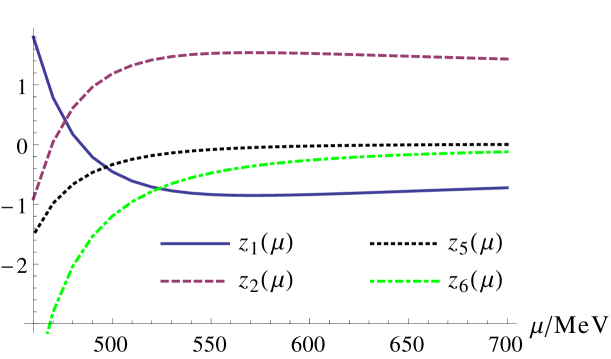
Figure 4: Wilson Coefficients, $z_{i}(\mu)$. The abscissa represents the energy scale, $\mu$, in units of MeV.

II.4 Coupling for the $K\sigma$ transition

With the Wilson coefficients and the NJL model explained, we can proceed with the calculation of the weak $K$ to $\sigma$ transition amplitude, $g_{K\sigma}$

$$g_{K\sigma}=\sqrt{2}\langle\sigma|\mathcal{H}_{\mbox{eff}}|K^{0}\rangle\,,$$ (22)

as illustrated in Fig. 5. Here we simply assume that the quarks appearing in the QCD operators $Q_{i}$ are the same as the NJL quark operators of the corresponding flavors with the energy scale $\mu$ lying in some region not yet accurately specified. Therefore, we first show our results for $\mu$ in the range 0.48$\sim$0.70 GeV and then use the numerical results to identify the optimal region. This is shown in Section V.

The corresponding matrix elements are evaluated with dimensional regularization using modified minimal subtraction in order to be consistent with the relevant Wilson coefficients, $z_{i}(\mu)$. We find that the contributions of $Q_{1}\sim Q_{4}$ to $g_{K\sigma}$ vanish, with only $Q_{5}$ and $Q_{6}$ contributing to $g_{K\sigma}$ in our results. In a more sophisticated model, where the masses of the constituent quarks and the couplings between the mesons and quark pairs were momentum dependent, the operators $Q_{1}$to $Q_{4}$ would also contribute to $g_{K\sigma}$. The full expressions for the $K\sigma$ transition amplitude are given in Appendix A.

Figure 5: Illustration of the $K\sigma$ transition, where the solid line with an $s$ represents $s$ quark and the other solid lines represent $u$ or $d$ quarks.

III Direct Decay to Pions

The second mechanism contributing to the decay $K\rightarrow\pi\,\pi$ proceeds directly to two pions, as illustrated in Fig. 6.

Figure 6: The possible diagrams for the direct weak decay. The solid line with $s$ represents $s$ quark, other solid line represents $u$ or $d$ quark. For the operator $Q_{1}$ and $Q_{2}$, only Fig. 6 contributes in the NJL model.

Since the Wilson coefficients $z_{1}$ and $z_{2}$ are much larger than others, we only consider the contributions of $Q_{1}$ and $Q_{2}$. Once again the diagrams are calculated with dimensional regularization and modified minimal subtraction. After calculation, we find that only Fig. 6 contributes to our results in the NJL model.

IV Final State Interaction

We denote the amplitudes corresponding to the diagrams shown in Figs. 1 and  6, without the contribution of the final state interaction, as $A_{I}^{0}$($A_{I}^{\sigma,0}$ and $A_{I}^{D,0}$). We must also consider the effect of final state interactions(FSI), which we treat using the method of Refs. Locher1997 ; Pallante2000

$$A_{I} = A_{I}^{0}\times F_{I}(m_{K}^{2})$$ (23)

$$\approx A_{I}^{0}\times\exp(\frac{m_{K}^{2}}{\pi}\int_{4m_{\pi}^{2}}^{\infty}\frac{\delta^{I}(s^{\prime})}{s^{\prime}(s^{\prime}-m_{K}^{2})}ds^{\prime})$$

$$\approx A_{I}^{0}\times\exp(\frac{m_{K}^{2}}{\pi}\int_{4m_{\pi}^{2}}^{\rm 1.0GeV}\frac{\delta^{I}(s^{\prime})}{s^{\prime}(s^{\prime}-m_{K}^{2})}ds^{\prime}),\qquad$$

where $\delta^{I}(s)$ is the phase shift for pion-pion scattering with isospin $I$ and we take the values of $\delta^{I}(s)$ from Ref. Dai2012 . This yields the result:

$$F_{0}(m_{K}^{2})\approx 1.4e^{i\,40{}^{\tiny o}},\quad F_{2}(m_{K}^{2})\approx 0.94e^{-i\,7.2{}^{\tiny o}}.$$ (24)

V Numerical Results and Discussion

As we have explained, in this work $A_{0}$ contains two contributions, the first, $A_{0}^{\sigma}$, involving the coupling to the $\sigma$ meson and the second, $A_{0}^{D}$, involving the direct decay to pions. Since, in the NJL model, $A_{0}^{\sigma}$ involves the weak operators $Q_{5}$ and $Q_{6}$, while $A_{0}^{D}$ involves $Q_{1}$ and $Q_{2}$, their contributions can be added with no worry about double counting $|A_{0}|=|A_{0}^{\sigma}|+|A_{0}^{D}|$.

We list the $K$-$\sigma$ coupling and the decay amplitudes with $m_{\sigma}=520,560,600~{}{\rm MeV}$, as a function of the matching scale, $\mu$, in Tables 2, 3, and 4. From these Tables one sees that the decay amplitudes are sensitive to both $\mu$ and $m_{\sigma}$.

Table 2: the $K$-$\sigma$ coupling and the decay amplitudes with $m_{\sigma}=520~{}{\rm MeV}$.

$\mu~{}(\rm{GeV})$	0.7	0.6	0.5	0.49	0.489	0.488	0.487	0.486	0.485	0.484	0.483	0.482
$|g_{K\sigma}|,~{}({\rm keV^{2}})$	703	1365	5184	6435	6584	6739	6898	7063	7233	7410	7592	7781
$|A_{0}^{\sigma}|~{}({\rm eV})$	22	42	159	197	201	206	211	216	221	226	232	237
$|A_{0}^{D}|~{}({\rm eV})$	79	73	54	49	48	48	47	46	46	45	44	44
$|A_{2}^{D}|~{}({\rm eV})$	37	37	26	20	19	18	17	16	15	14	13	11
$|A_{0}^{\sigma}|+|A_{0}^{D}|~{}({\rm eV})$	101	116	213	246	250	254	258	262	267	271	276	281
$(|A_{0}^{\sigma}|+|A_{0}^{D}|)/|A_{2}^{D}|$	2.7	3.1	8.1	13	13	14	15	16	18	20	22	25

Table 3: the $K$-$\sigma$ coupling and the decay amplitudes with $m_{\sigma}=560~{}{\rm MeV}$.

$\mu~{}(\rm{GeV})$	0.7	0.6	0.5	0.49	0.489	0.488	0.487	0.486	0.485	0.484	0.483	0.482
$|g_{K\sigma}|,~{}({\rm keV^{2}})$	1063	2031	7423	9096	9290	9489	9694	9903	10118	10337	10561	10789
$|A_{0}^{\sigma}|~{}({\rm eV})$	13	24	88	108	110	112	115	117	120	122	125	127
$|A_{0}^{D}|~{}({\rm eV})$	82	74	54	50	50	49	49	49	48	48	47	47
$|A_{2}^{D}|~{}({\rm eV})$	39	40	27	19	18	17	16	15	13	12	11	9.2
$|A_{0}^{\sigma}|+|A_{0}^{D}|~{}({\rm eV})$	94	99	143	158	160	162	164	166	168	170	172	174
$(|A_{0}^{\sigma}|+|A_{0}^{D}|)/|A_{2}^{D}|$	2.4	2.5	5.3	8.2	8.8	9.5	10	11	12	14	16	19

Table 4: the $K$-$\sigma$ coupling and the decay amplitudes with $m_{\sigma}=600~{}{\rm MeV}$.

$\mu~{}(\rm{GeV})$	0.7	0.6	0.5	0.49	0.489	0.488	0.487	0.486	0.485	0.484	0.483	0.482
$|g_{K\sigma}|,~{}({\rm keV^{2}})$	1457	2728	9312	10818	10902	10922	10736	10535	10783	11041	11310	11589
$|A_{0}^{\sigma}|~{}({\rm eV})$	11	21	72	83	84	84	83	81	83	85	87	89
$|A_{0}^{D}|~{}({\rm eV})$	83	75	54	52	52	52	52	52	52	52	52	52
$|A_{2}^{D}|~{}({\rm eV})$	41	42	28	18	17	16	14	12	11	9.1	7.3	5.5
$|A_{0}^{\sigma}|+|A_{0}^{D}|~{}({\rm eV})$	94	96	126	135	136	136	135	133	135	137	139	141
$(|A_{0}^{\sigma}|+|A_{0}^{D}|)/|A_{2}^{D}|$	2.3	2.3	4.5	7.4	8	8.7	9.6	11	13	15	19	26

In Refs. Buras2014 ; Buras2014b , the authors used the $\overline{\rm MOM}$ scheme to evolve the Wilson coefficients and hadronic matrix elements to the same energy scale. In order to match the energy scales, the Wilson coefficients were evolved from $\mu=O(M_{W})$ to $\mu=O(0.6\sim 1~{}{\rm GeV})$ in the quark-gluon picture, while the hadronic matrix elements were evolved from $\mu=O(m_{\pi})$ to the same scale $\mu=O(0.6\sim 1~{}{\rm GeV})$ in the meson picture. $|A_{0}|/|A_{2}|$ was found to lie in the range 12.5$\sim$14.9 as $\mu$ varied from 0.6$\sim$1 GeV, if only the contributions from $Q_{1}$ and $Q_{2}$ were included.

We notice that the $\mu$ dependence of their results was smaller than what we have found. Here both the hadronic matrix elements and the Wilson coefficients are evaluated with dimensional regularization and modified minimal subtraction. (As an extension of the present work it would be interesting to attempt to further reduce the $\mu$-dependence by including higher order loop corrections.) Within the present work, as in many other applications of valence dominated quark models, the model is assumed to represent QCD at a scale at which the gluons are effectively frozen out as degrees of freedom and valence quarks interacting through a chiral effective Lagrangian dominate the dynamics. Thus the best one can do is to match the scale of the effective weak Hamiltonian to the scale at which the NJL model best matches experiment, which seems to be around $0.4-0.5$ GeV.

We note that, in addition to the processes included here, there are also diagrams which are disconnected if the gluon lines are removed (usually just called disconnected diagrams for short). While such disconnected diagrams can contribute to $A_{0}$, they do not naturally appear within the NJL model and we omit them here. Since $A_{2}^{D}$ is not contributed by the disconnected diagrams, we use it to fix the energy scale $\mu$.

As we already noted earlier, in order that the evolution of the Wilson coefficients is under control, the matching scale, $\mu$, should not be lower than about 480 MeV. This creates some tension as the scale associated with the NJL model, when matching to phenomenological parton distribution functions, tends to be nearer 400-450 MeV. Fortunately, we see from Tables 2, 3 and 4 that if we choose $\mu$ to be in the range 0.484$\sim$0.488 GeV, $A_{2}^{D}$ (which does not involve the $\sigma$ meson) actually lies very close to its experimental value, 14.8 eV. We allow a small variation of $\mu$ for different values of $m_{\sigma}$ in order to calculate $A_{0}$. For $m_{\sigma}=520,560,600~{}{\rm MeV}$, we choose $\mu$ to be in the range 0.484$\sim$0.485 GeV, 0.485$\sim$0.486 GeV, and 0.487$\sim$0.488 GeV, respectively.

With $\mu$ fixed in the range where the empirical value of $A_{2}$ is reproduced, one notices that $|A_{0}|=|A_{0}^{\sigma}|+|A_{0}^{D}|$ lies in the range 135$\sim$270 eV, as $m_{\sigma}$ varies over the range 520$\sim$600 MeV. $A_{0}$ is close to the experimental value of 332 eV at $m_{\sigma}=520~{}{\rm MeV}$. From Tables 2, 3, and 4, we notice that $A_{0}^{\sigma}$ is sensitive to the choice of $m_{\sigma}$ because $A_{0}^{\sigma}\propto 1/(m_{K}-m_{\sigma})$, while $A_{0}^{D}$ and $A_{2}^{D}$ are not sensitive to it. $A_{0}^{\sigma}$ decreases as $m_{\sigma}$ moves away from $m_{K}$.

In view of the uncertainties in matching the model scale to the scale of the weak effective Hamiltonian, it is unrealistic to expect to obtain a prediction for the decay amplitudes. Nevertheless, our calculation clearly confirms that the $\sigma$ meson does indeed play an important role in $A_{0}$, since it contributes up to 65% of the final value, while the direct decay process contributes a mere 15%.

Appendix A expressions for the $K\sigma$ transition coupling

One can obtain the $K\sigma$ transition coupling $g_{K\sigma}$ with Eq. (15), Eq. (22) and the matrix elements of $Q_{i}$. The matrix elements of $Q_{1}$ to $Q_{4}$ vanish in NJL model, and those of $Q_{5}$ and $Q_{6}$ are expressed as

$$\langle\sigma|Q^{5}|K^{0}\rangle=\frac{1}{3}\langle\sigma|Q^{6}|K^{0}\rangle$$ (25)

$$= \sqrt{2}g_{K^{0}\bar{d}s}g_{\sigma\bar{q}q}\times$$

$$\left\{\right.48\left[(2m_{d}^{2}-p^{2})J^{F}_{0}(m_{d},m_{d},p^{2})+2p^{2}J^{F}_{21}(m_{d},m_{d},p^{2})+8J^{F}_{22}(m_{d},m_{d},p^{2})\right]$$

$$\quad\quad\times\left[m_{d}m_{s}J^{F}_{0}(m_{d},m_{s},p^{2})-p^{2}J^{F}_{11}(m_{d},m_{s},p^{2})-p^{2}J^{F}_{21}(m_{d},m_{s},p^{2})-4J^{F}_{22}(m_{d},m_{s},p^{2})\right]$$

$$+\frac{3}{2\pi^{2}}(6m_{d}^{2}-p^{2})\left[m_{d}m_{s}J^{F}_{0}(m_{d},m_{s},p^{2})-p^{2}J^{F}_{11}(m_{d},m_{s},p^{2})-p^{2}J^{F}_{21}(m_{d},m_{s},p^{2})-4J^{F}_{22}(m_{d},m_{s},p^{2})\right]$$

$$-\frac{3}{2\pi^{2}}(2m_{d}^{2}-2m_{d}m_{s}+2m_{s}^{2}-p^{2})$$

$$\quad\quad\times\left[m_{d}^{2}J^{F}_{0}(m_{d},m_{d},p^{2})+p^{2}J^{F}_{11}(m_{d},m_{d},p^{2})+p^{2}J^{F}_{21}(m_{d},m_{d},p^{2})+4J^{F}_{22}(m_{d},m_{d},p^{2})\right]$$

$$\left.\right\}.$$

The second and third terms in the brace will exist only with the dimension regularization, and they will vanish if using other regularization methods such as proper-time regularization. $J^{F}_{l}(m,M,p^{2})$ are defined by the following integrals

$$i\int\frac{d^{4}q}{(2\pi)^{4}}\frac{\{1,q^{\alpha},q^{\alpha}q^{\beta}\}}{[q^{2}-m^{2}+i\epsilon][(q-p)^{2}-M^{2}+i\epsilon]}$$ (26)

$$= \{J^{F}_{0},-p^{\alpha}J^{F}_{11},p^{\alpha}p^{\beta}J^{F}_{21}+g^{\alpha\beta}\frac{4}{D}J^{F}_{22}\}(m,M,p^{2}).$$

In the dimensional regularization, $J^{F}_{l}(m,M,p^{2})$ can be expressed as

$$J^{F}_{0}(m,M,p^{2}) = \frac{1}{16\pi^{2}}[2L+1+J^{i}_{1}(m,M,p^{2})],$$ (27)

$$J^{F}_{11}(m,M,p^{2}) = \frac{1}{2}[\frac{J^{i}_{0}(m)}{p^{2}}-\frac{J^{i}_{0}(M)}{p^{2}}-\frac{m^{2}-M^{2}+p^{2}}{p^{2}}J^{F}_{0}(m,M,p^{2})],$$ (28)

$$J^{F}_{21}(m,M,p^{2}) = \frac{1}{p^{2}}[J^{i}_{0}(M)+m^{2}J^{F}_{0}(m,M,p^{2})-4J^{F}_{22}(m,M,p^{2})],$$ (29)

$$J^{F}_{22}(m,M,p^{2}) = \frac{D}{4(D-1)}[J^{i}_{0}(M)+m^{2}J^{F}_{0}(m,M,p^{2})+\frac{m^{2}-M^{2}+p^{2}}{2}J^{F}_{11}(m,M,p^{2})-\frac{1}{2}J^{i}_{0}(M)],$$ (30)

and the definitions of the helping functions $J^{i}_{l}$ are

$$J^{i}_{0}(m) = \frac{m^{2}}{16\pi^{2}}(2L+\log\frac{m^{2}}{\mu^{2}}),$$ (31)

$$J^{i}_{1}(m,M,p^{2}) = -2+\ln|\frac{p^{2}}{\mu^{2}}|+X_{+}\ln|a+X_{+}^{2}|-X_{-}\ln|a+X_{-}^{2}|$$ (37)

$$+\left\{\begin{array}[]{ll}\displaystyle 2\sqrt{-a}({\rm arctanh}\frac{X_{+}}{\sqrt{-a}}-{\rm arctanh}\frac{X_{-}}{\sqrt{-a}})&~{}p^{2}<0\\ \displaystyle\sqrt{|a|}\ln Y&~{}0<p^{2}\leq(m-M)^{2}\\ \displaystyle 2\sqrt{a}(\arctan\frac{X_{+}}{\sqrt{a}}-\arctan\frac{X_{-}}{\sqrt{a}})&~{}(m-M)^{2}<p^{2}\leq(m+M)^{2}\\ \displaystyle\sqrt{|a|}\ln Y-2i\pi\sqrt{|a|}&~{}p^{2}>(m+M)^{2}\\ \end{array}\right.,$$

where

$$a = \frac{m^{2}}{p^{2}}-\frac{1}{4}(\frac{M^{2}}{p^{2}}-\frac{m^{2}}{p^{2}}-1)^{2},$$

$$X_{\pm} = \frac{1}{2}(\frac{M^{2}}{p^{2}}-\frac{m^{2}}{p^{2}}\pm 1),$$

$$Y = \left|\frac{1+X_{+}/\sqrt{|a|}}{1-X_{+}/\sqrt{|a|}}\frac{1-X_{-}/\sqrt{|a|}}{1+X_{-}/\sqrt{|a|}}\right|,$$

$$L = -\frac{1}{2}+\left[\frac{1}{D-4}+\frac{1}{2}(\gamma_{E}-\ln 4\pi)\right].$$ (38)

References

- (1) M. Gell-Mann and A. Pais, Phys. Rev. 97, 1387 (1955).
- (2) M. Gell-Mann and A. H. Rosenfeld, Ann.Rev.Nucl.Part.Sci. 7, 407 (1957).
- (3) P. A. Boyle, et al. (The RBC and UKQCD Collaborations), Phys. Rev. Lett. 110, 152001 (2013).
- (4) S. Bertolini, J. Eeg, M. Fabbrichesi, and E. Lashin, Nucl. Phys. B 514, 63 (1998).
- (5) J. Kambor, J. Missimer, and D. Wyler, Nucl. Phys. B 346, 17 (1990).
- (6) J. Kambor, J. Missimer, and D. Wyler, Phys. Lett. B 261, 496 (1991).
- (7) J. Kambor, J. F. Donoghue, B. R. Holstein, J. H. Missimer and D. Wyler, Phys. Rev. Lett. 68, 1818 (1992).
- (8) J. Bijnens and A. Celis, Phys. Lett. B 680, 466 (2009).
- (9) A. Buras, J.-M. Gérard, and W. Bardeen, Eur. Phys. J. C 74, 2871 (2014).
- (10) T. Hambye, G. Köhler, and P. Soldan, Eur. Phys. J. C 10, 271 (1999).
- (11) T. Hambye, S. Peris, and E. de Rafael, J. High Energy Phys. 2003, 027 (2003).
- (12) V. Cirigliano, G. Ecker, H. Neufeld, and A. Pich, Eur. Phys. J. C 33, 369 (2004).
- (13) J.-M. Gérard and J. Weyers, Phys. Lett. B 503, 99 (2001).
- (14) L. Giusti, et al., J. High Energy Phys. 2004, 016 (2004).
- (15) T. Hambye, B. Hassanain, J. March-Russell, and M. Schvellinger, Phys. Rev. D 74, 026003 (2006).
- (16) A. J. Buras, F. De Fazio, and J. Girrbach, arXiv: 1404.3824 (2014).
- (17) T. N. Truong, Phys. Lett. B 207, 495 (1988).
- (18) R. Crewther, Nucl. Phys. B 264, 277 (1986).
- (19) M. Shifman, A. Vainshtein, and V. Zakharov, Nucl. Phys. B 120, 316 (1977).
- (20) N. Carrasco, V. Lubicz, and L. Silvestrini, arXiv: 1312.6691 (2013).
- (21) A. J. Buras, arXiv: 1408.4820 (2014).
- (22) T. Blum, et al. (The RBC and UKQCD Collaborations), Phys. Rev. D 86, 074513 (2012).
- (23) T. Blum, et al. (RBC and UKQCD Collaborations), Phys. Rev. Lett. 108, 141601 (2012).
- (24) A. Bel’kov, G. Bohm, D. Ebert, and A. Lanyov, Phys. Lett. B 220, 459 (1989).
- (25) M. P. Locher, V. E. Markushin, and H. Q. Zheng, Phys. Rev. D 55, 2894 (1997).
- (26) E. Pallante and A. Pich, Nucl. Phys. B 592, 294 (2000).
- (27) E. Pallante and A. Pich, Phys. Rev. Lett. 84, 2568 (2000).
- (28) M. Büchler, G. Colangelo, J. Kambor, and F. Orellana, Phys. Lett. B 521, 29 (2001).
- (29) N. Isgur, K. Maltman, J. Weinstein, and T. Barnes, Phys. Rev. Lett. 64, 161 (1990).
- (30) G. Brown, J. Durso, M. Johnson, and J. Speth, Phys. Lett. B 238, 20 (1990).
- (31) R. Crewther and L. C. Tunstall, arXiv: 1312.3319 (2013).
- (32) R. Crewther and L. C. Tunstall, arXiv: 1203.1321 (2012).
- (33) R. J. Crewther and L. C. Tunstall, Mod. Phys. Lett. A 28, 1360010 (2013).
- (34) M. Harada, F. Sannino, and J. Schechter, Phys. Rev. D 54, 1991 (1996).
- (35) S. P. Klevansky, Rev. Mod. Phys. 64, 649 (1992).
- (36) U. Vogl and W. Weise, Progress in Particle and Nuclear Physics 27, 195 (1991).
- (37) Y. Ninomiya, W. Bentz and I. C. Cloët, arXiv:1406.7212 [nucl-th].
- (38) M. E. Carrillo-Serrano, I. C. Cloët and A. W. Thomas, arXiv:1409.1653 [nucl-th].
- (39) D. Ebert, T. Feldmann and H. Reinhardt, Phys. Lett. B 388, 154 (1996) [hep-ph/9608223].
- (40) G. Hellstern, R. Alkofer and H. Reinhardt, Nucl. Phys. A 625, 697 (1997) [hep-ph/9706551].
- (41) W. Bentz and A. W. Thomas, Nucl. Phys. A 696, 138 (2001) [nucl-th/0105022].
- (42) T. Hatsuda and T. Kunihiro, Prog. Theor. Phys. 74, 765 (1985).
- (43) T. Inagaki, D. Kimura and A. Kvinikhidze, Phys. Rev. D 77, 116004 (2008) [arXiv:0712.1336 [hep-ph]].
- (44) H. Mineo, W. Bentz, N. Ishii, A. W. Thomas and K. Yazaki, Nucl. Phys. A 735, 482 (2004) [nucl-th/0312097].
- (45) I. C. Cloet, W. Bentz and A. W. Thomas, Phys. Lett. B 621, 246 (2005) [hep-ph/0504229].
- (46) I. C. Cloet, W. Bentz and A. W. Thomas, Phys. Lett. B 642, 210 (2006) [nucl-th/0605061].
- (47) A. W. Schreiber, A. W. Thomas and J. T. Londergan, Phys. Rev. D 42, 2226 (1990).
- (48) D. Diakonov, V. Petrov, P. Pobylitsa, M. V. Polyakov and C. Weiss, Nucl. Phys. B 480, 341 (1996) [hep-ph/9606314].
- (49) G. Buchalla, A. J. Buras, and M. E. Lautenbacher, Rev. Mod. Phys. 68, 1125 (1996).
- (50) I. Caprini, G. Colangelo, and H. Leutwyler, Phys. Rev. Lett. 96, 132001 (2006).
- (51) L.-Y. Dai, X.-G. Wang, and H.-Q. Zheng, Commun. Theor. Phys. 57, 841 (2012).