Magging: maximin aggregation
for inhomogeneous large-scale data

Abstract

Large-scale data analysis poses both statistical and computational problems which need to be addressed simultaneously. A solution is often straightforward if the data are homogeneous: one can use classical ideas of subsampling and mean aggregation to get a computationally efficient solution with acceptable statistical accuracy, where the aggregation step simply averages the results obtained on distinct subsets of the data. However, if the data exhibit inhomogeneities (and typically they do), the same approach will be inadequate, as it will be unduly influenced by effects that are not persistent across all the data due to, for example, outliers or time-varying effects. We show that a tweak to the aggregation step can produce an estimator of effects which are common to all data, and hence interesting for interpretation and often leading to better prediction than pooled effects.

1 Introduction

‘Big data’ often refers to a large collection of observations and the associated computational issues in processing the data. Some of the new challenges from a statistical perspective include:

1. The analysis has to be computationally efficient while retaining statistical efficiency (Chandrasekaran and Jordan,, 2013, cf.).

2. The data are ‘dirty’: they contain outliers, shifting distributions, unbalanced designs, to mention a few.

There is also often the problem of dealing with data in real-time, which we add to the (broadly interpreted) first challenge of computational efficiency (Mahoney,, 2011, cf.).

We believe that many large-scale data are inherently inhomogeneous: that is, they are neither i.i.d. nor stationary observations from a distribution. Standard statistical models (e.g. linear or generalized linear models for regression or classification, Gaussian graphical models) fail to capture the inhomogeneity structure in the data. By ignoring it, prediction performance can become very poor and interpretation of model parameters might be completely wrong. Statistical approaches for dealing with inhomogeneous data include mixed effect models (Pinheiro and Bates,, 2000), mixture models (McLachlan and Peel,, 2004) and clusterwise regression models (DeSarbo and Cron,, 1988): while they are certainly valuable in their own right, they are typically computationally very cumbersome for large-scale data. We present here a framework and methodology which addresses the issue of inhomogeneous data while still being vastly more efficient to compute than fitting much more complicated models such as the ones mentioned above.

Subsampling and aggregation.

If we ignore the inhomogeneous part of the data for a moment, a simple approach to address the computational burden with large-scale data is based on (random) subsampling: construct groups ${\cal G}_{1},\ldots,{\cal G}_{G}$ with ${\cal G}_{g}\subset\{1,\ldots,n\}$, where $n$ denotes the sample size and $\{1,\ldots,n\}$ is the index set for the samples. The groups might be overlapping (i.e., ${\cal G}_{g}\cap{\cal G}_{g^{\prime}}\neq\emptyset$ for $g\neq g^{\prime}$) and do not necessarily cover the index space of samples $\{1,\ldots,n\}$. For every group ${\cal G}_{g}$, we compute an estimator (the output of an algorithm) $\hat{\theta}_{g}$ and these estimates are then aggregated to a single “overall” estimate $\hat{\theta}_{\mathrm{aggr}}$, which can be achieved in different ways.

If we divide the data into $G$ groups of approximately equal size and the computational complexity of the estimator scales for $n$ samples like $n^{\alpha}$ for some $\alpha>1$, then the subsampling-based approach above will typically yield a computational complexity which is a factor $G^{\alpha-1}$ faster than computing the estimator on all data, while often just incurring an insubstantial increase in statistical error. In addition, and importantly, effective parallel distributed computing is very easy to do and such subsampling-based algorithms are well-suited for computation with large-scale data.

Subsampling and aggregation can thus partially address the first challenge about feasible computation but fails for the second challenge about proper estimation and inference in presence of inhomogeneous data. We will show that a tweak to the aggregation step, which we call “maximin aggregation”, can often deal also with the second challenge by focusing on effects that are common to all data (and not just mere outliers or time-varying effects).

Bagging: aggregation by averaging.

In the context of homogeneous data, Breiman, 1996a showed good prediction performance in connection with mean or majority voting aggregation and tree algorithms for regression or classification, respectively. Bagging simply averages the individual estimators or predictions.

Stacking and convex aggregation.

Again in the context of homogeneous data, the following approaches have been advocated. Instead of assigning a uniform weight to each individual estimator as in Bagging, Wolpert, (1992) and Breiman, 1996b proposed to learn the optimal weights by optimizing on a new set of data. Convex aggregation for regression has been studied in Bunea et al., (2007) and has been proved to lead to to approximately equally good performance as the best member of the initial ensemble of estimators. But in fact, in practice, Bagging and stacking can exceed the best single estimator in the ensemble if the data are homogeneous.

Magging: convex maximin aggregation.

With inhomogeneous data, and in contrast to data being i.i.d. or stationary realizations from a distribution, the above schemes can be misleading as they give all data-points equal weight and can easily be misled by strong effects which are present in only small parts of the data and absent for all other data. We show that a different type of aggregation can still lead to consistent estimation of the effects which are common in all heterogeneous data, the so-called maximin effects (Meinshausen and Bühlmann,, 2014). The maximin aggregation, which we call Magging, is very simple and general and can easily be implemented for large-scale data.

2 Aggregation for regression estimators

We now give some more details for the various aggregation schemes in the context of linear regression models with an $n\times p$ predictor (design) matrix $X$, whose rows correspond to $n$ samples of the $p$-dimensional predictor variable, and with the $n$-dimensional response vector $Y\in\mathbb{R}^{n}$; at this point, we do not assume a true p-dimensional regression parameter, see also the model in (2). Suppose we have an ensemble of regression coefficient estimates $\hat{\theta}_{g}\in\mathbb{R}^{p}\ (g=1,\ldots,G)$, where each estimate has been obtained from the data in group ${\cal G}_{g}$, possibly in a computationally distributed fashion. The goal is to aggregate these estimators into a single estimator $\hat{\theta}_{\mathrm{aggr}}$.

2.1 Mean aggregation and Bagging

Bagging (Breiman, 1996a, ) simply averages the ensemble members with equal weight to get the aggregated estimator

$$\mbox{\bf Mean aggregation:}\quad\hat{\theta}_{\mathrm{aggr}} :=\sum_{g=1}^{G}w_{g}\hat{\theta}_{g},$$

$$\mbox{where }w_{g}=\frac{1}{G}\mbox{ for all }g=1,\ldots,G.$$

One could equally average the predictions $X\hat{\theta}_{g}$ to obtain the predictions $X\hat{\theta}_{\mathrm{aggr}}$. The advantage of Bagging is the simplicity of the procedure, its variance reduction property (Bühlmann and Yu,, 2002), and the fact that it is not making use of the data, which allows simple evaluation of its performance. The term “Bagging” stands for Bootstrap aggregating (mean aggregation) where the ensemble members $\hat{\theta}_{g}$ are fitted on bootstrap samples of the data, that is, the groups ${\cal G}_{g}$ are sampled with replacement from the whole data.

2.2 Stacking

Wolpert, (1992) and Breiman, 1996b propose the idea of “stacking” estimators. The general idea is in our context as follows. Let $\hat{Y}(g)=X\hat{\theta}_{g}\in\mathbb{R}^{n}$ be the prediction of the $g$-th member in the ensemble. Then the stacked estimator is found as

$$\mbox{\bf Stacked aggregation:}\quad\hat{\theta}_{\mathrm{aggr}} :=\sum_{g=1}^{G}w_{g}\hat{\theta}_{g},$$

$$\mbox{where }w :=\mbox{argmin}_{w\in W}\|Y-\sum_{g}\hat{Y}(g)w_{g}\|_{2},$$

where the space of possible weight vectors is typically of one of the following forms:

(ridge constraint) $$:W=\{w:\|w\|_{2}\leq s\}\mbox{ for some }s>0$$

(sign constraint) $$:W=\{w:\min_{g}w_{g}\geq 0\}$$

(convex constraint) $$:W=\{w:\min_{g}w_{g}\geq 0\mbox{ and }\sum_{g}w_{g}=1\}$$

If the ensemble of initial estimators $\hat{\theta}_{g}\ (g=1,\ldots,G)$ is derived from an independent dataset, the framework of stacked regression has also been analyzed in Bunea et al., (2007). Typically, though, the groups on which the ensemble members are derived use the same underlying dataset as the aggregation. Then, the predictions $\hat{Y}(g)$ are for each sample point $i=1,\ldots,n$ defined as being generated with $\hat{\theta}_{g}^{(-i)}$, which is the same estimator as $\hat{\theta}_{g}$ with observation $i$ left out of group ${\cal G}_{g}$ (and consequently $\hat{\theta}_{g}^{(-i)}=\hat{\theta}_{g}$ if $i\notin{\cal G}_{g}$). Instead of a leave-one-out procedure, one could also use other leave-out schemes, such as e.g. the out-of-bag method (Breiman,, 2001). To this end, we just average for a given sample over all estimators that did not use this sample point in their construction, effectively setting $\hat{\theta}_{g}^{(-i)}\equiv 0$ if $i\in{\cal G}_{g}$. The idea of “stacking” is thus to find the optimal linear or convex combination of all ensemble members. The optimization is $G$-dimensional and is a quadratic programming problem with linear inequality constraints, which can be solved efficiently with a general-purpose quadratic programming solver. Note that only the inner products $\hat{Y}(g)^{t}\hat{Y}_{g^{\prime}}$ and $\hat{Y}(g)^{t}Y$ for $g,g^{\prime}\in\{1,\ldots,G\}$ are necessary for the optimization.

Whether stacking or simple mean averaging as in Bagging provides superior performance depends on a range of factors. Mean averaging, as in Bagging, certainly has an advantage in terms of simplicity. Both schemes are, however, questionable when the data are inhomogeneous. It is then not evident why the estimators should carry equal aggregation weight (as in Bagging) or why the fit should be assessed by weighing each observation identically in the squared error loss sense (as in stacked aggregation).

2.3 Magging: maximin aggregation for heterogeneous data

We propose here Maximin aggregating, called Magging, for heterogeneous data: the concept of maximin estimation has been proposed by Meinshausen and Bühlmann, (2014), and we present a connection in Section 3. The differences and similarities to mean and stacked aggregation are:

1. The aggregation is a weighted average of the ensemble members (as in both stacked aggregation and Bagging).

2. The weights are non-uniform in general (as in stacked aggregation).

3. The weights do not depend on the response $Y$ (as in Bagging).

The last property makes the scheme almost as simple as mean aggregation as we do not have to develop elaborate leave-out schemes for estimation (as in e.g. stacked regression). Magging is choosing the weights as a convex combination to minimize the $\ell_{2}$-norm of the fitted values:

$$\mbox{\bf Magging:}\quad\hat{\theta}_{\mathrm{aggr}} :=\sum_{g=1}^{G}w_{g}\hat{\theta}_{g},$$

$$\mbox{where }w :=\mbox{argmin}_{w\in C_{G}}\|\sum_{g}\hat{Y}(g)w_{g}\|_{2},$$ (1)

$$\mbox{and }C_{G} :=\{w:\min_{g}w_{g}\geq 0\mbox{ and }\sum_{g}w_{g}=1\}.$$

If the solution is not unique, we take the solution with lowest $\ell_{2}$-norm of the weight vector among all solutions.

The optimization and computation can be implemented in a very efficient way. The estimators $\hat{\theta}_{g}$ are computed in each group of data ${\cal G}_{g}$ separately, and this task can be easily performed in parallel. In the end, the estimators only need to be combined by calculating optimal convex weights in $G$-dimensional space (where typically $G\ll n$ and $G\ll p$) with quadratic programming; some pseudocode in R (R Core Team,, 2014) for these convex weights is presented in the Appendix. Computation of Magging is thus computationally often massively faster and simpler than a related direct estimation estimation scheme proposed in Meinshausen and Bühlmann, (2014). Furthermore, Magging is very generic (e.g. one can choose its own favored regression estimator $\hat{\theta}_{g}$ for the $g$-th group) and also straightforward to use in more general settings beyond linear models.

The Magging scheme will be motivated in the following Section 3 with a model for inhomogeneous data and it will be shown that it corresponds to maximizing the minimally “explained variance” among all data groups. The main idea is that if an effect is common across all groups ${\cal G}_{g}\ (g=1,\ldots,G)$, then we cannot “average it away” by searching for a specific convex combination of the weights. The common effects will be present in all groups and will thus be retained even after the minimization of the aggregation scheme.

The construction of the groups ${\cal G}_{g}\ (g=1,\ldots,G)$ for Magging in presence of inhomogeneous data is rather specific and described in Section 3.3.1 for various scenarios. There, Examples 1 and 2 represent the setting where the data within each group is (approximately) homogeneous, whereas Example 3 is a case with randomly subsampled groups, despite the fact of inhomogeneity in the data.

3 Inhomogeneous data and maximin effects

We motivate in the following why Magging (maximin aggregation) can be useful for inhomogeneous data when the interest is on effects that are present in all groups of data.

In the linear model setting, we consider the framework of a mixture model

$$Y_{i}=X_{i}^{t}B_{i}+\varepsilon_{i},\ i=1,\ldots,n,$$ (2)

where $Y_{i}$ is a univariate response variable, $X_{i}$ is a $p$-dimensional covariable, $B_{i}$ is a $p$-dimensional regression parameter, and $\varepsilon_{i}$ is a stochastic noise term with mean zero and which is independent of the (fixed or random) covariable. Every sample point $i$ is allowed to have its own and different regression parameter: hence, the inhomogeneity occurs because of changing parameter vectors, and we have a mixture model where, in principle, every sample arises from a different mixture component. The model in (2) is often too general: we make the assumption that the regression parameters $B_{1},\ldots,B_{n}$ are realizations from a distribution $F_{B}$:

$$B_{i}\sim F_{B},\ i=1,\ldots,n,$$ (3)

where the $B_{i}$’s do not need to be independent of each other. However, we assume that the $B_{i}$’s are independent from the $X_{i}$’s and $\varepsilon_{i}$’s.

Example 1: known groups. Consider the case where there are known groups ${\cal G}_{g}$ with $B_{i}\equiv b_{g}$ for all $i\in{\cal G}_{g}$. Thus, this is a clusterwise regression problem (with known clusters) where every group ${\cal G}_{g}$ has the same (unknown) regression parameter vector $b_{g}$. We note that the groups ${\cal G}_{g}$ are the ones for constructing the Magging estimator described in the previous section.

Example 2: smoothness structure. Consider the situation where there is a smoothly changing behavior of the $B_{i}$’s with respect to the sample indices $i$: this can be achieved by positive correlation among the $B_{i}$’s. In practice, the sample index often corresponds to time. There are no true (unknown) groups in this setting.

Example 3: unknown groups. This is the same setting as in Example 1 but the groups ${\cal G}_{g}$ are unknown. From an estimation point of view, there is a substantial difference to Example 1 (Meinshausen and Bühlmann,, 2014).

3.1 Maximin effects

In model (2) and in the Examples 1–3 mentioned above, we have a “multitude” of regression parameters. We aim for a single $p$-dimensional parameter, which contains the common components among all $B_{i}$’s (and essentially sets the non-common components to the value zero). This can be done by the idea of so-called maximin effects which we explain next.

Consider a linear model with the fixed $p$-dimensional regression parameter $b$ which can take values in the support of $F_{B}$ from (3):

$$Y_{i}=X_{i}^{t}b+\varepsilon_{i},\ i=1,\ldots,n,$$ (4)

where $X_{i}$ and $\varepsilon_{i}$ are as in (2) and assumed to be i.i.d. We will connect the random variables $B_{i}$ in (2) to the values $b$ via a worst-case analysis as described below: for that purpose, the parameter $b$ is assumed to not depend on the sample index $i$. The variance which is explained by choosing a parameter vector $\beta$ in the linear model (4) is

$$V_{\beta,b}:=\mathbb{E}|Y|^{2}-\mathbb{E}|Y-X^{t}\beta|^{2}=2\beta^{t}\Sigma b-\beta^{t}\Sigma\beta,$$

where $\Sigma$ denotes the covariance matrix of $X$. We aim for maximizing the explained variance in the worst (most adversarial) scenario: this is the definition of the maximin effects.

Definition (Meinshausen and Bühlmann,, 2014). The maximin effects parameter is

$$b_{\mathrm{maximin}}=\mathrm{argmin}_{\beta}\max_{b\in\mathrm{supp}(F_{B})}-V_{\beta,b},$$

and note that the definition uses the negative explained variance $-V_{\beta,b}$.

The maximin effects can be interpreted as an aggregation among the support points of $F_{B}$ to a single parameter vector, i.e., among all the $B_{i}$’s (e.g. in Example 2) or among all the clustered values $b_{g}$ (e.g. in Examples 1 and 3), see also Fact 1 below. The maximin effects parameter is different from the pooled effects $b_{\mathrm{pool}}=\mathrm{argmin}_{\beta}\;\mathbb{E}_{B}[-V_{\beta,B}]$ and a bit surprisingly, also rather different from the prediction analogue

$$b_{\mathrm{pred-maximin}}=\mathrm{argmin}_{\beta}\max_{b\in\mathrm{supp}(F_{B})}\mathbb{E}[(X^{t}b-X^{t}\beta)^{2}].$$

In particular, the value zero has a special status for the maximin effects parameter $b_{\mathrm{maximin}}$, unlike for $b_{\mathrm{pred-maximin}}$ or $b_{\mathrm{pool}}$, see Meinshausen and Bühlmann, (2014). The following is an important “geometric” characterization which indicates the special status of the value zero, see also Figure 1.

Fact 1.

(Meinshausen and Bühlmann,, 2014) Let $H$ be the convex hull of the support of $F_{B}$. Then

$$b_{\mathrm{maximin}}=\mathrm{argmin}_{\gamma\in H}\;\gamma^{t}\Sigma\gamma.$$

That is, the maximin effects parameter $b_{\mathrm{maximin}}$ is the point in the convex hull $H$ which is closest to zero with respect to the distance $d(u,v)=(u-v)^{t}\Sigma(u-v)$: in particular, if the value zero is in $H$, the maximin effects parameter equals $b_{\mathrm{maximin}}\equiv 0$.

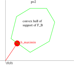
Figure 1: Illustration of Fact 1 in dimension $p=2$.

The characterization in Fact 1 leads to an interesting robustness issue which we will discuss below in Section 3.2.

The connection to Magging (maximin aggregation) can be made most easily for the setting of Example 1 with known groups and constant regression parameter $b_{g}$ within each group ${\cal G}_{g}$. We can rewrite, using Fact 1:

$$b_{\mathrm{maximin}}=\sum_{g=1}^{G}w_{g}^{0}b_{g},$$

$$w^{0}=(w_{1}^{0},\ldots,w_{G}^{0})=\mathrm{argmin}_{w\in C_{G}}\sum_{g,g^{\prime}=1}^{G}w_{g}w_{g^{\prime}}b_{g}^{T}\Sigma b_{g}=\mathrm{argmin}_{w\in C_{G}}\mathbb{E}_{X}\|\sum_{g=1}^{G}w_{g}Xb_{g}\|_{2}^{2},$$

where $C_{G}$ is as in (1). The Magging estimator is then using the plug-in principle with estimates $\hat{\theta}_{g}$ for $b_{g}$ and $\|\sum_{g}w_{g}\hat{Y}(g)\|_{2}^{2}$ for $\mathbb{E}_{X}\|\sum_{g=1}^{G}w_{g}Xb_{g}\|_{2}^{2}$.

3.2 Robustness

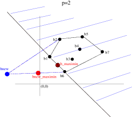
Figure 2: Illustration of the case with a finite number of possible values for $B$. Left panel: The values $b_{1},\ldots,b_{7}$ are possible realizations of $B_{i}$, and $b_{\mathrm{maximin}}$ is the closest point to zero in the convex hull of $\{b_{1},\ldots,b_{7}\}$ (in black). When adding a new additional realization $b_{\mathrm{new}}$, the convex hull becomes larger (in dashed blue). As long as the new support point is in the blue shaded half-space, the maximin effects parameter $b_{\mathrm{maximin}}$ remains the same regardless of how far away the new support point is added. Right panel: A new additional realization $b_{\mathrm{new}}$ arises which does not lie in the blue shaded half-space, the convex hull becomes larger (in dashed blue) and the new maximin effects parameter becomes $b_{\mathrm{new,maximin}}$. Since the new convex hull (in dashed blue) gets enlarged by a new realized value $b_{\mathrm{new}}$ , the corresponding new maximin effects parameter $b_{\mathrm{new,maximin}}$ must be closer to the origin than the original parameter $b_{\mathrm{maximin}}$. Thus, it is impossible to shift $b_{\mathrm{maximin}}$ away from zero by placing new realizations at arbitrary positions.

It is instructive to see how the maximin effects parameter is changing if the support of $F_{B}$ is extended, possibly rendering the support non-finite. There are two possibilities, illustrated by Figure 2. In the first case, illustrated in the left panel of Figure 2, the new parameter vector $b_{\mathrm{new}}$ is not changing the point in the convex hull of the support of $F_{B}$ that is closest to the origin. The maximin effects parameter is then unchanged. The second situation is illustrated in the right panel of Figure 2. The addition of a new support point here does change the convex hull of the support such that there is now a point in the support closer to the origin. Consequently, the maximin effects parameter will shift to this new value. The maximin effects parameter thus is either unchanged or is moving closer to the origin. Therefore, maximin effects parameters and their estimation exhibit an excellent robustness feature with respect to breakdown properties.

3.3 Statistical properties of Magging

We will derive now some statistical properties of Magging, the maximin aggregation scheme, proposed in (1). They depend also on the setting-specific construction of the groups ${\cal G}_{1},\ldots{\cal G}_{G}$ which is described in Section 3.3.1.

Assumptions.

Consider the model (2) and that there are $G$ groups ${\cal G}_{g}\ (g=1,\ldots,G)$ of data samples. Denote by $Y_{g}$ and $X_{g}$ the data values corresponding to group ${\cal G}_{g}$.

(A1)

Let $b^{*}_{g}$ be the optimal regression vector in each group, that is $b_{g}^{*}=\mathbb{E}_{B}[|{\cal G}_{g}|^{-1}\sum_{i\in{\cal G}_{g}}B_{i}]$. Assume that $b_{\mathrm{maximin}}$ is in the convex hull of $\{b^{*}_{1},\ldots,b^{*}_{G}\}$.

(A2)

We assume random design with a mean-zero random predictor variable $X$ with covariance matrix $\Sigma$ and let $\hat{\Sigma}_{g}=|{\cal G}_{g}|^{-1}X_{g}^{t}X_{g}$ be the empirical Gram matrices. Let $\hat{\theta}_{g}\ (g=1,\ldots,G)$ be the estimates in each group. Assume that there exists some $\eta_{1},\eta_{2}>0$ such that

$$\max_{g}(\hat{\theta}_{g}-b^{*}_{g})^{t}\Sigma(\hat{\theta}_{g}-b^{*}_{g}) \leq\eta_{1},$$

$$\max_{g}\|\hat{\Sigma}_{g}-\Sigma\|_{\infty} \leq\eta_{2},$$

where $m=\min_{g}|{\cal G}_{g}|$ is the minimal sample size across all groups.

(A3)

The optimal and estimated vectors are sparse in the sense that there exists some $\kappa>0$ such that

$$\max_{g}\|b^{*}_{g}\|_{1}\leq\kappa\quad\mbox{ and }\quad\max_{g}\|\hat{\theta}_{g}\|_{1}\leq\kappa.$$

Assumption (A1) is fulfilled for known groups, where the convex hull of $\{b^{*}_{1},\ldots,b^{*}_{G}\}$ is equal to the convex hull of the support of $F_{B}$ and the maximin-vector $b_{\mathrm{maximin}}$ is hence contained in the former. Example 1 is fulfilling the requirement, and we will discuss generalizations to the settings in Examples 2 and 3 below in Section 3.3.1. Assumptions (A2) and (A3) are relatively mild: the first part of (A3) is an assumption that the underlying model is sufficiently sparse. If we consider standard Lasso estimation with sparse optimal coefficient vectors and assuming bounded predictor variables, then (A2) is fulfilled with high probability for $\eta_{1}$ of the order $\kappa(\log(pG)/m)^{1/2}$ (faster rates are possible under a compatibility assumption) and $\eta_{2}$ of order $\log(pG)/m$, where $m=\min_{g}|{\cal G}_{g}|$ denotes the minimal sample size across all groups; see for see for example Meinshausen and Bühlmann, (2014).

Define for $x\in\mathbb{R}^{p}$, the norm $\|x\|_{\Sigma}^{2}=x^{t}\Sigma x$ and let $\hat{\theta}_{\mathrm{Magging}}$ be the Magging estimator (1).

Theorem 1.

Assume (A1)-(A3). Then

$$\|\hat{\theta}_{\mathrm{Magging}}-b_{\mathrm{maximin}}\|_{\Sigma}^{2}\;\leq\;6\eta_{1}+4\eta_{2}\kappa^{2}.$$

A proof is given in the Appendix.

The result implies that the maximin effects parameter can be estimated with good accuracy by Magging (maximin aggregation) if the individual effects in each group can be estimated accurately with standard methodology (e.g. penalized regression methods).

3.3.1 Construction of groups and their validity for different settings

Theorem 1 hinges mainly on assumption (A1). We discuss the validity of the assumption for the three discussed settings under appropriate (and setting-specific) sampling of the data-groups.

Example 1: known groups (continued). Obviously, the groups ${\cal G}_{g}\ (g=1,\ldots,G)$ are chosen to be the true known groups.

Assumption (A1) is then trivially fulfilled with known groups and constant regression parameter within groups (clusterwise regression).

Example 2: smoothness structure (continued). We construct $G$ groups of non-overlapping consecutive observations. For simplicity, we would typically use equal group size $m=\lfloor n/G\rfloor$ so that ${\cal G}_{1}=\{1,2,\ldots,m\},{\cal G}_{2}=\{m+1,\ldots,2m\},\ldots,{\cal G}_{G}=\{(G-1)m+1,\ldots,n\}$.

When taking sufficiently many groups and for a certain model of smoothness structure, condition (A1) will be fulfilled with high probability (Meinshausen and Bühlmann,, 2014): it is shown there that it is rather likely to get some groups of consecutive observations where the optimal vector is approximately constant and the convex hull of these “pure” groups will be equal to the convex hull of the support of $F_{B}$.

Example 3: unknown groups (continued). We construct $G$ groups of equal size $m$ by random subsampling: sample without replacement within a group and with replacement between groups.

This random subsampling strategy can be shown to fulfill condition (A1) when assuming an additional so-called Pareto condition (Meinshausen and Bühlmann,, 2014). As an example, a model with a fraction of outliers fulfills (A1) and one obtains an important robustness property of Magging which is closely connected to Section 3.2.

3.4 Numerical example

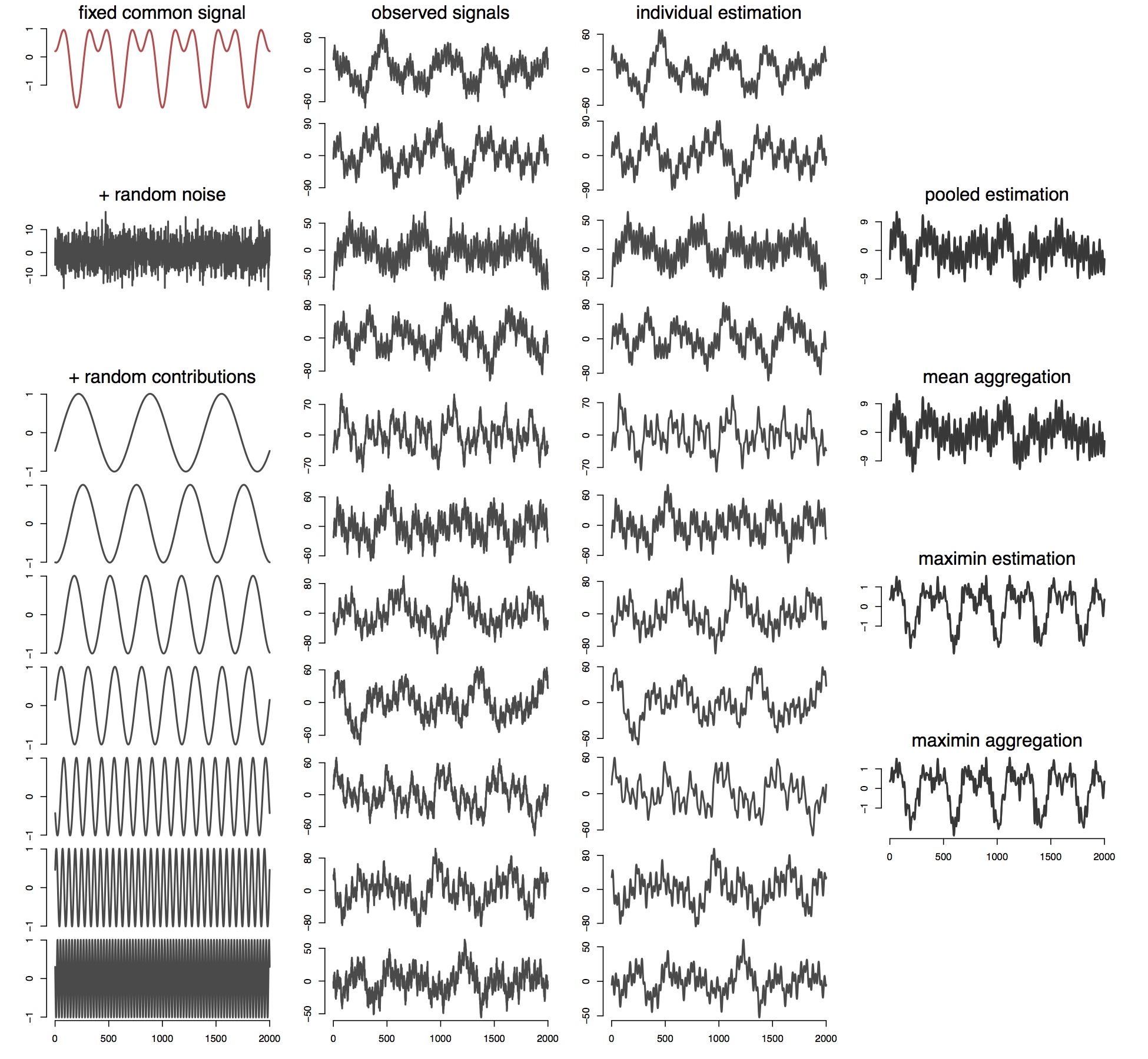
Figure 3: The left column shows the data generation. Each group has the same fixed common effect (shown in red at the top left), and gets random noise as well as other random periodic contributions added (with random phase), where the latter two contributions are drawn independently for all groups $g=1,\ldots,G=50$. The second column shows the realizations of $Y_{g}$ for the first groups $g=1,\ldots,11$, while the third shows the least-squares estimates of the signal when projecting onto the space of periodic signals in a certain frequency-range. The last column shows from top to bottom: (a) the pooled estimate one obtains when adding all groups into one large dataset and estimating the signal on all data simultaneously (the estimate does not match closely the common effects shown in red); (b) the mean aggregated data obtained by averaging the individual estimates (here identical to pooled estimation); (c) the (less generic) maximin effects estimator from Meinshausen and Bühlmann, (2014), and (d) Magging: maximin aggregated estimators (1), both of which match the common effects quite closely.

We illustrate the difference between mean aggregation and maximin aggregation (Magging) with a simple example. We are recording, several times, data in a time-domain. Each recording (or group of observations) contains a common signal, a combination of two frequency components, shown in the top left of Figure 3. On top of the common signal, seven out of a total of 100 possible frequencies (bottom left in Figure 3) add to the recording in each group with a random phase. The 100 possible frequencies are the first frequencies $2\pi j/P$, $j=1,\ldots,100$ for periodic signal with periodicity $P$ defined by the length of the recordings. They form the dictionary used for estimation of the signal. In total $G=50$ recordings are made, of which the first 11 are shown in the second column of Figure 3. The estimated signals are shown in the third column, removing most of the noise but leaving the random contribution from the non-common signal in place. Averaging over all estimates in the mean sense yields little resemblance with the common effects. The same holds true if we estimate the coefficients by pooling all data into a single group (first two panels in the rightmost column of Figure 3). Magging (maximin aggregation) and the closely related but less generic maximin estimation (Meinshausen and Bühlmann,, 2014), on the other hand, approximate the common signal in all groups quite well (bottom two panels in the rightmost column of Figure 3).

Meinshausen and Bühlmann, (2014) provide other real data results where maximin effects estimation leads to better out-of-sample predictions in two financial applications.

4 Conclusions

Large-scale and ‘Big’ data poses many challenges from a statistical perspective. One of them is to develop algorithms and methods that retain optimal or reasonably good statistical properties while being computationally cheap to compute. Another is to deal with inhomogeneous data which might contain outliers, shifts in distributions and other effects that do not fall into the classical framework of identically distributed or stationary observations. Here we have shown how Magging (“maximin aggregation”) can be a useful approach addressing both of the two challenges. The whole task is split into several smaller datasets (groups), which can be processed trivially in parallel. The standard solution is then to average the results from all tasks, which we call “mean aggregation” here. In contrast, we show that finding a certain convex combination, we can detect the signals which are common in all subgroups of the data. While “mean aggregation” is easily confused by signals that shift over time or which are not present in all groups, Magging (“maximin aggregation”) eliminates as much as possible these inhomogeneous effects and just retains the common signals which is an interesting feature in its own right and often improves out-of-sample prediction performance.

Appendix

Proof of Theorem 1: Define for $w\in C_{G}$ (where $C_{G}\subset\mathbb{R}^{G}$ is as defined in (1) the set of positive vectors that sum to one),

$$\hat{\theta}(w):=\sum_{g=1}^{G}w_{g}\hat{\theta}_{g}\quad\mbox{ and }\quad\theta(w):=\sum_{g=1}^{G}w_{g}b^{*}_{g}$$

And let for $\hat{\Sigma}=n^{-1}X^{t}X$,

$$\hat{L}(w):=\hat{\theta}(w)^{t}\hat{\Sigma}\hat{\theta}(w)\quad\mbox{ and }\quad L(w):=\theta(w)^{t}\Sigma\theta(w).$$

Then $w^{*}=\mathrm{argmin}_{w}L(w)$ and $b_{\mathrm{maximin}}=\theta(w^{*})$ and $\hat{w}=\mathrm{argmin}_{w}\hat{L}(w)$ and $\hat{\theta}_{\mathrm{Magging}}=\hat{\theta}(\hat{w})$. Now, using (A3)

$$\sup_{w\in C_{G}}|\hat{L}(w)-L(w)| \leq\sup_{w\in C_{G}}|\theta(w)^{t}(\Sigma-\hat{\Sigma})\theta(w)|+\max_{g}\|b^{*}_{g}-\hat{b}_{g}\|_{\Sigma}^{2}$$

$$\leq\eta_{2}(\max_{w\in C_{G}}\|\theta(w)\|_{1})^{2}+\eta_{1}.$$

Hence, as $w^{*}=\mathrm{argmin}_{w\in C_{G}}L(w)$ and $\hat{w}=\mathrm{argmin}_{w}\hat{L}(w)$,

$$L(\hat{w})\leq L(w^{*})+2(\eta_{1}+\eta_{2}\kappa^{2}).$$ (5)

For $\Delta:=\theta(\hat{w})-\theta(w^{*})$,

$$L(\hat{w})=\|\theta(\hat{w})\|_{\Sigma}^{2} =(\theta(w^{*})+\Delta)^{t}\Sigma(\theta(w^{*})+\Delta)$$

$$=\theta(w^{*})^{t}\Sigma\theta(w^{*})+2\Delta^{t}\Sigma\theta(w^{*})+\Delta^{t}\Sigma\Delta$$

$$\geq L(w^{*})+\|\Delta\|_{\Sigma}^{2},$$

where $\Delta^{t}\Sigma\theta(w^{*})\geq 0$ follows by the definition of the maximin vector $\theta(w^{*})=b_{\mathrm{maximin}}$. Combining the last inequality with (5),

$$\|\theta(\hat{w})-\theta(w^{*})\|_{\Sigma}^{2}\leq 2(\eta_{1}+\eta_{2}\kappa^{2})$$ (6)

Furthermore, by (A3),

$$\sup_{w\in C_{G}}\|\hat{\theta}(w)-\theta(w)\|_{\Sigma}^{2}\leq\eta_{1}.$$

Using the equality for $\hat{\theta}_{\mathrm{Magging}}=\hat{\theta}(\hat{w})$,

$$\|\hat{\theta}(\hat{w})-\theta(\hat{w})\|_{\Sigma}^{2}\leq\eta_{1}.$$ (7)

Combining (6) and (7),

$$\|\hat{\theta}_{\mathrm{Magging}}-b_{\mathrm{maximin}}\|_{\Sigma}^{2}=\|\hat{\theta}(\hat{w})-\theta(w^{*})\|_{\Sigma}^{2} \leq 2\big{(}\|\hat{\theta}(\hat{w})-\theta(\hat{w})\|_{\Sigma}^{2}+\|\theta(\hat{w})-\theta(w^{*})\|_{\Sigma}^{2}\big{)}$$

$$\leq 2\big{(}\eta_{1}+2(\eta_{1}+\eta_{2}\kappa^{2})\big{)}$$

$$=6\eta_{1}+4\eta_{2}\kappa^{2},$$

which completes the proof. $\Box$

Implementation of Magging in R:
We present here some pseudo-code for computing the weights $w_{1},\ldots,w_{G}$ in Magging (1), using quadratic programming in the R-software environment.

library(quadprog)
theta <- cbind(theta1,...,thetaG)   #matrix with G columns:
                                    #each column is a regression estimate

hatS <- t(X) %*% X/n                #empirical covariance matrix of X
H <- t(theta) %*% hatS %*% theta    #assume that it is positive definite
                                    #(use H + xi * I, xi > 0 small, otherwise)
A <- rbind(rep(1,G),diag(1,G))      #constraints
b <- c(1,rep(0,G))
d <- rep(0,G)                       #linear term is zero
w <- solve.QP(H,d,t(A),b, meq = 1)  #quadratic programming solution to
                                    #argmin(x^t H x) such that Ax >= b and
                                    #first inequality is an equality

References

- (1) Breiman, L. (1996a). Bagging predictors. Machine Learning, 24:123–140.
- (2) Breiman, L. (1996b). Stacked regressions. Machine Learning, 24:49–64.
- Breiman, (2001) Breiman, L. (2001). Random Forests. Machine Learning, 45:5–32.
- Bühlmann and Yu, (2002) Bühlmann, P. and Yu, B. (2002). Analyzing bagging. The Annals of Statistics, 30:927–961.
- Bunea et al., (2007) Bunea, B., Tsybakov, A., and Wegkamp, M. (2007). Aggregation for Gaussian regression. The Annals of Statistics, 35:1674–1697.
- Chandrasekaran and Jordan, (2013) Chandrasekaran, V. and Jordan, M. I. (2013). Computational and statistical tradeoffs via convex relaxation. Proceedings of the National Academy of Sciences, 110:E1181–E1190.
- DeSarbo and Cron, (1988) DeSarbo, W. and Cron, W. (1988). A maximum likelihood methodology for clusterwise linear regression. Journal of Classification, 5:249–282.
- Mahoney, (2011) Mahoney, M. W. (2011). Randomized algorithms for matrices and data. Foundations and Trends® in Machine Learning, 3:123–224.
- McLachlan and Peel, (2004) McLachlan, G. and Peel, D. (2004). Finite Mixture Models. John Wiley & Sons.