hep-ph/***

FTUAM-14-29 IFT-UAM/CSIC-14-071

DFPD2014/TH/15

On the renormalization of the electroweak
chiral Lagrangian with a Higgs

M.B. Gavela ^a) K. Kanshin ^b), P. A. N. Machado ^a), S. Saa ^a)

^a)  Departamento de Física Teórica and Instituto de Física Teórica, IFT-UAM/CSIC,
Universidad Autónoma de Madrid, Cantoblanco, 28049, Madrid, Spain
^b)  Dipartimento di Fisica e Astronomia “G. Galilei”, Università di Padova and
INFN, Sezione di Padova, Via Marzolo 8, I-35131 Padua, Italy E-mail: belen.gavela@uam.es kanshin@pd.infn.it, sara.saa@uam.es, pedro.machado@uam.es

We consider the scalar sector of the effective non-linear electroweak Lagrangian with a light “Higgs” particle, up to four derivatives in the chiral expansion. The complete off-shell renormalization procedure is implemented, including one loop corrections stemming from the leading two-derivative terms, for finite Higgs mass. This determines the complete set of independent chiral invariant scalar counterterms required for consistency; these include bosonic operators often disregarded. Furthermore, new counterterms involving the Higgs particle which are apparently chiral non -invariant are identified in the perturbative analysis. A novel general parametrization of the pseudoescalar field redefinitions is proposed, which reduces to the various usual ones for specific values of its parameter; the non-local field redefinitions reabsorbing all chiral non-invariant counterterms are then explicitly determined. The physical results translate into renormalization group equations which may be useful when comparing future Higgs data at different energies.

1 Introduction

The field of particle physics is at a most interesting cross-roads, in which the fantastic discovery of a light Higgs particle has not been accompanied up to now by any sign of new exotic resonances. If the situation persists, either the so-called electroweak hierarchy problem should stop being considered a problem, with the subsequent revolution and abandon of the historically successful paradigm that fine-tunings call for physical explanations -recall for instance the road to the prediction and discovery of the charm particle, or a questioning of widespread expectations about the nature of physics at the TeV is called for.

Indeed, the experimental lack of resonances other than the Higgs particle casts serious questions on the most popular beyond the Standard Model (BSM) scenarios devised to confront the electroweak hierarchy problem, such as low-energy supersymmetry. While there is still much space for the latter to appear in data to come, it is becoming increasingly pertinent to explore an alternative solution: the possibility that the lightness of the Higgs is due to its being a pseudo-goldstone boson of some strongly interacting physics, whose scale would be higher than the electroweak one. After all, all previously known pseudoscalar particles are understood as goldstone or pseudo-goldstone bosons, as for instance the pion and the other scalar mesons, or the longitudinal components of the $W$ and $Z$ gauge bosons.

A light Higgs as a pseudo-goldstone boson was proposed already in the 80’s [1, 2]. The initial models assumed a strong dynamics corresponding to global symmetry groups such as $SU(5)$ with a characteristic scale $\Lambda_{s}$. One of the goldstone bosons generated upon spontaneous breakdown of that symmetry was identified with Higgs particle $h$, with a goldstone boson scale $f$ such that $\Lambda_{s}\leq 4\pi f$. The non-zero Higgs mass would result instead from an explicit breaking of the global symmetry at a lower scale, which breaks the electroweak symmetry and generates dynamically a potential for the Higgs particle [3]. The electroweak scale $v$, defined from the $W$ gauge boson mass $m_{W}=gv/2$, does not need to coincide neither with the vacuum expectation value (vev) of the Higgs particle, nor with $f$, although a relation links them together. In these hybrid linear/non-linear constructions, a linear regime is recovered in the limit in which $\Lambda_{s}$ - and thus $f$ - goes to infinity.

The most successful modern variants of the same idea include $SO(5)$ as strong group [4, 5], with the nice new feature that the Standard Model (SM) electroweak interactions themselves may suffice as agents of the explicit breaking. This avenue is being intensively explored, albeit significant fine-tunings in the fermionic sector [6] plague the models considered up to now.

A model-independent way to approach the low-energy impact of a pseudo-goldstone nature of the Higgs particle is to use the effective Lagrangian for a non-linear realisation of electroweak symmetry breaking (EWSB), as it befits the subjacent strong dynamics. While decades ago that effective Lagrangian was determined for the case of a heavy Higgs (that is, a Higgs absent from the low-energy spectrum), only in recent years the formulation has been extended to include a light Higgs particle $h$ [7, 8, 9, 10, 11]. The major differences are: i) the substitution of the typical functional $h$ dependence in powers of $(v+h)$ (which holds for the SM and for BSM scenarios with linearly realised EWSB) by a generic functional dependence on $h/f$; ii) an operator basis which in all generality differs from that in linear realizations.

This last point was recently clarified [12]. If the pseudo-goldstone boson $h$ is embedded in the high-energy strong dynamics as an electroweak doublet, the number of independent operators coincides with that in linear expansions, as does the relative weight of gauge couplings for fixed number of external $h$ legs. If instead $h$ was born as a goldstone boson but it was not embedded in the strong dynamics as an electroweak doublet (e.g. if it is a SM singlet), the total number of operators is still as in the linear case but the operators are different: the relative weight of phenomenological gauge couplings, for a fixed number of external $h$ legs, differs from that in the SM and in linear expansions. The best analysis tool then is the general non-linear effective Lagrangian, supplemented by model-dependent relations. Finally, $h$ may not be a pseudo-goldstone boson but a generic SM scalar singlet: e.g. a SM “impostor”, a dilaton or any dark sector scalar singlet; the appropiate tool then is that of the non-linear effective Lagrangian with a light $h$ and completely arbitrary coefficients. Note that this Lagrangian can in fact describe all cases mentioned, including the SM one, by setting constraints on its parameters appropiate to each case, and we will thus analyze it here in full generality.

More precisely, we will focus on the scalar sector of the non-linear Lagrangian (i.e. longitudinal components of the $W$ and $Z$ bosons plus $h$), up to four derivatives in the chiral expansion. While previous literature ,[14, 15, 16] has restrained the one-loop renormalization study of this sector to on-shell analysis, the complete off-shell renormalization procedure is implemented in this paper, by considering the one-loop corrections to the leading - up to two-derivatives - scalar Lagrangian, and furthermore taking into account the finite Higgs mass. The off-shell procedure will allow:

• To guarantee that all counterterms required for consistency are identified, and that the corresponding basis of chirally invariant scalar operators is thus complete. It will follow that some operators often disregarded previously are mandatory when analysing the bosonic sector by itself.

• To shed light on the expected size of the counterterm coefficients, in relation with current controversies on the application of “naive dimensional analysis” (NDA) [17, 18] for light $h$.

• To identify the renormalization group equations (RGE) for the bosonic sector of the chiral Lagrangian.

A complete one-loop off-shell renormalization of the electroweak chiral Lagrangian with a decoupled Higgs particle was performed in the seminal papers in Ref. [19]. Using the non-linear sigma model and a perturbative analysis, apparently chiral non-invariant divergences (NID) were shown to appear as counterterms of four-point functions for the “pion” fields, in other words, for the longitudinal components of the $W$ and $Z$ bosons. Physical consistency was guaranteed as those NID were shown to vanish on-shell and thus did not contribute to physical amplitudes. They were an artefact of the perturbative procedure – which is not explicitly chiral invariant – and a redefinition of the pion fields leading to their reabsortion was identified, see also Refs. [20, 21, 22]. In the present work, additional new NID in three and four-point functions involving the Higgs field will be shown to be present, and their reabsortion explored. Furthermore, a general parametrization of the pseudo-goldstone boson matrix will be formulated, defining a parameter $\eta$ which reduces to the various usual pion parametrizations for different values of $\eta$, and the non-physical character of all NID will be analysed.

The resulting RGE restricted to the bosonic sector may eventually illuminate future experimental searches when comparing data to be obtained at different energy scales. The structure of the paper can be easily inferred from the Table of Contents.

2 The Lagrangian

We will adopt the formulation in Refs. [10, 4, 8, 9, 11] to describe in all generality a light scalar boson $h$ in the context of a generic non-linear realisation of EWSB. The Lagrangian describes $h$ as a SM singlet scalar whose couplings do not need to match those of an $SU(2)$ doublet. The focus of the present analysis will be set on the physics of the longitudinal components of the gauge bosons (denoted below as “pions” $\pi$) and of the $h$ scalar, and only these degrees of freedom will be explicited below. The corresponding Lagrangian can be decomposed as

$$\mathcal{L}=\mathcal{L}_{0}+\mathcal{L}_{2}+\mathcal{L}_{4}\,,$$ (2.1)

where the $\mathcal{L}_{i}$ subindex indicates number of derivatives:

$$\mathcal{L}_{0}= -V(h)\,,$$ (2.2)

$$\mathcal{L}_{2}= \frac{1}{2}\partial_{\mu}h\partial^{\mu}h\ \mathcal{F}_{H}(h)-\frac{v^{2}}{4}{\rm Tr}[\textbf{V}_{\mu}\textbf{V}^{\mu}]\ \mathcal{F}_{C}(h)\,,$$ (2.3)

$$\mathcal{L}_{4}= \sum_{i}c_{i}\mathcal{P}_{i}\,.$$ (2.4)

In Eq. (2.3) we have omitted the two-derivative custodial breaking operator, because the size of its coefficient is phenomenologically very strongly constrained. In consequence, and as neither gauge nor Yukawa interactions are considered in this work, no custodial-breaking countertem will be required by the renormalization procedure to be present among the four-derivative operators in $\mathcal{L}_{4}$. Our analysis is thus restricted to the custodial-preserving sector.

The $\mathcal{P}_{i}$ operators in Eq. (2.4) are shown explicitly in Table 1, with $c_{i}$ being arbitrary constant coefficients; in the SM limit only $a_{C}$ and $b_{C}$ would survive, with $a_{C}=b_{C}=1$. $V(h)$ in Eq. (2.2) denotes a general potential for the $h$ field, for which only up to terms quartic in $h$ will be made explicit, with arbitrary coefficients $\mu_{i}$ and $\lambda$,

$$V\equiv\mu_{1}^{3}\,h+\frac{1}{2}m_{h}^{2}h^{2}+\dfrac{\mu_{3}}{3!}h^{3}+\dfrac{\lambda}{4!}h^{4}\,.$$ (2.5)

It will be assumed that the $h$ field is the physical one, with $\left\langle h\right\rangle=0$: the first term in $V(h)$ is provisionally kept in order to cancel the tadpole amplitude at one loop; we will clarify this point in Sect. 3.1.

In the expressions above, $\mathcal{F}_{i}(h)$ are assumed to be generic polynomials in $h$. The present analysis will only require up to four-field vertices, for which it suffices to explicit the $h$ dependence of those functions up to quadratic terms. $\mathcal{F}_{H,C}(h)$ will be thus parametrized as [8]

$$\mathcal{F}_{H,C}(h)\equiv 1+2a_{H,C}h/v+b_{H,C}h^{2}/v^{2}\,,$$ (2.6)

while for all $\mathcal{P}_{i}(h)$ operators in Table 1 the corresponding functions will be defined as 

$$c_{i}\mathcal{F}_{i}(h)\equiv c_{i}+2a_{i}h/v+b_{i}h^{2}/v^{2}\,.$$ (2.7)

Note that in these parametrizations the natural dependence on $h/f$ expected from the underlying models has been traded by $h/v$: the relative $\xi\equiv v/f<1$ normalization is thus implicitly reabsorbed in the definition of the constant coefficients, which are then expected to be small parameters, justifying the truncated expansion. The case of $\mathcal{F}_{C}(h)$ is special in that the $v^{2}$ dependence in front of the corresponding term in the Lagrangian implies a well known fine-tuning to obtain the correct $M_{W}$ mass, with $a_{C}=b_{C}=1$ in the SM limit. Furthermore, while present data set strong constraints on departures from SM expectations for the latter, $a_{H}$ and $b_{H}$ could still be large. Note as well that $v/f$ is not by itself a physical observable from the point of view of the low-energy effective Lagrangian.

A further comment on ${\cal F}_{H}(h)$ may be useful: through a redefinition of the $h$ field [23] it would be possible to absorb it completely. Nevertheless, this redefinition would affect all other couplings in which $h$ participates and induce for instance corrections on fermionic couplings which are weighted by SM Yukawa couplings; it is thus pertinent not to disregard ${\cal F}_{H}(h)$ here, as otherwise consistency would require to include in the analysis the corresponding ${\cal F}_{i}(h)$ fermionic and gauge functions. If a complete basis including all SM fields is considered assigning individual arbitrary functions ${\cal F}_{i}(h)$ to all operators, it would then be possible to redefine away completely one ${\cal F}_{i}(h)$ without loss of generality: it is up to the practitioner to decide which set of independent operators he/she may prefer, and to redefine away one of the functions, for instance ${\cal F}_{H}(h)$. For the time being, we keep explicit ${\cal F}_{H}(h)$ all through, for the sake of generality .

In Eqs (2.3) and (2.4) $\mathbf{V}_{\mu}\equiv\left(\mathbf{D}_{\mu}\mathbf{U}\right)\mathbf{U}^{\dagger}$, with $\mathbf{U}(x)$ being the customary dimensionless unitary matrix describing the longitudinal degrees of freedom of the three electroweak gauge bosons, which transforms under the accidental $SU(2)_{L}\times SU(2)_{R}$ global symmetry of the SM scalar sector as

$$\mathbf{U}(x)\rightarrow L\,\mathbf{U}(x)\,R^{\dagger}\,,$$ (2.8)

where $L$, $R$ denote the corresponding $SU(2)_{L,R}$ transformations. Upon EWSB this symmetry is spontaneoulsy broken to the vector subgroup. $\mathbf{V}_{\mu}$ is thus a vector chiral field belonging to the adjoint of the global $SU(2)_{L}$ symmetry. The covariant derivative can be taken in what follows as given by its pure kinetic term $\mathcal{D}_{\mu}=\partial_{\mu}$, since the transverse gauge field components will not play a role in this paper.

We analyse next the freedom in defining the U matrix and work with a general parametrization truncated up to some order in $\pi/v$. On-shell quantities must be independent of the choice of parametrization for the U matrix [21], while it will be shown below that all NID depend instead on the specific parametrization chosen. The NID in which the $h$ particle participates will turn out to offer a larger freedom to be redefined away than the pure pionic ones.

2.1 The Lagrangian in a general U parametrization

The nonlinear $\sigma$ model can be written as [21]

$$\mathcal{L}_{\rm NL}=\frac{1}{2}D_{\mu}\bm{\pi}D^{\mu}\bm{\pi}=\frac{v^{2}}{4}{\rm Tr}[\partial_{\mu}\textbf{U}\partial^{\mu}\textbf{U}^{\dagger}]=\frac{1}{2}G_{ij}(\bm{\pi}^{2})\partial_{\mu}\pi_{i}\partial^{\mu}\pi_{j}\,,$$ (2.9)

where $D_{\mu}$ is a derivative “covariant” under the non-linear chiral symmetry, U has been defined in Eq. (2.8) and $\bm{\pi}=(\pi_{1},\pi_{2},\pi_{3})$ represents the pion vector. In geometric language, $G_{ij}(\bm{\pi}^{2})$ can be interpreted as the metric of a 3-sphere in which the pions live, and the freedom of parametrization is just a coordinate transformation (see Ref. [19] and references therein). Indeed, Weinberg has shown [21] that different linear realizations of the chiral symmetry would lead to different metrics, which turn out to correspond to different U parametrizations; they are all equivalent with respect to the dynamics of the pion fields as the non-linear transformation induced on them is unique, and they are connected via redefinitions of the pion fields. In order to illustrate this correspondence explicitly, let us define general $X$ and $Y$ functions as follows:

$$\textbf{U}\equiv X(z)+\frac{i\bm{\tau}\cdot\bm{\pi}}{v}Y(z),\qquad z=\bm{\pi}^{2}/v^{2}\,,$$ (2.10)

where $\bm{\tau}$ denotes the Pauli matrices, and $v$ is the characteristic scale of the $\bm{\pi}$ goldstone bosons. $X(z)$ and $Y(z)$ are related via the unitarity condition $\textbf{U}\textbf{U}^{\dagger}=\mathbb{1}$,

$$X(z)=\sqrt{1-zY(z)^{2}}\,.$$ (2.11)

The $G_{ij}$ metric can now be rewritten as

$$G_{ij}(\bm{\pi}^{2})=Y(z)^{2}\delta_{ij}+4\left(X^{\prime}(z)^{2}+zY^{\prime}(z)^{2}+Y(z)Y^{\prime}(z)\right)\frac{\pi_{i}\pi_{j}}{v^{2}},$$ (2.12)

where the primes indicate derivatives with respect the the $z$ variable, and $Y(0)=\pm 1$ is required for canonically normalized pion kinetic terms.

The Lagrangian in Eq. (2.9) is invariant under the transformation $Y\rightarrow-Y$, or equivalently $\bm{\pi}\rightarrow-\bm{\pi}$. It is easy to relate $X$ and $Y$ to the functions in Weinberg’s analysis of chiral symmetry . A Taylor expansion of U up to order $\bm{\pi}^{2N+2}$ bears $N$ free parameters. A priori the present analysis requires to consider in $\mathscr{L}_{2}$ terms up to $\mathcal{O}(\bm{\pi}^{6})$, as the latter may contribute to 4-point functions joining two of its pion legs into a loop. Nevertheless, the latter results in null contributions for massless pions, and in practice it will suffice to consider inside U up to terms cubic on the pion fields. We thus define a single parameter $\eta$  which encodes all the parametrization dependence,

$$Y(z)\equiv 1+\eta\,z+O(z^{2})\,,$$ (2.13)

resulting in

$$\textbf{U}=1-\frac{\bm{\pi}^{2}}{2v^{2}}-\left(\eta+\frac{1}{8}\right)\frac{\bm{\pi}^{4}}{v^{4}}+\frac{i(\bm{\pi}\bm{\tau})}{v}\left(1+\eta\frac{\bm{\pi}^{2}}{v^{2}}\right)+\dots$$ (2.14)

Specific values of $\eta$ can be shown to correspond to different parametrizations up to terms with four pions, for instance:

• $\eta=0$ yields the square root parametrization: $\textbf{U}=\sqrt{1-\bm{\pi}^{2}/v^{2}}+i(\bm{\pi}\bm{\tau})/v$ ,

• $\eta=-1/6$ yields the exponential one: $\textbf{U}=\exp(i\bm{\pi}\cdot\tau/v)$ .

The $\mathcal{L}_{2}$ Lagrangian can now be written in terms of pion fields. Using the $\mathcal{F}_{i}(h)$ expansions in Eqs. (2.6) and (2.7) it results

$$\mathcal{L}_{2}= \frac{1}{2}\partial_{\mu}h\partial^{\mu}h\left(1+2a_{H}\frac{h}{v}+b_{H}\frac{h^{2}}{v^{2}}\right)$$ (2.15)

$$+ \left\{\frac{1}{2}\partial_{\mu}\bm{\pi}\partial^{\mu}\bm{\pi}+\frac{(\bm{\pi}\partial_{\mu}\bm{\pi})^{2}}{2v^{2}}+\eta\left[\frac{\bm{\pi}^{2}(\partial_{\mu}\bm{\pi})^{2}}{v^{2}}+2\frac{(\bm{\pi}\partial_{\mu}\bm{\pi})^{2}}{v^{2}}\right]\right\}\left(1+2a_{C}\frac{h}{v}+b_{C}\frac{h^{2}}{v^{2}}\right)\,,$$

where terms containing more than four fields are to be disregarded. The operators required by the renormalization procedure to be present in $\mathcal{L}_{4}$ as counterterms will be shown below to correspond to those on the left-hand side of Table 1, which were already known to constitute an independent and complete set of bosonic four-derivative operators [10, 11]. The expansion up to four fields of the terms in $\mathcal{L}_{4}$ -Eq. (2.4)- is shown on the right column of Table 1.

Counterterm Lagrangian

$\mathcal{L}_{4}$ operators		Expansion in $\pi$ fields
$c_{6}\mathcal{P}_{6}$	$c_{6}\left[{\rm Tr}(V_{\mu}V^{\mu})\right]^{2}\,\mathcal{F}_{6}(h)$	$\displaystyle\frac{4c_{6}}{v^{4}}(\partial_{\mu}\bm{\pi}\partial^{\mu}\bm{\pi})^{2}$
$c_{7}\mathcal{P}_{7}$	$c_{7}{\rm Tr}(V_{\mu}V^{\mu})\frac{1}{v}\Box h\,\mathcal{F}_{7}(h)$	$\displaystyle-\frac{2c_{7}}{v^{3}}\Box h(\partial_{\nu}\bm{\pi}\partial^{\nu}\bm{\pi})-\frac{4a_{7}}{v^{4}}(h\Box h)(\partial_{\nu}\bm{\pi}\partial^{\nu}\bm{\pi})$
$c_{8}\mathcal{P}_{8}$	$c_{8}{\rm Tr}(V_{\mu}V_{\nu})\frac{1}{v^{2}}\partial^{\mu}h\partial^{\nu}h\mathcal{\,}{F}_{8}(h)$	$\displaystyle-2\frac{c_{8}}{v^{4}}(\partial_{\mu}h\partial_{\nu}h)(\partial^{\mu}\bm{\pi}\partial^{\nu}\bm{\pi})$
$c_{9}\mathcal{P}_{9}$	$c_{9}{\rm Tr}[(\mathcal{D}_{\mu}V^{\mu})^{2}]\,\mathcal{F}_{9}(h)$	$\displaystyle-\frac{2c_{9}}{v^{4}}\big{[}v^{2}(\Box\bm{\pi}\Box\bm{\pi})+2\eta\bm{\pi}^{2}(\Box\bm{\pi})^{2}+\left(1+4\eta\right)(\bm{\pi}\Box\bm{\pi})^{2}$
		$\displaystyle+8\eta(\bm{\pi}\partial_{\mu}\bm{\pi})(\partial^{\mu}\bm{\pi}\Box\bm{\pi})+\left(2+4\eta\right)(\partial_{\mu}\bm{\pi})^{2}(\bm{\pi}\Box\bm{\pi})\big{]}$
		$\displaystyle-\frac{4a_{9}}{v^{3}}h(\Box\bm{\pi}\Box\bm{\pi})-\frac{2b_{9}}{v^{4}}h^{2}(\Box\bm{\pi}\Box\bm{\pi})$
$c_{10}\mathcal{P}_{10}$	$c_{10}{\rm Tr}(V_{\nu}\mathcal{D}_{\mu}V^{\mu})\frac{1}{v}\partial^{\nu}h\,\mathcal{F}_{10}(h)$	$\displaystyle\frac{-2c_{10}}{v^{3}}\partial^{\nu}h(\partial_{\nu}\bm{\pi}\Box\bm{\pi})+\frac{-4a_{10}}{v^{4}}h\partial^{\nu}h(\partial_{\nu}\bm{\pi}\Box\bm{\pi})$
$c_{11}\mathcal{P}_{11}$	$c_{11}\left[{\rm Tr}(V_{\mu}V_{\nu})\right]^{2}\,\mathcal{F}_{11}(h)$	$\displaystyle\frac{4c_{11}}{v^{4}}(\partial_{\mu}\bm{\pi}\partial_{\nu}\bm{\pi})^{2}$
$c_{20}\mathcal{P}_{20}$	$c_{20}{\rm Tr}(V_{\mu}V^{\mu})\frac{1}{v^{2}}\partial_{\nu}h\partial^{\nu}h\,\mathcal{F}_{20}(h)$	$\displaystyle-2\frac{c_{20}}{v^{4}}(\partial_{\mu}h\partial^{\mu}h)(\partial_{\nu}\bm{\pi}\partial^{\nu}\bm{\pi})$
$c_{\Box H}\mathcal{P}_{\Box H}$	$\displaystyle\frac{1}{v^{2}}(\Box h\Box h)\,\mathcal{F}_{\Box H}(h)$	$\displaystyle\frac{c_{\Box H}}{v^{2}}\left(\Box h\Box h\right)+\frac{2a_{\Box H}}{v^{3}}h\left(\Box h\Box h\right)+\frac{b_{\Box H}}{v^{4}}h^{2}\left(\Box h\Box h\right)$
$c_{\Delta H}\mathcal{P}_{\Delta H}$	$\displaystyle\frac{1}{v^{3}}(\partial_{\mu}h\partial^{\mu}h)\Box h\,\mathcal{F}_{h2}(h)$	$\displaystyle\frac{c_{\Delta H}}{v^{3}}(\partial_{\mu}h\partial^{\mu}h)\Box h+\frac{2a_{\Delta H}}{v^{4}}(\partial_{\mu}h\partial^{\mu}h)h\Box h$
$c_{DH}\mathcal{P}_{DH}$	$\displaystyle\frac{1}{v^{4}}(\partial_{\mu}h\partial^{\mu}h)^{2}\,\mathcal{F}_{DH}(h)$	$\displaystyle\frac{c_{DH}}{v^{4}}(\partial_{\mu}h\partial^{\mu}h)^{2}$

Table 1: The two columns on the left show the operators required to be in $\mathcal{L}_{4}$, Eq. (2.4), by the renormalization procedure. The right hand side gives the corresponding explicit expansion in terms of pion and $h$ fields (up to four fields), following the U expansion in Eq. (2.8) and the $\mathcal{F}_{i}(h)$ parametrization in Eq. (2.7).

It is straightforward to obtain the counterterm Lagrangian via the usual procedure of writing the bare parameters and field wave functions in terms of the renormalized ones (details in Appendix A),

$$\delta\mathcal{L}_{0}+\delta\mathcal{L}_{2}= \frac{1}{2}\partial_{\mu}h\partial^{\mu}h\left(\delta_{h}+2\delta a_{H}\frac{h}{v}+\delta b_{H}\frac{h^{2}}{v^{2}}\right)-\frac{1}{2}\delta m_{h}^{2}h^{2}-\delta\mu_{1}^{3}h-\dfrac{\delta\mu_{3}}{3!}h^{3}-\dfrac{\delta\lambda}{4!}h^{4}$$

$$+ \frac{1}{2}\partial_{\mu}\bm{\pi}\partial^{\mu}\bm{\pi}\left(\delta_{\pi}+2\delta a_{C}\frac{h}{v}+\delta b_{C}\frac{h^{2}}{v^{2}}\right)$$

$$+ \left(\delta_{\pi}-\frac{\delta v^{2}}{v^{2}}\right)\frac{1}{2v^{2}}\left((\bm{\pi}\partial_{\mu}\bm{\pi})(\bm{\pi}\partial^{\mu}\bm{\pi})+2\eta\left(\bm{\pi}^{2}(\partial_{\mu}\bm{\pi})^{2}+2(\bm{\pi}\partial_{\mu}\bm{\pi})^{2}\right)\right).$$ (2.16)

$\delta\mathcal{L}_{4}$ is simply given by $\mathcal{L}_{4}$ with the replacement $c_{i},a_{i},b_{i}\rightarrow\delta c_{i},\delta a_{i},\delta b_{i}$, apart from operator $\mathcal{P}_{9}$, for which

$$\delta(c_{9}\mathcal{P}_{9})\rightarrow- \frac{2\delta c_{9}}{v^{4}}\big{[}(1+4\eta)(\bm{\pi}\Box\bm{\pi})^{2}+2(1+2\eta)(\bm{\pi}\Box\bm{\pi})(\partial_{\mu}\bm{\pi})^{2}$$

$$\qquad\qquad+2\eta\bm{\pi}^{2}(\Box\bm{\pi})^{2}+8\eta(\Box\bm{\pi}\partial_{\mu}\bm{\pi})(\bm{\pi}\partial^{\mu}\bm{\pi})\big{]}$$

$$- \frac{2}{v^{2}}\Box\bm{\pi}\Box\bm{\pi}\left[\left(\delta c_{9}-\frac{\delta v^{2}}{v^{2}}\right)+\frac{2\delta a_{9}h}{v}+\frac{\delta b_{9}h^{2}}{v^{2}}\right].$$

Among the Lagrangian parameters above, $v$ plays the special role of being the characteristic scale of the goldstone bosons (that is, of the longitudinal degrees of freedom of the electroweak bosons), analogous to the pion decay constant in QCD. It turns out that the counterterm coefficient $\delta v^{2}=0$ as shown below. We have left explicit the $\delta v^{2}$ dependence all through the paper, though, in case it may be interesting to apply our results to some scenario which includes sources of explicit chiral symmetry breaking in a context different than the SM one; it also serves as a check-point of our computations.

3 Renormalization of off-shell Green functions

We present in this section the results for the renormalization of the 1- 2-, 3-, and 4-point functions involving $h$ and/or $\bm{\pi}$ in a general U parametrization, specified by the $\eta$ parameter in Eq. (2.14). Dimensional regularization is a convenient regularization scheme as it avoids quadratic divergencies, some of which would appear to be chiral noninvariant, leading to further technical complications [22, 20]. Dimensional regularization is thus used below, as well as minimal subtraction scheme as renormalization procedure. The notation

$$\Delta_{\varepsilon}=+\frac{1}{16\pi^{2}}\frac{2}{\varepsilon}\,$$

will be adopted, while FeynRules, FeynArts, and FormCalc [24, 25, 26, 27, 28] will be used to compute one-loop amplitudes. Diagrams with closed pion loops give zero contribution for the case of massless pions under study, and any reference to them will be omitted below.

Table 2 provides and overview of which $\mathcal{L}_{4}$ operator coefficients contribute to amplitudes involving pions and/or $h$, up to 4-point vertices. It also serves as an advance over the results: all operators in (2.4) will be shown to be required by the renormalization procedure. Furthermore we have checked that they are all independent and thus their ensemble, when considered by itself, constitutes a complete and independent basis of scalar operators, up to four-derivatives in the non-linear expansion. None of them should be disregarded on arguments of their tradability for other operators, for instance for fermionic ones via the application of the equations of motion (EOM), unless the latter operators are explicitly included as part of the analysis, or without further assumptions (i.e. to neglect all fermion masses). See Sect. 5 for comparison with previous literature.

	Amplitudes
	$2h$	$3h$	$4h$	$2\pi$	$2\pi h$	$2\pi 2h$	$4\pi$
$\mathcal{P}_{6}$							$c_{6}$
$\mathcal{P}_{7}$					$c_{7}$	$a_{7}$
$\mathcal{P}_{8}$						$c_{8}$
$\mathcal{P}_{9}$				$c_{9}$	$a_{9}$	$b_{9}$	$c_{9}$
$\mathcal{P}_{10}$					$c_{10}$	$a_{10}$
$\mathcal{P}_{11}$							$c_{11}$
$\mathcal{P}_{20}$						$c_{20}$
$\mathcal{P}_{\Box H}$	$c_{\Box H}$	$a_{\Box H}$	$b_{\Box H}$
$\mathcal{P}_{\Delta H}$		$c_{\Delta H}$	$a_{\Delta H}$
$\mathcal{P}_{DH}$			$c_{DH}$

Table 2: Illustration of which operators in $\mathcal{L}_{4}$ (see Eq. (2.4) and Table 1) contribute to 2-, 3-, and 4-point amplitudes involving pions and/or $h$ fields. The specific operator coefficients contributing to each amplitude are indicated, following the $c_{i}{\cal F}_{i}$ expansion in Eq. (2.7).

3.1 1-point functions

Because of chiral symmetry pions always come in even numbers in any vertex, unlike Higgs particles, thus tadpole contributions may be generated only for the latter. At tree-level it would suffice to set $\mu_{1}=0$ in $V(h)$ (Eq. (2.2)) in order to insure $\langle h\rangle=0$. At one-loop, a tadpole term is induced from the triple Higgs couplings $\mu_{3}$ and $a_{H}$, though, via the Feynman diagram in Fig. 1. The counterterm required to cancel this contribution reads

$$\delta\mu_{1}^{3}=m_{h}^{2}\left(\mu_{3}-4a_{H}\frac{m_{h}^{2}}{v}\right)\Delta_{\varepsilon}\,,$$ (3.1)

and has no impact on the rest of the Lagrangian.

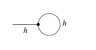
Figure 1: Diagram contributing to the Higgs 1-point function.

3.2 2-point functions

Consider mass and wave function renormalization for the pion and $h$ fields. Because of chiral symmetry no pion mass will be induced by loop corrections at any order, unlike for the $h$ field, whose mass is not protected by that symmetry. The diagrams contributing to the pion self-energy are shown in Fig. 2.

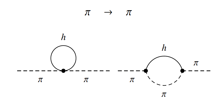
Figure 2: Diagrams contributing to the $\pi$ self-energy.

The divergent part of the amplitudes, $\Pi^{ij}_{\rm div}(p^{2})\Delta_{\varepsilon}$, and the counterterm structure are given by

$$\Pi^{ij}_{\rm div}(p^{2})= \left[p^{2}\left(a_{C}^{2}-b_{C}\right)\frac{m_{h}^{2}}{v^{2}}+p^{4}\frac{a_{C}^{2}}{v^{2}}\right]\delta_{ij}\,,$$ (3.2)

$$\Pi^{ij}_{ctr}(p^{2})= \left[p^{2}\delta_{\pi}-p^{4}\frac{4}{v^{2}}\left(\delta c_{9}-\frac{\delta v^{2}}{v^{2}}\right)\right]\delta_{ij}\,.$$ (3.3)

In an off-shell renormalization scheme, it is necessary to match all the momenta structure of the divergent amplitude with that of the counterterms, which leads to the following determination

$$\delta_{\pi}= -\left(a_{C}^{2}-b_{C}\right)\frac{m_{h}^{2}}{v^{2}}\Delta_{\varepsilon}\,,$$ (3.4)

$$\delta c_{9}-\frac{\delta v^{2}}{v^{2}}= \frac{a_{C}^{2}}{4}\Delta_{\varepsilon}\,.$$

It follows that the $\pi$ wave function renormalization has no divergent part whenever $a_{C}^{2}=b_{C}$, which happens for instance in the case of the SM ($a_{C}=b_{C}=1$). Note as well that the absence of a constant term in eq. (3.2) translates into massless pions at 1-loop level, as mandated by chiral symmetry at any loop order. Furthermore, the $p^{4}$ term stems from the $h-\pi$ coupling $a_{C}$, which is an entire new feature compared to the nonlinear $\sigma$ model renormalization. This term demands the presence of a $\Box\bm{\pi}\Box\bm{\pi}$ counterterm in the $\mathcal{L}_{4}$ Lagrangian, as expected by naive dimensional analysis.

Turning to the Higgs particle, the diagrams contributing to its self-energy are shown in Fig. 3, with the divergent part and the required counterterm structure given by

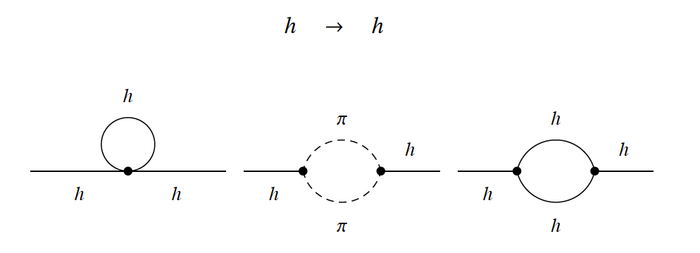
Figure 3: Diagrams contributing to the Higgs self-energy.

$$\Pi_{\rm div}(p^{2})= p^{4}\frac{\left(3a_{C}^{2}+a_{H}^{2}\right)}{2v^{2}}+p^{2}\left(-\frac{\mu_{3}}{v}a_{H}+\frac{m_{h}^{2}\left(5a_{H}^{2}-b_{H}\right)}{v^{2}}\right)$$

$$+ \left(\frac{1}{2}\mu_{3}^{2}+\frac{1}{2}m_{h}^{2}\left(\lambda-8\frac{\mu_{3}}{v}a_{H}\right)+\frac{m_{h}^{4}\left(6a_{H}^{2}-b_{H}\right)}{v^{2}}\right),$$ (3.5)

$$\Pi_{ctr}(p^{2})= p^{4}\frac{2\delta c_{\Box H}}{v^{2}}+p^{2}\delta_{h}-\delta m_{h}^{2}\,.$$ (3.6)

It follows that the required counterterms are given by

$$\delta_{h}= \left[\frac{\mu_{3}}{v}a_{H}+\frac{m_{h}^{2}\left(b_{H}-5a_{H}^{2}\right)}{v^{2}}\right]\Delta_{\varepsilon},$$ (3.7)

$$\delta m_{h}^{2}= \left[\frac{1}{2}\mu_{3}^{2}+\frac{1}{2}m_{h}^{2}\left(\lambda-8\frac{\mu_{3}}{v}a_{H}\right)+\frac{m_{h}^{4}\left(6a_{H}^{2}-b_{H}\right)}{v^{2}}\right]\Delta_{\varepsilon},$$

$$\delta c_{\Box H}= -\frac{1}{4}\left(3a_{C}^{2}+a_{H}^{2}\right)\Delta_{\varepsilon}.$$

This result implies that a non-vanishing $a_{C}$ (as in the SM limit) and/or $a_{H}$ leads to a $p^{4}$ term in the counterterm Lagrangian, requiring a $\Box h\Box h$ term in $\mathcal{L}_{4}$. In this scheme, a Higgs wave function renormalization is operative only in deviations from the SM with non-vanishing $a_{H}$ and/or $b_{H}$.

3.3 3-point functions

The calculational details for the 3- and 4-point functions will not be explicitly shown as they are not particularly illuminating . Vertices with an odd number of legs necessarily involve at least one Higgs particle.

$hhh$

Let us consider first the $hhh$ amplitude at one loop. The relevant diagrams to be computed are displayed in Fig. 4.

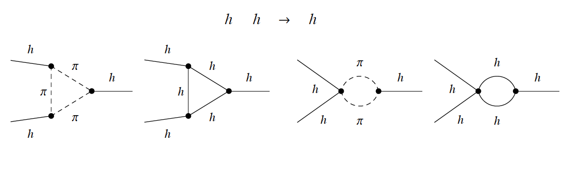
Figure 4: Diagrams contributing to the $hh\rightarrow h$ amplitude, not including diagrams obtained by crossing.

As $h$ behaves as a generic singlet, the vertices involving uniquely external $h$ legs which appear in the Lagrangian Eq. (2.1) will span all possible momentum structures that can result from one-loop amplitudes. Hence any divergence emerging on amplitudes involving only external $h$ particles will be easily absorbable. The specific results for the counterterms emerging from $\mathcal{L}_{0}$ and $\mathcal{L}_{2}$ can be found in Appendix A.

$\pi\pi h$

The diagrams for $\pi\pi h$ amplitudes are shown in Fig. 5. The one-loop divergences are studied in detail in Appendix A; for instance, it turns out that neither $\delta a_{C}$ nor $\delta a_{9}$ are induced in the SM limit. Chiral symmetry restricts the possible structures spanned by the pure $\pi$ and $h-\pi$ operators. Because of this, it turns out that part of the divergent amplitude induced by the last diagram in Fig. 5 cannot be cast as a function of the $\mathcal{L}_{2}$ and $\mathcal{L}_{4}$ operators, that is, it cannot be reabsorbed by chiral-invariant counterterms, and furthermore its coefficient depends on the pion parametrization used: an apparent non chiral-invariant divergence (NID) has been identified. NIDs are an artefact of the apparent breaking of chiral symmetry when the one-loop analysis is treated in perturbation theory [21] and have no physical impact as they vanish for on-shell amplitudes. While long ago NIDs had been isolated in perturbative analysis of four-pion vertices in the non-linear sigma model [19], the result obtained here is a new type of NID: a three-point function involving the Higgs particle, corresponding to the chiral non-invariant operator

$$\mathcal{O}_{1}^{\rm NID}=-a_{C}\left(\frac{3}{2}+5\eta\right)\frac{\Delta_{\varepsilon}}{v^{3}}\,\,\bm{\pi}\Box\bm{\pi}\Box h\,.\,$$ (3.8)

This coupling cannot be reabsorbed as part of a chiral invariant counterterm, but its contribution to on-shell amplitudes indeed vanishes. It is interesting to note that while the renormalization conditions of all physical parameters turn out to be independent of the choice of U parametrization, as they should, NIDs exhibit instead an explicit $\eta$ dependence, as illustrated by Eq. (3.8). This pattern will be also present in the renormalization of 4-point functions, developed next.

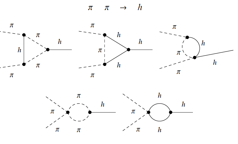
Figure 5: Diagrams contributing to the $\pi\pi\rightarrow h$ scattering amplitude, not including diagrams obtained by crossing.

3.4 4-point functions

The analysis of this set of correlation functions turns out to be tantalizing when comparing the results for mixed $\pi-h$ vertices with those for pure pionic ones .

$\pi\pi hh$

The computation of the $\pi\pi\rightarrow hh$ one-loop amplitude shows that the renormalization procedure requires the presence of all possible chiral invariant $hh\pi\pi$ counterterms in the Lagrangian, in the most general case.

Furthermore, we have identified new NIDs in $hh\pi\pi$ amplitudes:

$$\mathcal{O}^{\rm NID}_{2}=+(2a_{C}^{2}-b_{C})\left(\frac{3}{2}+5\eta\right)\frac{\Delta_{\varepsilon}}{v^{4}}\,\,\bm{\pi}\Box\bm{\pi}\,h\Box h\,,$$ (3.9)

$$\mathcal{O}^{\rm NID}_{3}=+(a_{C}^{2}-b_{C})\left(\frac{3}{2}+5\eta\right)\frac{\Delta_{\varepsilon}}{v^{4}}\,\,\bm{\pi}\Box\bm{\pi}\,\partial_{\mu}h\partial^{\mu}h\,,$$

$$\mathcal{O}^{\rm NID}_{4}=-2a_{C}^{2}\left(\frac{3}{2}+5\eta\right)\frac{\Delta_{\varepsilon}}{v^{4}}\,\,\bm{\pi}\partial_{\mu}\bm{\pi}\,\partial^{\mu}h\Box h\,.$$

While these NIDs differ from that for the three-point function in Eq. (3.8) in their counterterm structure, they all share an intriguing fact: to be proportional to the factor $(3/2+5\eta)$. Therefore a proper choice of parametrization, i.e. $\eta=-3/10$, removes all mixed $h-\pi$ NIDs. That value of $\eta$ is of no special significance as fas as we know, and in fact there is no choice of parametrization that can avoid all noninvariant divergencies, as proved next.

$\pi\mathbf{\pi}\pi\pi$

Consider now $\pi\pi\rightarrow\pi\pi$ amplitudes. Only two counterterms are necessary to reabsorb chiral-invariant divergencies, namely $\delta c_{6}$ and $\delta c_{11}$. In this case, we find no other NIDs than those already present in the nonlinear $\sigma$ model [19], which stemmed from the insertion in the loop of the four-pion vertex (whose coupling depends on $\eta$). Our analysis shows that the four-$\pi$ NIDs read:

$$\mathcal{O}_{5}^{\rm NID}=+\left(9\eta^{2}+5\eta+\frac{3}{4}\right)\frac{\Delta_{\varepsilon}}{v^{4}}\,(\bm{\pi}\Box\bm{\pi})^{2},$$ (3.10)

$$\mathcal{O}_{6}^{\rm NID}=+\left[1+4\eta+\left(\frac{1}{2}+\eta\right)a_{C}^{2}\right]\frac{\Delta_{\varepsilon}}{v^{4}}\,(\bm{\pi}\Box\bm{\pi})(\partial_{\mu}\bm{\pi}\partial^{\mu}\bm{\pi}),$$

$$\mathcal{O}_{7}^{\rm NID}=+2\eta^{2}\frac{\Delta_{\varepsilon}}{v^{4}}\,\bm{\pi}^{2}(\Box\bm{\pi})^{2},$$

$$\mathcal{O}_{8}^{\rm NID}=+2\eta\left(a_{C}^{2}-1\right)\frac{\Delta_{\varepsilon}}{v^{4}}\,(\Box\bm{\pi}\partial_{\mu}\bm{\pi})(\bm{\pi}\partial^{\mu}\bm{\pi}).$$

As expected, the parametrization freedom – the dependence on the $\eta$ parameter – appears only in NIDs, and never on chiral-invariant counterterms, as the latter describe physical processes. Furthermore, the contribution of all NIDs to on-shell amplitudes vanishes as expected . Finally, the consideration of the ensemble of three and four-point NIDs in Eqs. (3.8), (3.9) and (3.10) shows inmediately that no parametrization can remove all NIDs: it is possible to eliminate those involving $h$ , but no value of $\eta$ would remove all pure pionic ones.

$hhhh$

The renormalization procedure for $hh\rightarrow hh$ amplitudes is straightforward. It results in contributions to $\delta a_{\Delta H}$, $\delta c_{DH}$, and $\delta b_{H}$. Interestingly, Appendix B illustrates that large coefficients are present in some terms of the RGE for $b_{H}$ and $\lambda$; this might a priori translate into measurable effects when comparing data at different scales, if ever deviations from the SM predictions are detected, see Sect. (4).

There is a particularity of the off-shell renormalization scheme which deserves to be pointed out. A closer look at the counterterms reveals that, in the SM case, that is

$$a_{C}=b_{C}=1,\quad a_{H}=b_{H}=0,\quad\mu_{3}=3\frac{m_{h}^{2}}{v}\quad and\quad\lambda=3\frac{m_{h}^{2}}{v^{2}},$$ (3.11)

several BSM operator coefficients do not vanish. Although at first this might look counterintuitive, when calculating physical amplitudes the contribution of these non-vanishing operator coefficients all combine in such a way that the overall BSM contribution indeed cancels. The same pattern propagates to the renormalization group equations discussed in Sect. 4.

3.5 Dealing with the apparent non-invariant divergencies

For the nonlinear $\sigma$ model the issue of NIDs was analyzed long ago [22, 30, 31, 32, 33, 19]). In that case, it was finally proven that a nonlinear redefinition of the pion field which includes space-time derivatives could reabsorb them [19]. This method reveals a deeper rationale in understanding the issue, as Lagrangians related by a local field redefinition are equivalent, even when it involves derivatives [34, 35, 36, 37]. Consequently, if via a general pion field redefinition

$$\bm{\pi}\rightarrow\bm{\pi}\,f(\bm{\pi},h,\partial_{\mu}\bm{\pi},\partial_{\mu}h,\dots)\,,$$

with $f(0)=1$, the Lagrangian is shifted

$$\mathcal{L}\rightarrow\mathcal{L}^{\prime}=\mathcal{L}+\delta\mathcal{L}\,,$$

from the equivalence between $\mathcal{L}$ and $\mathcal{L}^{\prime}$ it follows that $\delta\mathcal{L}$ must be unphysical. Thus, if an approppriate pion field redefinition is found which is able to absorb all NDIs, it automatically implies that NDIs do not contribute to the $S$-matrix, and therefore that chiral symmetry remains unbroken. In other words, the non-invariant operators can be identifed with quantities in the functional generator that vanish upon performing the path integral.

Let us consider the following pion redefinition, in which we propose new terms not considered previously and which contain the $h$ field:

$$\pi_{i}\rightarrow \,\pi_{i}\left(1+\frac{\alpha_{1}}{2v^{4}}\bm{\pi}\Box\bm{\pi}+\frac{\alpha_{2}}{2v^{4}}\partial_{\mu}\bm{\pi}\partial^{\mu}\bm{\pi}+\frac{\beta}{2v^{3}}\Box h+\frac{\tilde{\gamma}_{1}}{2v^{4}}h\Box h+\frac{\gamma_{2}}{2v^{4}}\partial_{\mu}h\partial^{\mu}h\right)$$ (3.12)

$$\qquad+\frac{\alpha_{3}}{2v^{4}}\Box\pi_{i}(\bm{\pi}\bm{\pi})+\frac{\alpha_{4}}{2v^{4}}\partial_{\mu}\pi_{i}(\bm{\pi}\partial^{\mu}\bm{\pi}).$$

The application of this redefinition to $\mathcal{L}_{4}$ is immaterial, as it would only induce couplings of higher order. As all terms in the shift contain two derivatives, when applied to $\mathcal{L}_{2}$ contributions to $\mathcal{L}_{4}$ and NID operator coefficients do follow. Indeed, the action of Eq. (3.12) on $\mathcal{L}_{2}$ reduces to that on the term

$$\frac{1}{4}{\rm Tr}(\partial_{\mu}\textbf{U}\partial^{\mu}\textbf{U})\mathcal{F}_{C}(h)\,,$$ (3.13)

which produces the additional contribution to NDI vertices given by

$$\Delta\mathcal{L}^{\rm NID}=-\bm{\pi}\Box\bm{\pi}\left(\frac{\alpha_{1}}{v^{4}}\bm{\pi}\Box\bm{\pi}+\frac{\alpha_{2}}{v^{4}}\partial_{\mu}\bm{\pi}\partial^{\mu}\bm{\pi}+\frac{\beta}{v^{3}}\Box h+\frac{\gamma_{1}}{v^{4}}h\Box h+\frac{\gamma_{2}}{v^{4}}\partial_{\mu}h\partial^{\mu}h\right)$$

$$\qquad\quad\!-\frac{\alpha_{3}}{v^{4}}(\Box\bm{\pi}\Box\bm{\pi})(\bm{\pi}\bm{\pi})-\frac{\alpha_{4}}{v^{4}}(\Box\bm{\pi}\partial_{\mu}\bm{\pi})(\bm{\pi}\partial^{\mu}\bm{\pi})-\frac{2a_{C}\beta}{v^{4}}\bm{\pi}\partial_{\mu}\bm{\pi}\partial^{\mu}h\Box h+...$$ (3.14)

where $\gamma_{1}=2a_{C}\beta+\tilde{\gamma}_{1}$, and where the dots indicate other operators with either six derivatives or that have more than four fields and are beyond the scope of this paper. Comparing the terms in $\Delta\mathcal{L}^{\rm NID}$ with the NID operators found, Eqs. (3.8), (3.9) and (3.10), it follows that by choosing

$$\begin{aligned} &\alpha_{1}=\left(9\eta^{2}+5\eta+\frac{3}{4}\right)\Delta_{\varepsilon},\\ &\alpha_{2}=\left[1+4\eta+\left(\frac{1}{2}+\eta\right)a_{C}^{2}\right]\Delta_{\varepsilon},\\ &\alpha_{3}=2\eta^{2}\Delta_{\varepsilon},\\ &\alpha_{4}=2\eta\left(a_{C}^{2}-1\right)\Delta_{\varepsilon},\end{aligned}\qquad\begin{aligned} &\beta=-\left(\frac{3}{2}+5\eta\right)a_{C}\Delta_{\varepsilon},\\ &\gamma_{1}=\left(\frac{3}{2}+5\eta\right)\left(2a_{C}^{2}-b_{C}\right)\Delta_{\varepsilon},\\ &\gamma_{2}=\left(\frac{3}{2}+5\eta\right)\left(a_{C}^{2}-b_{C}\right)\Delta_{\varepsilon}.\\ \end{aligned}$$

all 1-loop NID are removed away.

A few comments are in order. The off-shell renormalization of one loop amplitudes is delicate and physically interesting. Because of chiral symmetry, the pure pionic or mixed pion-$h$ operators do not encode all possible momentum structures, even after pion field redefinitions. Hence, the appearance of divergent structures that can be absorbed by $\delta\mathcal{L}_{0}$, $\delta\mathcal{L}_{2}$, $\delta\mathcal{L}_{4}$ and $\Delta\mathcal{L}^{\rm NI}$ is a manisfestation of chiral invariance and of the field redefinition equivalence discussed above. We have shown consistently that NIDs appearing in the one-loop renormalization of the electroweak chiral Lagrangian do not contribute to on-shell quantities. In fact, a closer examination has revealed that the apparent chiral non-invariant divergencies emerge from loop diagrams which have at least one four-pion vertex in it, and this is why all of them depend on $\eta$. We have also shown that the presence of a light Higgs boson modifies the coefficients of the unphysical counterterms made out purely of pions, but not their structure, neither -of course- breaks chiral symmetry.

4 Renormalization Group Equations

It is straightforward to derive the RGE from the $\delta c_{i}$ divergent contributions determined in the previous section. The complete RGE set can be found in Appendix B. As illustration, the evolution of those Lagrangian coefficients which do not vanish in the SM limit is given by:

$$16\pi^{2}\frac{d}{d\ln\mu}a_{C} =\frac{1}{2}a_{C}\left[a_{H}\frac{\mu_{3}}{v}+\left(3b_{C}-5a_{H}^{2}+b_{H}\right)\frac{m_{h}^{2}}{v^{2}}\right]+a_{C}^{2}\left(\frac{\mu_{3}}{2v}-2a_{H}\frac{m_{h}^{2}}{v^{2}}\right)-\frac{3}{2}a_{C}^{3}\frac{m_{h}^{2}}{v^{2}}$$

$$-\frac{1}{2v}b_{C}\mu_{3}+2a_{H}b_{C}\frac{m_{h}^{2}}{v^{2}}\,,$$ (4.1)

$$16\pi^{2}\frac{d}{d\ln\mu}b_{C} =b_{C}\left[2a_{C}\frac{\mu_{3}}{v}+5a_{H}\frac{\mu_{3}}{v}-\frac{\lambda}{2}-\left(5a_{C}^{2}+8a_{H}a_{C}+17a_{H}^{2}-3b_{H}\right)\frac{m_{h}^{2}}{v^{2}}\right]+b_{C}^{2}\frac{m_{h}^{2}}{v^{2}}$$

$$+\frac{1}{2}\left(-4a_{C}\frac{\mu_{3}}{v}-8a_{H}\frac{\mu_{3}}{v}+\lambda\right)a_{C}^{2}+2\left(2a_{C}^{2}+4a_{H}a_{C}+6a_{H}^{2}-b_{H}\right)a_{C}^{2}\frac{m_{h}^{2}}{v^{2}}$$

$$16\pi^{2}\frac{d}{d\ln\mu}m_{h}^{2} =-\frac{1}{2}\mu_{3}^{2}+\left(5a_{H}\frac{\mu_{3}}{v}-\frac{\lambda}{2}\right)m_{h}^{2}+\left(2b_{H}-11a_{H}^{2}\right)\frac{m_{h}^{4}}{v^{2}}\,,$$ (4.2)

$$16\pi^{2}\frac{d}{d\ln\mu}\mu_{3} =\frac{1}{2}\mu_{3}\left[\left(-a_{C}^{2}+b_{C}-87a_{H}^{2}+15b_{H}\right)\frac{m_{h}^{2}}{v^{2}}-3\lambda\right]+\frac{15}{2v}\mu_{3}^{2}a_{H}$$

$$+6a_{H}\lambda\frac{m_{h}^{2}}{v}+6\left(8a_{H}^{3}-3a_{H}b_{H}\right)\frac{m_{h}^{4}}{v^{3}}\,,$$ (4.3)

$$16\pi^{2}\frac{d}{d\ln\mu}\lambda =\lambda\left[26a_{H}\frac{\mu_{3}}{v}+\left(14b_{H}-82a_{H}^{2}\right)\frac{m_{h}^{2}}{v^{2}}\right]-\frac{3}{2}\lambda^{2}+12\left(b_{H}-6a_{H}^{2}\right)\frac{\mu_{3}^{2}}{v^{2}}$$ (4.4)

$$+48a_{H}\left(8a_{H}^{2}-3b_{H}\right)\mu_{3}\frac{m_{h}^{2}}{v^{3}}-6\left(80a_{H}^{4}-48b_{H}a_{H}^{2}+3b_{H}^{2}\right)\frac{m_{h}^{4}}{v^{4}}\,.$$ (4.5)

These and the rest of the RGE in Appendix B show as well that the running of the parameters $a_{C}$, $b_{C}$, $a_{H}$, $b_{H}$, and $v^{2}$ is only induced by the couplings entering the Higgs potential, Eq. (2.5).

Note that in the RGE for the Higgs quartic self-coupling $\lambda$, Eq. (4.5), some terms are weighted by numerical factors of ${\cal O}(100)$. This suggests that if a BSM theory results in small couplings for $a_{H}$ and $b_{H}$, those terms could still induce measurable phenomenological consequences. Nevertheless, physical amplitudes will depend on a large combination of parameters, which might yield cancellations or enhancements as pointed out earlier, and only a more thorough study can lead to firm conclusions. Such large coefficients turn out to be also present in the evolution of some BSM couplings, such as the four-Higgs coupling $b_{H}$ for which

$$16\pi^{2}\frac{d}{d\ln\mu}b_{H} =b_{H}\left[20a_{H}\frac{\mu_{3}}{v}-\frac{3}{2}\lambda+\left(-a_{C}^{2}+b_{C}-87a_{H}^{2}\right)\frac{m_{h}^{2}}{v^{2}}\right]$$

$$-42\frac{\mu_{3}}{v}a_{H}^{3}+\frac{13}{2}\lambda a_{H}^{2}+\left(7b_{H}^{2}+120a_{H}^{4}\right)\frac{m_{h}^{2}}{v^{2}}\,.$$ (4.6)

On general grounds $a_{H}$ is expected to be small, and for instance the $a_{H}^{4}$ dependence in Eq. (4) is not expected to be relevant in spite of the numerical prefactor. On the other side, present data set basically no bound on the couplings involving three or more external Higgs particles, and thus the future putative impact of this evolution should not be dismissed yet.

5 Comparison with the literature

Previous works on the one-loop renormalization of the scalar sector of the non-linear Lagrangian with a light Higgs have used either the square root parametrization ($\eta=0$ in our parametrization) or the exponential one ($\eta=-1/6$), producing very interesting results, and have

• concentrated on on-shell analyses,

• disregarded the impact of $\mathcal{F}_{H}(h)$,

• disregarded fermionic operators; in practice this means to neglect all fermion masses.

This last point is not uncorrelated with the fact that the basis of independent four-derivative operators determined here has a larger number of elements than previous works about the scalar sector. Those extra bosonic operators have been shown here to be required by the counterterm procedure. It is possible to demonstrate, though, that they can be traded via EOM by other type of operators including gauge corrections and Yukawa-like operators. In a complete basis of all possible operators it is up to the practitioner to decide which set is kept, as long as it is complete and independent. When restricting instead to a given subsector, the complete and consistent treatment requires to consider all independent operators of the kind selected (anyway the renormalization procedure will indicate their need), or to state explicitly any extra assumptions to eliminate them. Some further specific comments:

Ref. [14] considers, under the first two itemized conditions above plus disregarding the impact of $V(h)$ (and in particular neglecting the Higgs mass), the scattering processes $hh\rightarrow hh$, $\pi\pi\rightarrow hh$ and $\pi\pi\rightarrow\pi\pi$. With the off-shell treatment, five additional operators result in this case with respect to those obtained in that reference (assuming the rest of their assumptions), $\mathcal{P}_{7}$, $\mathcal{P}_{9}$, $\mathcal{P}_{10}$, $\mathcal{P}_{\Box H}$ and $\mathcal{P}_{\Delta H}$ in Table 1. Note that all these operators contain either $\Box h$ or $\Box\pi$ inside; they may thus be implicitly traded by fermionic operators via EOM, and can only be disregarded if all fermion masses are neglected. Assuming this extra condition, we could reproduce their results using the EOMs. For instance, the RGEs derived here for $c_{6}$, $c_{8}$, $c_{20}$, $a_{C}$ and $b_{C}$ differ from the corresponding ones in that reference: an off-shell renormalization analysis entails the larger number of operators mentioned. In any case, we stress again that the results of both approaches coincide when calculating physical amplitudes. Another contrast appears in the running of $a_{C}$, $b_{C}$, $a_{H}$, $b_{H}$, as well as the mass, the triple, and the quartic coupling of the Higgs, for which the running is induced by the Higgs potential parameters, disregarded in that reference.

In Ref. [15] the on-shell scattering process of the longitudinal modes of the process $W^{+}W^{-}\rightarrow ZZ$ is considered, disregarding $\mathcal{F}_{H}(h)$ but including the impact of $V(h)$. Our off-shell treatment results in this case in one additional operator (assuming the rest of their assumptions) with respect to those in that reference, $\mathcal{P}_{9}$, as only processes involving four goldstone bosons were considered there. Again this extra operator contains $\Box\pi$ in all its terms and it could be neglected in practice if disregarding all fermion masses. With this extra assumption, our results reduce to theirs in the limit indicated.

6 Conclusions

We have considered the one-loop off-shell renormalization of the effective non-linear Lagrangian in the presence of a light (Higgs) scalar particle, up to four-derivative terms and taking into account the finite Higgs mass. We have concentrated in its scalar sector: goldstone bosons (that is, the longitudinal components of the SM gauge bosons) and the light scalar $h$.

Analyzing the custodial-preserving sector, we have determined the four-derivative counterterms required by the one-loop renormalization procedure, by considering the full set of 1-, 2-, 3- and 4-point functions involving pions and/or $h$. The off-shell treatment has allowed to determine all required counterterms, confirming for the sector analyzed that the generic low-energy effective non-linear Lagrangian with a light Higgs particle developed in Refs. [10, 11] is complete: all four-derivative operators of that basis and nothing else is induced by the renormalization. Those operators are linearly independent and form thus a complete basis when that sector is taken by itself. It is shown that a larger number of operators than previously considered are then needed.

As a useful analysis tool, we have also proposed here a general parametrization for the goldstone boson matrix, which at the order considered here depends on only one parameter $\eta$, and reduces to the popular parametrizations (square root, exponential etc.) for different values of $\eta$. All counterterms induced by the renormalization procedure are then easily seen to be parametrization independent, as it befits physical couplings.

Furthermore, new chiral non-invariant counterterms involving the Higgs particle and pions have been found in our perturbative analysis. These findings extend to the realm of the Higgs particle the apparent non chiral-invariant divergences identified decades ago for the non-linear sigma model [19]. Those apparent violations of chiral symmetry are an artefact of perturbative approaches, they vanish on-shell, and their origin had been tracked down to the insertion of the four-pion vertex in loops. In this paper, new non-invariant divergences are shown to appear in triple $h\pi\pi$ counterterms and in $hh\pi\pi$ ones, and shown to have the same origin. Interestingly: i) all apparently non-invariant divergences depend explicitly on $\eta$, consistent with their non-physical nature; ii) there is a value of the $\eta$ parameter for which the non-invariant divergences involving the Higgs vanish, though, while no $\eta$ value can cancel the ensemble of non-invariant divergences and in particular the pure pion ones.

Moreover, we have determined a local pion-field redefinition which includes space-time derivatives and reabsorbs automatically all apparently chiral non-invariant counterterms. This field redefinition leaves invariant the S-matrix and thus the result shows automatically that chiral symmetry remains unbroken.

For the physical counterterms induced, we observe a complete agreement with the naive dimensional analysis [17, 18] in the $h-\pi$ sector of the chiral Lagrangian. Finally, the RGEs for the scalar sector of the general non-linear effective Lagrangian for a Higgs particle have been also derived in this work. The complete set of equations can be found in Appendix B. Factors of ${\cal O}(100)$ appear accompanying certain operator coefficients in the RGEs, and those terms may thus be specially relevant when comparing future Higgs and gauge boson data obtained at different energies. On more general grounds, although present data are completely consistent with the SM predictions, going for precision in constraining small parameters may be the best way to tackle BSM physics and we should not be deterred by the task: the dream of today may be the discovery of tomorrow and the background of the future.

Appendix A The counterterms

Details about the computation of the counterterms and the renormalization of the chiral Lagrangian are given in this Appendix, including the derivation of the RGEs.

The bare parameters (denoted by $b$) written in terms of the renormalized ones and the counterterms for the $\mathcal{L}_{2}$ and $\mathcal{L}_{4}$ Lagrangians are given by

$$\begin{aligned} &h_{b}=\sqrt{Z_{h}}h,\qquad\delta_{h}\equiv Z_{h}-1,\\ &\bm{\pi}_{b}=\sqrt{Z_{\pi}}\bm{\pi},\qquad\delta_{\pi}\equiv Z_{\pi}-1,\\ \\ &v^{2}_{b}=Z_{\pi}(v^{2}+\delta v^{2})\mu^{-\varepsilon},\\ &(m_{h}^{2})^{b}=\frac{1}{Z_{h}}(m_{h}^{2}+\delta m_{h}^{2}),\\ &(\mu_{1}^{3})^{b}=\frac{1}{Z_{h}^{1/2}}\left(\mu_{1}^{3}+\delta\mu_{1}^{3}\right)\mu^{3\varepsilon/2},\\ &\mu_{3}^{b}=\frac{1}{Z_{h}^{3/2}}\left(\mu_{3}+\delta\mu_{3}\right)\mu^{\varepsilon/2},\\ &\lambda^{b}=\frac{1}{Z_{h}^{2}}\left(\lambda+\delta\lambda\right)\mu^{\varepsilon},\end{aligned}\quad\,\,\begin{aligned} \\ \\ &a_{C}^{b}=\frac{1}{Z_{\pi}^{1/2}Z_{h}^{1/2}}\left(a_{C}+\delta a_{C}+\frac{a_{C}}{2}\frac{\delta v^{2}}{v^{2}}\right),\\ &b_{C}^{b}=\frac{1}{Z_{h}}\left(b_{C}+\delta b_{C}+b_{C}\frac{\delta v^{2}}{v^{2}}\right),\\ &a_{H}^{b}=\frac{Z_{\pi}^{1/2}}{Z_{h}^{3/2}}\left(a_{H}+\delta a_{H}+\frac{a_{H}}{2}\frac{\delta v^{2}}{v^{2}}\right),\\ &b_{H}^{b}=\frac{Z_{\pi}}{Z_{h}^{2}}\left(b_{H}+\delta b_{H}+b_{H}\frac{\delta v^{2}}{v^{2}}\right),\end{aligned}$$ (A.1)

where

$$X_{i}^{b}=\left(X_{i}+\delta X_{i}+2X_{i}\frac{\delta v^{2}}{v^{2}}\right)\mu^{-\varepsilon}, X_{i}=c_{6},c_{9},c_{11},$$ (A.2)

$$X_{i}^{b}=\frac{Z_{\pi}^{1/2}}{Z_{h}^{1/2}}\left(X_{i}+\delta X_{i}+\frac{3}{2}X_{i}\frac{\delta v^{2}}{v^{2}}\right)\mu^{-\varepsilon}, X_{i}=c_{7},a_{9},c_{10},$$

$$X_{i}^{b}=\frac{Z_{\pi}}{Z_{h}}\left(X_{i}+\delta X_{i}+2X_{i}\frac{\delta v^{2}}{v^{2}}\right)\mu^{-\varepsilon}, X_{i}=a_{7},c_{8},b_{9},a_{10},c_{20},$$

$$X_{i}^{b}=\frac{Z_{\pi}}{Z_{h}}\left(X_{i}+\delta X_{i}+X_{i}\frac{\delta v^{2}}{v^{2}}\right)\mu^{-\varepsilon}, X_{i}=c_{\Box H},$$

$$X_{i}^{b}=\frac{Z_{\pi}^{3/2}}{Z_{h}^{3/2}}\left(X_{i}+\delta X_{i}+\frac{3}{2}X_{i}\frac{\delta v^{2}}{v^{2}}\right)\mu^{-\varepsilon}, X_{i}=a_{\Box H},c_{\Delta H},$$

$$X_{i}^{b}=\frac{Z_{\pi}^{2}}{Z_{h}^{2}}\left(X_{i}+\delta X_{i}+2X_{i}\frac{\delta v^{2}}{v^{2}}\right)\mu^{-\varepsilon}, X_{i}=b_{\Box H},a_{\Delta H},c_{DH}.$$

The counterterms required to absorb the divergencies of the $hhh$ 3-point function are

$$\delta a_{\Box H}=\frac{1}{2}\left(-\frac{3a_{C}b_{C}}{2}-\frac{a_{H}b_{H}}{2}+3a_{C}^{3}+a_{H}^{3}\right)\Delta_{\varepsilon},$$ (A.3)

$$\delta c_{\Delta H}=\frac{1}{2}\left(-3a_{C}b_{C}+3a_{C}^{3}-a_{H}^{3}\right)\Delta_{\varepsilon},$$

$$\delta a_{H}=\left[\frac{1}{2}\left(-9\frac{\mu_{3}}{v}a_{H}^{2}+\lambda a_{H}+2\frac{\mu_{3}}{v}b_{H}\right)+a_{H}\left(15a_{H}^{2}-7b_{H}\right)\frac{m_{h}^{2}}{v^{2}}\right]\Delta_{\varepsilon},$$

$$\delta\mu_{3}=\bigg{[}\frac{3}{2}\mu_{3}\left(\lambda-4\frac{\mu_{3}}{v}a_{H}\right)+6\left(6\mu_{3}a_{H}^{2}-\lambda va_{H}-\mu_{3}b_{H}\right)\frac{m_{h}^{2}}{v^{2}}$$

$$\hskip 187.78836pt+6a_{H}\left(3b_{H}-8a_{H}^{2}\right)\frac{m_{h}^{4}}{v^{3}}\bigg{]}\Delta_{\varepsilon},$$

while those for $\pi\pi\rightarrow h$ read

$$\delta a_{C}=\frac{1}{2}\left(a_{C}^{2}-b_{C}\right)\left[2(a_{C}+2a_{H})\frac{m_{h}^{2}}{v^{2}}-\frac{\mu_{3}}{v}\right]\Delta_{\varepsilon},$$ (A.4)

$$\delta c_{7}=\frac{1}{4}\left(-a_{H}b_{C}+a_{C}^{2}a_{H}-a_{C}^{3}-2a_{C}\right)\Delta_{\varepsilon},$$

$$\delta a_{9}=-\frac{1}{8}a_{C}\left(a_{C}a_{H}+a_{C}^{2}-b_{C}\right)\Delta_{\varepsilon},$$

$$\delta c_{10}=\frac{1}{2}a_{C}\left(-a_{C}a_{H}+a_{C}^{2}+b_{C}\right)\Delta_{\varepsilon}.$$

In the case of the $\pi\pi\rightarrow hh$ amplitudes, the relevant diagrams are displayed in Fig. 6, and

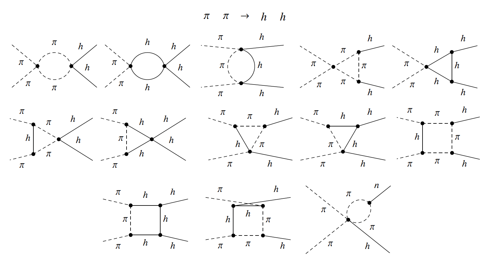
Figure 6: Diagrams contributing to the $\pi\pi\rightarrow hh$ amplitude, not including diagrams obtained by crossing.

the counterterms correspond to

$$\delta b_{C}=\frac{1}{2}\left(a_{C}^{2}-b_{C}\right)\Big{[}\left(4a_{C}+8a_{H}\right)\frac{\mu_{3}}{v}-\lambda$$ (A.5)

$$\hskip 113.81102pt-2\left(8a_{C}a_{H}+4a_{C}^{2}+12a_{H}^{2}-b_{C}-2b_{H}\right)\frac{m_{h}^{2}}{v^{2}}\Big{]}\Delta_{\varepsilon},$$

$$\delta a_{7}=\frac{1}{8}\Big{[}a_{C}^{2}\left(-4a_{H}^{2}-3b_{C}+b_{H}+4\right)+2a_{C}a_{H}b_{C}+b_{C}\left(4a_{H}^{2}-b_{H}-2\right)+4a_{C}^{4}\Big{]}\Delta_{\varepsilon}\,,$$

$$\delta c_{8}=\frac{1}{3}\left[a_{C}^{2}\left(a_{H}^{2}+b_{C}\right)-2a_{C}a_{H}b_{C}-a_{C}^{3}a_{H}+a_{C}^{4}+b_{C}^{2}\right]\Delta_{\varepsilon}\,,$$

$$\delta b_{9}=\frac{1}{4}\left[-a_{C}^{2}\left(-4a_{H}^{2}+5b_{C}+b_{H}\right)-4a_{C}a_{H}b_{C}+4a_{C}^{3}a_{H}+4a_{C}^{4}+b_{C}^{2}\right]\Delta_{\varepsilon}\,,$$

$$\delta a_{10}=\frac{1}{4}\left[a_{C}^{2}\left(4a_{H}^{2}+b_{C}-b_{H}\right)-4a_{C}a_{H}b_{C}-4a_{C}^{4}+b_{C}^{2}\right]\Delta_{\varepsilon}\,,$$

$$\delta c_{20}=\frac{1}{12}\Big{[}a_{C}^{2}\left(2a_{H}^{2}-b_{C}+6\right)+2a_{C}a_{H}b_{C}$$

$$\hskip 142.26378pt-b_{C}\left(3a_{H}^{2}+b_{C}+6\right)-2a_{C}^{3}a_{H}+2a_{C}^{4}\Big{]}\Delta_{\varepsilon}\,.$$

For $\pi\pi\rightarrow\pi\pi$ amplitudes, the relevant diagrams are displayed in Fig. 7, and

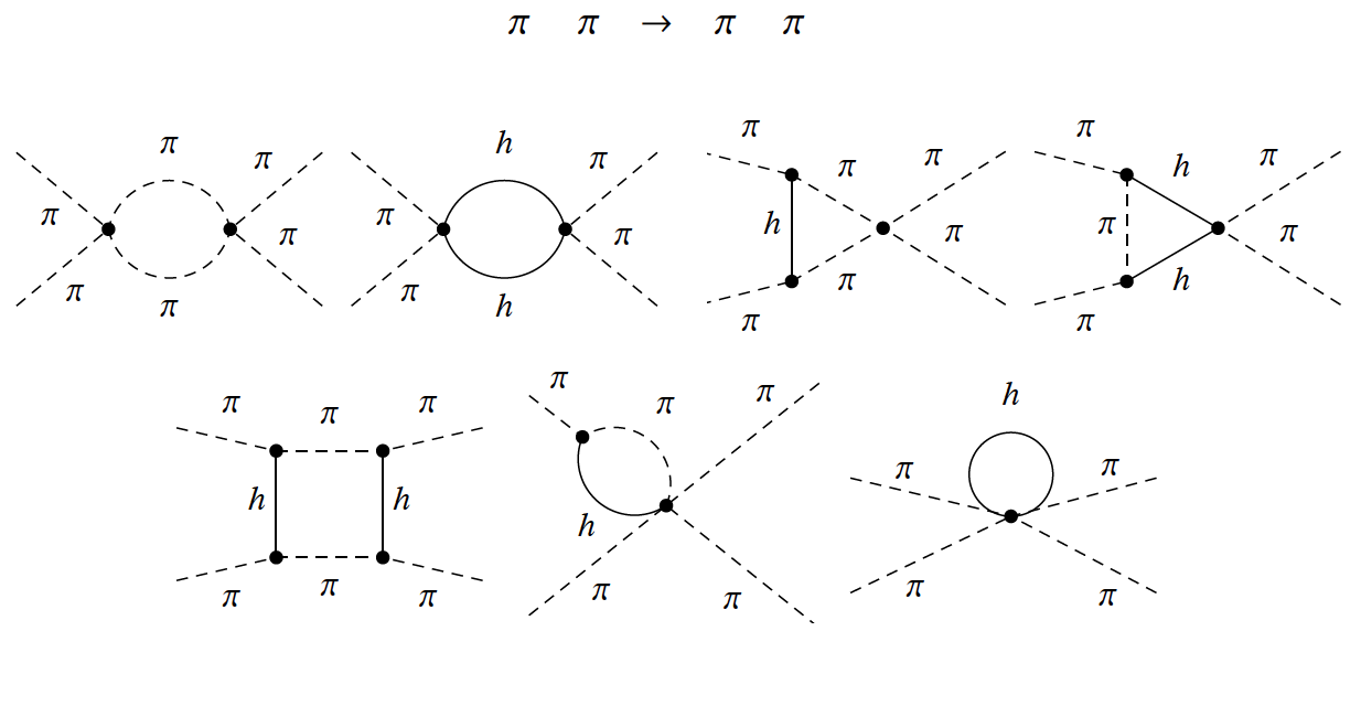
Figure 7: Diagrams contributing to the $\pi\pi\rightarrow\pi\pi$ amplitude, not including diagrams obtained by crossing.

the required counterterms are given by

$$\delta c_{6}=\frac{1}{48}\left[a_{C}^{2}\left(6b_{C}-8\right)-2a_{C}^{4}-3b_{C}^{2}-2\right]\Delta_{\varepsilon},$$ (A.6)

$$\delta c_{11}=-\frac{1}{12}\left(a_{C}^{2}-1\right)^{2}\Delta_{\varepsilon}.$$

Finally, the relevant diagrams for $hh\rightarrow hh$ amplitudes are shown in Fig. 8, and

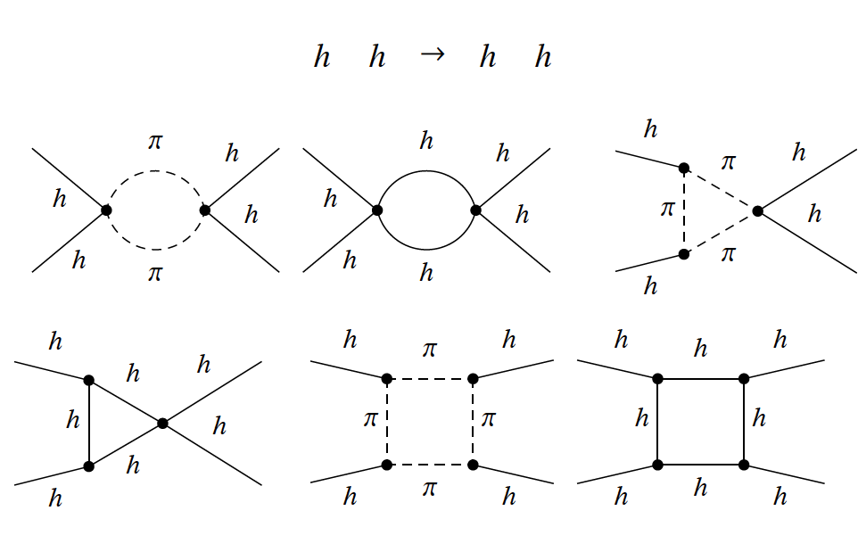
Figure 8: Diagrams contributing to the $hh\rightarrow hh$ amplitude, not including diagrams obtained by crossing.

the renormalization conditions read

$$\delta b_{H}=\Big{[}\frac{1}{2}\left(\frac{\mu_{3}}{v}\left(-40a_{H}b_{H}+84a_{H}^{3}\right)-13\lambda a_{H}^{2}+3\lambda b_{H}\right)$$ (A.7)

$$\hskip 122.34692pt+\left(87a_{H}^{2}b_{H}-120a_{H}^{4}-7b_{H}^{2}\right)\frac{m_{h}^{2}}{v^{2}}\Big{]}\Delta_{\varepsilon},$$

$$\delta b_{\Box H}=\frac{1}{4}\left[-3\left(4a_{H}^{4}+b_{C}^{2}\right)+30a_{C}^{2}b_{C}+10a_{H}^{2}b_{H}-36a_{C}^{4}-b_{H}^{2}\right]\Delta_{\varepsilon},$$

$$\delta a_{\Delta H}=-\frac{3}{4}\left(-7a_{C}^{2}b_{C}+a_{H}^{2}b_{H}+6a_{C}^{4}-2a_{H}^{4}+b_{C}^{2}\right)\Delta_{\varepsilon},$$

$$\delta c_{DH}=\Big{[}-\frac{3}{4}\left(a_{C}^{2}-b_{C}\right){}^{2}-\frac{a_{H}^{4}}{4}\Big{]}\Delta_{\varepsilon},$$

$$\delta\lambda=\Big{\{}\frac{3}{2v^{2}}\left[8\mu_{3}^{2}\left(6a_{H}^{2}-b_{H}\right)-16\lambda\mu_{3}{v}a_{H}+\lambda^{2}v^{2}\right]$$

$$\hskip 85.35826pt-12\left(-12\mu_{3}a_{H}b_{H}+32\mu_{3}a_{H}^{3}-6\lambda va_{H}^{2}+\lambda vb_{H}\right)\frac{m_{h}^{2}}{v^{3}}$$

$$\hskip 85.35826pt+6\left(-48a_{H}^{2}b_{H}+80a_{H}^{4}+3b_{H}^{2}\right)\frac{m_{h}^{4}}{v^{4}}\Big{\}}\Delta_{\varepsilon}.$$

Appendix B The Renormalization Group Equations

This Appendix provides the expressions for the RGE of all couplings discussed above, at the order considered in this paper:

$$16\pi^{2}\frac{d}{d\ln\mu}a_{C} =a_{C}\left[\left(5a_{H}^{2}-3b_{C}-b_{H}\right)\frac{m_{h}^{2}}{v^{2}}-a_{H}\frac{\mu_{3}}{v}\right]$$

$$+a_{C}^{2}\left(4a_{H}\frac{m_{h}^{2}}{v^{2}}-\frac{\mu_{3}}{v}\right)+3a_{C}^{3}\frac{m_{h}^{2}}{v^{2}}+b_{C}\frac{\mu_{3}}{v}-4a_{H}b_{C}\frac{m_{h}^{2}}{v^{2}}\,\,,$$ (B.1)

$$16\pi^{2}\frac{d}{d\ln\mu}b_{C} =b_{C}\left[2\left(5a_{C}^{2}+8a_{C}a_{H}+17a_{H}^{2}-3b_{H}\right)\frac{m_{h}^{2}}{v^{2}}+\lambda-2(2a_{C}+5a_{H})\frac{\mu_{3}}{v}\right]$$

$$-2b_{C}^{2}\frac{m_{h}^{2}}{v^{2}}+a_{C}^{2}\left(-\lambda+4a_{C}\frac{\mu_{3}}{v}+8a_{H}\frac{\mu_{3}}{v}\right)$$

$$-4a_{C}^{2}\left(2a_{C}^{2}+4a_{C}a_{H}+6a_{H}^{2}-b_{H}\right)\frac{m_{h}^{2}}{v^{2}}\,\,,$$ (B.2)

$$16\pi^{2}\frac{d}{d\ln\mu}a_{H} =a_{H}\left[\lambda-\left(a_{C}^{2}-b_{C}+17b_{H}\right)\frac{m_{h}^{2}}{v^{2}}\right]-12a_{H}^{2}\frac{\mu_{3}}{v}+45a_{H}^{3}\frac{m_{h}^{2}}{v^{2}}+2b_{H}\frac{\mu_{3}}{v}\,\,,$$ (B.3)

$$16\pi^{2}\frac{d}{d\ln\mu}b_{H} =b_{H}\left[2\left(-a_{C}^{2}+97a_{H}^{2}+b_{C}\right)\frac{m_{h}^{2}}{v^{2}}-44a_{H}\frac{\mu_{3}}{v}+3\lambda\right]-18b_{H}^{2}\frac{m_{h}^{2}}{v^{2}}$$

$$+a_{H}^{2}\left(-13\lambda+84a_{H}\frac{\mu_{3}}{v}\right)-240a_{H}^{4}\frac{m_{h}^{2}}{v^{2}}\,\,,$$ (B.4)

$$16\pi^{2}\frac{d}{d\ln\mu}m_{h}^{2} =m_{h}^{2}\left(\lambda-10a_{H}\frac{\mu_{3}}{v}\right)+\left(22a_{H}^{2}-4b_{H}\right)\frac{m_{h}^{4}}{v^{2}}+\mu_{3}^{2}\,\,,$$ (B.5)

$$16\pi^{2}\frac{d}{d\ln\mu}\mu_{3} =\mu_{3}\left[\left(87a_{H}^{2}-15b_{H}\right)\frac{m_{h}^{2}}{v^{2}}+3\lambda\right]-15a_{H}\frac{\mu_{3}^{2}}{v}$$

$$-12\lambda a_{H}\frac{m_{h}^{2}}{v}-\left(96a_{H}^{3}-36a_{H}b_{H}\right)\frac{m_{h}^{4}}{v^{3}}\,\,,$$ (B.6)

$$16\pi^{2}\frac{d}{d\ln\mu}\lambda =\lambda\left[4\left(41a_{H}^{2}-7b_{H}\right)\frac{m_{h}^{2}}{v^{2}}-52a_{H}\frac{\mu_{3}}{v}\right]+3\lambda^{2}+24\left(6a_{H}^{2}-b_{H}\right)\frac{\mu_{3}^{2}}{v^{2}}$$

$$-96a_{H}\left(8a_{H}^{2}-3b_{H}\right)\frac{\mu_{3}m_{h}^{2}}{v^{3}}+12\left(80a_{H}^{4}-48a_{H}^{2}b_{H}+3b_{H}^{2}\right)\frac{m_{h}^{4}}{v^{4}}\,\,,$$ (B.7)

$$16\pi^{2}\frac{d}{d\ln\mu}v^{2} =-2\left(a_{C}^{2}-b_{C}\right)m_{h}^{2}\,\,,$$ (B.8)

$$16\pi^{2}\frac{d}{d\ln\mu}c_{6} =-\frac{1}{24}\left[2+2a_{C}^{4}+3b_{C}^{2}-a_{C}^{2}\left(-8+6b_{C}\right)\right]\,\,,$$ (B.9)

$$16\pi^{2}\frac{d}{d\ln\mu}c_{7} =-c_{7}\left[\left(a_{C}^{2}-5a_{H}^{2}-b_{C}+b_{H}\right)\frac{m_{h}^{2}}{v^{2}}+a_{H}\frac{\mu_{3}}{v}\right]$$

$$+\frac{1}{2}\left(-2a_{C}-a_{C}^{3}+a_{C}^{2}a_{H}-a_{H}b_{C}\right)\,\,,$$ (B.10)

$$16\pi^{2}\frac{d}{d\ln\mu}a_{7} =-a_{7}\left[2\left(a_{C}^{2}-5a_{H}^{2}-b_{C}+b_{H}\right)\frac{m_{h}^{2}}{v^{2}}+2a_{H}\frac{\mu_{3}}{v}\right]$$

$$+\frac{1}{4}\left[4a_{C}^{4}+2a_{C}a_{H}b_{C}+b_{C}\left(-2+4a_{H}^{2}-b_{H}\right)+a_{C}^{2}\left(4-4a_{H}^{2}-3b_{C}+b_{H}\right)\right]\,\,,$$ (B.11)

$$16\pi^{2}\frac{d}{d\ln\mu}c_{8} =-c_{8}\left[2\left(a_{C}^{2}-5a_{H}^{2}-b_{C}+b_{H}\right)\frac{m_{h}^{2}}{v^{2}}+2a_{H}\frac{\mu_{3}}{v}\right]$$

$$+\frac{2}{3}\left[a_{C}^{4}-a_{C}^{3}a_{H}-2a_{C}a_{H}b_{C}+b_{C}^{2}+a_{C}^{2}\left(a_{H}^{2}+b_{C}\right)\right]\,\,,$$ (B.12)

$$16\pi^{2}\frac{d}{d\ln\mu}c_{9} =\frac{a_{C}^{2}}{2}\,\,,$$ (B.13)

$$16\pi^{2}\frac{d}{d\ln\mu}a_{9} =-a_{9}\left[\left(a_{C}^{2}-5a_{H}^{2}-b_{C}+b_{H}\right)\frac{m_{h}^{2}}{v^{2}}+a_{H}\frac{\mu_{3}}{v}\right]$$

$$-\frac{1}{2}a_{C}\left(a_{C}^{2}+a_{C}a_{H}-b_{C}\right)\,\,,$$ (B.14)

$$16\pi^{2}\frac{d}{d\ln\mu}b_{9} =-b_{9}\left[2\left(a_{C}^{2}-5a_{H}^{2}-b_{C}+b_{H}\right)\frac{m_{h}^{2}}{v^{2}}+2a_{H}\frac{\mu_{3}}{v}\right]$$

$$+\frac{1}{2}\left[4a_{C}^{4}+4a_{C}^{3}a_{H}-4a_{C}a_{H}b_{C}+b_{C}^{2}+a_{C}^{2}\left(4a_{H}^{2}-5b_{C}-b_{H}\right)\right]\,\,,$$ (B.15)

$$16\pi^{2}\frac{d}{d\ln\mu}c_{10} =-c_{10}\left[\left(a_{C}^{2}-5a_{H}^{2}-b_{C}+b_{H}\right)\frac{m_{h}^{2}}{v^{2}}+a_{H}\frac{\mu_{3}}{v}\right]+a_{C}\left(a_{C}^{2}-a_{C}a_{H}+b_{C}\right)\,\,,$$ (B.16)

$$16\pi^{2}\frac{d}{d\ln\mu}a_{10} =-a_{10}\left[2\left(a_{C}^{2}-5a_{H}^{2}-b_{C}+b_{H}\right)\frac{m_{h}^{2}}{v^{2}}+2a_{H}\frac{\mu_{3}}{v}\right]$$

$$+\frac{1}{2}\left(-4a_{C}^{4}-4a_{C}a_{H}b_{C}+b_{C}^{2}+a_{C}^{2}\left(4a_{H}^{2}+b_{C}-b_{H}\right)\right)\,\,,$$ (B.17)

$$16\pi^{2}\frac{d}{d\ln\mu}c_{11} =-\frac{1}{6}\left(a_{C}^{2}-1\right)^{2}\,\,,$$ (B.18)

$$16\pi^{2}\frac{d}{d\ln\mu}c_{20} =-c_{20}\left[2\left(a_{C}^{2}-5a_{H}^{2}-b_{C}+b_{H}\right)\frac{m_{h}^{2}}{v^{2}}+2a_{H}\frac{\mu_{3}}{v}\right]$$ (B.19)

$$+\frac{1}{6}\left[2a_{C}^{4}-2a_{C}^{3}a_{H}+a_{C}^{2}\left(6+2a_{H}^{2}-b_{C}\right)+2a_{C}a_{H}b_{C}-b_{C}\left(6+3a_{H}^{2}+b_{C}\right)\right]\,\,,$$

$$16\pi^{2}\frac{d}{d\ln\mu}c_{\Box H} =-c_{\Box H}\left[2\left(a_{C}^{2}-5a_{H}^{2}-b_{C}+b_{H}\right)\frac{m_{h}^{2}}{v^{2}}+2a_{H}\frac{\mu_{3}}{v}\right]+\frac{1}{2}\left(-3a_{C}^{2}-a_{H}^{2}\right)\,\,,$$ (B.20)

$$16\pi^{2}\frac{d}{d\ln\mu}a_{\Box H} =-a_{\Box H}\left[3\left(a_{C}^{2}-5a_{H}^{2}-b_{C}+b_{H}\right)\frac{m_{h}^{2}}{v^{2}}+3a_{H}\frac{\mu_{3}}{v}\right]$$

$$+3a_{C}^{3}+a_{H}^{3}-\frac{3a_{C}b_{C}}{2}-\frac{a_{H}b_{H}}{2}\,\,,$$ (B.21)

$$16\pi^{2}\frac{d}{d\ln\mu}b_{\Box H} =-b_{\Box H}\left[4\left(a_{C}^{2}-5a_{H}^{2}-b_{C}+b_{H}\right)\frac{m_{h}^{2}}{v^{2}}+4a_{H}\frac{\mu_{3}}{v}\right]$$

$$-18a_{C}^{4}-6a_{H}^{4}+15a_{C}^{2}b_{C}-\frac{3b_{C}^{2}}{2}+5a_{H}^{2}b_{H}-\frac{b_{H}^{2}}{2}\,\,,$$ (B.22)

$$16\pi^{2}\frac{d}{d\ln\mu}c_{\Delta H} =-c_{\Delta H}\left[3\left(a_{C}^{2}-5a_{H}^{2}-b_{C}+b_{H}\right)\frac{m_{h}^{2}}{v^{2}}+3a_{H}\frac{\mu_{3}}{v}\right]+3a_{C}^{3}-a_{H}^{3}-3a_{C}b_{C}\,\,,$$ (B.23)

$$16\pi^{2}\frac{d}{d\ln\mu}a_{\Delta H} =-a_{\Delta H}\left[4\left(a_{C}^{2}-5a_{H}^{2}-b_{C}+b_{H}\right)\frac{m_{h}^{2}}{v^{2}}+4a_{H}\frac{\mu_{3}}{v}\right]$$

$$-\frac{3}{2}\left(6a_{C}^{4}-2a_{H}^{4}-7a_{C}^{2}b_{C}+b_{C}^{2}+a_{H}^{2}b_{H}\right)\,\,,$$ (B.24)

$$16\pi^{2}\frac{d}{d\ln\mu}c_{DH} =-c_{DH}\left[4\left(a_{C}^{2}-5a_{H}^{2}-b_{C}+b_{H}\right)\frac{m_{h}^{2}}{v^{2}}+4a_{H}\frac{\mu_{3}}{v}\right]$$

$$-\frac{1}{2}\left[a_{H}^{4}+3\left(a_{C}^{2}-b_{C}\right)^{2}\right]\,\,.$$ (B.25)

References

- [1] D. B. Kaplan and H. Georgi, SU(2) x U(1) Breaking by Vacuum Misalignment, Phys.Lett. B136 (1984) 183.
- [2] H. Georgi and D. B. Kaplan, Composite Higgs and Custodial SU(2), Phys.Lett. B145 (1984) 216.
- [3] M. J. Dugan, H. Georgi, and D. B. Kaplan, Anatomy of a Composite Higgs Model, Nucl.Phys. B254 (1985) 299.
- [4] K. Agashe, R. Contino, and A. Pomarol, The Minimal composite Higgs model, Nucl.Phys. B719 (2005) 165–187, [hep-ph/0412089].
- [5] R. Contino, L. Da Rold, and A. Pomarol, Light custodians in natural composite Higgs models, Phys.Rev. D75 (2007) 055014, [hep-ph/0612048].
- [6] G. Panico, M. Redi, A. Tesi, and A. Wulzer, On the Tuning and the Mass of the Composite Higgs, arXiv:1210.7114.
- [7] B. Grinstein and M. Trott, A Higgs-Higgs bound state due to new physics at a TeV, Phys.Rev. D76 (2007) 073002, [arXiv:0704.1505].
- [8] R. Contino, C. Grojean, M. Moretti, F. Piccinini, and R. Rattazzi, Strong Double Higgs Production at the LHC, JHEP 1005 (2010) 089, [arXiv:1002.1011].
- [9] A. Azatov, R. Contino, and J. Galloway, Model-Independent Bounds on a Light Higgs, JHEP 1204 (2012) 127, [arXiv:1202.3415].
- [10] R. Alonso, M. Gavela, L. Merlo, S. Rigolin, and J. Yepes, The Effective Chiral Lagrangian for a Light Dynamical ”Higgs Particle”, Phys.Lett. B722 (2013) 330–335, [arXiv:1212.3305].
- [11] I. Brivio, T. Corbett, O. Éboli, M. Gavela, J. Gonzalez-Fraile, et. al., Disentangling a dynamical Higgs, JHEP 1403 (2014) 024, [arXiv:1311.1823].
- [12] R. Alonso, I. Brivio, G. M. B., L. Merlo, and S. Rigolin, Sigma Decomposition, arXiv:1408.XXXX.
- [13] A. C. Longhitano, Low-Energy Impact of a Heavy Higgs Boson Sector, Nucl.Phys. B188 (1981) 118.
- [14] R. L. Delgado, A. Dobado, and F. J. Llanes-Estrada, One-loop and scattering from the electroweak Chiral Lagrangian with a light Higgs-like scalar, JHEP 1402 (2014) 121, [arXiv:1311.5993].
- [15] D. Espriu, F. Mescia, and B. Yencho, Radiative corrections to WL WL scattering in composite Higgs models, Phys.Rev. D88 (2013) 055002, [arXiv:1307.2400].
- [16] R. Delgado, A. Dobado, M. Herrero, and J. Sanz-Cillero, One-loop and from the Electroweak Chiral Lagrangian with a light Higgs-like scalar, arXiv:1404.2866.
- [17] A. Manohar and H. Georgi, Chiral Quarks and the Nonrelativistic Quark Model, Nucl.Phys. B234 (1984) 189.
- [18] E. E. Jenkins, A. V. Manohar, and M. Trott, Naive Dimensional Analysis Counting of Gauge Theory Amplitudes and Anomalous Dimensions, Phys.Lett. B726 (2013) 697–702, [arXiv:1309.0819].
- [19] T. Appelquist and C. W. Bernard, The Nonlinear Model in the Loop Expansion, Phys.Rev. D23 (1981) 425.
- [20] I. Gerstein, R. Jackiw, S. Weinberg, and B. Lee, Chiral loops, Phys.Rev. D3 (1971) 2486–2492.
- [21] S. Weinberg, Nonlinear realizations of chiral symmetry, Phys.Rev. 166 (1968) 1568–1577.
- [22] J. Charap, Closed-loop calculations using a chiral-invariant lagrangian, Phys.Rev. D2 (1970) 1554–1561.
- [23] G. Giudice, C. Grojean, A. Pomarol, and R. Rattazzi, The Strongly-Interacting Light Higgs, JHEP 0706 (2007) 045, [hep-ph/0703164].
- [24] R. Mertig, M. Bohm, and A. Denner, FEYN CALC: Computer algebraic calculation of Feynman amplitudes, Comput.Phys.Commun. 64 (1991) 345–359.
- [25] A. Alloul, N. D. Christensen, C. Degrande, C. Duhr, and B. Fuks, FeynRules 2.0 - A complete toolbox for tree-level phenomenology, Comput.Phys.Commun. 185 (2014) 2250–2300, [arXiv:1310.1921].
- [26] J. Kublbeck, M. Bohm, and A. Denner, Feyn Arts: Computer Algebraic Generation of Feynman Graphs and Amplitudes, Comput.Phys.Commun. 60 (1990) 165–180.
- [27] T. Hahn, Generating Feynman diagrams and amplitudes with FeynArts 3, Comput.Phys.Commun. 140 (2001) 418–431, [hep-ph/0012260].
- [28] T. Hahn and M. Perez-Victoria, Automatized one loop calculations in four-dimensions and D-dimensions, Comput.Phys.Commun. 118 (1999) 153–165, [hep-ph/9807565].
- [29] S. Saa, Master thesis. 2014. To appear.
- [30] D. Kazakov, V. Pervushin, and S. Pushkin, Invariant Renormalization for the Field Theories with Nonlinear Symmetry, Teor.Mat.Fiz. 31 (1977) 169–176.
- [31] D. Kazakov, V. Pervushin, and S. Pushkin, An Invariant Renormalization Method for Nonlinear Realizations of the Dynamical Symmetries, Theor.Math.Phys. 31 (1977) 389.
- [32] B. de Wit and M. T. Grisaru, On-shell Counterterms and Nonlinear Invariances, Phys.Rev. D20 (1979) 2082.
- [33] J. Honerkamp, Chiral multiloops, Nucl.Phys. B36 (1972) 130–140.
- [34] M. Ostrogradsky, Mémoire sur les équations différentielles relatives an probléme des isopérimétres. 1850.
- [35] C. Grosse-Knetter, Effective Lagrangians with higher derivatives and equations of motion, Phys.Rev. D49 (1994) 6709–6719, [hep-ph/9306321].
- [36] S. Scherer and H. Fearing, Field transformations and the classical equation of motion in chiral perturbation theory, Phys.Rev. D52 (1995) 6445–6450, [hep-ph/9408298].
- [37] C. Arzt, Reduced effective Lagrangians, Phys.Lett. B342 (1995) 189–195, [hep-ph/9304230].