Is the Quantum State Real?
An Extended Review of $\psi$-ontology Theorems

Towards the end of 2011, Pusey, Barrett and Rudolph derived a theorem that aimed to show that the quantum state must be ontic (a state of reality) in a broad class of realist approaches to quantum theory. This result attracted a lot of attention and controversy. The aim of this review article is to review the background to the Pusey–Barrett–Rudolph Theorem, to provide a clear presentation of the theorem itself, and to review related work that has appeared since the publication of the Pusey–Barrett–Rudolph paper. In particular, this review: Explains what it means for the quantum state to be ontic or epistemic (a state of knowledge); Reviews arguments for and against an ontic interpretation of the quantum state as they existed prior to the Pusey–Barrett–Rudolph Theorem; Explains why proving the reality of the quantum state is a very strong constraint on realist theories in that it would imply many of the known no-go theorems, such as Bell’s Theorem and the need for an exponentially large ontic state space; Provides a comprehensive presentation of the Pusey–Barrett–Rudolph Theorem itself, along with subsequent improvements and criticisms of its assumptions; Reviews two other arguments for the reality of the quantum state: the first due to Hardy and the second due to Colbeck and Renner, and explains why their assumptions are less compelling than those of the Pusey–Barrett–Rudolph Theorem; Reviews subsequent work aimed at ruling out stronger notions of what it means for the quantum state to be epistemic and points out open questions in this area. The overall aim is not only to provide the background needed for the novice in this area to understand the current status, but also to discuss often overlooked subtleties that should be of interest to the experts.
Quanta 2014; 3: 67–155.

 
This is an open access article distributed under the terms of the Creative Commons Attribution License CC-BY-3.0, which permits unrestricted use, distribution, and reproduction in any medium, provided the original author and source are credited.

1 Introduction

In 1964, John Bell fundamentally changed the way that we think about quantum theory [1]. Abner Shimony famously referred to tests of Bell’s Theorem as “experimental metaphysics” [2], but I disagree with this characterization. What Bell’s Theorem really shows us is that the foundations of quantum theory is a bona fide field of physics, in which questions are to be resolved by rigorous argument and experiment, rather than remaining the subject of open-ended debate. In other words, it is a mistake to crudely divide quantum theory into its practical part and its interpretation, and to think of the latter as metaphysics, experimental or otherwise.

In the wake of Bell’s Theorem, the study of entanglement and nonlocality has become a mainstream field of physics, particularly in light of its practical applications in quantum information science, but Bell’s broader lesson—that the interpretation of quantum theory should be approached as a rigorous science—has rather been missed. This is nowhere more evident than in debates about the status of the quantum state. The question of just what type of thing the quantum state, or wavefunction, represents, has been with us since the beginnings of quantum theory. The likes of de Broglie and Schrödinger initially wanted to view the wavefunction as a real physical wave, just like the waves of classical field theory, with perhaps some additional structure to account for particle-like or “quantum” properties [3]. In contrast, following Born’s introduction of the probability rule [4], the Copenhagen interpretation advocated by Bohr, Heisenberg, Pauli et. al. came to view the wavefunction as a “probability wave” and denied the need for a more fundamental reality to underlie it [5]. In modern terms, most realist interpretations of quantum theory; such as many-worlds [6, 7, 8], de Broglie–Bohm theory [9, 10, 11, 12], spontaneous collapse theories [13, 14], and modal interpretations [15]; view the wavefunction as part of reality, whereas those that follow more Copenhagenish lines [16, 17, 18, 19, 20, 21, 22, 23, 24, 25, 26] tend to view it as a representation of knowledge, information, or belief. The big advantage of the latter view is that the notorious collapse of the wavefunction can be explained as the effect of acquiring new information, no more serious than the updating of classical probabilities in the light of new data, rather than as an anomalous physical process that needs to be eliminated or explained away.

The question then is whether this is a necessary dichotomy. Is the only way to avoid having this weird multidimensional object as part of reality to give up on reality altogether, or can we reach a compromise in which there is a well-founded reality, but one in which the wavefunction only represents knowledge? This seems like a question that is ripe for attacking with the kind of conceptual rigor that Bell brought to nonlocality, and indeed Pusey, Barrett and Rudolph have recently proven a theorem to the effect that the wavefunction must be ontic (i.e. a state of reality), as opposed to epistemic (i.e. a state of knowledge) in a broad class of realist approaches to quantum theory [27].

Since then, there has been much discussion and criticism of the Pusey–Barrett–Rudolph Theorem in both formal [28, 29, 30, 31, 32, 33, 34, 35, 36, 37, 38, 39] and informal venues [40, 41, 42, 43, 44, 45, 46, 47, 48, 49], as well as a couple of attempts to derive the same conclusion as Pusey–Barrett–Rudolph from different assumptions [50, 51]. The Pusey–Barrett–Rudolph Theorem and its successors all employ auxiliary assumptions of varying degrees of reasonableness. Without these assumptions, it has been shown that the wavefunction may be epistemic [52]. Therefore, there has also been subsequent work aimed at ruling out stronger notions of what it means for the wavefunction to be epistemic, without using such auxiliary assumptions [53, 54, 55, 56, 57, 58, 59, 60]. The aim of this review article is to provide the background necessary for understanding these results, to provide a comprehensive presentation and criticism of them, and to explain their implications.

One of the most intriguing things about proving that the wavefunction must be ontic is that it would imply a large number of existing no-go results, including Bell’s Theorem [1] and excess baggage theorems [61, 62, 63](i.e. showing that the size of the ontic state space must be infinite and must scale exponentially with the number of systems). Therefore, even apart from its foundational significance, proving the reality of the wavefunction could potentially provide a powerful unification of the known no-go theorems, and may have applications in quantum information theory.

My aim is that this review should be accessible to as wide an audience as possible, but I have made three decisions about how to present the material that make my treatment somewhat more involved than those found elsewhere in the literature. Firstly, I adopt rigorous measure theoretic probability theory. It is common in the literature to specialize to finite sample spaces or to adopt a less rigorous approach to continuous spaces, which basically involves proving all results as if you were dealing with smooth and continuous probability densities and then hoping everything still works when you throw in a bunch of Dirac delta functions. Although a measure theoretic approach may reduce accessibility, there are important reasons for adopting it. It would be odd to attempt to prove the reality of the wavefunction within a framework that does not admit a model in which the wavefunction is real in the first place. Since the wavefunction involves continuous parameters, this means that there is no option of specializing to finite sample spaces. Furthermore, there are several special cases of interest for which the optimistic non-rigorous approach simply does not work, including the case where the wavefunction, and only the wavefunction, is the state of reality. Therefore, in order to cover all the cases of interest, there is really no option other than taking a measure theoretic approach. As an aid to accessibility, I outline how the main definitions and arguments specialize to the case of a finite sample space, which should be sufficient for those who do not wish to get embroiled in the technical details.

Secondly, it is common in the literature to assume that we are interested in modeling all pure states and all projective measurements on some finite dimensional Hilbert space, and to specialize results to that context. However, some results apply equally to subsets of states and measurements, which I call fragments of quantum theory. In addition, it is known that some fragments of quantum theory, have natural models in which the wavefunction is epistemic [64, 65, 66]. Therefore, I think it is important to emphasize the minimal structures in which the various results can be proved, rather than just assuming that we are trying to model all states and measurements on some Hilbert space.

The third presentation decision concerns my treatment of preparation contextuality (see §5.3 for the formal definition). The main issue we are interested in is whether pure quantum states must be ontic, since it is uncontroversial that mixed states can at least sometimes represent lack of knowledge about which of a set of pure states was prepared. It is common in the literature to assume that each pure quantum state is represented by a unique probability measure over the possible states of reality, but I do not make this assumption. In a preparation contextual model, different methods of preparing a quantum state may lead to different probability measures. In fact, this must occur for mixed states [67], so it seems sensible to allow for the possibility that it might occur for pure states as well. In addition, some of the intermediate results to be discussed hold equally well for mixed states, but this can only be established by adopting definitions that are broad enough to encompass mixed states, which are necessarily preparation contextual.

These three presentation decisions mean that the definitions, statements of results, and proofs that appear in this review often differ from those in the existing literature. Generally, this is just a matter of making a few obvious generalizations, without substantively changing the ideas. For this reason, I do not explicitly point out where such generalizations have been made.

The review is divided into three parts. Part I is a general review of the distinction between ontic and epistemic interpretations of the quantum state. It discusses the arguments that had been given for ontic and epistemic interpretations of the wavefunction prior to the discovery of the Pusey–Barrett–Rudolph Theorem. My aim in this part is to convince you that there is some merit to the epistemic interpretation and that previous arguments for the reality of the quantum state are unconvincing. In this part, I also give a formal definition of the class of models to which the Pusey–Barrett–Rudolph Theorem and related results apply, and define what it means for the quantum state to be ontic or epistemic within this class of models. Following this, I give a detailed discussion of the other no-go theorems that would follow as corollaries of proving the reality of the wavefunction.

Part II reviews the three theorems that attempt to prove the reality of the wavefunction: the Pusey–Barrett–Rudolph Theorem, Hardy’s Theorem, and the Colbeck–Renner Theorem. The treatment of the Pusey–Barrett–Rudolph Theorem is the most detailed of the three, since it has attracted the largest literature and has been subject to the largest amount of confusion and criticism. In my view, it makes the strongest case of the three theorems for the reality of the wavefunction, although it is still not bulletproof, so I go to some lengths to sort the silly criticisms from the substantive ones. The assumptions behind the Hardy and Colbeck–Renner Theorems receive a more critical treatment, but the theorems are still presented in detail because they are interestingly related to other arguments about realist interpretations of quantum theory.

Part III deals with attempts to go beyond the rigid distinction between epistemic and ontic interpretations of the wavefunction by positing stronger constraints on epistemic interpretations. One of the aims of doing this is to remove the problematic auxiliary assumptions needed to prove the three main theorems, whilst still arriving at a conclusion that is morally similar. This part is shorter than the other two and mostly just summarizes the known results without proof. The reason for this is that many of the results are only preliminary and will likely be superseded by the time this review is published. My main aim in this part is to point out the most promising directions for future research.

Part I. The $\psi$-ontic/epistemic distinction

The results reviewed in this paper aim to show that the quantum state must be ontic (a state of reality) rather than epistemic (a state of knowledge). What does this mean and why is it important? The word “ontology” derives from the Greek word for “being” and refers to the branch of metaphysics that concerns the character of things that exist. In the present context, an ontic state refers to something that objectively exists in the world, independently of any observer or agent. In other words, ontic states are the things that would still exist if all intelligent beings were suddenly wiped out from the universe. On the other hand, “epistemology” is the branch of philosophy that studies of the nature and scope of knowledge. An epistemic state is therefore a description of what an observer currently knows about a physical system. It is something that exists in the mind of the observer rather than in the external physical world.

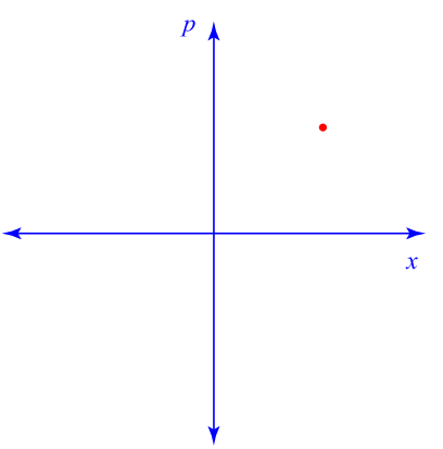
(a) An ontic state is a point in phase space.

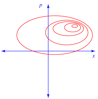
(b) An epistemic state is a probability density on phase space. Contours indicate lines of equal probability density.

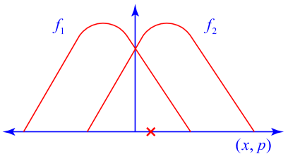
(c) An ontic state (cross) is deemed possible in more than one epistemic state ($f_{1}$ and $f_{2}$). Phase space has been schematically collapsed down to one dimension for illustrative purposes.

Figure 1: The distinction between ontic and epistemic states in single particle classical mechanics.

In classical mechanics, the distinction between ontic and epistemic states is fairly clear. A single Newtonian particle in one dimension has a position $x$ and a momentum $p$ and these are objective properties of the particle that exist independently of us. All other objective properties of the particle are functions of $x$ and $p$. The ontic state of the particle is therefore the phase space point $(x,p)$. This evolves according to Hamilton’s equations

$$\frac{dp}{dt} =-\frac{\partial H}{\partial x} \frac{dx}{dt} =\frac{\partial H}{\partial p},$$ (1)

where $H$ is the Hamiltonian. On the other hand, if we do not know the exact position and momentum of the particle then our knowledge about its ontic state is represented by a probability density $f(x,p)$ over phase space. By applying Hamilton’s equations to the individual phase space points on which $f(x,p)$ is supported, it can be shown that $f(x,p)$ evolves according to Liouville’s equation

$$\frac{\partial f}{\partial t}=\frac{\partial H}{\partial x}\frac{\partial f}{\partial p}-\frac{\partial H}{\partial p}\frac{\partial f}{\partial x}.$$ (2)

The probability density $f(x,p)$ is our epistemic state. See Fig. 1 for an illustration of the distinction between classical ontic and epistemic states. For other types of classical system the situation is analogous, the only difference being the dimension of the phase space, e.g. $6N$ dimensions for $N$ particles in $3$ dimensional space or a continuum for field systems. The phase space point is still the ontic state and a probability density over phase space is the epistemic state.

Note that calling a probability density “epistemic” is controversial in some circles. It presupposes a broadly Bayesian interpretation of probability theory in which probabilities represent an agent’s knowledge, information, or beliefs. Fortunately, the issue at stake does not really depend on this as it also appears in other interpretations of probability under a different name. What is important is that the states dubbed “epistemic” only have probabilistic import so they cannot be regarded as intrinsic properties of individual physical systems. The key property that this implies is that a given ontic state is deemed possible in more than one epistemic state.

On the Bayesian reading, this is due to the fact that different agents may have different knowledge about one and the same physical system. For example, perhaps Alice knows the position of a classical particle exactly but nothing about its momentum, whilst Bob knows the momentum precisely but nothing about its position. Alice and Bob would then assign different probability distributions to the system, with the crucial property that they would overlap on the ontic state actually occupied by the system.

Other interpretations of probability exhibit the same property in a different way. For example, on a frequentist account of probability, probabilities represent the relative frequencies of occurrence of some property in an ensemble of independently and identically prepared systems. In this context, we would talk about a state being “statistical” rather than “epistemic”. The statistical state of a system depends upon the choice of ensemble that the individual system is regarded as being a part of. For example, suppose a classical particle occupies the phase space point $(1\leavevmode\nobreak\ m,1\leavevmode\nobreak\ kgms^{-1})$. If we regard it as part of an ensemble of particles that all have positive position, but some have negative momentum, then it will be assigned a different probability distribution than if we regard it as part of an ensemble of particles all of which have positive momentum, but some have negative position. In the former case, the probability distribution will have support on negative momentum phase space points and in the latter case it will have support on negative position phase space points. The point is that ensembles consist of more than one individual system and the same ontic state may occur as a part of many different ensembles. A frequentist will not be lead astray by substituting the word “statistical” for every occurrence of the word “epistemic” in this article, but the latter terminology is used here because it has become standard.

Interpretations of probability that involve single-case objective chances present more of a challenge for the ontic/epistemic distinction, since they imply that probabilities can at least sometimes be ontic. Nevertheless, I believe that an appropriate distinction can still be made in most of these theories. This discussion is deferred to Appendix §A since it is mainly of interest to those concerned with the philosophy of probability. However, it is worth mentioning that many of those who have felt the need to introduce objective chances have been motivated in part by the role that probability plays in physics, and in quantum theory in particular. Since quantum probabilities are functions of the wavefunction, they only present a novel issue for the interpretation of probability if the wavefunction itself is ontic because only then would quantum probabilities need to have a more objective status than they do in classical physics. Since the status of the wavefunction is precisely the question at issue, it is perhaps wise to defer judgment on the necessity of objective chances until the reality of the wavefunction is decided.

What is at stake then is the following question: When a quantum state $\left|\psi\right\rangle$ is assigned to a physical system, does this mean that there is some independently existing property of the individual system that is in one-to-one correspondence with $\left|\psi\right\rangle$ (up to a global phase), or is $\left|\psi\right\rangle$ simply a mathematical tool for determining probabilities, existing only in the minds and calculations of quantum theorists? This is perhaps the most hotly debated issue in all of quantum foundations. I refer to it as the $\psi$-ontic/epistemic distinction and use the terms $\psi$-ontic/$\psi$-epistemic to describe interpretations that adopt an ontic/epistemic view of the quantum state. Holders of the $\psi$-ontic view have been dubbed $\psi$-ontologists by Christopher Granade (a masters student in Rob Spekkens’ quantum foundations course at Perimeter Institute in 2010) and, continuing in this vein, I refer to the reality of the quantum state as $\psi$-ontology and to theorems that attempt to establish this view as $\psi$-ontology theorems.

To avoid misunderstanding, note that the $\psi$-ontic/epistemic distinction is not about whether quantum states are ontic independently of whether quantum theory is exactly true. It is not about whether the ultimate final theory of physics, if indeed such a thing exists, will feature quantum states as part of its ontology. We have little idea of what such a final theory might look like and consequently we have little idea of what reality is actually made of at the most fundamental level. Nevertheless, we can still ask what quantum theory itself says about reality. In other words, we are imagining a hypothetical world in which quantum theory is in fact a completely correct theory of physics, and asking whether quantum states would have to be ontological in that world. That world is very unlikely to be our actual world, so the question is really about the internal structure of quantum theory. More specifically, it is about what kinds of explanation are compatible with quantum theory. For example, a $\psi$-ontic view implies that we should draw analogies between quantum states and phase space points when comparing quantum and classical physics, and between the Schrödinger equation and Hamilton’s equations, whereas a $\psi$-epistemic view says that the appropriate analogies are between quantum states and probability distributions, and between the Schrödinger equation and Liouville’s equation. If nothing else, this strongly impacts how we are to understand the classical limit of quantum theory (e.g. see [68, 69, 70, 71]). So, whilst the ontic/epistemic question may at first sight seem abstract and philosophical, it does in fact have concrete implications for physics.

The remainder of this part is structured as follows. §2 discusses arguments in favor of the $\psi$-epistemic view, with the aim of convincing you that $\psi$-ontology theorems are telling us something deep and surprising. For those that remain unconvinced, §3 reviews the main arguments for the reality of quantum states that were given prior to the discovery of $\psi$-ontology theorems. In my view, none of these are particularly compelling, so even someone who is already convinced of the reality of quantum states needs something like a $\psi$-ontology theorem if they aspire to defend their position with the same sort of conceptual force with which Bell derived nonlocality. Following this, §4 introduces the framework of ontological models, in which $\psi$-ontology theorems are proven, and gives the rigorous definition of the $\psi$-ontic/$\psi$-epistemic distinction. Finally, §5 discusses the implications of proving $\psi$-ontology, by showing that several existing no-go theorems can be derived from it.

2 Arguments for a $\psi$-epistemic interpretation

Before getting into the details of $\psi$-epistemic explanations, it is important to distinguish two kinds of $\psi$-epistemic interpretation. The most popular type are those variously described as anti-realist, instrumentalist, or positivist. Since these labels are often intended as terms of abuse, I prefer to call these approaches neo-Copenhagen in order to avoid implications for the philosophy of science that go way beyond how we choose to understand quantum theory. All such interpretations bear a family resemblance to the Copenhagen interpretation in that they are both $\psi$-epistemic and they deny the need for any deeper description of reality beyond quantum theory. Here, by “Copenhagen” I mean the views of Bohr, Heisenberg, Pauli et. al. (see e.g. [5]), which are clearly $\psi$-epistemic, rather than the view often found under this name in textbooks, which is actually due to Dirac [72] and von Neumann [73] and is more ambiguous about whether the wavefunction is real. If asked what quantum states represent knowledge about, neo-Copenhagenists are likely to answer that they represent knowledge about the outcomes of future measurements, rather than knowledge of some underlying observer-independent reality. Modern neo-Copenhagen views include the Quantum Bayesianism of Caves, Fuchs and Schack [16, 17, 18], the views of of Bub and Pitowsky [19], the quantum pragmatism of Healey [21], the relational quantum mechanics of Rovelli [22], the empiricist interpretation of W. M. de Muynck [23], as well as the views of David Mermin [24], Asher Peres [25], and Brukner and Zeilinger [26]. Some may quibble about whether all these interpretations resemble Copenhagen enough to be called neo-Copenhagen, but for present purposes all that matters is that these authors do not view the quantum state as an intrinsic property of an individual system and they do not believe that a deeper reality is required to make sense of quantum theory.

The second type of $\psi$-epistemic interpretation are those that are realist, in the sense that they do posit some underlying ontology. They just deny that the wavefunction is part of that ontology. Instead, the wavefunction is to be understood as representing our knowledge of the underlying reality, in the same way that a probability distribution on phase space represents our knowledge of the true phase space point occupied by a classical particle. There is evidence that Einstein’s view was of this type [74]. Ballentine’s statistical interpretation [75] is also compatible with this view in that he leaves open the possibility that hidden variables exist and only insists that, if they do exist, the wavefunction remains statistical (as a frequentist, Ballentine uses the term “statistical” rather than “epistemic”). More recently, Spekkens has been a strong advocate of this point of view [64].

Neo-Copenhagen and realist $\psi$-epistemic interpretations share much of the same explanatory structure, since they both view probability measures as the correct classical analogy for the wavefunction. Many of the arguments for adopting a $\psi$-epistemic interpretation apply equally to both of them. On the other hand, $\psi$-ontology theorems only apply to realist interpretations. This is to be expected as it would be difficult to prove that the wavefunction must be ontic in a framework that does not admit the existence of ontic states in the first place. Because of this, $\psi$-epistemicists always have the option of becoming neo-Copenhagen in the face of $\psi$-ontology theorems.

Realist $\psi$-epistemic interpretations are already strongly constrained by existing no-go theorems, such as Bell’s Theorem [1] and the Kochen–Specker Theorem [76], which go some way to explaining why not many concrete $\psi$-epistemic models have been proposed. However, there is no reason to view these results as decisive against realist $\psi$-epistemic interpretations any more than they are decisive against realist $\psi$-ontic interpretations. For example, Bohmian mechanics and spontaneous collapse theories still attract considerable support despite displaying nonlocality and contextuality, as the existing no-go theorems imply they must. Thus, we would be guilty of a double-standard if we ruled out realist $\psi$-epistemic interpretations on the basis of these results but still admitted the possibility of $\psi$-ontic ones. What is needed is a theorem that explicitly addresses the $\psi$-ontic/epistemic distinction, and this is the gap that $\psi$-ontology theorems are intended to fill.

In the remainder of this section, the main arguments in favor of $\psi$-epistemic interpretations are reviewed. Because we do not have a fully worked out realist $\psi$-epistemic model that covers the whole of quantum theory, it is helpful to introduce toy models that are similar to quantum theory in some respects, but in which the analogous notion to the quantum state is clearly epistemic. These are intended to demonstrate the kinds of explanation that are possible in $\psi$-epistemic theories. Spekkens’ toy theory [64], which reinvigorated interest in realist $\psi$-epistemic models in recent years, is reviewed in §2.1. There are also $\psi$-epistemic models that cover fragments of quantum theory, e.g. just pure state preparations and projective measurements of a single qubit or just continuous variable systems when restricted to Gaussian states and operations. These are reviewed in §2.2. Finally, I review three further arguments for the $\psi$-epistemic view based on the fact that quantum theory can be viewed as a generalization of classical probability theory in §2.3, on the collapse of the wavefunction in §2.4, and on the size of the quantum state space in §2.5.

2.1 Spekkens toy bit

Spekkens introduced a toy theory [64] that qualitatively reproduces the physics of spin-$1/2$ particles (or any other instantiation of qubits) when they are prepared and measured in the $x$, $y$ and $z$ bases. The full version of Spekkens theory incorporates dynamics and composite systems, including reproducing some of the phenomena associated with entangled states but, for illustrative purposes, we restrict attention to the simplest case of a single toy bit. The toy theory is meant to demonstrate the explanatory power of $\psi$-epistemic interpretations by providing natural explanations of many quantum phenomena that are puzzling if the quantum state is ontic.

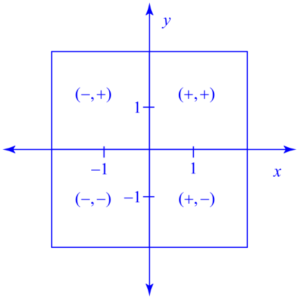
Figure 2: The ontic state space of Spekkens toy-bit. The ontic states are labeled $(x,y)$ where $x$ and $y$ take values $\pm 1$, which are abbreviated to $\pm$ for compactness.

A toy bit consists of a system that can be in one of four states, labeled $(-,-),(-,+),(+,-)$ and $(+,+)$. In Fig. 2, these are depicted laid out as a grid in the $x-y$ plane, with the origin lying at the center of the grid. The ontic states can then be thought of as representing the coordinates of the centers of the grid cells, given by $(x,y)$, with $\pm$ short for $\pm 1$. For concreteness, one can imagine that the cells of the grid represent four boxes and that the system is a ball that can be in one of them. The ontic state $(x,y)$ then represents the state of affairs in which the ball is in the box centered on the coordinates $(x,y)$.

The most fine grained description of the toy bit is always its ontic state, but we might not know exactly which of the ontic states is occupied. In general, our knowledge of the system is described by a probability distribution over the four ontic states, and this probability distribution is our epistemic state. Spekkens imagines that there is a restriction on the set of epistemic states that may be assigned to the system, called the knowledge-balance principle, which is in some ways analogous to the uncertainty principle. Roughly speaking, the knowledge balance principle states that at most half of the information needed to specify the ontic state can be known at any given time. This means, for example, that if we know the $x$-coordinate with certainty then we cannot know anything about the $y$-coordinate. Given this restriction, there are six possible states of maximal knowledge, termed pure states, as shown in the left hand side of Fig. 3. The pure states are denoted $\left|x\pm\right),\left|y\pm\right),\left|z\pm\right)$ in analogy to the quantum states $\left|x\pm\right\rangle,\left|y\pm\right\rangle,\left|z\pm\right\rangle$ of a spin-$1/2$ particle.

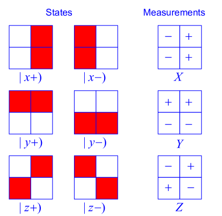
Figure 3: The allowed states and measurements of Spekkens’ toy bit. For the states, a red square indicates that the corresponding ontic state has probability $1/2$ and a white square indicates probability $0$. For the measurements, a square labeled $+$ gives the $+1$ outcome with certainty and a square labeled $-$ gives the $-1$ outcome with certainty.

Note that the epistemic states $\left|z\pm\right)$ are not states with a definite value of the $z$-coordinate. The system is two dimensional so it does not have a third coordinate. Instead, $\left|z+\right)$ is the state in which we know only that the $x$ and $y$ coordinates are equal and $\left|z-\right)$ is the state in which we know only that they are different. Defining $z=xy$, this is equivalent to saying that $\left|z\pm\right)$ is the state in which we know only that $z=\pm 1$.

Although the knowledge balance principle has been imposed by hand, it is easy to imagine that it could arise from a lack of fine-grained control over the system. For example, imagine a preparation device that pushes the ball to the left along the $x$-axis, but that same device also causes a random disturbance to the $y$-coordinate, such that the best we can do after operating the device is to assign the state $\left|x-\right)$.

Having described the epistemic states of the theory, the next task is to describe the measurements. Spekkens requires that measurements be repeatable, which means that if a measurement is repeated twice in succession then it should yield the same outcome both times. Also, the measurement should respect the knowledge balance principle, so that our epistemic state after the measurement contains at most half of the information required to specify the ontic state. In order to satisfy this second requirement, the measurement must necessarily cause a disturbance to the ontic state, since otherwise we could end up in a situation in which we know the ontic state exactly. For example, if a measurement of the $x$-coordinate could be implemented without disturbance then measuring the $x$-coordinate followed by measuring the $y$-coordinate would tell us the exact ontic state of the system.

There are three nontrivial measurements that can be implemented in such a way that they satisfy the two requirements: the $X$ measurement reveals the $x$ coordinate, the $Y$ measurement reveals the $y$ coordinate, and the $Z$ measurement reveals the value of $z=xy$. These are illustrated on the right hand side of Fig. 3. Each of these measurements causes a random exchange between the pairs of ontic states that give the same outcome in the measurement. For example, if we perform an $X$ measurement and get the $+1$ outcome, then with probability $1/2$ nothing happens and with probability $1/2$ the states $(+,-)$ and $(+,+)$ are exchanged. This ensures that we always end up in an epistemic state that satisfies the knowledge-balance principle at the end of the measurement, in this case $\left|x+\right)$. It is easy to see that this is the only type of disturbance that is compatible with both repeatability and the knowledge-balance principle. For example, for an $X$-measurement the random disturbance cannot exchange ontic states that have different values of the $x$-coordinate, e.g. $(+,+)$ and $(-,+)$, since this would violate repeatability.

The theory described so far makes exactly the same predictions as quantum theory for sequences of measurements in the $x$, $y$ and $z$ directions of spin-$1/2$ particles prepared in one of the states $\left|x\pm\right\rangle$, $\left|y\pm\right\rangle$ and $\left|z\pm\right\rangle$ if we identify these six states with $\left|x\pm\right)$, $\left|y\pm\right)$ and $\left|z\pm\right)$ and the Pauli observables $\sigma_{x}$, $\sigma_{y}$ and $\sigma_{z}$ with $X$, $Y$ and $Z$. It can thus be regarded as a hidden variable theory for this kind of experiment. Further, the quantum states are epistemic in this representation, as they are each represented by probability distributions that have support on two ontic states and nonorthogonal states overlap, e.g. $\left|x+\right)$ and $\left|y+\right)$ both assign probability $1/2$ to the ontic state $(+,+)$.

Several features of quantum theory that are puzzling on the $\psi$-ontic view are present in this theory and have very natural explanations. Firstly, consider the fact that nonorthogonal pure states cannot be perfectly distinguished by a measurement, e.g. if either the state $\left|x+\right\rangle$ or the state $\left|y+\right\rangle$ is prepared, and you do not know which, then there is no measurement that will enable you to deduce this information with certainty. If quantum states are ontic then the two preparations correspond to distinct states of reality and it is puzzling that we cannot detect this difference. On the other hand, the toy theory states $\left|x+\right)$ and $\left|y+\right)$ overlap on the ontic state $(+,+)$ and this will be occupied by the system $50\%$ of the time whenever $\left|x+\right)$ or $\left|y+\right)$ is prepared. When this does happen, there is nothing about the ontic state of the system that could possibly tell you whether $\left|x+\right)$ or $\left|y+\right)$ was prepared. Therefore, we must fail to distinguish the two preparations at least $50\%$ of the time. The overlap of the two epistemic states accounts for their indistinguishability.

Another feature of quantum theory that is easily accounted for in Spekkens’ model is the no-cloning theorem. In quantum theory, there is no transformation that copies both of two nonorthogonal states. For example, there is no device that operates with certainty and outputs both $\left|x+\right\rangle\otimes\left|x+\right\rangle$ when $\left|x+\right\rangle$ is input and $\left|y+\right\rangle\otimes\left|y+\right\rangle$ when $\left|y+\right\rangle$ is input. On the $\psi$-ontic view this is puzzling because the two states represent distinct states of reality, so one might expect that this distinctness could be detected and then copied over to another system. Again, this is easily explained in Spekkens’ model in terms of the overlap between the epistemic states $\left|x+\right)$ and $\left|y+\right)$. Fig. 4 shows the inputs and outputs of the hypothetical toy-theory cloning machine. The two input states overlap on the ontic state $(+,+)$ and this occurs $50\%$ of the time regardless of which input state is prepared. Since the cloning machine only has access to the ontic state, it must do the same thing to the state $(+,+)$, regardless of whether it occurs because $\left|x+\right)$ was prepared or because $\left|y+\right)$ was prepared. Therefore, $50\%$ of the time, the input must get mapped to the same set of ontic states, with the same probabilities, regardless of which state was prepared, so there must be at least a $50\%$ overlap of the output states of any physically possible device for these two input states. In contrast, the output states of the hypothetical cloning machine only overlap on the ontic state $((+,+),(+,+))$ and this must only occur $25\%$ of the time at the output for either input state. Therefore, the cloning machine is impossible.

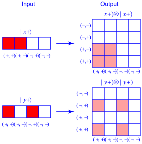
Figure 4: Inputs and outputs of a hypothetical toy bit cloning machine. In order to represent a two toy bit state, the ontic state space of a single toy bit is represented along one dimension. For the outputs, the horizontal axis represents the first toy bit and the vertical axis represents the second toy bit. Dark red represents ontic states occupied with $50\%$ probability and light red represents those occupied with $25\%$ probability. The inputs overlap on an ontic state that they both assign $50\%$ probability, but the outputs only overlap on an ontic state that they both assign $25\%$ probability.

In Spekkens’ toy theory, both indistinguishability and no-cloning follow from the more general fact that a stochastic map cannot decrease the overlap of two probability distributions. In quantum theory, there is a similar result that no transformation that can be implemented with certainty can decrease the inner product between two pure states [77]. This suggests that the inner product of two quantum states is analogous to the overlap between two probability distributions, and this analogy would be most easily explained if quantum states with nonzero inner product were literally represented by overlapping probability distributions on some ontic state space, i.e. by a realist $\psi$-epistemic interpretation.

Finally, consider the fact that mixed states in quantum theory have more than one decomposition into a convex sum of pure states. For example, the maximally mixed state of a spin-$1/2$ particle is $I/2$, where $I$ is the identity operator, and this can be written alternatively as

$$\frac{I}{2} =\frac{1}{2}\left|x+\right\rangle\left\langle x+\right|+\frac{1}{2}\left|x-\right\rangle\left\langle x-\right|$$ (3)

$$=\frac{1}{2}\left|y+\right\rangle\left\langle y+\right|+\frac{1}{2}\left|y-\right\rangle\left\langle y-\right|$$ (4)

$$=\frac{1}{2}\left|z+\right\rangle\left\langle z+\right|+\frac{1}{2}\left|z-\right\rangle\left\langle z-\right|.$$ (5)

Physically speaking, this means that if we prepare a spin-$1/2$ particle in the $\left|x+\right\rangle$ state with probability $1/2$ and in the $\left|x-\right\rangle$ state with probability $1/2$ then no experiment can tell the difference between this ensemble and that formed by preparing it in the $\left|y+\right\rangle$ state with probability $1/2$ and in the $\left|y-\right\rangle$ state with probability $1/2$ (and similarly for $\left|z\pm\right\rangle$). On a $\psi$-ontic view this is puzzling because the $\left|x\pm\right\rangle$ states are ontologically distinct from the $\left|y\pm\right\rangle$ (and $\left|z\pm\right\rangle$) states so this difference should be detectable. However, in Spekkens’ theory this non-uniqueness of decomposition is easily explained because preparing $\left|x+\right)$ with probability $1/2$ and $\left|x-\right)$ with probability $1/2$ leads to exactly the same distribution over ontic states as preparing $\left|y+\right)$ with probability $1/2$ and $\left|y-\right)$ with probability $1/2$ (and similarly for $\left|z\pm\right)$). This is illustrated in Fig. 5. Note that this is only possible because the distributions corresponding to nonorthogonal quantum states overlap.

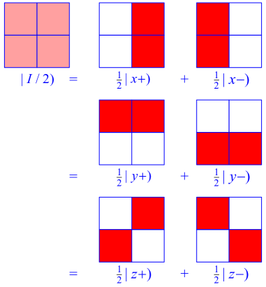
Figure 5: Multiple pure-state decompositions of a mixed state in Spekkens toy theory. The maximally mixed state $\left|I/2\right)$ can be written as a $50/50$ mixture in three different ways. Light red indicates a probability of $1/4$.

What has been presented in this section is just a small fraction of the quantum phenomena that are accounted for in Spekkens’ toy model. Many more can be found in [64], but I hope the present discussion has conveyed a flavor of the type of explanation that is possible in a realist $\psi$-epistemic theory.

2.2 Models for fragments of quantum theory

Spekkens’ toy model is qualitatively similar to the stabilizer fragment of quantum theory, which consists of the set of states that are joint eigenstates of maximal commutative subgroups of the Pauli group (i.e. the group generated by tensor products of the identity and the three Pauli operators) and has dynamics given by unitaries that map the Pauli group to itself (see [78] for details of the stabilizer formalism and [79] for a presentation of Spekkens’ toy theory that closely resembles it). The stabilizer fragment is important in quantum information theory as it contains all the states and operations needed for quantum error correction, as well as a number of other quantum protocols. Spekkens’ model does not exactly reproduce the stabilizer fragment when dynamics and entanglement are taken into account, but other models have been proposed that do reproduce fragments of quantum theory exactly in a $\psi$-epistemic manner.

First of all, Spekkens’ toy theory has been generalized to larger dimensions [65] and to continuous variable systems [66]. It turns out that for odd dimensional Hilbert spaces, Spekkens’ model reproduces the stabilizer fragment of quantum theory exactly. For continuous variable systems, Spekkens’ model reproduces the Gaussian fragment of quantum theory, in which all states are Gaussian and the transformations and measurements preserve the Gaussian nature of the states. A Gaussian state is one that has a Gaussian Wigner function. For a single particle, the Wigner function is defined in terms of the density operator $\rho$ as $W(x,p)=\int_{-\infty}^{+\infty}dse^{ips/\hbar}\left\langle x-\frac{s}{2}\right|\rho\left|x+\frac{s}{2}\right\rangle$ and is a pseudo-probability distribution, i.e. it is normalized to $1$ but it does not have to be positive. Gaussian functions are in fact positive so in this case $W(x,p)$ can be regarded as a probability distribution and unsurprisingly these are the epistemic states in Spekkens’ continuous variable theory, with the ontic states being the phase space points $(x,p)$.

Kochen and Specker gave a model for a single qubit that is $\psi$-epistemic [76]. They were not actually trying to generate a $\psi$-epistemic model, but rather to provide a counterexample to their eponymous theorem in $2$-dimensions in order to show that the theorem requires a Hilbert space of $\geq 3$ dimensions for its proof. Nevertheless, their model is a paradigmatic example of a $\psi$-epistemic theory. The details of this model are presented in §4.3 after we have introduced the formalism for realist $\psi$-epistemic models more rigorously. Along similar lines, Lewis et. al. [52] and Aaronson et. al. [53] have constructed $\psi$-epistemic models that work for all finite dimensional systems. These models were developed as technical counterexamples to certain conjectures about $\psi$-ontology theorems and as such they are not very elegant or plausible. They are discussed in context in §7.5.

2.3 Generalized probability theory

Apart from specific models, there are also qualitative arguments in favor of the $\psi$-epistemic view. The first of these is that quantum theory can be viewed as a noncommutative generalization of classical probability theory. Classically, consider the algebra $\mathcal{A}$ of random variables on a sample space under pointwise addition and multiplication. A probability distribution can then be regarded as a positive functional $\mu:\mathcal{A}\rightarrow\mathbb{R}$ that assigns to each random variable its expectation value. The quantum generalization of this is to replace the commutative algebra $\mathcal{A}$ by the noncommutative algebra $\mathfrak{B}\left(\mathcal{H}\right)$ of bounded operators on a Hilbert space $\mathcal{H}$. A quantum state $\rho$ is isomorphic to a positive functional $f_{\rho}$ on $\mathfrak{B}(\mathcal{H})$ given by $f_{\rho}(M)=\text{Tr}\left(M\rho\right)$. In fact, by a theorem of von Neumann [73], all positive linear functionals on $\mathfrak{B}\left(\mathcal{H}\right)$ that are normalized such that $f(I)=1$, where $I$ is the identity operator, are of this form.

Both $\mathcal{A}$ and $\mathfrak{B}\left(\mathcal{H}\right)$ are examples of von Neumann algebras, and a generalization of classical measure theoretic probability can be developed by defining generalized probability distributions to be positive normalized functionals on such algebras [80, 81]. This generalized theory has both classical probability theory and quantum theory as special cases. In this theory, quantum states are playing the same role in the quantum case that probability measures play in the classical case, and so it is natural to interpret quantum states and classical probabilities as the same kind of entity. Since classical probabilities are usually interpreted epistemically, it is natural to interpret quantum states in the same way.

This line of argument would not be too convincing if noncommutative probability theory were just a formal mathematical generalization with no practical applications. However, the theory has a rich array of applications in quantum statistical mechanics, and especially in quantum information theory. The full machinery of von Neumann algebras is not often needed in quantum information, as we are usually dealing with finite dimensional systems. Nevertheless, whenever the analogy is made between classical probability distributions and density operators, and between stochastic maps and quantum operations, generalized probability is at play in the background. For example, in quantum compression theory [82], a density operator on a finite Hilbert space is viewed as the correct generalization of a classical information source with finite alphabet, which would be described by a classical probability distribution. Similarly, a quantum channel is described by a quantum operation, and this is viewed as generalizing a classical channel, which would be modeled as a stochastic map.

In fact, it is difficult to find any area of quantum information and computing in which probabilities are not viewed as the correct classical analogs of quantum states, and this includes areas that concern themselves exclusively with pure states and unitary transformations. For example, the standard circuit model of quantum computing [83] only employs pure states and unitaries, but quantum computational complexity classes are most often defined as generalizations of classical probabilistic complexity classes (see [84] for definitions of the complexity classes mentioned in this section.). The class BQP, usually thought of as the set of problems that can be solved efficiently on a quantum computer, is sometimes loosely described as the quantum version of P, the class of problems that can be solved in polynomial time on a deterministic classical computer, but in fact it is the generalization of BPP, the set of problems that can be solved in polynomial time on a probabilistic classical computer with probability $>2/3$. All over quantum computing theory we find the analogy made to classical probabilistic computing, and not to classical deterministic computing.

It seems then, that if we take quantum information and computing seriously, we must take generalized probability theory seriously as well. On these and other grounds, I have argued elsewhere [85, 86] that quantum theory is indeed best viewed as a generalization of probability theory. The details of this would take us too far afield, but suffice to say there are good reasons for viewing quantum states as analogous to probability distributions and, if we do that, we should try to interpret them both in the same sort of way.

2.4 The collapse of the wavefunction

A straightforward resolution of the collapse of the wavefunction, the measurement problem, Schrödinger’s cat and friends is one of the main advantages of $\psi$-epistemic interpretations. Recall that the measurement problem stems from the fact that there are two different ways of propagating a quantum state forward in time. When the system is isolated and not being observed, the quantum state is evolved smoothly and continuously according to the Schrödinger equation. On the other hand, when a measurement is made on the system, the quantum state must be updated according to the projection postulate, leading to the instantaneous and discontinuous collapse of the wavefunction. Since a measurement is presumably just some type of physical interaction between system and apparatus, this poses the problem of why it is not also modeled by Schrödinger evolution. However, doing so leads to seemingly absurd situations, such as Schrödinger’s eponymous cat ending up in a superposition of being alive and dead at the same time.

The measurement problem is not so much resolved by $\psi$-epistemic interpretations as it is dissolved by them. It is revealed as a pseudo-problem that we were wrong to have placed so much emphasis on in the first place. This is because the measurement problem is only well-posed if we have already established that the quantum state is ontic, i.e. that it is a direct representation of reality. Only then does a superposition of dead and alive cats necessarily represent a distinct physical state of affairs from a definitely alive or definitely dead cat. On the other hand, if the quantum state only represents what we know about reality then the cat may perfectly well be definitely dead or alive before we look, and the fact that we describe it by a superposition may simply reflect the fact that we do not know which possibility has occurred yet.

2.5 Excess baggage

According to the $\psi$-ontologist, a single qubit contains an infinite amount of information because a pure state of a qubit is specified by two continuous complex parameters (ignoring normalization). For example, Alice could encode an arbitrarily long bit string as the decimal expansion of the amplitude of the $\left|0\right\rangle$ state. However, according to the Holevo bound [87], only a single bit of classical information can be encoded in a qubit in such a way that it can be reliably retrieved. If the quantum state truly exists in reality, it is puzzling that we cannot detect all of this extra information. Hardy has coined the term “ontological excess baggage” to refer to this phenomenon [61]. It seems that $\psi$-ontologists are attributing a lot more information to the state of reality than required to explain our observations.

The $\psi$-epistemic response to this is to note that a classical probability distribution is also specified by continuous parameters. A probability distribution over a single classical bit requires two real parameters (again ignoring normalization). If probabilities were intrinsic properties of individual systems then this would present a similar puzzle as there would be an infinite amount of information in a single bit. However, classical bits are in fact always either in the state zero or one and the probabilities simply represent our knowledge about that value. In reality, there is just as much information in a classical bit as we can extract from it, namely one bit. If the quantum state is epistemic, then the same resolution is available to the problem of excess baggage. The continuous parameters required to specify the state of a qubit simply represent our knowledge about it, and the actual ontic state of the qubit, whatever that may be, might only contain a finite amount of information.

The excess baggage problem is exacerbated by considering how the state space scales with the number of qubits. A pure state of $n$ qubits is specified by $2^{n}$ complex parameters, but only $n$ bits can be reliably encoded according to the Holevo bound. However, the number of parameters required to specify a probability distribution over $n$ bits also scales exponentially, so the $\psi$-epistemic resolution of the problem is still available.

In response to this, $\psi$-ontologists might be inclined to point out that the number of bits that can be reliably encoded in $n$ qubits depends on how exactly the communication task is defined. If Alice and Bob have pre-shared entanglement then Alice can send $2n$ bits to Bob in $n$ qubits via superdense coding [88]. Similarly, qubits perform better than classical bits in random access coding [89], wherein Bob is not required to reliably retrieve all of the bits that Alice sends, but only a limited number of them of his choice. However, the amount of information that Alice can send to Bob does not scale exponentially with the number of qubits in any of these protocols, so there is still an excess baggage problem.

3 Arguments for a $\psi$-ontic interpretation

Having reviewed the arguments in favor of $\psi$-epistemic interpretations, we now look at those that had been put forward in favor of the reality of quantum states prior to the discovery of $\psi$-ontology theorems. Despite receiving a good deal of support, I hope to convince you that they are far from compelling. Thus, even those who are already convinced of the reality of the quantum state should be interested in establishing their claim rigorously via $\psi$-ontology theorems.

A big difficulty in extracting arguments for $\psi$-ontology from the literature is that the majority of authors neglect the possibility of realist $\psi$-epistemic theories. Instead, they seem to think that either the wavefunction must be real, or else we must adopt some kind of neo-Copenhagen approach. Thus, many purported arguments for the reality of the wavefunction are really just arguments for the reality of something, regardless of whether that thing is the wavefunction. Since realist $\psi$-epistemic interpretations already accept the need for an objective reality, such arguments can be dismissed in the present context. From amongst these arguments, I have attempted to sift out those that say something more substantive about the wavefunction specifically. I have found four broad classes of argument, each of which is discussed in turn in this section. §3.1 discusses the argument from interference, §3.2 discusses the argument from the eigenvalue-eigenstate link, §3.3 discusses the argument from existing realist interpretations of quantum theory, and finally §3.4 discusses the argument from quantum computation.

3.1 Interference

We choose to examine a phenomenon which is impossible, absolutely impossible, to explain in any classical way, and which has in it the heart of quantum mechanics. In reality, it contains the only mystery. — R. P. Feynman [90] [Emphasis in original]

Following Feynman, single particle interference phenomena, such as the double slit experiment, are often viewed as containing the essential mystery of quantum theory. The problem of explaining the double slit experiment is usually presented as a dichotomy between explaining it in terms of a classical wave that spreads out and travels through both slits or in terms of a classical particle that travels along a definite trajectory that goes through only one slit. Neither of these explanations can account for both the interference pattern and the fact that it is built out of discrete localized detection events. A wave would not produce discrete detection events and a classical particle would not be affected by whether or not the other slit is open. This is taken as evidence that no classical description can work, and that something more Copenhagen-like must be at work.

Of course, the dichotomy between either classical waves or particles is a false one. If we allow the state of reality to be something more general, i.e. some sort of quantum stuff that we do not necessarily understand yet, then many additional explanations of the experiment become available. For example, there is the Bohmian picture in which both a wave and a particle exist, and the motion of the particle is guided by the wave. The wave then explains the interference fringes, whilst the particle explains the discrete detection events. This is by no means the only possibility, but it does highlight the gap in the usual argument. Nevertheless, in a realist picture, it seems that something wavelike needs to exist in order to explain the interference fringes, and the obvious candidate is the wavefunction.

However, in order to arrive at the conclusion that the wavefunction must be real, greater leeway has been given in determining what the ontic state might be like compared to the original argument, which intended to rule out both particles and waves. Given this, we should be careful to rule out other possibilities rigorously, rather than jumping to the conclusion that the wavefunction must be real. In this broader context, the only thing that the double slit experiment definitively establishes is that there must be some sort influence that travels through both slits in order to generate the interference pattern. It does not establish that this influence must be a wavefunction.

In fact, interference phenomena occur in some of the previously discussed $\psi$-epistemic models, so the inference from interference to the reality of the wavefunction is incorrect. In Spekkens’ toy theory, a notion of coherent superposition can be introduced such that, for example, $\left|y+\right)$ is a coherent superposition of $\left|x+\right)$ and $\left|x-\right)$. Such superpositions are preserved under dynamical evolution, so there is a superposition principle in the theory (see [64] for details). Further, since all two-dimensional Hilbert spaces are created equal, there is nothing special about the interpretation of the toy bit in terms of a spin-$1/2$ particle. It could equally well be a model of any other two-dimensional system. For example, consider the two dimensional subspace of an optical mode spanned by the vacuum state $\left|0\right\rangle$ and the state $\left|1\right\rangle$ where it contains one photon. The toy bit state $\left|x+\right)$ can be reinterpreted as $\left|0\right\rangle$ and $\left|x-\right)$ as $\left|1\right\rangle$, and by doing so a whole host of Mach-Zehnder interferometry experiments can be qualitatively reproduced by the theory [91]. This includes not only basic interferometry, but also such seemingly paradoxical effects as the delayed choice experiment [92] and the Elitzur-Vaidman bomb test [93]. In this theory, there is always a fact of the matter about which arm of the interferometer the photon travels along, but it does not fall afoul of the standard waves vs. particles argument because the vacuum state has structure. For example, the situation in which the photon travels along the left arm of a Mach-Zehnder interferometer would be represented in quantum theory by $\left|1\right\rangle_{L}\otimes\left|0\right\rangle_{R}$. The $\left|0\right\rangle_{R}$ factor would be represented by the epistemic state $\left|x+\right)$ in the toy theory, which is compatible with two possible ontic states $(+,+)$ and $(+,-)$, and these ontic states travel along the right arm of the interferometer. Hence, when a photon is in the left arm of an interferometer, and no photon is in the right arm, there is still a bit of information traveling along the right arm of the interferometer, corresponding to whether the ontic state is $(+,+)$ or $(+,-)$, that can be used to convey information about whether or not its path was blocked. There is an influence that travels through both arms, but that influence is not a wavefunction.

Interference phenomena also occur in all of the models discussed in §2.2 simply because they reproduce fragments of quantum theory exactly and those fragments contain coherent superpositions. It is arguable whether the mechanisms explaining interference in all these models are plausible, but the main point is that the direct inference from interference to the reality of the wavefunction is blocked by them. If there is an argument from interference to be made then it will need to employ further assumptions. Hardy’s $\psi$-ontology theorem, discussed in §9, can be viewed as an attempt at doing this, but, in light of the way that interference is modeled in Spekkens’ toy theory, its assumptions do not seem all that plausible.

Ultimately, the intuition behind the argument from interference stems from an analogy with classical fields. Because wavefunctions can be superposed, they exhibit interference. Prior to the discovery of quantum theory, the only entities in physics that obeyed a superposition principle and exhibited interference were classical fields, and these were definitely intended to be taken as real. For example, the value of the electromagnetic field at some point in space-time is an objective property that can be measured by observing the motion of test charges. The interference of wavefunctions is then taken as evidence that they should be interpreted as something similar to classical fields.

However, the analogy between wavefunctions and fields is only exact for a single spinless particle, for which the wavefunction is essentially just a field on ordinary three dimensional space. This breaks down for more than one particle, due to the possibility of entanglement. The size of the quantum state space scales exponentially with the number of systems, leading to the previously discussed excess baggage problem. The wavefunction can no longer be viewed as field on ordinary three-dimensional space, so the analogy with a classical field should be viewed with skepticism. In combination with the fact that interference phenomena can be modeled $\psi$-epistemically, the argument from interference is far from compelling.

3.2 The eigenvalue-eigenstate link

The eigenvalue-eigenstate link refers to the tenet of orthodox quantum theory that when a system is in an eigenstate $\left|m\right\rangle$ of an observable $M$ with eigenvalue $m$ then $M$ is a property of the system that has value $m$. Conversely, when the state is not an eigenstate of $M$ then $M$ is not a property of the system. In other words, the properties of a system consist of all the observables of which the quantum state is an eigenstate and nothing else. These properties are taken to be objectively real, independently of the observer.

This leads to an argument for the reality of the wavefunction because the quantum state of a system is determined uniquely by the set of observables of which it is an eigenstate. Indeed, it is determined uniquely by just a single observable, since $\left|\psi\right\rangle$ is an eigenstate of the projector $\left|\psi\middle\rangle\middle\langle\psi\right|$ with eigenvalue $1$ and (up to a global phase) it is the only state in the $+1$ eigenspace of $\left|\psi\middle\rangle\middle\langle\psi\right|$. The argument is then that, if a system has a set of definite properties, and those properties uniquely determine the wavefunction, then the wavefunction itself must be real.

Roger Penrose is perhaps the most prominent advocate of this argument, so here it is in his own words.

One of the most powerful reasons for rejecting such a subjective viewpoint concerning the reality of $\left|\psi\right\rangle$ comes from the fact that whatever $\left|\psi\right\rangle$ might be, there is always—in principle, at least–a primitive measurement whose YES space consists of the Hilbert space ray determined by $\left|\psi\right\rangle$. The point is that the physical state $\left|\psi\right\rangle$ (determined by the ray of complex multiples of $\left|\psi\right\rangle$) is uniquely determined by the fact that the outcome YES, for this state, is certain. No other physical state has this property. For any other state, there would merely be some probability, short of certainty, that the outcome will be YES, and an outcome of NO might occur. Thus, although there is no measurement which will tell us what $\left|\psi\right\rangle$ actually is, the physical state $\left|\psi\right\rangle$ is uniquely determined by what it asserts must be the result of a measurement that might be performed on it…

To put the point a little more forcefully, imagine that a quantum system has been set up in a known state, say $\left|\phi\right\rangle$, and it is computed that after a time $t$ the state will have evolved, under the action of $U$, into another state $\left|\psi\right\rangle$. For example, $\left|\phi\right\rangle$ might represent the state ‘spin up’ ($\left|\phi\right\rangle=\left|\uparrow\right\rangle$) of an atom of spin $\frac{1}{2}$, and we can suppose that it has been put in that state by the action of some previous measurement. Let us assume that our atom has a magnetic moment aligned with its spin (i.e. it is a little magnet pointing to the spin direction). When the atom is placed in a magnetic field, the spin direction will precess in a well-defined way, that can be accurately computed as the action of $U$, to give some new state, say $\left|\psi\right\rangle=\left|\rightarrow\right\rangle$, after a time $t$. Is this computed state to be taken seriously as part of physical reality? It is hard to see how this can be denied. For $\left|\psi\right\rangle$ has to be prepared for the possibility that we might choose to measure it with the primitive measurement referred to above, namely that whose YES space consists precisely of the multiples of $\left|\psi\right\rangle$. Here, this is the spin measurement in the direction $\rightarrow$. The system has to know to give the answer YES, with certainty for that measurement, whereas no spin state of the atom other than $\left|\psi\right\rangle=\left|\rightarrow\right\rangle$ could guarantee this. — Roger Penrose, quoted in [94].

This argument can be easily countered using any of the existing $\psi$-epistemic models, to which the same reasoning would apply. For example, consider the epistemic state $\left|x+\right)$ in Spekkens’ toy theory. This state assigns the definite value $+1$ to the $X$ measurement and indeed it is the only allowed epistemic state in the theory that does this. In fact, all of the pure states of a toy bit $\left|x\pm\right),\left|y\pm\right)$ and $\left|z\pm\right)$ are uniquely determined by the definite value that they assign to one of the measurements. Following Penrose’s reasoning, we would then conclude that these states are objective properties of the system. However, this is not the case since the objective properties of the system are those that are determined by the ontic state, and each ontic state is compatible with more than one epistemic state. For example, the ontic state $(+,+)$ is compatible with $\left|x+\right)$, $\left|y+\right)$ and $\left|z+\right)$. Given the complete specification of reality, the epistemic state is underdetermined.

One way of exposing the error in the eigenvalue-eigenstate argument is to note that, in the toy theory, the fact that observables uniquely determine epistemic states is a consequence of the knowledge-balance principle and not a fundamental fact about reality. For example, without the knowledge-balance principle, it would be permissible to have an epistemic state that assigns probability $2/3$ to $(+,+)$ and $1/3$ to $(+,-)$. Just like $\left|x+\right)$, this state assigns probability $1$ to the $+1$ outcome of the $X$ measurement and this is the only measurement that is assigned a definite value. If this state were allowed then it would no longer be possible to mistake $\left|x+\right)$ for an objective property of the system. Penrose has mistaken the set of states that it is possible to prepare with current experiments for the set of all logically possible states.

Another way of exposing the error is to look at the restrictions on measurements in the toy theory. The measurements only reveal coarse-grained information about the ontic state. Without the knowledge-balance principle it would be permissible to conceive of a more fine-grained measurement that reveals the ontic state exactly. This measurement reveals a definite property of the system because it is determined uniquely by the ontic state. However, specifying this observable no longer uniquely determines the epistemic state. For example, if we learn that the ontic state is $(+,+)$ then this is compatible with $\left|x+\right)$, $\left|y+\right)$ and $\left|z+\right)$.

In conclusion, the mistake in the eigenvalue-eigenstate argument is to assume that the observables that we can actually measure in experiments form the sum total of all the properties of the system and to assume that the set of states that we can actually prepare are the sum total of all logically conceivable states. Without these assumptions, the argument is simply false.

3.3 Existing realist interpretations

There are a handful of fully worked out realist interpretations of quantum theory, including many-worlds [6, 7, 8], de Broglie–Bohm theory [9, 10, 11, 12], spontaneous collapse theories [13, 14] and modal interpretations [15]. In each of these interpretations the wavefunction is part of the ontic state, so there is an argument from lack of imagination to be made: since all the interpretations of quantum theory that we have managed to come up with that are uncontroversially realist have a real wavefunction, then the wavefunction must be real.

I admit that it behooves the realist $\psi$-epistemicist to try to construct a fully worked out interpretation. However, absence of evidence is not the same thing as evidence of absence. Nevertheless, I have frequently heard this argument made in private conversations. Some people seem to think that since we have a bunch of well worked out interpretations, we ought to simply pick one of them and not bother thinking about other possibilities. Ever since the inception of quantum theory we have been beset by the problem of quantum jumps, by which I mean that quantum theorists are liable to jump to conclusions.

Despite the obvious weakness of this argument, there is a more subtle point to be made. John Bell was motivated to work on his eponymous theorem by noting that de Broglie–Bohm theory exhibited nonlocality. He wanted to know if this was just a quirk of de Broglie–Bohm theory or an inescapable property of any realist interpretation of quantum theory. With this motivation, he ended up proving the latter. The lesson of this is that if we find that all realist interpretations of quantum theory share a property that some find objectionable then we ought to determine whether or not this is a necessary property. However, this is a motivation for developing $\psi$-ontology theorems, rather than regarding the matter as settled a priori.

3.4 Quantum computation

The final argument I want to consider is due to David Deutsch, who put it forward as an argument in favor of the many-worlds interpretation. However, I think the argument can be adapted, more generally, into an argument for the reality of the wavefunction. Here is the argument in Deutsch’s own words.

To predict that future quantum computers, made to a given specification, will work in the ways I have described, one need only solve a few uncontroversial equations. But to explain exactly how they will work, some form of multiple-universe language is unavoidable. Thus quantum computers provide irresistible evidence that the multiverse is real. One especially convincing argument is provided by quantum algorithms […] which calculate more intermediate results in the course of a single computation than there are atoms in the visible universe. When a quantum computer delivers the output of such a computation, we shall know that those intermediate results must have been computed somewhere, because they were needed to produce the right answer. So I issue this challenge to those who still cling to a single-universe world view: if the universe we see around us is all there is, where are quantum computations performed? I have yet to receive a plausible reply. — David Deutsch [95] [Emphasis in original].

Quantum algorithms that offer exponential improvement over existing classical algorithms, such as Shor’s factoring algorithm [96], start by putting a quantum system in a superposition of all possible input strings. Then, some computation is done on each of the strings before using interference effects between them to elicit the answer to the computation. If each of the branches of the wavefunction were not individually real, whether or not they are interpreted in a many-worlds sense, then where does the computation get done?

This is not exactly an argument for the reality of the wavefunction, but it is at least an argument that the size of ontic state space should scale exponentially with the number of qubits, and that the ontic state should contain pieces that look like the branches of a wavefunction. However, whilst I agree with Deutsch that an interpretation of quantum theory should offer an explanation of how quantum computations work, it is not at all obvious that the explanation must be a direct translation of what happens to the wavefunction. The argument would perhaps be more compelling if there were known exponential speedups for problems where we think that the best we can do classically is to just search through an exponentially large set of solutions, since we could then argue that a quantum computer must be doing just that. This would be the case if we had such a speedup for the traveling salesman problem, or any other NP complete problem. The sort of problems for which we do have exponential speedup, such as factoring, are more subtle than this. They lie in NP, but are not NP complete. If we were to find an efficient classical algorithm for these problems then it would not cause the whole structure of computational complexity theory to come crashing down. If such an algorithm exists, then whatever deeper theory underlies quantum theory may be exploiting this same structure to perform the quantum computation.

Even if such a scenario does not play out, Deutsch’s argument is not decisive against realist $\psi$-epistemic interpretations. Since we have not yet constructed a viable interpretation of this sort that covers the whole of quantum theory, who knows what explanations such a theory might provide? Therefore, as Deutsch says, explaining quantum computation ought to be viewed as a challenge for the $\psi$-epistemic program rather than an argument against it.

4 Formalizing the $\psi$-ontic/epistemic distinction

Hopefully, by this point I have convinced you that it is worth trying to settle the question of the reality of the wavefunction rigorously. The aim of this section is to provide a formal definition of what it means for the quantum state to be ontic or epistemic within a realist model of quantum theory. This is usually done within the framework of ontological models. This is really no different from the framework that Bell used to prove his eponymous theorem, and an ontological model is sometimes alternatively known as a hidden variable theory. However, I prefer the term “ontological model” because there is a lot of confusion about the meaning of the term “hidden variables”. Following the example of Bohmian mechanics, a hidden variable theory is often thought to be a theory in which some additional variables are posited alongside the wavefunction, which is itself conceived of as ontic from the start. Since the reality of the wavefunction is precisely the point at issue, we definitely want to include models in which it is not assumed to be real within our framework. In addition, in order to cover orthodox quantum theory, we want our framework to include models in which the wavefunction is the only thing that is real, i.e. there are no additional hidden variables. A further confusion is the commonly held view that a hidden variable theory must restore determinism, whereas we want to allow for the possibility that nature might be genuinely stochastic. For these reasons, I prefer to use the term “ontological model”. It is either the same thing as a hidden variable theory or more general, depending on how general you thought hidden variable theories were in the first place.

Whilst the Hardy and Colbeck–Renner Theorems involve assumptions about how dynamics are represented in an ontological model, the Pusey–Barrett–Rudolph Theorem only involves prepare-and-measure experiments, i.e. a system is prepared in some quantum state and is then immediately measured and discarded. Therefore, we deal with prepare-and-measure experiments first and defer discussion of dynamics until it is needed. A $\psi$-ontology theorem aims at proving that any ontological model that reproduces quantum theory must have ontic quantum states. This does not apply to arbitrary fragments of quantum theory, since we have seen in §2.2 that there are fragments that can be modeled with epistemic quantum states. In order to understand both cases, we need to define ontological models for fragments of quantum theory rather than just for quantum theory as a whole. The formal definition of a prepare-and-measure fragment of quantum theory is given in §4.1 and then §4.2 explains how these are represented in ontological models, with examples given in §4.3. Based on this, §4.4 gives the formal definition of what it means for the quantum state to be ontic or epistemic.

4.1 Prepare and measure experiments

In a prepare-and-measure experiment, the experimenter performs a preparation of some physical system and then immediately measures it, records the outcome, and discards the system. The experimenter can repeat the whole process of preparing and measuring as many times as she likes in order to build up frequency statistics for comparison with the probabilities predicted by some physical theory. Each run of the experiment is assumed to be statistically independent of the others and it is assumed that the experimenter can choose which measurement to perform independently of the choice of preparation.

For completeness, we consider the most general type of quantum state—a density operator—and the most general type of observable —a Positive Operator Valued Measure (POVM), although we restrict attention to POVMs with a finite number of outcomes. Readers unfamiliar with these concepts should consult a standard textbook, such as [83] or [97].

Definition 4.1.

A prepare-and-measure (PM) fragment $\mathfrak{F}=\langle\mathcal{H},\mathcal{P},\mathcal{M}\rangle$ of quantum theory consists of a Hilbert space $\mathcal{H}$, a set $\mathcal{P}$ of density operators on $\mathcal{H}$, and a set $\mathcal{M}$ of POVMs on $\mathcal{H}$. The probability of obtaining the outcome corresponding to a POVM element $E\in M$ when performing a measurement $M\in\mathcal{M}$ on a system prepared in the state $\rho\in\mathcal{P}$ is given by the Born rule

$$\text{Prob}(E|\rho,M)=\text{Tr}\left(E\rho\right).$$ (6)

For many of the results reviewed here, the PM fragment under consideration is the one in which $\mathcal{P}$ is the set of all pure states on $\mathcal{H}$ and $\mathcal{M}$ consists of measurements in a set of complete orthonormal bases. The formalism of PM fragments allows the sets of states and measurements required to make $\psi$-ontology theorems go through to be made explicit. Additionally, many of the intermediate results used in proving $\psi$-ontology theorems apply to PM fragments in general, including those that feature mixed states and POVMs, so it is worth introducing fragments at this level of generality.

When only a single PM fragment is under consideration, it is assumed to be denoted $\langle\mathcal{H},\mathcal{P},\mathcal{M}\rangle$ so that the notations $\rho\in\mathcal{P}$ and $M\in\mathcal{M}$ can be used without first explicitly writing down the triple.

4.2 Ontological models

The idea of an ontological model of a PM fragment is that there is some set $\Lambda$ of ontic states that give a complete specification of the properties of the physical system as they exist in reality. When a quantum system is prepared in a state $\rho\in\mathcal{P}$, what really happens is that the system occupies one of the ontic states $\lambda\in\Lambda$. However, the preparation procedure may not completely control the ontic state, so our knowledge of the ontic state is described by a probability measure $\mu$ over $\Lambda$. This means that $\Lambda$ needs to be a measurable space, with a $\sigma$-algebra $\Sigma$, and that $\mu:\Sigma\rightarrow[0,1]$ is a $\sigma$-additive function satisfying $\mu(\Lambda)=1$. For those unfamiliar with measure-theoretic probability, for a finite space $\Sigma$ would just be the set of all subsets of $\Lambda$ and $\sigma$-additivity reduces to $\mu(\Omega_{1}\cup\Omega_{2})=\mu(\Omega_{1})+\mu(\Omega_{2})$ for all disjoint subsets $\Omega_{1}$ and $\Omega_{2}$ of $\Lambda$.

In general, different methods of preparing the same quantum state may result in different probability measures over the ontic states. This is especially true of mixed states, since they do not have unique decompositions into a convex mixture of pure states. If one prepares a mixed state by choosing randomly from one of the pure states in such a decomposition, then one can prove that the probability measure must in general depend on the choice of decomposition. This is known as preparation contextuality, and is discussed in more detail in §5.3. For this reason, a quantum state $\rho$ is associated with a set $\Delta_{\rho}$ of probability measures rather than just a single unique measure. Note that it is possible to find models in which pure states correspond to unique measures, and much of the literature implicitly assumes this type of model. However, it turns out that this assumption is not necessary, so we allow for the possibility that even a pure state is represented by a set of probability measures for the sake of generality.

Turning now to measurements, the outcome of a measurement $M\in\mathcal{M}$ might not reveal $\lambda$ exactly but depend on it only probabilistically. This could be because nature is fundamentally stochastic, but it could also arise in a deterministic theory if the response of the measuring device depends not only on $\lambda$ but also on degrees of freedom within the measuring device that are not under the experimenter’s control (see [98] for a discussion of this). To account for this, each POVM $M$ is represented by a conditional probability distribution $\text{Pr}(E|M,\lambda)$ over $M$. In a bit more detail, when a measurement $M\in\mathcal{M}$ is performed, each $\lambda$ must give rise to a well defined probability distribution over the outcomes, so, for any fixed $\lambda$, we must have $\text{Pr}(E|M,\lambda)\geq 0$ for all $E\in M$ and $\sum_{E\in M}\text{Pr}(E|M,\lambda)=1$. Further, in order to calculate the probabilities that the model predicts we will observe, we are going to have to average over our ignorance about $\lambda$ so, for any fixed $E$, $\text{Pr}(E|M,\lambda)$ must be a measurable function of $\lambda$. See Fig. 6 for an illustration of the conditional probability distribution corresponding to a measurement.

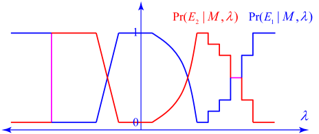
Figure 6: A possible conditional probability distribution $\text{Pr}(E_{j}|M,\lambda)$ for a two outcome measurement $M=\{E_{1},E_{2}\}$ in an ontological model. $\text{Pr}(E_{j}|M,\lambda)$ is the conditional probability of obtaining the outcome $E_{j}$ when $M$ is measured and the ontic state is $\lambda$. As a result, it must satisfy $\text{Pr}(E_{1}|M,\lambda)+\text{Pr}(E_{2}|M,\lambda)=1$ for all values of $\lambda$. For illustrative purposes, the ontic state space is represented as a $1$-dimensional line, but it may actually be an arbitrary measurable space.

Again, different methods of implementing the same measurement may result in different conditional probability distributions. This is known as measurement contextuality and it must occur in certain types of model due to the Kochen–Specker theorem [76]. Measurement contextuality is discussed further in Appendix C. For this reason, a measurement $M$ is associated with a set $\Xi_{M}$ of conditional probability distributions rather than just a single one.

In order to compute the probabilities that the ontological model predicts for the observable outcomes of measurements, the conditional probabilities $\text{Pr}(E|M,\lambda)$ have to be averaged over our ignorance of the true ontic state as specified by $\mu$. This gives,

$$\text{Pr}(E|\rho,M)=\int_{\Lambda}\text{Pr}(E|M,\lambda)d\mu(\lambda).$$ (7)

Note that, the notation Pr is used for the probabilities in an ontological model to distinguish them from the probabilities Prob predicted by quantum theory.

Finally, if the ontological model is to reproduce the predictions of quantum theory, then; for each $\rho\in\mathcal{P}$, $M\in\mathcal{M}$, each $\mu\in\Delta_{\rho}$, $\text{Pr}\in\Xi_{M}$ must satisfy

$$\text{Pr}(E|\rho,M)=\text{Prob}(E|\rho,M),$$ (8)

or in other words

$$\int_{\Lambda}\text{Pr}(E|M,\lambda)d\mu(\lambda)=\text{Tr}\left(E\rho\right).$$ (9)

Summarizing, we have

Definition 4.2.

An ontological model of a PM fragment is a quadruple $(\Lambda,\Sigma,\Delta,\Xi)$ that consists of:

• A measurable space $(\Lambda,\Sigma)$, where $\Lambda$ is called the ontic state space.

• A function $\Delta$ that maps each quantum state $\rho\in\mathcal{P}$ to a set of probability measures $\Delta[\rho]=\Delta_{\rho}$ on $(\Lambda,\Sigma)$.

• A function $\Xi$ that maps each POVM $M\in\mathcal{M}$ to a set of conditional probability distributions over $M$, $\Xi[M]=\Xi_{M}$, i.e. each $\text{Pr}\in\Xi_{M}$ is a function from $M\times\Lambda$ to $\mathbb{R}$ that is measurable as a function of $\lambda\in\Lambda$ and satisfies, for all $\lambda\in\Lambda$,

  $$\forall E\in M,\,\,\,\,\text{Pr}(E|M,\lambda)\geq 0$$ (10)

  and

  $$\sum_{E\in M}\text{Pr}(E|M,\lambda)=1.$$ (11)

The ontological model reproduces the quantum predictions if, for all $\rho\in\mathcal{P}$ and $M\in\mathcal{M}$, each $\mu\in\Delta_{\rho}$ and $\text{Pr}\in\Xi_{M}$ satisfies

$$\forall E\in M,\,\,\,\,\int_{\Lambda}\text{Pr}(E|M,\lambda)d\mu(\lambda)=\text{Tr}\left(E\rho\right).$$ (12)

In what follows, it is convenient to use projectors $\left|\psi\middle\rangle\middle\langle\psi\right|$ to represent pure states instead of vectors $\left|\psi\right\rangle$ to avoid the global phase ambiguity. The set of projectors onto the pure states of $\mathcal{H}$ is known as the projective Hilbert space of $\mathcal{H}$. The notation $\left[\psi\right]=\left|\psi\middle\rangle\middle\langle\psi\right|$ and $\Delta_{\psi}=\Delta_{\left[\psi\right]}$ is used to reduce clutter. Similarly, if a measurement $M$ consists of projectors onto pure states $\left[\phi\right]$ then we use the notation $\text{Pr}(\phi|M,\lambda)$ as shorthand for $\text{Pr}(\left[\phi\right]|M,\lambda)$.

4.3 Examples of Ontological Models

Example 4.3 (Spekkens’ toy bit).

Spekkens’ toy bit can be recast as an ontological model of the PM fragment $\langle\mathbb{C}^{2},\mathcal{P},\mathcal{M}\rangle$ where

$$\mathcal{P}=\left\{\left[x+\right],\left[x-\right],\left[y+\right],\left[y-\right],\left[z+\right],\left[z-\right],I/2\right\},$$ (13)

and

$$\mathcal{M}=\left\{\left\{\left[x+\right],\left[x-\right]\right\},\left\{\left[y+\right],\left[y-\right]\right\},\left\{\left[z+\right],\left[z-\right]\right\}\right\}.$$ (14)

The ontic state space is $\Lambda=\{(+,+),(+,-),(-,+),(-,-)\}$. Since $\Lambda$ is a finite set, the integral in Eq. (12) is just a sum

$$\sum_{\lambda\in\Lambda}\text{Pr}(E|M,\lambda)\mu(\lambda)=\text{Tr}\left(E\rho\right),$$ (15)

where, abusing notation slightly, we write $\mu(\lambda)$ for $\mu(\{\lambda\})$.

In this model, each quantum state is represented by a unique probability measure. The six probability functions $\left|x\pm\right),\left|y\pm\right),\left|z\pm\right)$ illustrated in Fig. 3 represent the states $\left[x\pm\right],\left[y\pm\right],\left[z\pm\right]$, and $\left|I/2\right)$ from Fig. 5 represents the maximally mixed state $I/2$. Each measurement is associated with a unique conditional probability distribution as described in Fig. 3. For example, for the $X=\{\left[x+\right],\left[x-\right]\}$ measurement we have

$$\begin{array}[]{lllll}\text{Pr}(x+|X,(+,+))&=&\text{Pr}(x+|X,(+,-))&=&1\\ \text{Pr}(x+|X,(-,+))&=&\text{Pr}(x+|X,(-,-))&=&0\\ \text{Pr}(x-|X,(+,+))&=&\text{Pr}(x-|X,(+,-))&=&0\\ \text{Pr}(x-|X,(-,+))&=&\text{Pr}(x-|X,(-,-))&=&1.\end{array}$$ (16)

It is easy to check that this reproduces the quantum predictions for the fragment.

Example 4.4 (The Beltrametti–Bugajski model [99]).

This model is essentially a translation of the orthodox interpretation of quantum theory into the language of ontological models. The PM fragment is $\langle\mathbb{C}^{d},\mathcal{P},\mathcal{M}\rangle$ where $\mathcal{P}$ contains all the pure states on $\mathbb{C}^{d}$ and $\mathcal{M}$ consists of all POVMs on $\mathbb{C}^{d}$. The idea of the model is that the quantum state, and only the quantum state, represents reality. Therefore, the ontic state space $\Lambda$ is just the set of pure states $\left[\lambda\right]$ for $\left|\lambda\right\rangle\in\mathbb{C}^{d}$, i.e. states differing by a global phase are identified so $\Lambda$ is the projective Hilbert space of $\mathbb{C}^{d}$. This space carries a natural topology induced by the inner product, and we take $\Sigma$ to be the Borel $\sigma$-algebra of this topology (see [100] for details).

A pure quantum state $\left[\psi\right]$ is then represented by the point measure

$$\mu(\Omega)=\delta_{\psi}(\Omega)=\begin{cases}1&\text{if}\,\,\left[\psi\right]\in\Omega\\ 0&\text{if}\,\,\left[\psi\right]\notin\Omega.\end{cases}$$ (17)

Each POVM is represented by a unique conditional probability distribution and, since the quantum state is the ontic state in this model, it should come as no surprise that the response functions simply specify the quantum probabilities, i.e. if a POVM $M\in\mathcal{M}$ contains the operator $E$ then

$$\text{Pr}(E|M,\left[\lambda\right])=\text{Tr}\left(E\left[\lambda\right]\right).$$ (18)

We then trivially have

$$\int_{\Lambda}\text{Pr}(E|M,\left[\lambda\right])d\mu(\left[\lambda\right]) = \int_{\Lambda}\text{Tr}\left(E\left[\lambda\right]\right)d\delta_{\psi}(\left[\lambda\right])$$ (19)

$$= \text{Tr}\left(E\left[\psi\right]\right),$$

so the model reproduces the quantum predictions.

The model can be extended to mixed states by writing them as convex combinations of pure states. For example, the maximally mixed state of a spin-$1/2$ particle can be written as

$$\frac{I}{2}=\frac{1}{2}\left[x+\right]+\frac{1}{2}\left[x-\right].$$ (20)

This means that $I/2$ can be prepared by flipping a coin, preparing $\left[x+\right]$ if the outcome is heads or $\left[x-\right]$ if the outcome is tails, and then forgetting or erasing the result of the coin flip. Let’s call this preparation procedure $P$. It follows that the predictions of $I/2$ can be reproduced by the measure

$$\mu=\frac{1}{2}\delta_{x+}+\frac{1}{2}\delta_{x-}.$$ (21)

Note however that this is a preparation contextual model because the maximally mixed state can also be prepared by mixing a different set of pure states, e.g. the decomposition

$$\frac{I}{2}=\frac{1}{2}\left[y+\right]+\frac{1}{2}\left[y-\right],$$ (22)

yields the measure

$$\mu=\frac{1}{2}\delta_{y+}+\frac{1}{2}\delta_{y-},$$ (23)

which reproduces the quantum predictions just as well. In general, $\Delta_{\rho}$ consists of one convex combination of point measures for each of the different ways of writing $\rho$ as a mixture of pure states.

Example 4.5 (The Bell Model [101]).

In his review of no-go theorems for hidden variable theories [101], Bell introduced an ontological model for measurements in orthonormal bases on systems with a two-dimensional Hilbert space. The obvious generalization to arbitrary finite dimensional systems is presented here, as it is needed in §7.5. Bell intended his model as a pedagogical device to point out the flaws in previous no-go theorems, and he was primarily interested in whether a deterministic theory could reproduce the quantum predictions. In modern terms, the Bell model can be thought of as a minimal modification of the Beltrametti–Bugajski model, intended to make it deterministic.

The PM fragment of interest is $\mathfrak{F}=\langle\mathbb{C}^{d},\mathcal{P},\mathcal{M}\rangle$, where $\mathcal{P}$ consists of all pure states and $\mathcal{M}$ consists of all measurements of the form $\mathcal{M}=\left\{\left[\phi_{j}\right]\right\}_{j=0}^{d-1}$, where $\left\{\left|\phi_{j}\right\rangle\right\}_{j=0}^{d-1}$ is an orthonormal basis for $\mathbb{C}^{d}$.

The generalized Bell model employs an ontic state space $\Lambda=\Lambda_{1}\times\Lambda_{2}$ that is the Cartesian product of two state spaces. As in Beltrametti–Bugajski, $\Lambda_{1}$ is the projective Hilbert space of $\mathbb{C}^{d}$, with Borel $\sigma$-algebra $\Sigma_{1}$. $\Lambda_{2}$ is the unit interval $[0,1]$, with Borel $\sigma$-algebra $\Sigma_{2}$, representing an additional hidden variable. The measurable space is then $(\Lambda_{1}\times\Lambda_{2},\Sigma_{1}\otimes\Sigma_{2})$, where the tensor product $\sigma$-algebra $\Sigma_{1}\otimes\Sigma_{2}$ is the $\sigma$-algebra generated by sets of the form $\Omega_{1}\times\Omega_{2}$ with $\Omega_{1}\in\Sigma_{1}$, $\Omega_{2}\in\Sigma_{2}$.

The quantum state $\left[\psi\right]$ is represented by a product measure

$$\mu(\Omega)=\int_{\Lambda_{2}}\mu_{1}(\Omega_{\lambda_{2}})d\mu_{2}(\lambda_{2}),$$ (24)

where $\mu_{1}$ and $\mu_{2}$ are probability measures on $\Lambda_{1}$ and $\Lambda_{2}$ respectively, $\Omega\in\Sigma_{1}\otimes\Sigma_{2}$, and

$$\Omega_{\lambda_{2}}=\left\{\left[\lambda_{1}\right]\in\Lambda_{1}\middle|\left(\left[\lambda_{1}\right],\lambda_{2}\right)\in\Omega\right\}.$$ (25)

As in the Beltrametti–Bugajski model, $\left[\lambda_{1}\right]$ represents the quantum state so $\mu_{1}=\delta_{\psi}$. The other variable $\lambda_{2}$ is uniformly distributed so $\mu_{2}$ is just the uniform measure on $[0,1]$.

The outcome of a measurement $M=\{\left[\phi_{j}\right]\}_{j=0}^{d-1}$ is determined as follows. For each $\left[\lambda_{1}\right]$, the unit interval is divided into $d$ subsets of length $\text{Tr}\left(\left[\phi_{j}\right]\left[\lambda_{1}\right]\right)$. If $\lambda_{2}$ is in the subset corresponding to $\left[\phi_{j}\right]$ then the $\left[\phi_{j}\right]$ outcome occurs with certainty. It does not matter how we choose the subsets so long as they are disjoint and of the right length. One way of doing it is to pick the $j$th set to be the interval

$$\sum_{k=0}^{j-1}\text{Tr}\left(\left[\phi_{k}\right]\left[\lambda_{1}\right]\right)\leq\lambda_{2}<\sum_{k=0}^{j}\text{Tr}\left(\left[\phi_{k}\right]\left[\lambda_{1}\right]\right),$$ (26)

as illustrated in Fig. 7.

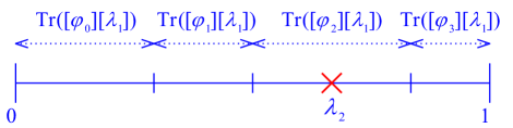
Figure 7: Example of the conditional probabilities in the Bell model for a measurement in $\mathbb{C}^{4}$. The unit interval is divided into $4$ subintervals of length $\text{Tr}\left(\left[\phi_{j}\right]\left[\lambda_{1}\right]\right)$. If $\lambda_{2}$ is in the $j$th interval then the outcome will be $j$. In the case depicted, the outcome is $\left[\phi_{2}\right]$.

This corresponds to the conditional probabilities

$$\text{Pr}(\phi_{j}|M,\left[\lambda_{1}\right],\lambda_{2})=\begin{cases}1&\text{if}\,\,\begin{array}[]{c}\sum_{k=0}^{j-1}\limits\text{Tr}\left(\left[\phi_{k}\right]\left[\lambda_{1}\right]\right)\leq\lambda_{2};\\ \lambda_{2}<\sum_{k=0}^{j}\limits\text{Tr}\left(\left[\phi_{k}\right]\left[\lambda_{1}\right]\right)\end{array}\\ 0&\text{otherwise}.\end{cases}$$ (27)

Note that, in this model, measurement-outcome pairs represented by the same projector generally correspond to different response functions. This is because the way that the unit interval is divided up depends on which other projectors are present in $\{\left[\phi_{j}\right]\}_{j=0}^{d-1}$. This is an example of measurement contextuality.

It is straightforward to see that this model reproduces the quantum predictions. If the state prepared is $\left[\psi\right]$ then the point measure $\mu_{1}$ implies that $\left[\lambda_{1}\right]=\left[\psi\right]$. Therefore, the length of the $j$th subset of the unit interval will be $\text{Tr}\left(\left[\phi_{j}\right]\left[\psi\right]\right)$. Since $\mu_{2}$ is the uniform measure on $[0,1]$, the probability of $\lambda_{2}$ being in a subset of $[0,1]$ is just the total length of the subset, so the observed probability of obtaining outcome $j$ is $\text{Tr}\left(\left[\phi_{j}\right]\left[\psi\right]\right)$, as required.

Example 4.6 (The Kochen–Specker model [76]).

Kochen and Specker introduced an ontological model for measurements in orthonormal bases on a two-dimensional system. The PM fragment is $\langle\mathbb{C}^{2},\mathcal{P},\mathcal{M}\rangle$ where $\mathcal{P}$ consists of all pure states on $\mathbb{C}^{2}$ and $\mathcal{M}$ consists of all measurements of the form $M=\{\left[\phi\right],\left[\phi^{\perp}\right]\}$ with $\{\left|\phi\right\rangle,\left|\phi^{\perp}\right\rangle\}$ an orthonormal basis.

A pure state $\left[\psi\right]$ in a two dimensional Hilbert space can be represented as a point $\vec{\psi}=(\sin\vartheta\cos\varphi,\sin\vartheta\sin\varphi,\allowbreak\cos\vartheta)$ on the surface of a unit $2$-sphere $S_{2}$ by choosing a representative vector $\left|\psi\right\rangle$ via

$$\left|\psi\right\rangle=\cos(\frac{\vartheta}{2})\left|z+\right\rangle+e^{\imath\varphi}\sin(\frac{\vartheta}{2})\left|z-\right\rangle,$$ (28)

where $0\leq\vartheta<\pi$ and $-\pi<\varphi\leq\pi$. This is known as the Bloch sphere representation (see Fig. 8).

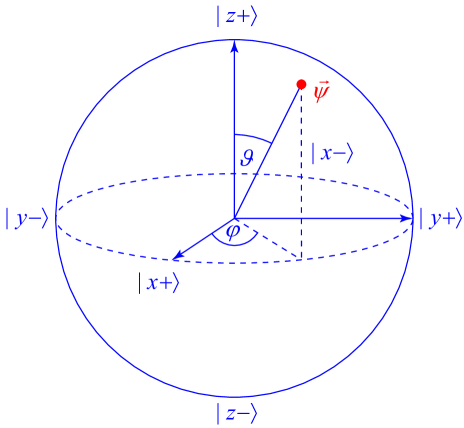
Figure 8: The Bloch sphere representation of a qubit. The quantum state is represented as a point $\vec{\psi}$ on the surface of a unit 2-sphere.

In the Kochen–Specker model, the ontic state space is the unit sphere $\Lambda=S_{2}$, which can be thought of as the Bloch sphere. The quantum state $\left[\psi\right]$ corresponds to a measure $\mu$ that can be written as

$$\mu(\Omega)=\int_{\Omega}p(\vec{\lambda})\sin\vartheta d\vartheta d\varphi,$$ (29)

where $\vec{\lambda}=(\sin\vartheta\cos\varphi,\sin\vartheta\sin\varphi,\cos\vartheta)$ and the density $p$ is given by

$$p(\vec{\lambda})=\frac{1}{\pi}H(\vec{\psi}\cdot\vec{\lambda})\vec{\psi}\cdot\vec{\lambda},$$ (30)

where $H$ is the Heaviside step function

$$H(x)=\begin{cases}1&\text{if}\,\,x>0\\ 0&\text{if}\,\,x\leq 0.\end{cases}$$ (31)

This density is nonzero on the hemisphere defined by all vectors that subtend an angle of less than $\pi/2$ with $\vec{\psi}$ and it takes values proportional to the cosine of the angle between $\vec{\lambda}$ and $\vec{\psi}$.

For a measurement $M=\left\{\left[\phi\right],\left[\phi^{\perp}\right]\right\}$, the outcome $\left[\phi\right]$ is obtained if the angle between $\vec{\lambda}$ and $\vec{\phi}$ is smaller than the angle between $\vec{\lambda}$ and $\vec{\phi^{\perp}}$. Otherwise the outcome $\left[\phi^{\perp}\right]$ is obtained. This corresponds to the conditional probabilities

$$\text{Pr}(\phi|M,\vec{\lambda}) =H(\vec{\phi}\cdot\vec{\lambda})$$ (32)

$$\text{Pr}(\phi^{\perp}|M,\lambda) =1-\text{Pr}(\phi|M,\vec{\lambda}).$$ (33)

A proof that this reproduces the quantum predictions is given in Appendix B.

4.4 Defining $\psi$-ontic/epistemic models

We are now in a position to formally define what it means for the quantum state to be real within an ontological model. The definition presented here is the one used by Pusey–Barrett–Rudolph [27], which is a slightly more rigorous version of a definition originally introduced by Harrigan and Spekkens [74]. It is uncontroversial that mixed states at least sometimes represent knowledge about which of a set of pure states was prepared, so they are at least partially epistemic. For this reason, $\psi$-ontology theorems are only concerned with proving the reality of pure quantum states. A $\psi$-ontic model is then one in which, if the pure state $\left[\psi\right]$ is prepared, then $\left[\psi\right]$ is part of the ontic state of the system. In other words, the ontic state space can be thought of as being composed of the set of pure quantum states along with possibly some extra hidden variables. This will be the case if the measures corresponding to distinct pure state preparations do not overlap with one another (see Fig. 9). Conversely, the $\psi$-epistemic explanations of quantum phenomena discussed in §2.1 depend crucially on having overlap between the measures representing different quantum states, so whether or not there is overlap is the key issue.

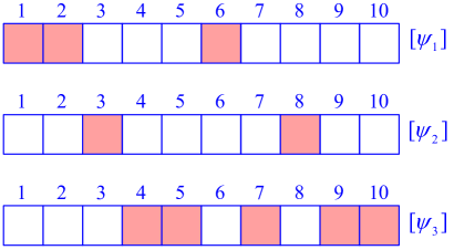
(a) Ontic model with nonoverlapping quantum states.

Old label New label $1$ $(\psi_{1},1)$ $2$ $(\psi_{1},2)$ $3$ $(\psi_{2},1)$ $4$ $(\psi_{3},1)$ $5$ $(\psi_{3},2)$ $6$ $(\psi_{1},3)$ $7$ $(\psi_{3},3)$ $8$ $(\psi_{2},2)$ $9$ $(\psi_{3},4)$ $10$ $(\psi_{3},5)$

(b) Relabeling the ontic states.

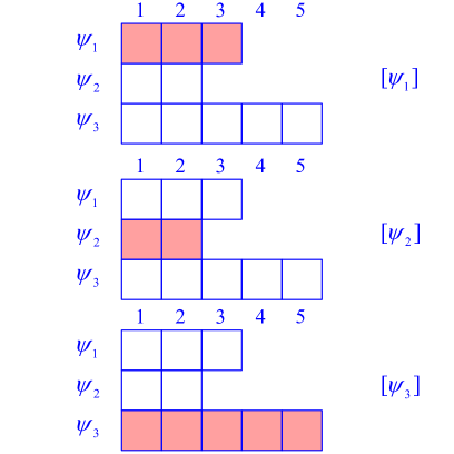
(c) Equivalent model in which the quantum state is explicitly part of the ontology.

Figure 9: In an ontological model, if the probability measures corresponding to distinct quantum states do not overlap, then the ontic states can be relabeled such that the quantum state is explicitly part of the ontology. Panel LABEL:sub@fig:POEM:relabel:start depicts the measures corresponding to three quantum states on a discrete ontic state space consisting of the integers from $1$ to $10$. Red boxes indicate the ontic states on which the measures have support. Panel LABEL:sub@fig:POEM:relabel:relabel shows a one-to-one map to a new ontic state space in which the quantum states are an explicit part of the ontology. The result is shown in Panel LABEL:sub@fig:POEM:relabel:end.

The notion of when two probability measures overlap can be formalized using the variational distance.

Definition 4.7.

The variational distance between two probability measures $\mu$ and $\nu$ on a measurable space $(\Lambda,\Sigma)$ is

$$D(\mu,\nu)=\sup_{\Omega\in\Sigma}\left|\mu(\Omega)-\nu(\Omega)\right|.$$ (34)

Note that taking the absolute value in Eq. (34) is optional, since if $\nu(\Omega)>\mu(\Omega)$ for some $\Omega\in\Sigma$ then

$$\mu(\Lambda\backslash\Omega)-\nu(\Lambda\backslash\Omega)=1-\mu(\Omega)-1+\nu(\Omega)=\nu(\Omega)-\mu(\Omega),$$ (35)

so there is always another measurable set for which the difference of the measures is the same, but $\mu$ is larger than $\nu$. Thus, the variational distance can equivalently be defined as

$$D(\mu,\nu)=\sup_{\Omega\in\Sigma}\left(\mu(\Omega)-\nu(\Omega)\right),$$ (36)

or indeed

$$D(\mu,\nu)=\sup_{\Omega\in\Sigma}\left(\nu(\Omega)-\mu(\Omega)\right).$$ (37)

The variational distance is a metric on the set of probability measures and it has the following operational interpretation. Suppose that a system is prepared according to one of two preparation procedures, $P_{1}$ or $P_{2}$, where $P_{1}$ corresponds to the measure $\mu$ and the $P_{2}$ to the measure $\nu$, each case having an equal a priori probability. You are then told the actual value of $\lambda$ and you wish to make the best possible guess as to which of the two preparation procedures was used. Your best strategy will be to choose a set $\Omega\subseteq\Lambda$ and guess $P_{1}$ if $\lambda\in\Omega$ and $P_{2}$ if $\lambda\notin\Omega$. More generally, you could use a probabilistic procedure, but convexity implies that this cannot increase your probability of success. Your probability of success is then

$$\text{Prob}(P_{1})\text{Prob}(\Omega|P_{1})+\text{Prob}(P_{2})\text{Prob}(\Lambda\backslash\Omega|P_{2})$$

$$=\frac{1}{2}\mu(\Omega)+\frac{1}{2}\nu(\Lambda\backslash\Omega)=\frac{1}{2}\left(1+\mu(\Omega)-\nu(\Omega)\right),$$ (38)

so the maximum probability of success over all such strategies is $\frac{1}{2}\left(1+D(\mu,\nu)\right)$. Success can occur with unit probability only when $D(\mu,\nu)=1$, so in this case $\lambda$ effectively determines which probability density was prepared uniquely.

More rigorously, $D(\mu,\nu)=1$ is equivalent to the existence of a measurable set $\Omega\in\Sigma$ such that $\mu(\Omega)=1$ and $\nu(\Omega)=0$. An optimal guessing strategy then consists of guessing $\mu$ if $\lambda\in\Omega$ and $\nu$ if $\lambda\notin\Omega$.

If $\mu$ and $\nu$ are dominated by a third measure $m$, i.e.

$$\mu(\Omega) =\int_{\Omega}p(\lambda)dm(\lambda)$$ (39)

$$\nu(\Omega) =\int_{\Omega}q(\lambda)dm(\lambda),$$ (40)

for some $m$-measurable densities $p$ and $q$, then

$$D(\mu,\nu)=\frac{1}{2}\int_{\Lambda}\left|p(\lambda)-q(\lambda)\right|dm(\lambda),$$ (41)

which is often the most convenient form for computation.

For those unfamiliar with measure-theoretic probability, a measure $m$ dominates a measure $\mu$ if, whenever $m(\Omega)=0$ then $\mu(\Omega)=0$. If this holds then $\mu$ can be written as a density with respect to $m$. The measure $m=\frac{1}{2}\left(\mu+\nu\right)$ dominates both $\mu$ and $\nu$, and a similarly for any finite set of probability measures. For an uncountable set of measures there need not exist a measure that dominates all of them. For example, there is no measure that dominates all of the point measures $\delta_{\psi}$ occurring in the Beltrametti–Bugajski model, which is one of the reasons why we work with probability measures instead of probability densities in the present treatment.

Based on the variational distance, we can define what it means for two quantum states to have no overlap in an ontic model.

Definition 4.8.

A pair of quantum states $\rho,\sigma\in\mathcal{P}$ are ontologically distinct in an ontological model if, for all $\mu\in\Delta_{\rho},\nu\in\Delta_{\sigma}$,

$$D(\mu,\nu)=1,$$ (42)

otherwise they are ontologically indistinct.

The idea here is that, if $\rho$ and $\sigma$ are ontologically distinct then, regardless of how they are prepared, they can be perfectly distinguished given knowledge of the exact ontic state. In order to take preparation contextuality into account, all possible pairs of preparations that are represented by $\rho$ and $\sigma$ must correspond to measures that have zero overlap.

If a set of preparations is operationally distinguishable, i.e. there exists a measurement that perfectly distinguishes them, then they must also be ontologically distinct. The intuition behind this is straightforward. Consider the case of a finite ontic state space. If the measures corresponding to two operationally distinguishable preparations did have nontrivial overlap then there would be a finite probability of an ontic state occurring that is assigned a finite probability according to both of them, and if this happens then the ontic state cannot be used to deduce which preparation was performed with certainty. Hence, such a model could not reproduce the statistics of the distinguishing measurement, which does allow this deduction. More formally,

Definition 4.9.

A finite set of quantum states $\left\{\rho_{j}\right\}\subseteq\mathcal{P}$ is operationally distinguishable if there exists a POVM $\{E_{j}\}\in\mathcal{M}$ such that

$$\text{Tr}\left(E_{j}\rho_{k}\right)=\delta_{jk}.$$ (43)

Theorem 4.10.

Let $\mathcal{D}\subseteq\mathcal{P}$ be an operationally distinguishable set of states. Then, every pair $\rho,\sigma\in\mathcal{D}$, $\rho\neq\sigma$, is ontologically distinct in any ontological model that reproduces the operational predictions.

Proof.

Let $M\in\mathcal{M}$ be a measurement that distinguishes the states in $\mathcal{D}$. Then, for $\rho,\sigma\in\mathcal{D}$, $\rho\neq\sigma$, there exists a POVM element $E\in M$ such that

$$\text{Tr}\left(E\rho\right)=1\qquad\text{and}\qquad\text{Tr}\left(E\sigma\right)=0.$$ (44)

In an ontological model that reproduces the quantum predictions, this implies that

$$\int_{\Lambda}\text{Pr}(E|M,\lambda)d\mu(\lambda) =1$$ (45)

$$\int_{\Lambda}\text{Pr}(E|M,\lambda)d\nu(\lambda) =0,$$ (46)

for all $\mu\in\Delta_{\rho}$, $\nu\in\Delta_{\sigma}$, and for any $\text{Pr}\in\Xi_{M}$.

Assume that $\rho$ and $\sigma$ are ontologically indistinct. Then, there exist $\mu\in\Delta_{\rho}$, $\nu\in\Delta_{\sigma}$ such that $D(\mu,\nu)<1$. This is equivalent to saying that all sets that are of measure $1$ according to $\mu$ are of nonzero measure according to to $\nu$. In order to satisfy Eq. (45), $\text{Pr}(E|M,\lambda)$ must be equal to $1$ on a set $\Omega$ that is of measure one according to $\mu$, and thus by ontological indistinctness $\nu(\Omega)>0$. However, from Eq. (46) we have

$$0 =\int_{\Lambda}\text{Pr}(E|M,\lambda)d\nu(\lambda)$$ (47)

$$\geq\int_{\Omega}\text{Pr}(E|M,\lambda)d\nu(\lambda)$$ (48)

$$=\int_{\Omega}d\nu(\lambda)=\nu(\Omega)>0,$$ (49)

which is a contradiction. ∎

Although operationally distinguishable quantum states are always ontologically distinct, this argument does not imply that arbitrary pairs of states are. If all pairs of pure states are nonetheless ontologically distinct then the ontological model is $\psi$-ontic.

Definition 4.11.

An ontological model is $\psi$-ontic if all pairs of pure quantum states $\left[\psi\right],\left[\phi\right]\in\mathcal{P}$, $\left[\psi\right]\neq\left[\phi\right]$, are ontologically distinct. Otherwise the model is $\psi$-epistemic.

This definition captures the idea that quantum states are real in an ontological model if the probability measures corresponding to distinct pure states do not overlap. Defining a $\psi$-epistemic model to be the negation of this is extremely permissive. For example, a model in which only a single pair of pure states have any overlap, all other pairs being ontologically distinct, would be $\psi$-epistemic according to this definition. The $\psi$-epistemic explanations of quantum phenomena discussed in §2.1 would not apply to such a model. The $\psi$-ontology theorems discussed in Part II aim to rule out even this permissive notion of a $\psi$-epistemic model, so they obviously rule out any less permissive definition as well. Nevertheless, because $\psi$-ontology theorems require questionable auxiliary assumptions, it is still interesting to consider stronger notions of what it means for the quantum state to be epistemic. This is done in in §5.2 and Part III.

Note that a $\psi$-ontic model is not necessarily $\psi$-complete, where the latter means that the wavefunction, and only the wavefunction, is the ontic state. $\psi$-complete models are obviously $\psi$-ontic, but in general $\psi$-ontic models may involve other variables in addition to the wavefunction. A lot of confusion may be avoided by clearly separating the notions of $\psi$-ontic and $\psi$-complete models, particularly since much of the literature on hidden variable theories focuses on the question of whether quantum theory is complete, i.e. it is assumed that the wavefunction is real a priori and the only question is whether anything else needs to be added to it. Obviously, such a framework is not suited to discussing the question of whether the wavefunction must be real in the first place.

Of the examples considered in §4.3, Spekkens’ toy theory and the Kochen–Specker model are $\psi$-epistemic, and the Beltrametti–Bugajski and Bell models are $\psi$-ontic. In Spekkens’ theory, the ontic state space is finite, so the integral in Eq. (41) can be performed with respect to the counting measure, which yields the sum

$$D(\mu,\nu)=\frac{1}{2}\sum_{\lambda}|\mu(\lambda)-\nu(\lambda)|.$$ (50)

For toy bit, $\lambda$ takes the values $(+,+),(+,-),(-,+)$ and $(-,-)$. If $\mu$ is the $\left|x+\right)$ measure, corresponding to the quantum state $\left[x+\right]$, and $\nu$ is $\left|y+\right)$, corresponding to $\left[y+\right]$ then we have

$$D(\mu,\nu)=\frac{1}{2}\left(\left|\frac{1}{2}-\frac{1}{2}\right|+\left|\frac{1}{2}-0\right|+\left|0-\frac{1}{2}\right|+\left|0-0\right|\right)=\frac{1}{2}.$$ (51)

Thus, the model is $\psi$-epistemic because $D(\mu,\nu)<1$, as we expect for overlapping measures. Appendix B provides a proof that the Kochen–Specker model is $\psi$-epistemic by showing that it satisfies the stronger notion of being maximally $\psi$-epistemic to be discussed in §5.2.

The Beltrametti–Bugajski model is in fact $\psi$-complete, because its ontic state space consists of the set of pure states and preparing a given pure state causes the corresponding ontic state to be occupied with certainty. It follows that the model is $\psi$-ontic because each pure state corresponds to a distinct point measure. Thus, for $\left[\psi\right]\neq\left[\phi\right]$ the corresponding measures are $\delta_{\psi}$ and $\delta_{\phi}$. The set $\left\{\left[\psi\right]\right\}$ is measure one according to $\delta_{\psi}$ and measure zero according to $\delta_{\phi}$. Similarly, the Bell model is $\psi$-ontic, where now the set $\left\{\left[\psi\right]\right\}\times[0,1]$ is measure one for the measure corresponding to $\left[\psi\right]$ and measure zero for the measure corresponding to $\left[\phi\right]$. It is, however, not $\psi$-complete because of the additional component $[0,1]$ of the ontic state space.

5 Implications of $\psi$-ontology

Before discussing $\psi$-ontology theorems, it is worth pausing to consider some of their implications. One of the most interesting things about establishing the reality of the quantum state within the ontological models framework is that it would imply a lot of existing no-go results as simple consequences. Thus, even if you are a neo-Copenhagenist who rejects the ontological models framework outright, you should still be interested in $\psi$-ontology theorems as potentially the most powerful class of no-go results that we currently have. Additionally, the ontological models framework can be thought of as an attempt to simulate quantum theory using classical resources. Just as Bell’s Theorem has implications for the difference between quantum and classical communication complexity, and for device independent quantum cryptography [102], $\psi$-ontology theorems might become a useful tool in quantum information theory.

The main implications of $\psi$-ontology are illustrated in Fig. 10, and each of them is discussed in this section. There are two main strands of implications, one based on the size of the ontic state space and one based on results related to contextuality. The results of the contextuality strand can alternatively be derived as consequences of the Kochen–Specker Theorem. Since $\psi$-ontology is our main concern here, the connection to the Kochen–Specker theorem is discussed in Appendix C.

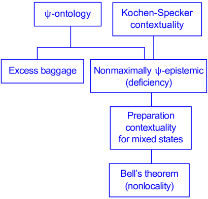
Figure 10: Hierarchy of constraints on ontological models of quantum theory. Properties that appear higher in the diagram imply those that they are connected to lower down. Non maximal $\psi$-epistemicity can be derived from either $\psi$-ontology or Kochen–Specker contextuality.

5.1 Excess baggage

The idea of excess baggage has already been discussed in §2.5 as the tension between the infinite amount of information required to specify the quantum state of a qubit and the fact that it can only be used to reliably transmit a single bit. Similarly, the number of parameters required to specify a quantum state scales exponentially with the number of systems, but the amount of information that can be transmitted scales only linearly.

Excess baggage theorems show that this tension cannot be avoided in an ontological model by providing lower bounds on the size of the ontic state space required to reproduce quantum theory. The first such result, from which the “excess baggage” terminology originates, was due to Hardy, who proved that an infinite number of ontic states are required to reproduce the predictions of any quantum system, even just a qubit [61]. Subsequently, Montina showed that the number of parameters required to specify an ontic state must scale exponentially with the number of systems [62, 63].

If it can be proved that an ontological model of quantum theory must be $\psi$-ontic then it follows immediately that the ontic state space must be uncountably infinite and that the number of parameters required to specify an ontic state must scale exponentially with the number of systems. This is because, in a $\psi$-ontic model, there must be at least as many ontic states as there are quantum states.

5.2 Maximally $\psi$-epistemic models

The concept of a maximally $\psi$-epistemic model was introduced by Maroney as a stronger notion of what it means for an ontological model to be $\psi$-epistemic [58]. An equivalent concept was introduced earlier by Harrigan and Rudolph [98], under the terminology “non deficient model”. As you might imagine from the name, a $\psi$-ontic model cannot be maximally $\psi$-epistemic, but, even without $\psi$-ontology, maximally $\psi$-epistemic models are ruled out by the Kochen–Specker theorem, as discussed in Appendix C.

The real interest in the concept of a maximally $\psi$-epistemic model is that it enables one to devise measures of the extent to which a model is $\psi$-epistemic, and hence to go beyond the sharp dichotomy between $\psi$-epistemic and $\psi$-ontic implied by the definitions adopted so far [58, 54, 57, 55]. This aspect is discussed in §12.2, but the concept of a maximally $\psi$-epistemic model is also useful as a stepping stone between $\psi$-ontology and the next step in the contextuality strand, which is preparation contextuality.

The basic idea is that, in order to justify the $\psi$-epistemic explanation of indistinguishability, we need more than just that the probability measures corresponding to two different quantum states, $\left[\psi\right]$ and $\left[\phi\right]$, should have nonzero overlap. Ideally, when measuring a system prepared in the state $\left[\psi\right]$, all of the probability of obtaining the outcome corresponding to the projector $\left[\phi\right]$ should be accounted for by the overlap region between the probability measures corresponding to the two states. Since we are comparing the overlap of $\left[\psi\right]$ and $\left[\phi\right]$, considered as states, with the probability of obtaining $\left[\phi\right]$ as a measurement outcome, this only makes sense if we are dealing with a PM fragment for which, for every pure state $\left[\phi\right]\in\mathcal{P}$, there exists a measurement $M\in\mathcal{M}$ such that $\left[\phi\right]\in\mathcal{M}$. Therefore, this is a standing assumption for the remainder of this section.

Definition 5.1.

An ontological model of a PM fragment is maximally $\psi$-epistemic if, for every pair of pure states $\left[\psi\right],\left[\phi\right]\in\mathcal{P}$, for all $\mu\in\Delta_{\psi}$, $\nu\in\Delta_{\phi}$, $M\in\mathcal{M}$ with $\left[\phi\right]\in M$, and $\text{Pr}\in\Xi_{M}$,

$$\int_{\Omega}\text{Pr}(\phi|M,\lambda)d\mu(\lambda)=\int_{\Lambda}\text{Pr}(\phi|M,\lambda)d\mu(\lambda),$$ (52)

for all sets $\Omega\in\Sigma$ such that $\nu(\Omega)=1$.

To unpack this definition a little, let $\mu\in\Delta_{\psi}$, let $\nu\in\Delta_{\phi}$, let $M$ be a measurement that contains $\left[\phi\right]$, and let $\text{Pr}\in\Xi_{M}$. Suppose $\Omega$ is a set of measure one according to $\nu$ and $\Omega^{\prime}$ is a set of measure one according to $\mu$. Then, Eq. (52) is equivalent to

$$\int_{\Omega\cap\Omega^{\prime}}\text{Pr}(\phi|M,\lambda)d\mu(\lambda)=\int_{\Lambda}\text{Pr}(\phi|M,\lambda)d\mu(\lambda).$$ (53)

Whatever one might mean by the overlap region between $\mu$ and $\nu$, it should be the intersection of a set that is measure one according to $\mu$ with a set that is measure one according to $\nu$, and since Eq. (53) must hold for all such sets, it guarantees that the probability of obtaining outcome $\left[\Phi\right]$ when measuring a system prepared in the state $\left[\psi\right]$ is entirely accounted for by any such region.

Note that, instead of Eq. (52), previous works [98, 58, 59, 56] imposed the requirement that

$$\int_{\Lambda_{q}}\text{Pr}(\phi|M,\lambda)p(\lambda)d\lambda=\int_{\Lambda}\text{Pr}(\phi|M,\lambda)p(\lambda)d\lambda,$$ (54)

where $d\lambda$ is a measure that dominates $\mu$ and $\nu$, $p$ and $q$ are densities that represent them, and $\Lambda_{q}=\{\lambda\in\Lambda|q(\lambda)>0\}$ is the support of the probability density $q$. However, the probability measure $\nu$ does not correspond to a unique density $q$, since densities that differ on a set of measure zero according to $d\lambda$ represent the same probability measure. This means that $\Lambda_{q}$ is not uniquely specified by $\nu$, since setting the values of $q$ to zero on a measure zero set would change $\Lambda_{q}$ but not $\nu$. Therefore, to use this definition, one has to imagine that the ontological model specifies a particular density representation for each measure, rather than just the measure itself. On its own, this older definition is also not strong enough to entail that a $\psi$-ontic model cannot be maximally $\psi$-epistemic. To remedy this, one can adopt a standing assumption that all probability measures appearing in the model are dominated by, i.e. absolutely continuous with respect to, a canonical measure $d\lambda$, as was done explicitly in [56], and this must be regarded as an implicit assumption in previous works [98, 58, 59]. However, we do not really want to make this assumption, because some models of interest do not satisfy it. For example, an uncountable set of point measures on distinct points is not dominated by any measure, and these occur in the Beltrametti–Bugajski and Bell models.

It is straightforward to verify that Spekkens’ toy theory is maximally $\psi$-epistemic and a proof that the Kochen–Specker model is maximally $\psi$-epistemic is given in Appendix B. On the other hand, a $\psi$-ontic model that reproduces the quantum predictions cannot be maximally $\psi$-epistemic, so the Beltrametti–Bugajski and Bell models are not maximally $\psi$-epistemic.

Theorem 5.2.

Consider a PM fragment that contains at least one pair of nonorthogonal pure states. If an ontological model of this fragment that reproduces the quantum predictions is maximally $\psi$-epistemic then it is $\psi$-epistemic.

Proof.

Assume the ontological model is $\psi$-ontic. Then, for every pair of nonorthogonal pure states $\left[\psi\right],\left[\phi\right]\in\mathcal{P}$, every pair $\mu\in\Delta_{\psi}$, $\nu\in\Delta_{\phi}$ satisfies $D(\mu,\nu)=1$, which is equivalent to saying that there exists a set $\Omega$ that is measure $0$ according to $\mu$ and measure $1$ according to $\nu$. However, if the ontological model is maximally $\psi$-epistemic then, for all $\mu\in\Delta_{\psi}$, $\nu\in\Delta_{\phi}$, $M\in\mathcal{M}$ containing $\left[\phi\right]$, and $\text{Pr}\in\Xi_{M}$,

$$\int_{\Omega}\text{Pr}(\phi|M,\lambda)d\mu(\lambda)=\int_{\Lambda}\text{Pr}(\phi|M,\lambda)d\mu(\lambda).$$ (55)

This implies that,

$$\mu(\Omega) =\int_{\Omega}d\mu(\lambda)$$ (56)

$$\geq\int_{\Omega}\text{Pr}(\phi|M,\lambda)d\mu(\lambda)$$ (57)

$$=\int_{\Lambda}\text{Pr}(\phi|M,\lambda)d\mu(\lambda)$$ (58)

$$=\text{Tr}\left(\left[\phi\right]\left[\psi\right]\right)>0,$$ (59)

where the second line follows from the fact that $\text{Pr}(\phi|M,\lambda)\in[0,1]$ and the fourth from the fact that the ontological model reproduces the quantum predictions. Thus, $\Omega$ cannot be of measure zero according to $\mu$, which contradicts the assertion that the model is $\psi$-ontic. ∎

5.3 Preparation contextuality

In [67], Spekkens introduced an operational approach to contextuality. In addition to generalizing the usual Kochen–Specker approach to contextuality of measurements, as discussed in Appendix C, Spekkens introduced a notion of contextuality for preparations. In Spekkens’ approach, the fundamental idea of noncontextuality is that things that are operationally equivalent, i.e. always lead to the same observable probabilities, should be represented in the same way in an ontological model. Preparation noncontextuality is just this idea applied to states rather than measurements. This section shows that, when extended to mixed states, non maximally $\psi$-epistemic models must be preparation contextual, a result that was first pointed out in [56].

Definition 5.3.

In an ontological model of a PM fragment, a state $\rho\in\mathcal{P}$ is preparation noncontextual if $\Delta_{\rho}$ only contains a single measure. Otherwise $\rho$ is preparation contextual. Similarly, the ontological model itself is preparation noncontextual if every $\rho\in\mathcal{P}$ is preparation noncontextual, and otherwise it is preparation contextual.

Whenever two preparation procedures result in the same quantum state $\rho$, there is no measurement that can distinguish between them because, according to quantum theory, all of the outcome probabilities for every measurement are exactly the same. Thus, the general principle of noncontextuality implies that all methods of preparing $\rho$ should result in the same probability measure.

Note that much of the literature on $\psi$-ontology implicitly assumes preparation noncontextuality for pure states by associating a unique measure $\mu_{\psi}$ with each pure state $\left[\psi\right]$ under consideration. This assumption is fairly harmless for a couple of reasons. Firstly, the necessity of preparation contextuality has so far only been established for mixed states, so assuming a unique measure for pure states is not ruled out by any existing no-go theorem. Secondly, adapting results to preparation contextual models is usually just a matter of modifying the definitions in a fairly obvious way that does not require proofs to be modified substantively. Nevertheless, I prefer to take the possibility of preparation contextuality into account explicitly because it is oddly asymmetric to allow for contextual measurements but not contextual states, and because it allows results to be proved under weaker assumptions.

In order to prove preparation contextuality for mixed states, a further assumption is required about how convex combinations of quantum states should be represented in ontological models. To understand this, let $\rho=\sum_{j}p_{j}\sigma_{j}$ be a convex decomposition of a mixed state $\rho$ into other (pure or mixed) states $\sigma_{j}$, i.e. $0\leq p_{j}\leq 1$ and $\sum_{j}p_{j}=1$. One method of preparing $\rho$ is to generate a classical random variable that takes value $j$ with probability $p_{j}$ (e.g. by flipping coins, throwing dice, or any other suitable method), prepare the state $\sigma_{j}$ if the value of the classical variable is $j$, and then discard and forget the value of the classical variable.

In an ontological model, it is reasonable to assume that, in the above mixing procedure, if $\mu_{j}$ is the probability measure corresponding to the method used to prepare $\sigma_{j}$, then $\sum_{j}p_{j}\mu_{j}$ is the measure corresponding to preparing $\rho$ by this mixing procedure. This is because the randomness used to generate the classical variable could come from a source that is completely independent of the system under investigation, in which case we would expect that the ontic state of the system only depends on it via its effect on which of the $\sigma_{j}$ is prepared. More formally,

Definition 5.4.

An ontological model respects convex decompositions of a state $\rho\in\mathcal{P}$ if, for every set of states $\{\sigma_{j}\}\subseteq\mathcal{P}$ such that $\rho=\sum_{j}p_{j}\sigma_{j}\in\mathcal{P}$ for some coefficients $p_{j}$ satisfying $0\leq p_{j}\leq 1$ and $\sum_{j}p_{j}=1$, for all possible choices of $\mu_{j}\in\Delta_{\sigma_{j}}$, the measure $\sum_{j}p_{j}\mu_{j}$ is in $\Delta_{\rho}$. The ontological model respects convexity if it respects convex decompositions of every $\rho\in\mathcal{P}$.

For the purpose of connecting non maximally $\psi$-epistemic models with preparation contextuality, recall that an ontological model is non maximally $\psi$-epistemic iff there are two nonorthogonal pure states $\left[\psi\right],\left[\phi\right]\in\mathcal{P}$, such that, for some $\mu\in\Delta_{\psi}$, $\nu\in\Delta_{\phi}$, $M\in\mathcal{M}$ containing $\left[\phi\right]$, and $\text{Pr}\in\Xi_{M}$ there exists an $\Omega\in\Sigma$ such that $\nu(\Omega)=1$ but

$$\int_{\Omega}\text{Pr}(\phi|M,\lambda)d\mu(\lambda)<\int_{\Lambda}\text{Pr}(\phi|M,\lambda)d\mu(\lambda).$$ (60)

Preparation contextuality can now be derived from non maximal $\psi$-epistemicity via the following theorem.

Theorem 5.5.

Consider an ontological model of a PM fragment that reproduces the quantum predictions, respects convexity and is non maximally $\psi$-epistemic.

Assume that, for some pair of pure states $\left[\psi\right],\left[\phi\right]\in\mathcal{P}$ that satisfy Eq. (60), the states $\sigma^{\psi^{\perp}}=\frac{1}{d-1}\left(I-\left[\psi\right]\right)$, $\sigma^{\phi^{\perp}}=\frac{1}{d-1}\left(I-\left[\phi\right]\right)$ and the maximally mixed state $I/d$ are also in $\mathcal{P}$. Then, $I/d$ is preparation contextual in the ontological model.

Proof.

The maximally mixed state has convex decompositions

$$\frac{I}{d} =\frac{1}{d}\left[\psi\right]+\frac{d-1}{d}\sigma^{\psi^{\perp}}$$ (61)

$$=\frac{1}{d}\left[\phi\right]+\frac{d-1}{d}\sigma^{\phi^{\perp}}.$$ (62)

Since the ontological and quantum models respect convexity, for every $\mu\in\Delta_{\psi}$ and $\mu^{\perp}\in\Delta_{\sigma^{\psi^{\perp}}}$, the measure $\frac{1}{d}\mu+\frac{d-1}{d}\mu^{\perp}$ is in $\Delta_{I/d}$. Similarly, for every $\nu\in\Delta_{\phi}$ and $\nu^{\perp}\in\Delta_{\sigma^{\phi^{\perp}}}$, the measure $\frac{1}{d}\nu+\frac{d-1}{d}\nu^{\perp}$ is in $\Delta_{I/d}$. Assume that $I/d$ is preparation noncontextual, so that $\Delta_{I/d}$ only contains one probability measure $\zeta$. Then, we have

$$\zeta =\frac{1}{d}\mu+\frac{d-1}{d}\mu^{\perp}$$ (63)

$$=\frac{1}{d}\nu+\frac{d-1}{d}\nu^{\perp}.$$ (64)

Now, since $\left[\psi\right]$ and $\left[\phi\right]$ satisfy Eq. (60), and the model reproduces the quantum predictions, there must exist a $\mu\in\Delta_{\psi}$, a $\nu\in\Delta_{\phi}$, an $M\in\mathcal{M}$ containing $\left[\phi\right]$, a $\text{Pr}\in\Xi_{M}$, and a set $\Omega\in\Sigma$ such that $\nu(\Omega)=1$, but

$$\int_{\Omega}\text{Pr}(\phi|M,\lambda)d\mu(\lambda)<\text{Tr}\left(\left[\phi\right]\left[\psi\right]\right).$$ (65)

This means that, in order to reproduce the quantum predictions, there must be a set $\tilde{\Omega}\subseteq\Lambda\backslash\Omega$ such that $\text{Pr}(\phi|M,\lambda)$ is nonzero everywhere on $\tilde{\Omega}$ and $\mu(\tilde{\Omega})>0$. It is also the case that $\nu(\tilde{\Omega})=0$ because $\tilde{\Omega}$ is a subset of $\Lambda\backslash\Omega$ and $\Omega$ is measure one for $\nu$.

Again, since the ontological model reproduces the quantum predictions, we must have

$$\int_{\Omega}\text{Pr}(\phi|M,\lambda)d\nu^{\perp}(\lambda)=\text{Tr}\left(\left[\phi\right]\sigma^{\phi^{\perp}}\right)=0.$$ (66)

This implies that $\nu^{\perp}(\tilde{\Omega})=0$ because $\text{Pr}(\phi|M,\lambda)$ is nonzero everywhere on $\tilde{\Omega}$. Therefore we have

$$\zeta(\tilde{\Omega}) =\frac{1}{d}\nu(\tilde{\Omega})+\frac{d-1}{d}\nu^{\perp}(\tilde{\Omega})$$ (67)

$$=0,$$ (68)

but also

$$\zeta(\tilde{\Omega}) =\frac{1}{d}\mu(\tilde{\Omega})+\frac{d-1}{d}\mu^{\perp}(\tilde{\Omega})$$ (69)

$$\geq\frac{1}{d}\mu(\tilde{\Omega})$$ (70)

$$>0,$$ (71)

which is a contradiction. Therefore, $I/d$ must be preparation contextual. ∎

Similar arguments can be used to establish the preparation contextuality of other mixed states. If $\sigma$ and $\tau$ are states such that $\text{Tr}\left(\left[\phi\right]\sigma\right)=0$ and

$$p\left[\psi\right]+(1-p)\tau=q\left[\phi\right]+(1-q)\sigma,$$ (72)

for some $0\leq p,q\leq 1$, then the state $\rho=p\left[\psi\right]+(1-p)\tau$ must be preparation contextual by the same argument given above. Banik et. al. have recently used this method to show that all mixed states must be preparation contextual in Hilbert spaces of dimension $d\geq 3$ [103]. They also proved the same result for all Hilbert space dimensions, but via a method that does not make use of the connection with maximal $\psi$-epistemicity.

5.4 Bell’s Theorem

The purpose of this section is to argue that being committed to $\psi$-ontology implies the conclusion of Bell’s theorem, i.e. any $\psi$-ontic model must fail to satisfy Bell’s locality condition. It is not my intention to argue that the implication from $\psi$-ontology theorems to Bell’s theorem is the best or most elegant way of proving Bell’s theorem. The argument is quite technical compared to other proofs of Bell’s theorem and $\psi$-ontology theorems are based on auxiliary assumptions that are not required to prove Bell’s theorem. Instead, the aim is to compare the relative strength of the conclusions of $\psi$-ontology theorems with those of Bell’s theorem.

What we will actually do in this section is to argue that the kind of preparation contextuality that follows from the failure of maximal $\psi$-epistemicity implies the conclusion of Bell’s theorem. This means that $\psi$-ontology implies the same, because it can be used to establish the failure of maximal $\psi$-epistemicity. In principle, one can also view the result of this section as a full-blown proof of Bell’s theorem that does not rely on $\psi$-ontology, since, as established in Appendix C, the Kochen–Specker theorem can alternatively be used to establish the failure of maximal $\psi$-epistemicity without assuming the reality of the quantum state. However, this would be quite a convoluted way of deriving Bell’s theorem compared to the standard proofs.

From a historical perspective, the Einstein-Podolsky-Rosen argument [104] could be read as an argument that $\psi$-complete models are nonlocal, but a $\psi$-ontic model may involve other variables in addition to the wavefunction. That nonlocality follows from the weaker assumption of $\psi$-ontology is implicit in an argument that Einstein made in correspondence with Schrödinger. This was first pointed out by Harrigan and Spekkens in [74], where they also provide a more formal version of the argument. However, both the Einstein and Harrigan-Spekkens arguments employ an additional assumption known as Einstein separability, which is discussed in more detail in §7.3. Einstein separability is not actually required to prove Bell’s theorem [105], so I do not make this assumption here. This, in addition to taking care of measure-theoretic issues, makes the argument presented here a bit more involved than Harrigan and Spekkens’ treatment. However, once this is done, weakening their assumption of $\psi$-ontology to the failure of maximal $\psi$-epistemicity does not significantly change the structure of the argument. As presented here, the argument is based on an idea due to Barrett [106] that has appeared in the literature in an informal version [56].

The basic idea runs as follows. Suppose Alice and Bob share a composite system with Hilbert space $\mathcal{H}_{A}\otimes\mathcal{H}_{B}$, $\mathcal{H}_{A}=\mathcal{H}_{B}=\mathbb{C}^{d}$, prepared in the entangled state $\left[\Phi^{+}\right]_{AB}$, where

$$\left|\Phi^{+}\right\rangle_{AB}=\frac{1}{\sqrt{d}}\sum_{j=0}^{d-1}\left|j\right\rangle_{A}\otimes\left|j\right\rangle_{B},$$ (73)

and $\left\{\left|j\right\rangle\right\}_{j=0}^{d-1}$ is an orthonormal basis for $\mathbb{C}^{d}$. If Alice performs a measurement described by the projectors $\left\{\left[\psi\right]_{A}^{T},I_{A}-\left[\psi\right]_{A}^{T}\right\}$, where ^T denotes transpose in the $\left|j\right\rangle$ basis and $I_{A}$ is the identity operator on $\mathcal{H}_{A}$, then, with probability $1/d$ she obtains the $\left[\psi\right]_{A}^{T}$ outcome and the state of Bob’s system gets updated to $\left[\psi\right]_{B}$, and with probability $(d-1)/d$ she gets the $I_{A}-\left[\psi\right]_{A}^{T}$ outcome and the state of Bob’s system gets updated to $\sigma^{\psi{\perp}}_{B}$. If we allow Alice to postselect on her measurement outcome, then we can regard this as a method of preparing Bob’s system in the states $\left[\psi\right]_{B}$ and $\sigma^{\psi^{\perp}}_{B}$. If she subsequently forgets and discards her measurement outcome then we can also regard this as a method of preparing Bob’s system in the maximally mixed state by mixing $\left[\psi\right]_{B}$ with $\sigma^{\psi^{\perp}}_{B}$. Similar remarks apply if Alice measures $\{\left[\phi\right]^{T}_{A},I_{A}-\left[\phi\right]^{T}_{A}\}$, which, by postselection, prepares Bob’s system in the state $\left[\phi\right]_{B}$ or $\sigma^{\phi^{\perp}}_{B}$ and, upon forgetting the measurement outcome, prepares it in the maximally mixed state by mixing $\left[\phi\right]_{B}$ with $\sigma^{\phi^{\perp}}_{B}$.

Now, given an ontological model for the composite system that satisfies Bell’s locality condition, we can use it to derive an ontological model for these preparation procedures on Bob’s system alone. This model must be preparation noncontextual for the state $I/d$ because locality implies that the probability of getting a particular ontic state for the derived model on Bob’s system cannot depend on whether Alice chooses to measure $\left\{\left[\psi\right]^{T}_{A},I_{A}-\left[\psi\right]^{T}_{A}\right\}$ or $\left\{\left[\phi\right]^{T}_{A},I_{A}-\left[\phi\right]^{T}_{A}\right\}$. However, in order to construct a model for all possible preparations and measurements of this form that reproduces the quantum predictions, preparation noncontextuality must fail for some such pair because a maximally $\psi$-epistemic model is impossible. Therefore, Bell’s locality condition must fail. The remainder of this section formalizes this argument.

The type of PM fragment relevant to Bell’s Theorem involves a bipartite system and local measurements. This is formalized in the concept of a product measurement fragment.

Definition 5.6.

A product measurement fragment $\mathfrak{F}_{AB}=\langle\mathcal{H}_{A}\otimes\mathcal{H}_{B},\mathcal{P}_{AB},\mathcal{M}_{A}\times\mathcal{M}_{B}\rangle$ is a PM fragment on a composite system with Hilbert space $\mathcal{H}_{A}\otimes\mathcal{H}_{B}$, where $\mathcal{M}_{A}$ is a set of POVMs on $\mathcal{H}_{A}$, $\mathcal{M}_{B}$ is a set of POVMs on $\mathcal{H}_{B}$ and $\mathcal{M}_{A}\times\mathcal{M}_{B}$ denotes the set of all POVMs of the form $(M_{A},M_{B})=\{E_{j}\otimes F_{k}\}$, where $M_{A}=\{E_{j}\}\in\mathcal{M}_{A}$ and $M_{B}=\{F_{k}\}\in\mathcal{M}_{B}$.

To prove Bell’s Theorem, we only need consider a single bipartite state $\rho_{AB}$, so for the remainder of this section we assume that $\mathcal{P}_{AB}$ just contains this single state. Most of the concepts can be generalized to fragments with more than one state in an obvious way.

The first step is to reinterpret experiments on the composite system as prepare-and-measure experiments on Bob’s system alone. At the operational level, when the system is prepared in the state $\rho_{AB}$, Alice makes a measurement $M_{A}$ on system $A$ and Bob makes a measurement $M_{B}$ on system $B$, quantum theory predicts the outcome probabilities

$$\text{Prob}(E,F|M_{A},M_{B})=\text{Tr}_{AB}\left(E\otimes F\rho_{AB}\right),$$ (74)

where $E\in M_{A}$ and $F\in M_{B}$.

These probabilities can be rewritten in terms of states and measurements on $\mathcal{H}_{B}$ alone by imagining that Alice performs her measurement before Bob performs his, and considering how the state of Bob’s system gets updated in light of Alice’s measurement result. Upon learning that the outcome of $M_{A}$ was $E$, the state of Bob’s system gets updated to

$$\rho_{B|E}=\frac{\text{Tr}_{A}\left(E\otimes I_{B}\rho_{AB}\right)}{\text{Prob}(E|M_{A})},$$ (75)

where $\text{Prob}(E|M_{A})=\text{Tr}_{A}\left(E\rho_{A}\right)$ is the probability of Alice’s measurement outcome and $\rho_{A}=\text{Tr}_{B}\left(\rho_{AB}\right)$. Eq. (74) can then be rewritten as

$$\text{Prob}(E,F|M_{A},M_{B})=\text{Prob}(E|M_{A})\text{Tr}_{B}\left(F\rho_{B|E}\right).$$ (76)

By postselecting on obtaining the outcome $E$, Alice’s measurement can be viewed as a method of preparing Bob’s system in the state $\rho_{B|E}$. In doing so, $E$ gets reinterpreted as specifying a preparation procedure for system $B$, instead of a measurement on $A$, so we now want to condition the probabilities on $E$. This gives

$$\text{Prob}(F|M_{A},E,M_{B})=\frac{\text{Prob}(E,F|M_{A},M_{B})}{\text{Prob}(E|M_{A})}=\text{Tr}_{B}\left(F\rho_{B|E}\right).$$ (77)

We also want to consider the case where Alice forgets her measurement outcome outcome. This prepares Bob’s system in the state $\rho_{B}=\text{Tr}_{A}\left(\rho_{AB}\right)$ and we have, for every $M_{A}\in\mathcal{M}_{A}$,

$$\rho_{B}=\sum_{E\in M_{A}}\text{Prob}(E|M_{A})\rho_{B|E}.$$ (78)

We can now define the conditional fragment on Bob’s system consisting of all the states that Alice can prepare on his system in this way.

Definition 5.7.

Let $\mathfrak{F}_{AB}=\langle\mathcal{H}_{A}\otimes\mathcal{H}_{B},\mathcal{P}_{AB},\mathcal{M}_{A}\times\mathcal{M}_{B}\rangle$ be a product measurement fragment, where $\mathcal{P}_{AB}$ contains a single state $\rho_{AB}$. The conditional fragment on $B$ given $A$ is $\mathfrak{F}_{B|A}=\langle\mathcal{H}_{B},\mathcal{P}_{B|A},\mathcal{M}_{B}\rangle$, where $\mathcal{P}_{B|A}$ consists of all states of the form $\rho_{B|E}$ as given by Eq. (75) where $E\in M_{A}$ for some $M_{A}\in\mathcal{M}_{A}$, as well as the state $\rho_{B}=\text{Tr}_{A}\left(\rho_{AB}\right)$.

Typically, there are several different methods of preparing the same quantum state and of implementing the same measurement in a PM fragment. These different methods need not correspond to the same probability measures nor the same conditional probability distributions in an ontological model. However, the derivation of Bell’s theorem is greatly simplified if we focus attention on one specific method of preparing $\rho_{AB}$ and one one method of implementing each of the measurements $M_{A}\in\mathcal{M}_{A}$ and $M_{B}\in\mathcal{M}_{B}$. Then, we can assume that $\rho_{AB}$ is represented by a unique measure $\mu$ and that each $(M_{A},M_{B})$ is represented by a unique conditional probability distribution $\text{Pr}(E,F|M_{A},M_{B},\lambda)$, where $E\in M_{A}$ and $F\in M_{B}$. This does not weaken the conclusion because the result will hold regardless of which method of implementation is chosen. Therefore, for the remainder of this section, we assume a unique measure and conditional probabilities for ontological models of the product measurement fragment.

Given such an ontological model of $\mathfrak{F}_{AB}$, it is natural to think that an ontological model for the conditional PM fragment $\mathfrak{F}_{B|A}$ might be derivable from it. However, in general, an ontological model for $\mathfrak{F}_{AB}$ cannot be cleanly separated into a part that depends on system $A$ and a part that depends on system $B$ unless it satisfies Bell’s condition of local causality. To see this, suppose we have an ontological model of $\mathfrak{F}_{AB}$. If Alice chooses to make the measurement $M_{A}$ and Bob chooses to make the measurement $M_{B}$ then in general, not assuming locality, this is represented by a conditional probability distribution $\text{Pr}(E,F|M_{A},M_{B},\lambda)$, where $E\in M_{A}$ and $F\in M_{B}$. The model then predicts that the observed probability of obtaining the outcomes $E$ and $F$ is given by

$$\text{Pr}(E,F|M_{A},M_{B})=\int_{\Lambda}\text{Pr}(E,F|M_{A},M_{B},\lambda)d\mu(\lambda),$$ (79)

where $\mu$ is the measure representing $\rho_{AB}$.

At the quantum level, the conditional probability $\text{Prob}(F|M_{A},E,M_{B})$ could be rewritten in terms of a state on $\mathcal{H}_{B}$ that depends on $E$ alone and the measurement operator $F$, which is also defined on $\mathcal{H}_{B}$. The analogue at the ontological level would be to absorb the dependence on $M_{A}$ and $E$ into the measure $\mu$ and be left with a conditional probability distribution that only depends on $M_{B}$ and $F$. Unfortunately, the conditional probability distribution $\text{Pr}(E,F|M_{A},M_{B},\lambda)$ need not factor cleanly into a term that only depends on $E$ and $M_{A}$ and a term that only depends on $F$ and $M_{B}$. In order to obtain such a decomposition, a locality assumption is required.

Definition 5.8.

An ontological model of a product measurement fragment $\mathfrak{F}_{AB}=\langle\mathcal{H}_{A}\otimes\mathcal{H}_{B},\mathcal{P}_{AB},\mathcal{M}_{A}\times\mathcal{M}_{B}\rangle$ is Bell local if, for all $M_{A}\in\mathcal{M}_{A}$, $M_{B}\in\mathcal{M}_{B}$, $E\in M_{A}$, $F\in M_{B}$, $\lambda\in\Lambda$,

$$\text{Pr}(E,F|M_{A},M_{B},\lambda)=\text{Pr}(E|M_{A},\lambda)\text{Pr}(F|M_{B},\lambda)$$ (80)

where $\text{Pr}(E|M_{A},\lambda)$ is a valid conditional probability distribution over $M_{A}$ and $\text{Pr}(F|M_{B},\lambda)$ is a valid conditional probability distribution over $M_{B}$.

In a Bell local model of $\mathfrak{F}_{AB}$, measures conditional on $M_{A}$ and $E\in M_{A}$ can be defined as follows,

$$\mu_{M_{A},E}(\Omega)=\frac{1}{\text{Pr}(E|M_{A})}\int_{\Omega}\text{Pr}(E|M_{A},\lambda)d\mu(\lambda),$$ (81)

where $\text{Pr}(E|M_{A})=\int_{\Lambda}\text{Pr}(E|M_{A},\lambda)d\mu(\lambda)$ is the observed probability of obtaining the outcome $E$ for the measurement $M_{A}$ according to the ontological model. Eq. (80) can then be rewritten as

$$\text{Pr}(E,F|M_{A},M_{B},)=\text{Pr}(E|M_{A})\int_{\Lambda}\text{Pr}(F|M_{B},\lambda)d\mu_{M_{A},E}(\lambda),$$ (82)

and conditioning on $E$ gives

$$\text{Pr}(F|M_{A},E,M_{B})=\int_{\Lambda}\text{Pr}(F|M_{B},\lambda)d\mu_{M_{A},E}(\lambda),$$ (83)

which is the analogue of Eq. (77) at the ontological level.

Further, in the case where Alice does not report her measurement result we have,

$$\text{Pr}(F|M_{A},M_{B})=\int_{\Lambda}\text{Pr}(F|M_{B},\lambda)d\mu(\lambda),$$ (84)

Thus, an ontological model for the conditional theory can be defined as follows.

Definition 5.9.

Let $\mathfrak{F}_{AB}=\langle\mathcal{H}_{A}\otimes\mathcal{H}_{B},\mathcal{P}_{AB},\mathcal{M}_{A}\times\mathcal{M}_{B}\rangle$ be a product measurement fragment, where $\mathcal{P}_{AB}$ contains a single state $\rho_{AB}$, and consider a Bell local ontological model of it in which $\rho_{AB}$ is represented by a unique measure $\mu$, each $M_{A}\in\mathcal{M}_{A}$ is represented by a unique conditional probability distribution $\text{Pr}(E|M_{A},\lambda)$, and each $M_{B}\in\mathcal{M}_{B}$ is represented by a unique conditional probability distribution $\text{Pr}(F|M_{B},\lambda)$. Then, the conditional ontological model of the conditional fragment $\mathfrak{F}_{B|A}$ is defined by

• Placing the measure $\mu_{M_{A},E}$ in $\Delta_{\rho_{B|E}}$, where

  $$\mu_{M_{A},E}(\Omega)=\frac{1}{\text{Pr}_{A}(E|M_{A})}\int_{\Omega}\text{Pr}(E|M_{A},\lambda)d\mu(\lambda).$$ (85)

  Note that there may be more than one measure in $\Delta_{\rho_{B|E}}$ if $E$ occurs in more than one of the POVMs in $\mathcal{M}_{A}$.

• Associating the unique measure $\mu$ with the state $\rho_{B}=\text{Tr}_{A}\left(\rho_{AB}\right)$.

• Associating the unique conditional probability distribution $\text{Pr}(F|M_{B},\lambda)$ as defined in the Bell local model with each $M_{B}\in\mathcal{M}_{B}$.

It is straightforward to see that if the original ontological model reproduces the quantum predictions for $\mathfrak{F}_{AB}$ then the conditional ontological model reproduces the quantum predictions of $\mathfrak{F}_{B|A}$.

We now specialize to the product measurement fragment of interest for Bell’s Theorem. This is $\mathfrak{F}_{AB}=\left\langle\mathcal{H}_{A}\otimes\mathcal{H}_{B},\mathcal{P}_{AB},\mathcal{M}_{A}\times\mathcal{M}_{B}\right\rangle$, where $\mathcal{H}_{A}=\mathcal{H}_{B}=\mathbb{C}^{d}$, $\mathcal{P}_{AB}=\left\{\left[\Phi^{+}\right]_{AB}\right\}$, $\mathcal{M}_{A}$ consists of all projective measurements of the form $M_{A}=\{E_{0},E_{1}\}$ where $E_{0}=\left[\psi\right]$, $E_{1}=I_{A}-\left[\psi\right]$ for some $\left|\psi\right\rangle\in\mathbb{C}^{d}$ and $\mathcal{M}_{B}$ consists of all measurements on $\mathcal{H}_{B}$.

Given the available measurements in $\mathcal{M}_{A}$, $\rho_{B|E_{0}}$ is always a pure state and in fact Alice can prepare Bob’s system in any pure state by choosing an appropriate $E_{0}$, i.e. $\left[\psi\right]^{T}_{A}$ if she wants to prepare $\left[\psi\right]_{B}$.

Theorem 5.10.

Consider a Bell local model for the product measurement fragment $\mathfrak{F}_{AB}$ defined above that reproduces the quantum predictions for Alice’s measurements, i.e. for all $M_{A}\in\mathcal{M}_{A}$, $E\in M_{A}$,

$$\int_{\Lambda}\mathrm{Pr}(E|M_{A},\lambda)d\mu(\lambda)=\mathrm{Tr}_{AB}\left(E\otimes I_{B}\left[\Phi^{+}\right]_{AB}\right).$$ (86)

Then, the conditional ontological model of the conditional fragment $\mathfrak{F}_{B|A}$ is preparation noncontextual and respects convex decompositions.

Proof.

Given the choice of $\left[\Phi^{+}\right]_{AB}$, there is only one POVM $M_{A}=\{E_{0},E_{1}\}$ that can lead to a given conditional state $\rho_{B|E_{j}}$. The possible conditional states on Bob’s side are $\rho_{B|E_{0}}=\left[\psi\right]_{B}$ and $\rho_{B|E_{1}}=\sigma^{\psi^{\perp}}_{B}=\frac{1}{d-1}(I_{B}-\left[\psi\right]_{B})$, which occur when Alice makes the measurement $\{\left[\psi\right]^{T}_{A},I_{A}-\left[\psi\right]^{T}_{A}\}$, and so each of Alice’s measurements determine a unique pair of conditional states for Bob. Therefore, each $\Delta_{\rho_{B|E_{j}}}$ contains only a single measure, so the model is preparation noncontextual for these states. Similarly, by construction, there is a unique measure associated with $I/d$.

The only convex combinations that appear in $\mathfrak{F}_{B|A}$ are those of the form

$$\frac{I_{B}}{d}=\sum_{j=0}^{1}\text{Prob}(E_{j}|M_{A})\rho_{B|E_{j}},$$ (87)

where $\text{Prob}(E_{j}|M_{A})=\text{Tr}_{AB}\left(E_{j}\otimes I_{B}\left[\Phi^{+}\right]_{AB}\right)$. Therefore, the result follows if

$$\mu=\sum_{j=0}^{1}\text{Prob}(E_{j}|M_{A})\mu_{M_{A},E_{j}}.$$ (88)

To see this, note that $\sum_{j}\text{Pr}(E_{j}|M_{A},\lambda)=1$ for all $\lambda$, so, for $\Omega\in\Sigma$,

$$\mu(\Omega) =\int_{\Omega}d\mu(\lambda)$$ (89)

$$=\int_{\Omega}\left[\sum_{j}\text{Pr}(E_{j}|M_{A},\lambda)\right]d\mu(\lambda)$$ (90)

$$=\sum_{j}\int_{\Omega}\text{Pr}(E_{j}|M_{A},\lambda)d\mu(\lambda)$$ (91)

$$=\sum_{j}\text{Pr}(E_{j}|M_{A})\frac{1}{\text{Pr}(E_{j}|M_{A})}\int_{\Omega}\text{Pr}(E_{j}|M_{A},\lambda)d\mu(\lambda)$$ (92)

$$=\sum_{j}\text{Pr}(E_{j}|M_{A})\mu_{M_{A},E_{j}}(\Omega),$$ (93)

where $\text{Pr}(E_{j}|M_{A})=\int_{\Lambda}\text{Pr}(E_{j}|M_{A},\lambda)d\mu(\lambda)$ is the probability of Alice obtaining outcome $E_{j}$ when measuring $M_{A}$ according to the ontological model. By assumption, the model reproduces the quantum predictions for Alice’s measurements, so $\text{Pr}(E_{j}|M_{A})=\text{Prob}(E_{j}|M_{A})$, from which the result follows. ∎

Theorem 5.10 is enough to show that a $\psi$-ontic model of the above product measurement fragment that reproduces the quantum predictions cannot be Bell local. To see this note that Theorem 5.2 shows that a $\psi$-ontic model cannot be maximally $\psi$-epistemic and hence, by Theorem 5.5, if convexity is respected then preparation noncontextuality must fail for the maximally mixed state. However, a Bell local model would give rise to a preparation noncontextual ontological model for the conditional theory that respects convexity. Since the conditional fragment contains the states needed for Theorem 5.5, this implies that Bell locality must fail.

Note that, instead of relying on $\psi$-ontology one could use the Kochen–Specker theorem to rule out maximally $\psi$-epistemic theories for $d\geq 3$, as described in Appendix C. Then, Theorem 5.10 can be viewed as a full proof of Bell’s theorem that does not assume $\psi$-ontology, although this is quite complicated compared to the standard proofs.

Part II. $\psi$-ontology theorems

Having understood the implications of $\psi$-ontology, it is finally time to look at the extent to which it can be established. The first $\psi$-ontology theorem that was discovered is due to Pusey, Barrett and Rudolph. Of the available results, it is the most widely discussed in the literature and I think it makes the strongest case for $\psi$-ontology, so it receives the longest treatment in §7, including a discussion of generalizations and criticisms. Following this, I discuss two further $\psi$-ontology theorems: Hardy’s Theorem in §9, and the Colbeck–Renner Theorem in §10.

Before getting to these theorems, I discuss the concept of antidistinguishability in §6 because it plays a key role in both the Pusey–Barrett–Rudolph and Hardy’s theorems, as well as in some of the results discussed in Part III. Both Hardy’s Theorem and the Colbeck–Renner Theorem involve assumptions about how dynamics are represented in ontological models, so this is discussed in §8 after the discussion of Pusey–Barrett–Rudolph is completed.

6 Antidistinguishability

According to Theorem 4.10, sets of operationally distinguishable states are pairwise ontologically distinct in an ontological model. However, $\psi$-ontology requires that all pairs of pure states must be ontologically distinct, and most pairs of pure states are not orthogonal. Therefore, to prove $\psi$-ontology, it is useful to consider a weaker concept.

Definition 6.1.

A finite set of quantum states $\{\rho_{j}\}_{j=1}^{n}\subseteq\mathcal{P}$ is antidistinguishable if there exists a POVM $M=\left\{E_{j}\right\}_{j=1}^{n}\in\mathcal{M}$ such that, for each $j$,

$$\text{Tr}\left(E_{j}\rho_{j}\right)=0.$$ (94)

Recall that the definition of distinguishability states that there should exist a POVM $M=\{E_{j}\}_{j=1}^{n}\in\mathcal{M}$ such that $\text{Tr}\left(E_{k}\rho_{j}\right)=\delta_{jk}$ for all $j$ and $k$. This is equivalent to requiring $\text{Tr}\left(E_{j}\rho_{j}\right)=1$ for all $j$ by the following argument. Firstly, $\text{Tr}\left(E_{j}\rho_{j}\right)=1$ is obviously a special case of $\text{Tr}\left(E_{k}\rho_{j}\right)=\delta_{jk}$. For the converse direction note that if there were a $k\neq j$ such that $\text{Tr}\left(E_{k}\rho_{j}\right)>0$ then $\text{Tr}\left(\left(E_{j}+E_{k}\right)\rho_{j}\right)>1$, but this cannot be the case if $\rho_{j}$ is a density operator and $\{E_{j}\}_{j=1}^{n}$ is a POVM because then we must have $1=\text{Tr}\left(\rho_{j}\right)=\text{Tr}\left(\sum_{m}E_{m}\rho_{j}\right)\geq\text{Tr}\left(\left(E_{j}+E_{k}\right)\rho_{j}\right)$. Therefore, the difference between distinguishability and antidistinguishability is simply the replacement of $\text{Tr}\left(E_{j}\rho_{j}\right)=1$ with $\text{Tr}\left(E_{j}\rho_{j}\right)=0$. To understand what this means, suppose that one of the states in a set $\mathcal{D}$ is prepared and you do not know which. If $\mathcal{D}$ is distinguishable then there is a measurement for which each outcome identifies that a specific member of $\mathcal{D}$ was definitely the state prepared. On the other hand, if $\mathcal{D}$ is antidistinguishable then there is a measurement for which each outcome identifies that a specific member of $\mathcal{D}$ was definitely not the state prepared. In this sense, the two concepts are opposites.

Antidistinguishability is a weaker property than distinguishability because, if the measurement outcome $j$ tells us that $\rho_{j}$ was definitely prepared, then it also tells us that $\rho_{k}$ was definitely not prepared for all $k\neq j$. Therefore, a distinguishing measurement can be converted to an antidistinguishing one just by permuting the outcome indices in such a way that none of them are left invariant, e.g. if there are $n$ POVM elements then this can be done by mapping $j\rightarrow j+1$, where $n+1$ is identified with $1$. For sets of three or more states, antidistinguishability is strictly weaker than distinguishability, as there exist sets of nonorthogonal quantum states that can be antidistinguished (see Fig. 11 for an example). For a set of two states, antidistinguishability is equivalent to distinguishability because if you know that one of the states was not the one prepared then you know that it must have been the other one.

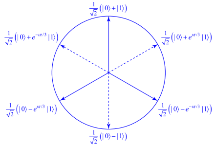
Figure 11: A set of nonorthogonal states that can be antidistinguished, and the POVM that antidistinguishes them. The diagram represents the equator of the Bloch sphere and the three antidistinguishable states are shown by the solid arrows. The dashed arrows show three states that are each orthogonal to one of the states in the antidistinguishable set. A POVM can be formed by scaling the projectors onto the three dashed states by a factor of $2/3$. By virtue of the orthogonality relations, this is an antidistinguishing POVM.

Like distinguishability, antidistinguishability has consequences for the overlaps of probability measures in ontological models. However, whilst distinguishability constrains the pairwise overlaps, antidistinguishability only constrains the $n$-way overlaps, where $n$ is the number of states in the antidistinguishable set. Since the variational distance only applies to two measures, a more general notion of overlap is needed to capture this.

Definition 6.2.

A countable partition $\{\Omega_{k}\}$ of a measurable space $(\Lambda,\Sigma)$ is an at most countable set of disjoint subsets $\Omega_{k}\in\Sigma$, $\Omega_{k}\cap\Omega_{r}=\emptyset$ for $k\neq r$, such that $\cup_{k}\Omega_{k}=\Lambda$. $T(\Lambda)$ denotes the set of countable partitions of $(\Lambda,\Sigma)$.

Definition 6.3.

The overlap of an at most countable set $\{\mu_{j}\}$ of probability measures on a sample space $(\Lambda,\Sigma)$ is given by

$$L\left(\left\{\mu_{j}\right\}\right)=\inf_{\{\Omega_{k}\}\in T(\Lambda)}\left(\sum_{k}\min_{j}\left(\mu_{j}(\Omega_{k})\right)\right).$$ (95)

For a set $\{\mu,nu\}$ of two measures, we write $L(\mu,\nu)$ for $L(\{\mu,nu\})$.

It can be shown that if $m$ is a measure that dominates $\{\mu_{j}\}$ then the overlap is given by

$$L\left(\left\{\mu_{j}\right\}\right)=\int_{\Lambda}\min_{j}\left(p_{j}(\lambda)\right)dm(\lambda),$$ (96)

where $p_{j}$ is a density that represents $\mu_{j}$ with respect to $m$, i.e. $\mu_{j}(\Omega)=\int_{\Omega}p_{j}(\lambda)dm(\lambda)$. For a finite set of measures, a dominating measure always exists. This form of the overlap is often most useful for calculations.

Note that, if $\{\mu_{j}\}$ contains $n$ measures then the optimization in Eq. (95) can be restricted to partitions that contain $n$ subsets. This is because, if a partition contains $m>n$ subsets, then the same $\mu_{j}$ is bound to be the minimum for more than one $\Omega_{k}$ and these sets can then be replaced by their union without affecting the result. Therefore, the overlap is given by

$$L(\{\mu_{j}\})=\min_{\{\Omega_{k}\}\in T_{n}(\Lambda)}\left(\sum_{k=1}^{n}\min_{j}\left(\mu_{j}(\Omega_{k})\right)\right),$$ (97)

where $T_{n}(\Lambda)$ is the set of $n$-fold partitions of $\Lambda$. In fact, this can be simplified further to

$$L(\{\mu_{j}\})=\min_{\{\Omega_{j}\}\in T_{n}(\Lambda)}\left(\sum_{j}\mu_{j}(\Omega_{j})\right),$$ (98)

because the minimizing partition can always be relabeled such that $k$ gets mapped to the $j$ that minimizes $\mu_{j}(\Omega_{k})$.

The overlap has the following operational interpretation. Suppose that a system is prepared according to one of $n$ preparation procedures $P_{j}$, where $P_{j}$ corresponds to the measure $\mu_{j}$, each case having equal a priori probability $1/n$. You are then told the actual value of $\lambda$ and your task is to announce a $j$ between $1$ and $n$ such that $P_{j}$ was not the procedure used to prepare the system, i.e. you want to antidistinguish the probability measures. If you adopt a deterministic strategy then the best you can do is to partition the space into $n$ subsets $\Omega_{j}$ and announce that $P_{j}$ was not the preparation procedure used when $\lambda\in\Omega_{j}$. The probability of failure when using this strategy is $\frac{1}{n}\sum_{j=1}^{n}\mu_{j}(\Omega_{j})$ so the minimal probability of failure is $\frac{1}{n}L(\{\mu_{j}\})$. By convexity, a probabilistic strategy cannot do any better than this. Therefore, $L(\{\mu_{j}\})=0$ corresponds to the case where the probability measures can be antidistinguished perfectly.

The overlap generalizes the variational distance in the following sense.

Theorem 6.4.

For two probability measures $\mu,\nu$ on $(\Lambda,\Sigma)$, $L(\mu,\nu)=1-D(\mu,\nu)$, where $D$ is the variational distance.

Proof.

From Eq. (98),

$$L(\mu,\nu) =\inf_{\Omega\in\Sigma}\left(\mu(\Omega)+\nu(\Lambda\backslash\Omega)\right)$$ (99)

$$=\inf_{\Omega\in\Sigma}\left(\mu(\Omega)+1-\nu(\Omega)\right)$$ (100)

$$=1-\sup_{\Omega\in\Sigma}\left(\nu(\Omega)-\mu(\Omega)\right)$$ (101)

$$=1-\sup_{\Omega\in\Sigma}\left|\mu(\Omega)-\nu(\Omega)\right|$$ (102)

$$=1-D(\mu,\nu).$$ (103)

∎

Because of this, the condition for two quantum states $\rho$ and $\sigma$ to be ontologically distinct in an ontological model can be restated as: for all $\mu\in\Delta_{\rho}$ and $\nu\in\Delta_{\sigma}$, $L(\mu,\nu)=0$.

The reason for introducing the more general $n$-way overlaps is that, being a weaker concept than distinguishability, antidistinguishability only places constraints on the $n$-way overlaps rather than on pairwise overlaps. To understand the intuition behind these constraints, consider the case of a finite ontic state space and suppose that there is an ontic state $\lambda$ that is assigned nonzero probability by every measure $\mu_{j}$ in a set of probability measures $\{\mu_{j}\}_{j=1}^{n}$ corresponding to an antidistinguishable set of preparations $\{\rho_{j}\}_{j=1}^{n}$. Then, $\lambda$ must assign zero probability to each of the outcomes of the antidistinguishing measurement. However, the probabilities that $\lambda$ assigns to the measurement outcomes must form a probability distribution, so they cannot all be zero. Hence, no such $\lambda$ can exist.

In order to formulate this argument rigorously, we have to deal with measure zero sets. For this reason, it is better to formulate the argument in terms of the overlap.

Theorem 6.5.

Let $\{\rho_{j}\}_{j=1}^{n}$ be an antidistinguishable set of states in a PM fragment. Then, in any ontological model that reproduces the quantum predictions,

$$L(\{\mu_{j}\})=0.$$ (104)

for every possible choice of probability measures $\mu_{j}\in\Delta_{\rho_{j}}$.

Proof.

Let $M=\{E_{j}\}$ be the antidistinguishing POVM, let $\mu_{j}\in\Delta_{\rho_{j}}$, and let $m$ be a measure that dominates $\{\mu_{j}\}$ such that, for $\Omega\in\Sigma$, $\mu_{j}(\Omega)=\int_{\Omega}p_{j}(\lambda)dm(\lambda)$ for some densities $p_{j}$. In order to reproduce the predictions of $M$, for every $\text{Pr}\in\Xi_{M}$, the ontological model must satisfy

$$\int_{\Lambda}\text{Pr}(E_{j}|M,\lambda)d\mu_{j}(\lambda) = \int_{\Lambda}\text{Pr}(E_{j}|M,\lambda)p_{j}(\lambda)dm(\lambda)$$ (105)

$$= \text{Tr}\left(E_{j}\rho_{j}\right)=0.$$

However,

$$\int_{\Lambda}\text{Pr}(E_{j}|M,\lambda)p_{j}(\lambda)dm(\lambda)\geq$$

$$\leavevmode\nobreak\ \int_{\Lambda}\text{Pr}(E_{j}|M,\lambda)\min_{k}\left(p_{k}(\lambda)\right)dm(\lambda),$$ (106)

so

$$\int_{\Lambda}\text{Pr}(E_{j}|M,\lambda)\min_{k}\left(p_{k}(\lambda)\right)dm(\lambda)=0.$$ (107)

Now, sum both sides over $j$. Because, $\sum_{j}\text{Pr}(E_{j}|M,\lambda)=1$ for every $\lambda\in\Lambda$, this gives

$$\int_{\Lambda}\min_{k}\left(p_{k}(\lambda)\right)dm(\lambda)=0,$$ (108)

or in other words, by Eq. (96), $L\left(\left\{\mu_{k}\right\}\right)=0$. ∎

Finally, a few remarks are in order about terminology. Antidistinguishability was first introduced by Caves, Fuchs and Shack in their study of the compatibility of quantum state assignments, where it was called “post-Peierls (PP) incompatibility” [107]. The concept did not attract much attention until its use in the Pusey–Barrett–Rudolph Theorem, but since then more systematic studies of antidistinguishability have appeared [108, 109], where it goes under the name “conclusive exclusion of quantum states”. Therefore, if you see the terms “PP incompatibility” and “conclusive exclusion” in the literature then you can rest assured that they mean the same thing as antidistinguishability. I think “antidistinguishability” is a more suggestive name, but time will tell which terminology becomes standard.

7 The Pusey–Barrett–Rudolph Theorem

The Pusey–Barrett–Rudolph Theorem is the most prominent $\psi$-ontology theorem. It is based on an assumption known as the Preparation Independence Postulate (PIP), which essentially says that composite systems prepared in a product state should be independent of one another. It is this postulate that allows bounds on $n$-way overlaps coming from antidistinguishability to be leveraged into the bounds on pairwise overlaps needed to establish $\psi$-ontology. The PIP is presented in its simplest form in §7.1 in order to facilitate the simplest possible proof of the main result in §7.2. However, the PIP is the most controversial assumption of the Pusey–Barrett–Rudolph Theorem, so its motivation is discussed in §7.3, weakenings of it that still allow the Pusey–Barrett–Rudolph Theorem to go through are discussed in §7.4, its necessity for proving the theorem is established in §7.5, and criticism of it is discussed in §7.6. Finally, other criticisms of the Pusey–Barrett–Rudolph Theorem, not directed at the PIP, are discussed in §7.7.

7.1 The Preparation Independence Postulate

The Preparation Independence Postulate (PIP) is an assumption about how composite systems should be modeled when the subsystems are prepared independently of one another. Suppose Alice prepares her system in a quantum state $\rho_{A}$ and Bob prepares his system in a quantum state $\rho_{B}$, such that their joint state is a product $\rho_{A}\otimes\rho_{B}$. Suppose further that Alice has an ontological model with ontic state space $(\Lambda_{A},\Sigma_{A})$ that reproduces the quantum predictions for her system in isolation and that $\mu_{A}$ is the probability measure that it assigns to her preparation procedure. Similarly, Bob has an ontological model for his system with ontic state space $(\Lambda_{B},\Sigma_{B})$ that assigns the measure $\mu_{B}$ to his preparation procedure. Then, the PIP says that there ought to be an ontological model for the joint system with ontic state space $(\Lambda_{A}\times\Lambda_{B},\Sigma_{A}\otimes\Sigma_{B})$ in which the product measure

$$\mu_{A}\times\mu_{B}(\Omega)=\int_{\Lambda_{B}}\mu_{A}(\Omega_{\lambda_{B}})d\mu_{B}(\lambda_{B}),$$ (109)

reproduces the operational predictions for $\rho_{A}\otimes\rho_{B}$, where $\Omega_{\lambda_{B}}=\{\lambda_{A}\in\Lambda_{A}|(\lambda_{A},\lambda_{B})\in\Omega\}$.

This assumption looks superficially plausible, and indeed it is not much commented upon in the Pusey–Barrett–Rudolph paper. However, since it is the most controversial assumption of the Pusey–Barrett–Rudolph Theorem, it is worth pausing to define it a bit more rigorously. Discussion of the motivation for the PIP and criticism of it is deferred until §7.3–§7.6.

To start with, we need to understand how fragments for subsystems can be combined to form fragments for composite systems.

Definition 7.1.

Let $\mathfrak{F}_{A}=\langle\mathcal{H}_{A},\mathcal{P}_{A},\mathcal{M}_{A}\rangle$ and $\mathfrak{F}_{B}=\langle\mathcal{H}_{B},\mathcal{P}_{B},\mathcal{M}_{B}\rangle$ be PM fragments. The direct product of $\mathfrak{F}_{A}$ and $\mathfrak{F}_{B}$ is

$$\mathfrak{F}_{A}\times\mathfrak{F}_{B}=\langle\mathcal{H}_{A}\otimes\mathcal{H}_{B},\mathcal{P}_{A}\times\mathcal{P}_{B},\mathcal{M}_{A}\times\mathcal{M}_{B}\rangle,$$ (110)

where

• $\mathcal{P}_{A}\times\mathcal{P}_{B}$ consists of all product states $\rho_{A}\otimes\rho_{B}$ with $\rho_{A}\in\mathcal{P}_{A}$ and $\rho_{B}\in\mathcal{P}_{B}$.

• $\mathcal{M}_{A}\times\mathcal{M}_{B}$ consists of all POVMs of the form $\{E_{j}\otimes F_{k}\}$ with $\{E_{j}\}\in\mathcal{M}_{A}$ and $\{F_{k}\}\in\mathcal{M}_{B}$.

A general product (or just product) of $\mathfrak{F}_{A}$ and $\mathfrak{F}_{B}$ is any PM fragment of the form

$$\mathfrak{F}_{AB}=\langle\mathcal{H}_{A}\otimes\mathcal{H}_{B},\mathcal{P}_{AB},\mathcal{M}_{AB}\rangle,$$ (111)

where

• $\mathcal{P}_{A}\times\mathcal{P}_{B}\subseteq\mathcal{P}_{AB}$.

• $\mathcal{M}_{A}\times\mathcal{M}_{B}\subseteq\mathcal{M}_{AB}$.

$\mathfrak{F}_{A}$ and $\mathfrak{F}_{B}$ are called the factors of $\mathfrak{F}_{AB}$.

A direct product fragment represents a situation in which there are two separated systems and we can only do separate prepare-and-measure experiments on them individually. It only allows product states and local measurements, so there is no possibility of entanglement or even classical correlation between the two systems. A general product fragment contains all the states and measurements that are in the direct product, but it may, in addition, include some extra correlated or entangled states and measurements on the composite system.

Any two ontological models $\Theta_{A}=(\Lambda_{A},\Sigma_{A},\Delta_{A},\Xi_{A})$ and $\Theta_{B}=(\Lambda_{B},\Sigma_{B},\Delta_{B},\Xi_{B})$ for $\mathfrak{F}_{A}$ and $\mathfrak{F}_{B}$ can be combined to form an ontological model $\Theta_{AB}=(\Lambda_{AB},\Sigma_{AB},\Delta_{AB},\Xi_{AB})$ for the direct product $\mathfrak{F}_{A}\times\mathfrak{F}_{B}$. To do so, set

• $\Lambda_{AB}=\Lambda_{A}\times\Lambda_{B}$ and $\Sigma_{AB}=\Sigma_{A}\otimes\Sigma_{B}$.

• For all $\rho_{A}\in\mathcal{P}_{A}$, $\rho_{B}\in\mathcal{P}_{B}$, let $\Delta_{AB}[\rho_{A}\otimes\rho_{B}]=\Delta_{A}[\rho_{A}]\times\Delta_{B}[\rho_{B}]$ be the set of measures of the form $\mu_{AB}=\mu_{A}\times\mu_{B}$, where $\mu_{A}\in\Delta_{A}[\rho_{A}]$ and $\mu_{B}\in\Delta_{B}[\rho_{B}]$.

• For all $M_{A}\in\mathcal{M}_{A}$, $M_{B}\in\mathcal{M}_{B}$, let $\Xi_{AB}[M_{A},M_{B}]$ be the set of conditional probability distributions of the form $\text{Pr}_{AB}(E\otimes F|M_{A},M_{B}\lambda_{A},\lambda_{B})=\text{Pr}_{A}(E|M_{A},\lambda_{A})\text{Pr}_{B}(F|M_{B},\lambda_{B})$, where $\text{Pr}_{A}\in\Xi_{A}[M_{A}]$ and $\text{Pr}_{B}\in\Xi_{B}[M_{B}]$.

Then, we have, for $\mu_{AB}\in\Delta_{AB}[\rho_{A}\otimes\rho_{B}]$,

$$\text{Pr}_{AB}(E,F|\rho_{A}\otimes\rho_{B},M_{A},M_{B})$$

$$=\int_{\Lambda_{AB}}\text{Pr}_{AB}(E\otimes F|M_{A},M_{B},\lambda_{A},\lambda_{B})d\mu_{AB}(\lambda_{A},\lambda_{B})$$ (112)

$$=\int_{\Lambda_{A}}\text{Pr}_{A}(E|M_{A},\lambda_{A})d\mu_{A}(\lambda_{A})$$

$$\quad\quad\quad\times\int_{\Lambda_{B}}\text{Pr}_{B}(F|M_{B},\lambda_{B})d\mu_{B}(\lambda_{B})$$ (113)

$$=\text{Pr}_{A}(E|\rho_{A},M_{A})\text{Pr}_{B}(F|\rho_{B},M_{B}).$$ (114)

From this, it follows that if $\Theta_{A}$ and $\Theta_{B}$ reproduce the quantum predictions for $\mathfrak{F}_{A}$ and $\mathfrak{F}_{B}$ respectively, then $\Theta_{AB}$ reproduces the quantum predictions for $\mathfrak{F}_{A}\times\mathfrak{F}_{B}$.

The key point is that, in order to model a direct product fragment, we only need to take the Cartesian product of the subsystem ontic state spaces and we only need to use product measures. The PIP states that this should remain true even if the product fragment is expanded to include entangled measurements (but still no entangled states). A little more terminology is required to state this formally.

Definition 7.2.

Let $\mathfrak{F}_{A}=\langle\mathcal{H}_{A},\mathcal{P}_{A},\mathcal{M}_{B}\rangle$ and $\mathfrak{F}_{B}=\langle\mathcal{H}_{B},\mathcal{P}_{B},\mathcal{M}_{B}\rangle$ be PM fragments. A product state fragment is a product fragment $\mathfrak{F}_{AB}=\langle\mathcal{H}_{A}\otimes\mathcal{H}_{B},\mathcal{P}_{AB},\mathcal{M}_{AB}\rangle$ where $\mathcal{P}_{AB}=\mathcal{P}_{A}\times\mathcal{P}_{B}$, i.e. it only includes product states, but it may have entangled measurements.

Definition 7.3.

A pair of ontological models $\Theta_{A}=(\Lambda_{A},\Sigma_{A},\Delta_{A},\Xi_{A})$, $\Theta_{B}=(\Lambda_{B},\Sigma_{B},\Delta_{B},\Xi_{B})$ for PM fragments $\mathfrak{F}_{A}=\left\langle\mathcal{H}_{A},\mathcal{P}_{A},\mathcal{M}_{A}\right\rangle$ and $\mathfrak{F}_{B}=\left\langle\mathcal{H}_{B},\mathcal{P}_{B},\mathcal{M}_{B}\right\rangle$ are compatible with an ontological model $\Theta_{AB}=(\Lambda_{AB},\Sigma_{AB},\Delta_{AB},\Xi_{AB})$ for a product state fragment $\mathfrak{F}_{AB}=\left\langle\mathcal{H}_{A}\otimes\mathcal{H}_{B},\mathcal{P}_{A}\times\mathcal{P}_{B},\mathcal{M}_{AB}\right\rangle$ if $\Theta_{AB}$ satisfies

• The Cartesian Product Assumption (CPA):

  $$\Lambda_{AB} =\Lambda_{A}\times\Lambda_{B}, \Sigma_{AB} =\Sigma_{A}\otimes\Sigma_{B}.$$ (115)

• The No-Correlation Assumption (NCA): For all $\rho_{A}\in\mathcal{P}_{A}$, $\rho_{B}\in\mathcal{P}_{B}$, $\Delta_{AB}[\rho_{A}\otimes\rho_{B}]=\Delta_{A}[\rho_{A}]\times\Delta_{B}[\rho_{B}]$ is the set of measures of the form $\mu_{A}\times\mu_{B}$, where $\mu_{A}\in\Delta_{A}[\rho_{A}]$ and $\mu_{B}\in\Delta_{B}[\rho_{B}]$. This means that $\mu_{AB}\in\Delta_{AB}[\rho_{A}\otimes\rho_{B}]$ is of the form

  $$\mu_{AB}(\Omega)=\int_{\Lambda_{B}}\mu_{A}(\Omega_{\lambda_{B}})d\mu_{B}(\lambda_{B}),$$ (116)

  where $\Omega_{\lambda_{B}}=\{\lambda_{A}\in\Lambda_{A}|(\lambda_{A},\Lambda_{B})\in\Omega\}$, $\mu_{A}\in\Delta_{A}[\rho_{A}]$ and $\mu_{B}\in\Delta_{B}[\rho_{B}]$.

The CPA says that, when modeling independent local preparations, there are no additional properties of the joint system that are not derived from the properties of the individual systems. In other words, there are no “genuinely nonlocal properties” that are irrelevant for local measurements but come into play when making joint measurements of the two systems. The NCA says that, further, local preparations can be modeled as product measures.

Definition 7.4.

A pair of ontological models $\Theta_{A}$ and $\Theta_{B}$ for PM fragments $\mathfrak{F}_{A}$ and $\mathfrak{F}_{B}$ that reproduce the quantum predictions satisfy the Preparation Independence Postulate (PIP) if, for all product state fragments $\mathfrak{F}_{AB}$ with $\mathfrak{F}_{A}$ and $\mathfrak{F}_{B}$ as factors, there exists an ontological model $\Theta_{AB}$ that is compatible with $\Theta_{A}$ and $\Theta_{B}$ and reproduces the quantum predictions.

Note that, it is very important that the PIP only applies to product state fragments and not to general product fragments. In other words, it does not have any implications for how entangled states should be represented in an ontological model. Suppose we have an ontological model $(\Lambda_{AB},\Sigma_{AB},\Delta_{AB},\Xi_{AB})$ for a product state fragment $\mathfrak{F}_{AB}$ that satisfies the PIP and we want to extend it to a more general product fragment $\mathfrak{F}^{\prime}_{AB}$ that differs from $\mathfrak{F}_{AB}$ by the addition of some entangled states. Then, we have to allow for the fact that the extended ontological model $(\Lambda^{\prime}_{AB},\Sigma^{\prime}_{AB},\Delta^{\prime}_{AB},\Xi^{\prime}_{AB})$ might have extra ontic states that have zero measure for all product states, but nonzero measure for some entangled state. Therefore, all we can conclude about the ontic state space of the extended model from the PIP is that $\Lambda_{A}\times\Lambda_{B}\subseteq\Lambda^{\prime}_{AB}$, that $\Sigma_{A}\otimes\Sigma_{B}$ is a $\sigma$-subalgebra of $\Sigma^{\prime}_{AB}$, and that independent local preparations have measure zero outside the $\Lambda_{A}\times\Lambda_{B}$ subset, but there may be other ontic states that come into play when we prepare entangled states. Similarly, probability measures that induce correlations between $\Lambda_{A}$ and $\Lambda_{B}$ may come into play when we prepare entangled states.

The reason this is important is that $\psi$-ontic models do not satisfy $\Lambda^{\prime}_{AB}=\Lambda_{A}\times\Lambda_{B}$ and it would be poor form to prove a $\psi$-ontology theorem only to find that $\psi$-ontic models are also ruled out by its assumptions. To understand this, consider the Beltrametti–Bugajski model for two Hilbert spaces $\mathcal{H}_{A}$, $\mathcal{H}_{B}$ and for the composite system $\mathcal{H}_{A}\otimes\mathcal{H}_{B}$. For the two systems individually, we have the two projective Hilbert spaces consisting of all pure states $\left[\psi\right]_{A}$ and $\left[\phi\right]_{B}$ as the ontic state spaces. If we only want to model a product state fragment then we only need states of the form $\left[\psi\right]_{A}\otimes\left[\phi\right]_{B}$, and the set of such states is isomorphic to the Cartesian product of the two projective Hilbert spaces. Similarly, the point measure on $\left[\psi\right]_{A}\otimes\left[\phi\right]_{B}$ can be written as the product of a point measure at $\left[\psi\right]_{A}$ with a point measure at $\left[\psi\right]_{B}$. Therefore, the model satisfies the PIP. On the other hand, if we want to model entangled states then we need additional ontic states $\left[\psi\right]_{AB}$ that cannot be written as products, and the point measure at $\left[\psi\right]_{AB}$ cannot be written as a product of measures on the ontic state spaces of the factors. Therefore, modeling entangled states requires additional ontic states and probability measures, but this is not a violation of the PIP because the PIP only applies to product state fragments.

For ease of exposition, we have so far confined attention to composites of two subsystems. The Pusey–Barrett–Rudolph Theorem actually requires the generalization to $n$ systems, but only in the case of $n$ identical factors. The required generalization should be obvious, but for completeness here are the definitions.

Definition 7.5.

Let $\mathfrak{F}=\langle\mathcal{H},\mathcal{P},\mathcal{M}\rangle$ be a PM fragment. An $n$ fold product state fragment with factors $\mathfrak{F}$ is any fragment $\mathfrak{F}^{n}$ of the form

$$\mathfrak{F}^{n}=\langle\mathcal{H}^{\otimes n},\mathcal{P}^{\times n},\mathcal{M}^{\prime}\rangle,$$ (117)

where $\mathcal{P}^{\times n}$ consists of states of the form $\otimes_{j=1}^{n}\rho_{j}$ for $\rho_{j}\in\mathcal{P}$, and $\mathcal{M}^{\times n}\subseteq\mathcal{M}^{\prime}$ where $\mathcal{M}^{\times n}$ consists of all POVMs of the form $\{\otimes_{j=1}^{n}E^{(j)}_{k_{j}}\}$ for $\{E^{(j)}_{k_{j}}\}\in\mathcal{M}$.

Definition 7.6.

An ontological model $\Theta=(\Lambda,\Sigma,\Delta,\Xi)$ of a fragment $\mathfrak{F}$ is compatible with an ontological model $\Theta^{n}=(\Lambda^{\prime},\Sigma^{\prime},\Delta^{\prime},\Xi^{\prime})$ for an $n$-fold product state fragment $\mathfrak{F}^{n}$ with factors $\mathfrak{F}$ if it satisfies:

• The Cartesian Product Assumption (CPA):

  $$\Lambda^{\prime} =\Lambda^{\times n}, \Sigma^{\prime} =\Sigma^{\otimes n}.$$ (118)

• The No-Correlation Assumption (NCA): $\Delta^{\prime}_{\otimes_{j=1}^{n}\rho_{j}}$ consists of all product measures of the form $\times_{j=1}^{n}\mu_{j}$, where $\mu_{j}\in\Delta_{\rho_{j}}$.

Definition 7.7.

An ontological model for a PM fragment $\mathfrak{F}$ that reproduces the quantum predictions satisfies the PIP if it is compatible with an ontological model for any $n$-fold product state fragment $\mathfrak{F}^{n}$ with factors $\mathfrak{F}$ that reproduces the quantum predictions.

7.2 The main result

Recalling Definition 4.11 of a $\psi$-ontic model, we are now in a position to prove the main result of the Pusey–Barrett–Rudolph paper.

Theorem 7.8 (The Pusey–Barrett–Rudolph Theorem).

Let $\mathfrak{F}=\langle\mathcal{H},\mathcal{P},\mathcal{M}\rangle$ be a PM fragment where $\mathcal{P}$ contains all pure states on $\mathcal{H}$. Then, any ontological model of $\mathfrak{F}$ that reproduces the quantum predictions and satisfies the PIP is $\psi$-ontic.

The proof strategy adopted here is due to Moseley [110], and is simpler than that of the original Pusey–Barrett–Rudolph paper. It is based on two lemmas. The first establishes a connection between antidistinguishability of product states and ontological distinctness, and the second establishes that the required antidistinguishability holds. Because they are quite technical, it is worth pausing to sketch a special case.

Example 7.9.

Let $\left\{\left|0\right\rangle,\left|1\right\rangle\right\}$ be a basis for $\mathbb{C}^{2}$ and consider the two states $\left[0\right]$ and $\left[+\right]$, where $\left|+\right\rangle=\frac{1}{\sqrt{2}}\left(\left|0\right\rangle+\left|1\right\rangle\right)$. These two states are not orthogonal, so we cannot use distinguishability to establish their ontological distinctness. Since there are only two of them, they cannot be antidistinguishable either. However, now consider two copies of the system and the four states $\left[0\right]\otimes\left[0\right]$, $\left[0\right]\otimes\left[+\right]$, $\left[+\right]\otimes\left[0\right]$ and $\left[+\right]\otimes\left[+\right]$. It turns out that these four states are antidistinguishable. The measurement required to antidistinguish them is entangled and consists of the projectors onto the following four orthonormal vectors.

$$\left|\phi_{00}\right\rangle =\frac{1}{\sqrt{2}}\left(\left|0\right\rangle\left|1\right\rangle+\left|1\right\rangle\left|0\right\rangle\right)$$ (119)

$$\left|\phi_{01}\right\rangle =\frac{1}{\sqrt{2}}\left(\left|0\right\rangle\left|-\right\rangle+\left|1\right\rangle\left|+\right\rangle\right)$$ (120)

$$\left|\phi_{10}\right\rangle =\frac{1}{\sqrt{2}}\left(\left|+\right\rangle\left|1\right\rangle+\left|-\right\rangle\left|0\right\rangle\right)$$ (121)

$$\left|\phi_{11}\right\rangle =\frac{1}{\sqrt{2}}\left(\left|+\right\rangle\left|-\right\rangle+\left|-\right\rangle\left|+\right\rangle\right),$$ (122)

where $\left|-\right\rangle=\frac{1}{\sqrt{2}}\left(\left|0\right\rangle-\left|1\right\rangle\right)$. It is easy to check that $\left|\phi_{00}\right\rangle$ is orthogonal to $\left|0\right\rangle\otimes\left|0\right\rangle$, $\left|\phi_{01}\right\rangle$ is orthogonal to $\left|0\right\rangle\otimes\left|+\right\rangle$, $\left|\phi_{10}\right\rangle$ is orthogonal to $\left|+\right\rangle\otimes\left|0\right\rangle$, and $\left|\phi_{11}\right\rangle$ is orthogonal to $\left|+\right\rangle\otimes\left|+\right\rangle$, as required.

The second lemma shows that a similar thing happens for any pair of pure states $\left[\psi_{0}\right],\left[\psi_{1}\right]$ for which $\text{Tr}\left(\left[\psi_{0}\right]\left[\psi_{1}\right]\right)\leq\frac{1}{2}$. Specifically, the set of states

$$\left\{\left[\psi_{0}\right]\otimes\left[\psi_{0}\right],\left[\psi_{0}\right]\otimes\left[\psi_{1}\right],\left[\psi_{1}\right]\otimes\left[\psi_{0}\right],\left[\psi_{1}\right]\otimes\left[\psi_{1}\right]\right\},$$ (123)

is always antidistinguishable.

Returning to the example, by Theorem 6.5, antidistinguishability implies that, in an ontological model, the probability measures corresponding to $\left[0\right]\otimes\left[0\right]$, $\left[0\right]\otimes\left[+\right]$, $\left[+\right]\otimes\left[0\right]$ and $\left[+\right]\otimes\left[+\right]$ can have no four-way overlap. However, if the PIP is assumed, this implies that $\left[0\right]$ and $\left[+\right]$ must be ontologically distinct. As a rough sketch of this argument, consider the case of a finite ontic state space, let $\mu_{0}$ and $\mu_{+}$ be a pair of measures associated with $\left[0\right]$ and $\left[+\right]$ in the ontological model, and assume that there is some $\lambda$ to which they both assign nonzero probability. According to the PIP, the four product states must be represented by measures of the form $\mu_{0}\times\mu_{0}$, $\mu_{0}\times\mu_{+}$, $\mu_{+}\times\mu_{0}$, and $\mu_{+}\times\mu_{+}$. Each of these assigns a nonzero probability to $(\lambda,\lambda)$, since both $\mu_{0}$ and $\mu_{+}$ assign nonzero probability to $\lambda$, so there is a common ontic state to which all four measures assign nonzero probability. However, antidistinguishability implies that there can be no four-way overlap between the measures so there is a contradiction, and hence $\left[0\right]$ and $\left[+\right]$ must be ontologically distinct.

The first lemma is a more formal and slightly more general version of this argument. The generalization is needed to adapt these ideas to the case where $\text{Tr}\left(\left[\psi_{0}\right]\left[\psi_{1}\right]\right)>\frac{1}{2}$.

Lemma 7.10.

Let $\mathfrak{F}=\langle\mathcal{H},\mathcal{P},\mathcal{M}\rangle$ be a PM fragment with ontological model $\Theta=(\Lambda,\Sigma,\Delta,\Xi)$ that reproduces the quantum predictions, and let $\rho_{0},\rho_{1}\in\mathcal{P}$. Let $\mathfrak{F}^{n}=\langle\mathcal{H}^{\otimes n},\mathcal{P}^{\times n},\mathcal{M}^{\prime}\rangle$ be an $n$-fold product state fragment with factors $\mathfrak{F}$ and let $\Theta^{n}=(\Lambda^{\times n},\Sigma^{\otimes n},\Delta^{\prime},\Xi^{\prime})$ be an ontological model of it that is compatible with $\Theta$.

For $\bm{j}\in\{0,1\}^{n}$, let

$$\rho_{\bm{j}}=\rho_{j_{1}}\otimes\rho_{j_{2}}\otimes\ldots\otimes\rho_{j_{n}},$$ (124)

where $\bm{j}=(j_{1},j_{2},\ldots,j_{n})$.

If $L\left(\left\{\mu_{\bm{j}}\right\}_{\bm{j}\in\{0,1\}^{n}}\right)=0$ for all possible choices of $\mu_{\bm{j}}\in\Delta^{\prime}_{\rho_{\bm{j}}}$ then $\rho_{0}$ and $\rho_{1}$ are ontologically distinct in $\Theta$.

Proof.

Consider any choice of $\mu_{j}\in\Delta_{\rho_{j}}$. By the NCA,

$$\mu_{\bm{j}}=\mu_{j_{1}}\times\mu_{j_{2}}\times\cdots\times\mu_{j_{n}},$$ (125)

is in $\Delta^{\prime}_{\rho_{\bm{j}}}$ and hence, by assumption $L\left(\left\{\mu_{\bm{j}}\right\}_{\bm{j}\in\{0,1\}^{n}}\right)=0$. Let $m$ be a measure that dominates $\mu_{0}$ and $\mu_{1}$, and let $p_{0}$ and $p_{1}$ be corresponding densities. Then,

$$L\left(\left\{\mu_{\bm{j}}\right\}_{\bm{j}\in\{0,1\}^{n}}\right)=\int_{\Lambda_{1}}dm(\lambda_{1})\times\int_{\Lambda_{2}}dm(\lambda_{2})\times\ldots$$

$$\quad\quad\times\int_{\Lambda_{n}}dm(\lambda_{n})\min_{\bm{j}\in\{0,1\}^{n}}\left[\prod_{k=1}^{n}p_{j_{k}}(\lambda_{k})\right].$$ (126)

Here, the subscripts are just being used to identify the different copies of $\Lambda$, so $\Lambda_{1}=\Lambda_{2}=\ldots=\Lambda_{n}=\Lambda$ and $\lambda_{k}\in\Lambda_{k}$. Since each term $p_{j_{k}}(\lambda)$ in the product is positive, the minimum is attained by minimizing each term individually. We therefore have

$$L\left(\left\{\mu_{\bm{j}}\right\}_{\bm{j}\in\{0,1\}}\right) =\left(\int_{\Lambda}dm(\lambda)\min_{j\in\{0,1\}}\left[p_{j}(\lambda)\right]\right)^{n}$$ (127)

$$=\left[L\left(\mu_{0},\mu_{1}\right)\right]^{n},$$ (128)

and since $L\left(\left\{\mu_{\bm{j}}\right\}_{\bm{j}\in\{0,1\}^{n}}\right)=0$, this implies that $L\left(\mu_{0},\mu_{1}\right)=0$ because it is a positive function. Since this holds for any choice of $\mu_{j}\in\Delta_{\rho_{j}}$, this implies that $\rho_{0}$ and $\rho_{1}$ are ontologically distinct in $\Theta$. ∎

Lemma 7.11.

Let $\mathfrak{F}=\langle\mathcal{H},\mathcal{P},\mathcal{M}\rangle$ be a PM fragment and let $\left[\psi_{0}\right],\left[\psi_{1}\right]\in\mathcal{P}$ be pure states that satisfy $\mathrm{Tr}\left(\left[\phi\right]\left[\psi\right]\right)\leq\frac{1}{2}$. Then there exists a two fold product state fragment with factors $\mathfrak{F}$ in which the set of states

$$\mathcal{D}=\left\{\left[\psi_{0}\right]\otimes\left[\psi_{0}\right],\left[\psi_{0}\right]\otimes\left[\psi_{1}\right],\left[\psi_{1}\right]\otimes\left[\psi_{0}\right],\left[\psi_{1}\right]\otimes\left[\psi_{1}\right]\right\}$$ (129)

is antidistinguishable.

Proof.

The result follows if there exists a POVM $\{E_{00},E_{01},E_{10},E_{11}\}$ on $\mathcal{H}\otimes\mathcal{H}$ that antidistinguishes $\mathcal{D}$, i.e.

$$\text{Tr}\left(E_{jk}\left[\psi_{j}\right]\otimes\left[\psi_{k}\right]\right)=0$$ (130)

Let $\left|\psi_{0}\right\rangle$ and $\left|\psi_{1}\right\rangle$ be vector representatives of $\left[\psi_{0}\right]$ and $\left[\psi_{1}\right]$ such that $\left\langle\psi_{0}\middle|\psi_{1}\right\rangle$ is real and positive. Such vectors can always be found by appropriate choice of global phases. Then we have $\left\langle\psi_{0}\middle|\psi_{1}\right\rangle\leq\frac{1}{\sqrt{2}}$ so we can write $\left\langle\psi_{0}\middle|\psi_{1}\right\rangle=\sin\vartheta$, where $0\leq\vartheta\leq\frac{\pi}{4}$. We can then choose an orthonormal basis $\left\{\left|0\right\rangle,\left|1\right\rangle\right\}$ for the two dimensional subspace spanned by $\left|\psi_{0}\right\rangle$ and $\left|\psi_{1}\right\rangle$ such that

$$\left|\psi_{0}\right\rangle =\left|0\right\rangle, \left|\psi_{1}\right\rangle=\sin\vartheta\left|0\right\rangle+\cos\vartheta\left|1\right\rangle.$$ (131)

Note that the POVM elements $E_{jk}$ only need to be defined on this subspace because the projector onto its orthogonal complement can be added on to any one of them without changing the measurement probabilities given in Eq. (130). Hence, the special case $\vartheta=\frac{\pi}{4}$ is just the case dealt with in Example 7.9, for which the projectors $E_{jk}=\left[\Phi_{jk}\right]$ provide the required antidistinguishing POVM.

The basic idea to deal with the case $\vartheta<\frac{\pi}{4}$ is to note that in this case $\left[\psi_{0}\right]$ and $\left[\psi_{1}\right]$ are more distinguishable than $\left[0\right]$ and $\left[+\right]$, and there is always a physically allowed transformation to map a pair of states to any pair of less distinguishable states. The antidistinguishing measurement therefore consists of performing the transformation that maps $\left[\psi_{0}\right]$ to $\left[0\right]$, i.e. leaves it invariant, and maps $\left[\psi_{1}\right]$ to $\left[+\right]$, followed by performing the projective measurement $\left\{\left[\Phi_{jk}\right]\right\}_{j,k\in\{0,1\}}$. Taken together, these two steps define the required POVM.

More explicitly, consider the linear map $\mathcal{E}$ on the set of density operators on $\mathcal{H}$ defined by

$$\mathcal{E}(\rho)=M_{0}\rho M_{0}^{\dagger}+M_{1}\rho M_{1}^{\dagger},$$ (132)

where the operators $M_{0}$ and $M_{1}$ are given by

$$M_{0}=\left|0\middle\rangle\middle\langle 0\right|+\tan\vartheta\left|1\middle\rangle\middle\langle 1\right|,$$ (133)

$$M_{1}=\sqrt{\frac{1-\tan^{2}\vartheta}{2}}\left(\left|0\right\rangle+\left|1\right\rangle\right)\left\langle 1\right|.$$ (134)

This is an example of a completely-positive, trace-preserving map, which is a dynamically allowed transformation of the set of quantum states. It does not matter if you do not know this formalism, since for present purposes all that matters is that

$$\mathcal{E}(\left[\psi\right]) =\left[0\right], \mathcal{E}(\left[\phi\right])=\left[+\right],$$ (135)

which can easily be verified, and that, when $0\leq\vartheta\leq\frac{\pi}{4}$,

$$M_{0}^{\dagger}M_{0}+M_{1}^{\dagger}M_{1}=I_{\mathcal{H}},$$ (136)

where $I_{\mathcal{H}}$ is the identity operator on $\mathcal{H}$, which is again easily verified.

Next, define the operators

$$E_{jk}=\sum_{r,s=0}^{1}M_{r}^{\dagger}\otimes M_{s}^{\dagger}\left[\Phi_{jk}\right]M_{r}\otimes M_{s}.$$ (137)

These operators form the required antidistinguishing POVM. To see this, we first have to check that $\{E_{jk}\}_{j,k\in\{0,1\}}$ is a POVM and then that Eq. (130) is satisfied. To see that the operators $E_{jk}$ are positive note that any operator of the form $N^{\dagger}N$ is positive and hence setting $N=\left[\Phi_{jk}\right]M_{r}\otimes M_{s}$ shows that

$$M_{r}^{\dagger}\otimes M_{s}^{\dagger}\left[\Phi_{jk}\right]\left[\Phi_{jk}\right]M_{r}\otimes M_{s}=M_{r}^{\dagger}\otimes M_{s}^{\dagger}\left[\Phi_{jk}\right]M_{r}\otimes M_{s},$$ (138)

is positive, where we have used the fact that $\left[\Phi_{jk}\right]$ is a projector, and hence idempotent. Further, a sum of positive operators is positive, and hence the $E_{jk}$’s are positive. We next need to check that they sum to the identity on $\mathcal{H}\otimes\mathcal{H}$. This follows from the fact that $\sum_{jk}\left[\Phi_{jk}\right]=I_{\mathcal{H}\otimes\mathcal{H}}$ together with Eq. (136) as follows.

$$\sum_{j,k=0}^{1}E_{jk} =\sum_{j,k=}^{1}\sum_{r,s=0}^{1}M_{r}^{\dagger}\otimes M_{s}^{\dagger}\left[\Phi_{jk}\right]M_{r}\otimes M_{s}$$ (139)

$$=\sum_{r,s=0}^{1}M_{r}^{\dagger}\otimes M_{s}^{\dagger}\left(\sum_{j,k=0}^{1}\left[\Phi_{jk}\right]\right)M_{r}\otimes M_{s}$$ (140)

$$=\sum_{r,s=0}^{1}M_{r}^{\dagger}\otimes M_{s}^{\dagger}I_{\mathcal{H}\otimes\mathcal{H}}M_{r}\otimes M_{s}$$ (141)

$$=\sum_{r,s=0}^{1}M_{r}^{\dagger}\otimes M_{s}^{\dagger}M_{r}\otimes M_{s}$$ (142)

$$=\sum_{r,s=0}^{1}M_{r}^{\dagger}M_{r}\otimes M_{s}^{\dagger}M_{s}$$ (143)

$$=\left(\sum_{r=0}^{1}M_{r}^{\dagger}M_{r}\right)\otimes\left(\sum_{s=0}^{1}M_{s}^{\dagger}M_{s}\right)$$ (144)

$$=I_{\mathcal{H}}\otimes I_{\mathcal{H}}$$ (145)

$$=I_{\mathcal{H}\otimes\mathcal{H}}.$$ (146)

Finally, the $E_{jk}$’s satisfy Eq. (130) by virtue of Eq. (135) and the cyclic property of the trace. For example, $\text{Tr}\left(E_{00}\left[\psi_{0}\right]\otimes\left[\psi_{0}\right]\right)$ is zero by the following argument.

$$\text{Tr}\left(E_{00}\left[\psi_{0}\right]\otimes\left[\psi_{0}\right]\right)$$

$$=\text{Tr}\left(\sum_{r,s=0}^{1}M_{r}^{\dagger}\otimes M_{s}^{\dagger}\left[\Phi_{00}\right]M_{r}\otimes M_{s}\left[\psi_{0}\right]\otimes\left[\psi_{0}\right]\right)$$ (147)

$$=\text{Tr}\left(\left[\Phi_{00}\right]\left[\sum_{r=0}^{1}M_{r}\left[\psi\right]M_{r}^{\dagger}\right]\otimes\left[\sum_{s=0}^{1}M_{s}\left[\psi_{0}\right]M_{s}^{\dagger}\right]\right)$$ (148)

$$=\text{Tr}\left(\left[\Phi_{00}\right]\mathcal{E}(\left[\psi_{0}\right])\otimes\mathcal{E}(\left[\psi_{0}\right])\right)$$ (149)

$$=\text{Tr}\left(\left[\Phi_{00}\right]\left[0\right]\otimes\left[0\right]\right)=0.$$ (150)

The other antidistinguishability conditions follow from similar arguments. ∎

Proof of Theorem 7.8.

Consider any pair of pure states $\left[\psi_{0}\right],\left[\psi_{1}\right]\in\mathcal{P}$ and an ontological model $\Theta=(\Lambda,\Sigma,\Delta,\Xi)$ of $\mathfrak{F}$ that reproduces the quantum predictions and satisfies the PIP. If $\text{Tr}\left(\left[\psi_{0}\right]\left[\psi_{1}\right]\right)\leq\frac{1}{2}$ then, by Lemma 7.11, there exists a two fold product state fragment $\mathfrak{F}^{2}$ in which the states

$$\left\{\left[\psi_{0}\right]\otimes\left[\psi_{0}\right],\left[\psi_{0}\right]\otimes\left[\psi_{1}\right],\left[\psi_{1}\right]\otimes\left[\psi_{0}\right],\left[\psi_{1}\right]\otimes\left[\psi_{1}\right]\right\}$$ (151)

are antidistinguishable. Consider an ontological model $\Theta^{2}=(\Lambda\times\Lambda,\Sigma\otimes\Sigma,\Delta^{\prime},\Xi^{\prime})$ of $\mathfrak{F}^{2}$ that is compatible with $\Theta$. Then, by Theorem 6.5 for any choice of measures $\mu_{jk}\in\Delta^{\prime}_{\left[\psi_{j}\right]\otimes\left[\psi_{k}\right]}$,

$$L\left(\left\{\mu_{jk}\right\}_{j,k\in\{0,1\}}\right)=0.$$ (152)

Then, by Lemma 7.10, $\left[\psi_{0}\right]$ and $\left[\psi_{1}\right]$ must be ontologically distinct in any ontological model of $\mathfrak{F}$ that satisfies the PIP and reproduces the quantum predictions.

It remains to deal with the case where $\frac{1}{2}<\text{Tr}\left(\left[\psi_{0}\right]\left[\psi_{1}\right]\right)<1$. For this, note that

$$\text{Tr}\left(\left[\psi_{0}\right]^{\otimes n}\left[\psi_{1}\right]^{\otimes n}\right)=\text{Tr}\left(\left[\psi_{0}\right]\left[\psi_{1}\right]\right)^{n}.$$ (153)

Because of this, we can always find an $n$ such that

$$\text{Tr}\left(\left[\psi_{0}\right]^{\otimes n}\left[\psi_{1}\right]^{\otimes n}\right)\leq\frac{1}{2}.$$ (154)

Now, consider an $n$-fold product state fragment $\mathfrak{F}^{n}$. This must contain the states $\left[\psi_{0}\right]^{\otimes n}$ and $\left[\psi_{1}\right]^{\otimes n}$. For any ontological model $\Theta=(\Lambda,\Sigma,\Delta,\Xi)$ of $\mathfrak{F}$ that satisfies the PIP, we can construct a compatible ontological model $\Theta^{n}=(\Lambda^{\times n},\Sigma^{\otimes n},\Delta^{\prime},\Xi^{\prime})$ of $\mathfrak{F}^{n}$. This model will also satisfy the PIP (with respect to taking products of $\mathfrak{F}^{n}$ with itself), since a model compatible with $\mathfrak{F}$ is necessarily also compatible with $\mathfrak{F}^{n}$. Therefore, we can apply the argument used in the $\text{Tr}\left(\left[\psi_{0}\right]\left[\psi_{1}\right]\right)\leq\frac{1}{2}$ case to the states $\left[\psi_{0}\right]^{\otimes n}$ and $\left[\psi_{1}\right]^{\otimes n}$ and deduce that $\left[\psi_{0}\right]^{\otimes n}$ and $\left[\psi_{1}\right]^{\otimes n}$ must be ontologically distinct in $\Theta^{n}$. This means that

$$L\left(\left\{\mu_{\bm{0}},\mu_{\bm{1}}\right\}\right)=0,$$ (155)

for any choice of $\mu_{\bm{0}}\in\Delta^{\prime}_{\left[\psi_{0}\right]^{\otimes n}}$ and $\mu_{\bm{1}}\in\Delta^{\prime}_{\left[\psi_{1}\right]^{\otimes n}}$, where $\bm{0}$ denotes the $n$-bit string $(0,0,\ldots,0)$ and $\bm{1}$ denotes the $n$-bit string $(1,1,\ldots,1)$. Now note that

$$L\left(\left\{\mu_{\bm{0}},\mu_{\bm{1}}\right\}\right)\geq L\left(\left\{\mu_{\bm{j}}\right\}_{\bm{j}\in\{0,1\}^{n}}\right),$$ (156)

where $\mu_{\bm{j}}\in\Delta_{\psi_{\bm{j}}}$ and

$$\left[\psi_{\bm{j}}\right]=\left[\psi_{j_{1}}\right]\otimes\left[\psi_{j_{2}}\right]\otimes\cdots\otimes\left[\psi_{j_{n}}\right].$$ (157)

This is because computing $L\left(\left\{\mu_{\bm{j}}\right\}_{\bm{j}\in\{0,1\}^{n}}\right)$ involves minimizing over a larger set than computing $L\left(\left\{\mu_{\bm{0}},\mu_{\bm{1}}\right\}\right)$. Since $L$ is a positive function, we therefore have that $L\left(\left\{\mu_{\bm{j}}\right\}_{\bm{j}\in\{0,1\}^{n}}\right)=0$ and hence, by Lemma 7.10, $\left[\psi_{0}\right]$ and $\left[\psi_{1}\right]$ must be ontologically distinct. ∎

7.3 Motivation for the PIP

The PIP says that ontological models for subsystems should be compatible with models for product states on the composite system. Compatibility breaks down into two assumptions: the CPA, which says that the ontic state space of the composite system should be a Cartesian product of the ontic states spaces of the subsystems, and the NCA, which says that product states should be modeled by product measures. We consider the motivations for each of these requirements in turn.

The CPA is a weakening of a kind of locality assumption known as Einstein separability. The terminology is due to Howard [111], who defines it as the idea that “two spatially separated systems possess their own separate real states”. Einstein formulated this idea in the context of his arguments for the incompleteness of quantum theory, and expressed it as follows.

If one asks what is characteristic of the realm of physical ideas independently of the quantum-theory, then above all the following attracts our attention: the concepts of physics refer to a real external world, i.e. ideas are posited of things that claim a ‘real existence’ independent of the perceiving subject (bodies, fields, etc.), and these ideas are, on the other hand, brought into as secure a relationship as possible with sense impressions. Moreover, it is characteristic of these physical things that they are conceived of as being arranged in a space-time continuum. Further, it appears to be essential for this arrangement of the things introduced in physics that, at a specific time, these things claim an existence independent of one another, insofar as these things ‘lie in different parts of space’. Without such an assumption of the mutually independent existence (the ‘being-thus’) of spatially distant things, an assumption which originates in everyday thought, physical thought in the sense familiar to us would not be possible. Nor does one see how physical laws could be formulated and tested without such a clean separation. Field theory has carried out this principle to the extreme, in that it localizes within infinitely small (four-dimensional) space-elements the elementary things existing independently of one another that it takes as basic, as well as the elementary laws it postulates for them. — Albert Einstein [112].

The Pusey–Barrett–Rudolph argument only makes use of product state preparations, so we can always imagine that the individual systems are prepared very far away from each other and are only later brought together to perform the entangled measurement. If implemented this way, the individual systems would occupy spatially separated regions at their point of preparation and so, according to separability, they ought to possess their own separate real states. Implicit in this is the idea that there are no inherently global joint properties of the composite system that are not determined by the properties of the individual systems. In the language of ontological models, this means that ontic state spaces should compose according to the Cartesian product.

Einstein thought that separability should always hold, regardless of whether we are preparing product states or entangled states. In light of Bell’s Theorem, the case for such a general separability assumption is significantly weakened. Separability is not actually required to prove Bell’s Theorem [105], but, if we are contemplating a world in which the effects of measurement can be transmitted instantaneously across space, then it makes sense to also contemplate a world in which there are inherently global properties as well. Additionally, since we are in the business of proving $\psi$-ontology theorems and the quantum state of an entangled system would, if ontic, be such an inherently global property, we had better not introduce any assumptions that rule them out. For this reason, the CPA is restricted to product state preparations. It says that separability should hold, not in general, but only when systems are prepared in product states.

The motivation for assuming separability for product states is that we generally think that experiments on separated systems are independent of one another. It should not be necessary to gather our system here on Earth together with one on Mars in order to determine all of the parameters relevant to our Earth-bound experiment. Of course, when performing experiments involving systems on Earth that are correlated with those on Mars, what happens on Mars is very relevant, but the CPA only applies to product states. If we allow that genuinely global properties may be relevant even to an isolated system then we open up a Pandora’s box. It could well be necessary to gather together every system in the universe in order to determine all the parameters that are relevant for our system here on Earth.

At this point, it is worth noting that the assumptions behind no-go theorems are often designed to mirror operational features of quantum theory at the ontological level. This is perhaps clearest in the case of contextuality. Preparation noncontextuality says that if there is no difference between two preparation procedures in terms of the observable statistics they predict, i.e. they are represented by the same quantum state, then there should be no difference between them at the ontological level either, i.e. they should be represented by the same probability measure over the ontic states. If this assumption does not hold then an explanatory gap is opened because, if two preparations are represented by different probability measures, then one would generally expect to be able to pick up this difference in the observed statistics. To prevent this from happening, the way that measurements are represented by conditional probability distributions has to be fine-tuned so that the difference between the two probability measures is washed out by averaging. This fine-tuning has no natural explanation within the ontological model, other than that it is needed in order to reproduce the quantum predictions. Similarly, on an operational level, local measurements on entangled states cannot be used to send signals, so it makes sense to demand locality when modeling them ontologically. Otherwise, we would have to explain why the purported nonlocal influences cannot be used to signal. Proofs of preparation contextuality and Bell’s Theorem therefore expose explanatory gaps in the ontological models framework.

In this vein, separability can be motivated by the operational principle known as local tomography. This says that the state of a joint system, and hence the probabilities it predicts for any measurement, is completely determined by the statistics of local measurements made on the subsystems. For example, the state of a two-qubit system is completely determined by the statistics of measurements of the Pauli observables $\sigma_{x}$, $\sigma_{y}$, and $\sigma_{z}$ made on each qubit individually and their correlations. There are no parameters of the joint state that require bringing the two subsystems together and making a joint measurement in order to determine them. Therefore, it makes sense to posit an underlying ontology that does not involve genuinely global properties either. Without this assumption, we would have to explain why the genuinely global properties do not lead to observable parameters that can only be determined by bringing the systems together.

Of course, the whole point of no-go theorems, and the reason they are surprising, is that they show that such operationally motivated assumptions are not actually viable at the ontological level, at least within the usual framework. They each imply fine-tunings for which we currently have no good explanation. My point here is just that separability bears a family resemblance to the assumptions behind other no-go theorems, so if you think that preparation noncontextuality and Bell locality have intuitive appeal then the same should hold for separability as well. If we find, as we have, that some of these assumptions are not actually viable then it makes sense to explore the consequences of weakened versions of them, which maintain some of the appeal but are not yet ruled out. From this perspective the CPA, as a weakening of separability, is a reasonable thing to posit.

The NCA can similarly be motivated as mirroring an operational feature of quantum theory at the ontological level. When two systems are prepared in a product state they are completely uncorrelated from each other. No quantum measurement will ever reveal any pre-existing correlation. Therefore, it makes sense to think that the systems are uncorrelated at the ontological level as well. If not, then it is puzzling that this correlation does not show up in measurement statistics.

Perhaps the CPA and NCA are not so self-evidently true that they must never be questioned, but they are at least as solid as the assumptions that go into other no-go theorems. Therefore, the Pusey–Barrett–Rudolph Theorem presents us with a dilemma. Either we must give up the CPA, the NPA, or $\psi$-epistemicism, and each choice opens up an explanatory gap. I think this is at least as interesting as the dilemmas posed by Bell’s Theorem and contextuality.

7.4 Weakening the assumptions

The assumptions of the Pusey–Barrett–Rudolph Theorem have so far been presented in their most intuitively accessible form. However, it is possible to weaken them somewhat without affecting the conclusion. This has been pointed out by Hall [33] and by Schlosshauer and Fine [38]. The cost of doing this is that the weakened assumptions are less clearly motivated by operational properties of quantum theory. Nevertheless, it is interesting to identify the weakest set of assumptions under which the theorem can be proved.

First of all, note that the only quantum predictions used in the Pusey–Barrett–Rudolph argument involve measurement outcomes that are assigned probability zero by some quantum state via antidistinguishability. It would make no difference to the argument if ontological models were only required to reproduce the probability zero predictions of quantum theory, instead of requiring that they reproduce all of the quantum predictions exactly. Thus, the requirement of reproducing the quantum predictions may be replaced by the following.

Definition 7.12.

An ontological model $\Theta=(\Lambda,\Sigma,\Delta,\Xi)$ of a PM fragment $\mathfrak{F}=\langle\mathcal{H},\mathcal{P},\mathcal{M}\rangle$ reproduces the quantum preclusions if, for all $\rho\in\mathcal{P}$, $M\in\mathcal{M}$ and $E\in M$ such that $\text{Tr}\left(E\rho\right)=0$, each $\mu\in\Delta_{\rho}$ and $\text{Pr}\in\Xi_{M}$ satisfies

$$\int_{\Lambda}\text{Pr}(E|M,\lambda)d\mu(\lambda)=0.$$ (158)

Secondly, in the Pusey–Barrett–Rudolph argument, the PIP is only used in Lemma 7.10, where it licenses the following inference. Given a pair of quantum states $\rho_{0}$ and $\rho_{1}$, if the product states $\{\rho_{j_{1}}\otimes\rho_{j_{2}}\otimes\cdots\otimes\rho_{j_{n}}\}_{\bm{j}\in\{0,1\}^{n}}$ correspond to nonoverlapping measures $\mu_{\bm{j}}$, i.e. $L\left(\left\{\mu_{\bm{j}}\right\}_{\bm{j}\in\{0,1\}^{n}}\right)=0$, then the measures $\mu_{0}$ and $\mu_{1}$ corresponding to $\rho_{0}$ and $\rho_{1}$ should also not overlap, i.e. $L(\mu_{0},\mu_{1})=0$. Therefore, if we want to avoid using the PIP, then we can simply make this assumption directly.

Definition 7.13.

An ontological model $\Theta=(\Lambda,\Sigma,\Delta,\Xi)$ for a PM fragment $\mathfrak{F}=\langle\mathcal{H},\mathcal{P},\mathcal{M}\rangle$ is compact with respect to an ontological model $\Theta^{n}=(\Lambda^{\prime},\Sigma^{\prime},\Delta^{\prime},\Xi^{\prime})$ for the $n$-fold product state fragment $\mathfrak{F}^{n}=\langle\mathcal{H}^{\otimes n},\mathcal{P}^{\times n},\mathcal{M}^{\prime}\rangle$ with factors $\mathfrak{F}$ if, whenever $L\left(\left\{\mu_{\bm{j}}\right\}_{\bm{j}\in\{0,1\}^{n}}\right)=0$ for all choices of $\mu_{\bm{j}}\in\Delta^{\prime}_{\rho_{\bm{j}}}$ (where $\rho_{\bm{j}}=\otimes_{k=1}^{n}\rho_{j_{k}}$), then $L(\mu_{0},\mu_{1})=0$ for all choices of $\mu_{j}\in\Delta_{\rho_{j}}$.

Definition 7.14.

An ontological model for a fragment $\mathfrak{F}$ that reproduces the quantum preclusions satisfies compactness if it is compact with respect to an ontological model that reproduces the quantum preclusions for any $n$-fold product state fragment $\mathfrak{F}^{n}$ with factors $\mathfrak{F}$.

The condition of compactness is originally due to Schlosshauer and Fine [38], and is a slight generalization of a condition that Hall called “compatibility” [33]. Here, I have presented it in a slightly more rigorous form in order to take care of measure zero issues and to allow for preparation contextuality. In this form, the meaning of compactness may be somewhat obscure, so it is helpful to consider the special case of a finite ontic state space. In this case, when $n=2$, compactness says is that, if a measure $\mu_{0}$ corresponding to $\rho_{0}$ assigns a nonzero probability to the ontic state $\lambda$ and a measure $\mu_{1}$ corresponding to $\rho_{1}$ likewise assigns a nonzero probability to $\lambda$, then there ought to be probability measures $\mu_{00}$, $\mu_{01}$, $\mu_{10}$ and $\mu_{11}$ representing the states $\rho_{0}\otimes\rho_{0}$, $\rho_{0}\otimes\rho_{1}$, $\rho_{1}\otimes\rho_{0}$ and $\rho_{1}\otimes\rho_{1}$ of the composite system that all assign nonzero probability to some ontic state $\lambda^{\prime}$. The advantage of this formulation is that it does not assume that the ontic state space of the composite system has a Cartesian product structure because it does not specify how $\lambda^{\prime}$, which is an ontic state of the composite, is related to $\lambda$, which is an ontic state of the subsystem. It also does not rule out the possibility of correlations between the two systems at the ontological level.

However, the motivation for assuming compactness is somewhat obscure. Unlike the PIP, it is not a weakened form of separability, and has no obvious operational motivation. It is doubtful that one would come up with compactness without having the idea of Cartesian products and product measures in mind in the first place. It amounts to simply assuming that Lemma 7.10 is true by fiat. Without any examples of natural models that satisfy compactness but not the PIP, it is not clear why one would make such an assumption. Life would be very simple if we always just raised the lemmas needed to prove theorems into assumptions instead of proving them. Nevertheless, the Pusey–Barrett–Rudolph Theorem can be stated in the more general form.

Theorem 7.15 (The “Generalized” Pusey–Barrett–Rudolph Theorem).

Let $\mathfrak{F}=\langle\mathcal{H},\mathcal{P},\mathcal{M}\rangle$ be a PM fragment where $\mathcal{P}$ contains all pure states on $\mathcal{H}$. Then, any ontological model of $\mathfrak{F}$ that reproduces the quantum preclusions and satisfies compactness is $\psi$-ontic.

The proof is just the same as the original Pusey–Barrett–Rudolph Theorem, except for the removal of Lemma 7.10.

7.5 Necessity of the PIP

The PIP is the most substantive assumption that goes into the Pusey–Barrett–Rudolph Theorem. All of the rest of its assumptions are standard for the ontological models framework and are common to the vast majority of no-go theorems for realist models of quantum theory, such as Bell’s Theorem and the Kochen–Specker Theorem. Therefore, any criticism of Pusey–Barrett–Rudolph that is not directed against the PIP could equally well be directed against these other results. Whilst I do not wish to belittle such criticisms, and will deal with them in §7.7, it is more important to deal with objections that are specific to the Pusey–Barrett–Rudolph Theorem, and hence to the PIP. Before doing so, we should check that the PIP is a necessary assumption, since if $\psi$-ontology can be established without the PIP then the question of whether to accept it is moot.

The Kochen–Specker model shows that the PIP is necessary for the case of a qubit. However, the case of a qubit is rather special and the existence of this model does not rule out the possibility that ontological models for systems of larger dimension might have to be $\psi$-ontic. Lewis, Jennings, Barrett and Rudolph (LJBR) showed that it is in fact possible to construct a $\psi$-epistemic model for measurements in orthonormal bases in all dimensions [52]. This was based on an idea due to Rudolph, as discussed in Morris’ master’s thesis [113]. Subsequently, Aaronson, Bouland, Chua and Lowther (ABCL) provided an alternative construction based on the same basic idea [53]. Of course, none of these models satisfy the PIP. Whilst the LJBR model is $\psi$-epistemic, the ABCL construction additionally shows that, for any pair $\left[\psi\right]$, $\left[\phi\right]$ of nonorthogonal states, a $\psi$-epistemic model can be constructed in which measures corresponding to $\left[\psi\right]$ and $\left[\phi\right]$ have nonzero overlap. Since the main idea is the same, we focus on the ABCL result here.

Both LJBR and ABCL start from the Bell model described in Example 4.5. This is a $\psi$-ontic model, but by a simple modification it can be made $\psi$-epistemic. Recall that, in the Bell model, the ontic state space is $\Lambda=\Lambda_{1}\times\Lambda_{2}$, where $\Lambda_{1}$ is the set of pure states on $\mathbb{C}^{d}$ and $\Lambda_{2}$ is the unit interval. A state $\left[\psi\right]$ is represented by the product measure $\mu=\mu_{1}\times\mu_{2}$, where $\mu_{1}=\delta_{\psi}$ is the point measure at $\left[\psi\right]$ on $\Lambda_{1}$ and $\mu_{2}$ is the uniform measure on $\Lambda_{2}=[0,1]$. For each $[\lambda_{1}]\in\Lambda_{1}$, the response functions are set by dividing up the interval $[0,1]$ into subsets of length $\text{Tr}\left(\left[\phi_{j}\right]\left[\lambda_{1}\right]\right)$ that give the $\left[\phi_{j}\right]$ outcome with certainty. In Example 4.5 this was done simply by dividing $[0,1]$ up into consecutive intervals of the form

$$\sum_{k=0}^{j-1}\text{Tr}\left(\left[\phi_{k}\right]\left[\lambda_{1}\right]\right)\leq\lambda_{2}<\sum_{k=0}^{j}\text{Tr}\left(\left[\phi_{k}\right]\left[\lambda_{1}\right]\right),$$ (159)

as illustrated in Fig. 7. However, this division could be done in a different way, providing the total length of the subset that gives $\left[\phi_{j}\right]$ with certainty remains equal to $\text{Tr}\left(\left[\phi_{j}\right]\left[\lambda_{1}\right]\right)$. The first step in converting the Bell model into a $\psi$-epistemic model is to change this division.

Following ABCL, let $\left[a\right]$ and $\left[b\right]$ be two nonorthogonal states that we would like to make ontologically indistinct. Given a measurement $M=\left\{\left[\phi_{j}\right]\right\}_{j=0}^{d-1}$, let $\sigma$ be a permutation of $(0,1,\ldots,d-1)$ such that

$$\min\left(\text{Tr}\left(\left[\phi_{\sigma(0)}\right]\left[a\right]\right),\text{Tr}\left(\left[\phi_{\sigma(0)}\right]\left[b\right]\right)\right)$$

$$\geq\min\left(\text{Tr}\left(\left[\phi_{\sigma(1)}\right]\left[a\right]\right),\text{Tr}\left(\left[\phi_{\sigma(1)}\right]\left[b\right]\right)\right)\geq\ldots$$ (160)

$$\geq\min\left(\text{Tr}\left(\left[\phi_{\sigma(d-1)}\right]\left[a\right]\right),\text{Tr}\left(\left[\phi_{\sigma(d-1)}\right]\left[b\right]\right)\right).$$ (161)

Now, the unit interval is divided up in exactly the same way as before, except with respect to the permuted indices instead of the original ordering of outcomes i.e. the outcome $\left[\phi_{\sigma(j)}\right]$ is obtained with certainty if

$$\sum_{k=0}^{j-1}\text{Tr}\left(\left[\phi_{\sigma(k)}\right]\left[\lambda_{1}\right]\right)\leq\lambda_{2}<\sum_{k=0}^{j}\text{Tr}\left(\left[\phi_{\sigma(k)}\right]\left[\lambda_{1}\right]\right).$$ (162)

So far, the model is still $\psi$-ontic because we have only modified the conditional probability distributions representing measurements, so the probability measures representing states still have their point measure terms. The next step is to show that there is an $\epsilon>0$ such that all ontic states in the set

$$\Omega_{a,b}=\{\left[a\right],\left[b\right]\}\times[0,\epsilon],$$ (163)

always return the $\left[\phi_{\sigma(0)}\right]$ outcome in any measurement. Thus, any weight that a probability measure assigns to this region of the ontic state space can be redistributed in an arbitrary way without affecting the observed probabilities, and by doing so the probability measures associated with $\left[a\right]$ and $\left[b\right]$ can be made to overlap.

To prove this, let $\left|a\right\rangle$, $\left|b\right\rangle$ and $\left|\phi_{j}\right\rangle$ be vector representatives of $\left[a\right]$, $\left[b\right]$ and $\left[\phi_{j}\right]$. It is sufficient to show that there exists an $\epsilon>0$ such that, for all measurements $M=\left\{\left[\phi_{j}\right]\right\}_{j=0}^{d-1}$, there exists a $j$ such that $\left|\left\langle\phi_{j}\middle|a\right\rangle\right|>\epsilon$ and $\left|\left\langle\phi_{j}\middle|b\right\rangle\right|>\epsilon$. Then, whatever $\left[\phi_{\sigma(0)}\right]$ is, it must satisfy $\left|\left\langle\phi_{\sigma(0)}\middle|a\right\rangle\right|>\epsilon$ and $\left|\left\langle\phi_{\sigma(0)}\middle|b\right\rangle\right|>\epsilon$ because $\sigma$ orders the outcomes in decreasing order of $\min\left(\left|\left\langle\phi_{j}\middle|a\right\rangle\right|,\left|\left\langle\phi_{j}\middle|b\right\rangle\right|\right)$. To show this, note that

$$\left|\left\langle a\middle|b\right\rangle\right| =\left|\left\langle a\right|\left(\sum_{j=0}^{d-1}\left|\phi_{j}\middle\rangle\middle\langle\phi_{j}\right|\right)\left|b\right\rangle\right|$$ (164)

$$\leq\sum_{j=0}^{d-1}\left|\left\langle a\middle|\phi_{j}\right\rangle\left\langle\phi_{j}\middle|b\right\rangle\right|$$ (165)

$$\leq\sum_{j=0}^{d-1}\left|\left\langle a\middle|\phi_{j}\right\rangle\right|\left|\left\langle\phi_{j}\middle|b\right\rangle\right|,$$ (166)

where we have used the fact that $\sum_{j=0}^{d-1}\left|\phi_{j}\middle\rangle\middle\langle\phi_{j}\right|$ is a resolution of the identity and the triangle inequality. The largest term in the sum must be larger than the average, so we have

$$\max_{j}\left(\left|\left\langle a\middle|\phi_{j}\right\rangle\right|\times\left|\left\langle\phi_{j}\middle|b\right\rangle\right|\right)\geq\frac{\left|\left\langle a\middle|b\right\rangle\right|}{d},$$ (167)

but since $\left|\left\langle a\middle|\phi_{j}\right\rangle\right|$ and $\left|\left\langle\phi_{j}\middle|b\right\rangle\right|$ are between $0$ and $1$, this means

$$\max_{j}\left(\min\left(\left|\left\langle a\middle|\phi_{j}\right\rangle\right|,\left|\left\langle\phi_{j}\middle|b\right\rangle\right|\right)\right)\geq\frac{\left|\left\langle a\middle|b\right\rangle\right|}{d},$$ (168)

and since $\left[a\right]$ and $\left[b\right]$ are nonorthogonal, $\left|\left\langle a\middle|b\right\rangle\right|/d>0$, so setting $\epsilon=\left|\left\langle a\middle|b\right\rangle\right|/d$ gives the desired result.

Now, we can replace the measure associated with $\left[a\right]$ with

$$\mu(\Omega)=\int_{\Lambda_{2}}\mu_{\lambda_{2}}(\Omega_{\lambda_{2}})d\mu_{2}(\lambda_{2}),$$ (169)

where as before $\mu_{2}$ is the uniform measure on $\Lambda_{2}$ and $\Omega_{\lambda_{2}}=\left\{\left[\lambda_{1}\right]\in\Lambda_{1}\middle|(\left[\lambda_{1}\right],\lambda_{2})\in\Omega\right\}$, but now $\mu_{\lambda_{2}}$ is a measure on $\Lambda_{1}$ that depends on $\lambda_{2}$ via

$$\mu_{\lambda_{2}}=\begin{cases}\delta_{a}&\text{if}\,\,\lambda_{2}>\epsilon\\ \epsilon\mu_{\Omega_{a,b}}&\text{if}\,\,\lambda_{2}\leq\epsilon,\end{cases}$$ (170)

where $\mu_{\Omega_{a,b}}$ is an arbitrary measure on $\Omega_{a,b}$ which, for example, could be the uniform measure. Similarly for $\left[b\right]$, with $\delta_{a}$ replaced by $\delta_{b}$. Since both measures now agree on $\Omega_{a,b}$ and assign nonzero probability to it, the model is $\psi$-epistemic.

This model is only $\psi$-epistemic in a fairly weak sense, since only a single pair of pure states has any overlap. However, the same idea can be used as the basis for constructing a model in which every pair of nonorthogonal pure states has overlap (see §11 for an outline of the construction).

The Pusey–Barrett–Rudolph Theorem implies that the ABCL model must necessarily fail to satisfy the PIP. To see this, we have to show that, given an ABCL model for $\mathbb{C}^{d}$, there is some $n$ for which there is no model for product states on the composite system $\left(\mathbb{C}^{d}\right)^{\otimes n}$ with which it is compatible. Given that the ABCL construction can be used to make any single pair of pure states ontologically indistinct, we can apply it to the states $\left[z+\right]$ and $\left[x+\right]$ in $\mathbb{C}^{2}$ from Example 7.9. Then, compatibility implies that the model for product states on $\mathbb{C}^{2}\otimes\mathbb{C}^{2}$ would have to have nonzero four-way overlap for the states $\left[z+\right]\otimes\left[z+\right]$, $\left[z+\right]\otimes\left[x+\right]$, $\left[x+\right]\otimes\left[z+\right]$ and $\left[x+\right]\otimes\left[x+\right]$, since these are represented by products of the measures representing $\left[z+\right]$ and $\left[x+\right]$ in the ABCL model, which have nonzero pairwise overlap. However, nonzero overlap for these four states is ruled out by their antidistinguishability, so no such model can exist. Similarly, whichever pair of quantum states we choose to make ontologically indistinct, the Pusey–Barrett–Rudolph Theorem rules out compatibility with models for the composite system for some $n$.

7.6 Criticism of the PIP

Since the PIP is necessary for proving the Pusey–Barrett–Rudolph Theorem, it is important to settle the question of whether it is reasonable. In this section, two criticisms of the PIP are discussed, directed at the CPA and NCA respectively. In §7.6.1, a weakening of the PIP due to Emerson, Serbin, Sutherland and Veitch (ESSV) [32] is discussed and we show that, under this weakened assumption, $\psi$-epistemic models can always be constructed. This is still a useful criticism, as it highlights the fact that giving up the CPA need not lead to global parameters becoming relevant to local measurements, so the spirit of separability can perhaps be preserved. However, the weakened PIP is not really a viable constraint on how systems should compose, as the construction shows that it can be satisfied trivially. §7.6.2 discusses a criticism due to Hall [33] that the NCA does not follow from causality considerations of the type considered in Bell’s Theorem. Whilst this argument is formally correct, I think it misses the point as the NCA is not motivated by causality in the first place.

7.6.1 Criticism of the CPA

Emerson, Serbin, Sutherland and Veitch (ESSV) [32] have proposed a weakening of the PIP, aimed at criticizing the CPA, and have shown how a $\psi$-epistemic model satisfying their weakened PIP can reproduce the predictions of Example 7.9. Before getting into the details, it is worth examining what we should expect of a weakened PIP assumption.

The PIP is a constraint on how subsystems should be composed at the ontological level. The CPA encodes the idea that, when preparing two independent systems in a product state, there should be no genuinely global properties that are not reducible to local properties of the individual systems. It is motivated by the idea that, if this condition were violated, then it might be necessary to bring the two independent systems together in order to determine all of the parameters that are relevant even for just local experiments on one of the systems. Any proposal for weakening the PIP by introducing global properties should therefore be evaluated on the following criteria.

• It ought to demonstrate that the motivation for the CPA is misguided by showing how the existence of global properties need not interfere with local experiments.

• It ought to provide a viable constraint on how subsystems should be composed at the ontological level.

In my view, the proposal of ESSV satisfies the first criterion, but not the second. It does a good job of criticizing the motivation for the CPA, but is not, in itself, a viable constraint on how subsystems should be composed. Explanation of what I mean by a viable constraint on subsystem composition is deferred until after explaining the details of the ESSV proposal.

The basic idea is as follows. Recall that, in order to model direct product fragments, we can always get away with taking the Cartesian product of ontic state spaces and using product measures to represent states. Therefore, the only time global properties would necessarily have to play a role when modeling product state fragments is when a joint measurement is made, e.g. a measurement in an entangled basis. Such measurements already involve an interaction between the two systems at the operational level, so invoking global properties to explain such experiments does not seem to open up a huge gap between the structure of the ontological model and the operational structure of the experiment. The argument that it might be necessary to bring a system on Earth together with a system on Mars in order to characterize all the parameters relevant to experiments on Earth does not hold water if the genuinely global properties do not have any effect on the outcomes of local measurements. It would still be possible to work with separate systems completely independently of each another, in blissful ignorance of the global properties, until we decide to do an experiment that necessarily involves bringing the systems together. With this in mind, ESSV’s weakened PIP runs as follows.

Definition 7.16.

A pair of ontological models $\Theta_{A}=(\Lambda_{A},\Sigma_{A},\Delta_{A},\Xi_{A})$, $\Theta_{B}=(\Lambda_{B},\Sigma_{B},\Delta_{B},\Xi_{B})$ for fragments $\mathfrak{F}_{A}=\langle\mathcal{H}_{A},\mathcal{P}_{A},\mathcal{M}_{A}\rangle$ and $\mathfrak{F}_{B}=\langle\mathcal{H}_{B},\mathcal{P}_{B},\mathcal{M}_{B}\rangle$ are weakly compatible with an ontological model $\Theta_{AB}=(\Lambda_{AB},\Sigma_{AB},\Delta_{AB},\Xi_{AB})$ for a product state fragment $\mathfrak{F}_{AB}=\langle\mathcal{H}_{A}\otimes\mathcal{H}_{B},\mathcal{P}_{A}\times\mathcal{P}_{B},\mathcal{M}_{AB}\rangle$ if $\Theta_{AB}$ satisfies

• The Weak Cartesian Product Assumption (WCPA):

  $$\Lambda_{AB} =\Lambda_{A}\times\Lambda_{B}\times\Lambda_{\text{NL}}, \Sigma_{AB} =\Sigma_{A}\otimes\Sigma_{B}\otimes\Sigma_{\text{NL}},$$ (171)

  where $\Lambda_{\text{NL}}$ represents some global degrees of freedom not reducible to properties of system $A$ and system $B$ alone, and $\Sigma_{\text{NL}}$ is a $\sigma$-algebra over $\Lambda_{\text{NL}}$.

• The Weak No-Correlation Assumption (WNCA): $\forall\rho_{A}\in\mathcal{P}_{A},\rho_{B}\in\mathcal{P}_{B}$, all $\mu_{AB}\in\Delta_{AB}[\rho_{A}\otimes\rho_{B}]$ satisfy

  $$\mu_{AB}(\Omega_{AB}\times\Lambda_{\text{NL}})=\mu_{A}\times\mu_{B}(\Omega_{AB}),$$ (172)

  for all $\Omega_{AB}\in\Sigma_{A}\otimes\Sigma_{B}$ and for some $\mu_{A}\in\Delta_{A}(\rho_{A})$ and $\mu_{B}\in\Delta_{B}(\rho_{B})$, i.e. the marginal measure on $\Lambda_{A}\times\Lambda_{B}$ satisfies the NCA.

In general, the ontic state space for a composite system need not break down neatly into a product of local ontic state spaces and global properties. The WCPA therefore seems like a relatively mild generalization of the CPA. The WNCA then says that, if we only have access to $\lambda_{A}$ and $\lambda_{B}$, then the probability measures corresponding to product states look just like product measures, even though they may in fact be correlated via the third variable $\lambda_{\text{NL}}$. Further, not only do they look like product measures, they look just like the product of measures that the ontological models $\Theta_{A}$ and $\Theta_{B}$ would assign to the two systems individually. If we assume that $\Theta_{A}$ and $\Theta_{B}$ are adequate for modeling $\mathfrak{F}_{A}$ and $\mathfrak{F}_{B}$ individually, it follows that local measurements can be modeled by products of the conditional probability distributions $\text{Pr}_{A}$ and $\text{Pr}_{B}$ assigned by these models, so the outcomes of local measurements need only depend on $\lambda_{A}$ and $\lambda_{B}$. Therefore, under local measurements, this type of model is indistinguishable from one that satisfies the PIP. It is only under joint measurements that there is a difference, since the outcomes of these may depend on $\lambda_{\text{NL}}$.

Definition 7.17.

A pair of ontological models $\Theta_{A}$ and $\Theta_{B}$ for fragments $\mathfrak{F}_{A}$ and $\mathfrak{F}_{B}$ that reproduce the quantum predictions satisfy the Weak Preparation Independence Postulate (WPIP) if, for all product state fragments $\mathfrak{F}_{AB}$ with $\mathfrak{F}_{A}$ and $\mathfrak{F}_{B}$ as factors, there exists an ontological model $\Theta_{AB}$ that is weakly compatible with $\Theta_{A}$ and $\Theta_{B}$ and reproduces the quantum predictions.

Before discussing this further, we prove that the WPIP places no constraints at all on the local models $\Theta_{A}$ and $\Theta_{B}$. The proof idea is due to Matt Pusey and Terry Rudolph [114].

Theorem 7.18.

Let $\mathfrak{F}_{A}=\langle\mathcal{H}_{A},\mathcal{P}_{A},\mathcal{M}_{A}\rangle$ and $\mathfrak{F}_{B}=\langle\mathcal{H}_{B},\mathcal{P}_{B},\mathcal{M}_{B}\rangle$ be PM fragments and let $\Theta_{A}=(\Lambda_{A},\Sigma_{A},\Delta_{A},\Xi_{A})$ and $\Theta_{B}=(\Lambda_{B},\Sigma_{B},\Delta_{B},\Xi_{B})$ be any ontological models of them that reproduce the quantum predictions. Then, $\Theta_{A}$ and $\Theta_{B}$ satisfy the WPIP.

Proof.

Let $\mathfrak{F}_{AB}=\langle\mathcal{H}_{A}\otimes\mathcal{H}_{B},\mathcal{P}_{A}\times\mathcal{P}_{B},\mathcal{M}_{AB}\rangle$ be a product state fragment with factors $\mathfrak{F}_{A}$ and $\mathfrak{F}_{B}$. We need to show that there is an ontological model $\Theta_{AB}$ of $\mathfrak{F}_{AB}$ satisfying the following three requirements.

• $\Theta_{AB}$ satisfies the WCPA, i.e. it is of the form $\Theta_{AB}=(\Lambda_{A}\times\Lambda_{B}\times\Lambda_{\text{NL}},\Sigma_{A}\otimes\Sigma_{B}\otimes\Sigma_{NL},\Delta_{AB},\Xi_{AB})$.

• $\Theta_{AB}$ satisfies the WNCA.

• $\Theta_{AB}$ reproduces the quantum predictions.

To satisfy the first requirement, we first need to establish what the measurable space $(\Lambda_{\text{NL}},\Sigma_{\text{NL}})$ should be. For this, consider an arbitrary ontological model $\Theta_{\text{NL}}=(\Lambda_{\text{NL}},\Sigma_{\text{NL}},\Delta_{\text{NL}},\Xi_{\text{NL}})$ of $\mathfrak{F}_{AB}$ that reproduces the quantum predictions. Such an ontological model always exists. For example, we could use the Beltrametti–Bugajski model extended to mixed states. Now, just take $(\Lambda_{\text{NL}},\Sigma_{\text{NL}})$ to be the ontic state space of this model. With this, we have that the model satisfies the WCPA.

For the second requirement, take the sets $\Delta_{AB}[\rho_{A}\otimes\rho_{B}]$ to consist of all measures of the form $\mu_{A}\times\mu_{B}\times\mu_{\text{NL}}$, where $\mu_{A}\in\Delta_{A}[\rho_{A}]$, $\mu_{B}\in\Delta_{B}[\rho_{B}]$ and $\mu_{\text{NL}}\in\Delta_{\text{NL}}[\rho_{A}\otimes\rho_{B}]$. This assignment satisfies the WNCA.

It remains to show that the model can be made to reproduce the quantum predictions. There are two cases to consider: local measurements for which $(M_{A},M_{B})\in\mathcal{M}_{A}\times\mathcal{M}_{B}$, and joint measurements $M_{AB}\in\mathcal{M}_{AB}$ that are not in $\mathcal{M}_{A}\times\mathcal{M}_{B}$.

For the local measurements, the sets $\Xi_{AB}[M_{A},M_{B}]$ are chosen to consist of all conditional probability distributions of the form

$$\text{Pr}_{AB}(E,F|M_{A},M_{B},\lambda_{A},\lambda_{B},\lambda_{\text{NL}})$$

$$\quad=\text{Pr}_{A}(E|M_{A},\lambda_{A})\text{Pr}_{B}(F|M_{B},\lambda_{B}),$$ (173)

where $E\in M_{A}$ and $F\in M_{B}$, and where $\text{Pr}_{A}\in\Xi_{A}[M_{A}]$ and $\text{Pr}_{B}\in\Xi_{B}[M_{B}]$. In other words, the nonlocal variable is ignored and we just use the conditional probabilities from the two local ontological models. This reproduces the quantum predictions by virtue of the fact that $\Theta_{A}$ and $\Theta_{B}$ do.

For the nonlocal measurements, the sets $\Xi_{AB}[M_{AB}]$ are chosen to consist of all conditional probability distributions of the form

$$\text{Pr}_{AB}(E|M_{AB},\lambda_{A},\lambda_{B},\lambda_{\text{NL}})=\text{Pr}_{\text{NL}}(E|M_{AB},\lambda_{\text{NL}}),$$ (174)

where $E\in M_{AB}$, and where $\text{Pr}_{\text{NL}}\in\Xi_{\text{NL}}[M_{AB}]$. This reproduces the quantum predictions by virtue of the fact that $\Theta_{\text{NL}}$ does. ∎

If the PIP is replaced with the WPIP, the implications for $\psi$-ontology are as follows. Consider the situation in which the factors $\mathfrak{F}_{A}$ and $\mathfrak{F}_{B}$ consist of all pure states and measurements in orthonormal bases on a finite dimensional Hilbert space of dimension $d$. The ABCL construction shows that $\psi$-epistemic models always exist for these factors. Since any pair of ontological models satisfy the WPIP, ABCL models do in particular, so the WPIP cannot be used to prove a $\psi$-ontology theorem. One might object that we should demand that the weakly compatible model of $\mathfrak{F}_{AB}$ should also be $\psi$-epistemic, although that was not part of the definition of the WPIP. However, if we restrict attention to fragments $\mathfrak{F}_{AB}$ that consist of measurements in orthonormal bases then this can be achieved by using an ABCL model for dimension $d^{2}$ as $\Theta_{\text{NL}}$. Since we can make an arbitrary pair of states ontologically indistinct in an ABCL model, if $\left[\psi_{0}\right]_{A}$ and $\left[\psi_{1}\right]_{A}$ are ontologically indistinct in $\Theta_{A}$ and $\left[\phi_{0}\right]_{B}$ and $\left[\phi_{1}\right]_{B}$ are ontologically indistinct in $\Theta_{B}$ then we can choose $\left[\psi_{0}\right]_{A}\otimes\left[\phi_{0}\right]_{B}$ and $\left[\psi_{1}\right]_{A}\otimes\left[\phi_{1}\right]_{B}$ to be ontologically indistinct in $\Theta_{\text{NL}}$ and then they will remain so in $\Theta_{AB}$. One might make the further objection that all four states $\left[\psi_{0}\right]_{A}\otimes\left[\phi_{0}\right]_{B}$, $\left[\psi_{0}\right]_{A}\otimes\left[\phi_{1}\right]_{B}$, $\left[\psi_{1}\right]_{A}\otimes\left[\phi_{0}\right]_{B}$ and $\left[\psi_{1}\right]_{A}\otimes\left[\phi_{1}\right]_{B}$ ought to be pairwise ontologically indistinct, as they would be in the model of the direct product fragment discussed in §7.1, but this can also be arranged by using the extension of the ABCL model to be discussed in §11, in which every pair of pure states can be made ontologically indistinct. Finally, it should be evident that the construction used in proving Theorem 7.18 can be iterated to larger numbers of subsystems. We simply introduce a new $\Theta_{\text{NL}}$ for the joint system every time a new subsystem is added.

However, the proof of Theorem 7.18 also illustrates why I do not consider the WPIP to be a viable constraint on subsystem composition. All we have done is to load an ontological model $\Theta_{\text{NL}}$ for the joint system, that could potentially reproduce the quantum predictions for both local and joint measurements all by itself, onto the nonlocal variable $\lambda_{\text{NL}}$. When we make a local measurement, this model is completely ignored and we use the local models $\Theta_{A}$ and $\Theta_{B}$ instead, but when we make a joint measurement we do the opposite, using the nonlocal model $\Theta_{\text{NL}}$ and completely ignoring $\Theta_{A}$ and $\Theta_{B}$. This is fully compatible with the WPIP, but it is not clear why this model is better than just using $\Theta_{\text{NL}}$ on its own in the first place.

I accept the criticism that dropping the CPA need not necessarily give rise to global parameters becoming relevant to local experiments. However, arguably, the form of the local ontological models should place some constraints on what the model for the joint system should look like. The PIP, in its original form, does this, but the WPIP does not, since it is compatible with just assigning an ontological model to the nonlocal variable that is completely independent of the local ontological models. In response to this, I think one should either drop the PIP entirely, or come up with something of intermediate strength that places nontrivial constraints on the ontological model for the joint system. Without that, giving examples of $\psi$-epistemic models that satisfy the WPIP does not, in my opinion, strengthen the case against $\psi$-ontology.

Of course, ESSV do not have in mind the trivial sort of model constructed here. In their model of Example 7.9, the nonlocal variable does not contain enough information to reproduce the quantum predictions all on its own, and the probability measures over $\Lambda_{A}\times\Lambda_{B}\times\Lambda_{\text{NL}}$ are nontrivially correlated. The point is that ESSV have not done enough to articulate the way in which their model differs from the trivial construction presented here. On this point, note that both the ESSV model and the construction given here share the feature that the amount of overlap between states is lower than it would be in the model of the direct product fragment discussed in §7.1, due to the probability measure on the extra factor $\Lambda_{\text{NL}}$. One might therefore impose the additional requirement that the reduction in overlap introduced by the nonlocal variable ought to be as small as possible, which could potentially rule out the construction presented here. One might also demand that there should be no redundancy in the model, in the sense that it should not be possible to reproduce the quantum predictions for local measurements using the nonlocal variable on its own. Further work along these lines is needed to determine whether there is a weakened version of the PIP that can serve as a reasonable constraint on subsystem composition.

7.6.2 Criticism of the NCA

The PIP has also been criticized on other grounds by Hall [33] (this criticism is also mentioned by Schlosshauer and Fine [38]). Hall objects to the NCA on the grounds that, even if they are space-like separated, the events corresponding to preparing two systems have a common past, so their lack of correlation cannot be derived from causality by the same sort of reasoning that Bell used to motivate his locality condition. More explicitly, suppose we have a model that does satisfy the CPA, so that we can associate separate ontic states $\lambda_{A}$ and $\lambda_{B}$ to Alice and Bob’s systems. Suppose that the intersection of the past lightcones of Alice and Bob’s preparation events also has some physical properties described its own ontic state $\lambda_{\text{past}}$. For concreteness, suppose that all the ontic state spaces are finite, i.e. the ontic state spaces of Alice’s system, Bob’s system, and their common past are all finite. The argument does not depend on this, but it makes things conceptually simpler.

Suppose that Alice decides to prepare the quantum state $\left[\psi\right]_{A}$ and Bob decides to prepare the quantum state $\left[\phi\right]_{B}$. In general, the resulting $\lambda_{A}$ and $\lambda_{B}$ might depend on both Alice and Bob’s choices of preparation and the ontic state $\lambda_{\text{past}}$ of their common past, so the preparation procedure would be specified by conditional probabilities $\text{Pr}(\lambda_{A},\lambda_{B}|\left[\psi\right]_{A},\left[\phi\right]_{B},\lambda_{\text{past}})$. Given that the preparation procedures might occur at space-like separation, it is not unreasonable to impose a factorization of probabilities akin to Bell locality, which would read

$$\text{Pr}(\lambda_{A},\lambda_{B}|\left[\psi\right]_{A},\left[\phi\right]_{B},\lambda_{\text{past}})$$

$$=\text{Pr}(\lambda_{A}|\left[\psi\right]_{A},\lambda_{\text{past}})\text{Pr}(\lambda_{B}|\left[\phi\right]_{B},\lambda_{\text{past}}),$$ (175)

However, this is not enough to entail the NCA because the measure $\mu$ corresponding to the preparation of $\left[\psi\right]_{A}\otimes\left[\phi\right]_{B}$ would then be,

$$\mu(\lambda_{A},\lambda_{B})=\sum_{\lambda_{\text{past}}}\text{Pr}(\lambda_{A}|\left[\psi\right]_{A},\lambda_{\text{past}})$$

$$\quad\times\text{Pr}(\lambda_{B}|\left[\phi\right]_{B},\lambda_{\text{past}})\text{Pr}(\lambda_{\text{past}}),$$ (176)

where $\text{Pr}(\lambda_{\text{past}})$ is the prior distribution over the variables in the common past. This can induce correlations between $\lambda_{A}$ and $\lambda_{B}$ due to their common dependence on $\lambda_{\text{past}}$.

This argument is correct, but all it shows is that the NCA cannot be regarded as a causality assumption akin to Bell locality. It does not imply that the NCA is necessarily unreasonable. To infer that, one would have to believe that the only reasonable type of assumption to make in a no-go theorem is one that follows from Bell-type locality. In contrast, §7.3 discussed a more general strategy for positing reasonable assumptions, which is to look at the operational structure of quantum theory and try to impose similar structure at the ontological level. In the case of the NCA, we noted that a product state displays no correlations in any quantum measurement, so it makes sense to posit that no such correlations exist at the ontological level either. It is this, and not Bell locality, that is the motivation for the NCA. Dropping the NCA in light of the Pusey–Barrett–Rudolph Theorem is not an obviously crazy thing to do, but it is the Pusey–Barrett–Rudolph Theorem itself rather than causality arguments that should motivate this move. The same reasoning applies to all other no-go theorems that are not motivated by locality. For example, I think it is fairly clear that proofs of preparation contextuality are a good reason for dropping the assumption of preparation noncontextuality, but the fact that the latter cannot be derived from Bell locality is a much less compelling reason for doing so.

7.7 Other Criticisms of the Pusey–Barrett–Rudolph Theorem

Apart from criticism of the PIP, several other criticisms of the Pusey–Barrett–Rudolph Theorem have been raised. §7.7.1 discusses a criticism due to Drezet [30, 31] and Schlosshauer and Fine [38] based on the idea that the conditional probability distributions representing measurements should depend on the quantum state in addition to the ontic state. I argue that this criticism is simply a misunderstanding of what is meant by the term “ontic state” in the ontological models framework. I then discuss two further criticisms due to Schlosshauer and Fine [38], the second of which has also been made by Dutta et. al. [115]. The first criticism, discussed in §7.7.2, is a claim that the $\psi$-ontic/$\psi$-epistemic distinction is merely conventional because one kind of model can be converted into a structurally equivalent model of the other kind. The second criticism, discussed in §7.7.3, is based on the idea that modeling detector inefficiencies offers a way out of the dilemma posed by the Pusey–Barrett–Rudolph Theorem. Whilst this is strictly speaking true, it only concerns the practical implementation of Pusey–Barrett–Rudolph-type experiments and has no impact on the Pusey–Barrett–Rudolph Theorem as a structural result about quantum theory itself, assuming ideal experiments. If one accepts the PIP, error analysis can be used to constrain this escape route in more practical experiments. Finally, in §7.7.4, I discuss criticisms that reject some aspect of the ontological models framework outright. These criticisms are mostly based on a neo-Copenhagen point of view, and thus are easy to deal with as the Pusey–Barrett–Rudolph Theorem was never intended to rule out such approaches.

Since the criticisms in this section are directed against the ontological models framework in general, they are not specific to Pusey–Barrett–Rudolph but could also be directed against Hardy’s Theorem, the Colbeck–Renner Theorem and the results discussed in Part III. I discuss them here because they were made as responses to the Pusey–Barrett–Rudolph Theorem and not these other results, but this is simply because the Pusey–Barrett–Rudolph Theorem was the first and is still the most prominent $\psi$-ontology theorem.

7.7.1 The conditional probabilities for measurements should depend on the quantum state

Several authors have pointed out that, in the ontological models framework, the conditional probability distribution $\text{Pr}(E|M,\lambda)$ representing a measurement is assumed to be independent of the quantum state $\rho$ that is prepared [30, 31, 38]. If a dependence $\text{Pr}(E|\rho,M,\lambda)$ is allowed then the theorem can be trivially evaded. The conditional probabilities can simply be made independent of the ontic state and and can just return the quantum probabilities by setting $\text{Pr}(E|\rho,M,\lambda)=\text{Tr}\left(E\rho\right)$, since we then have, for any probability measure $\mu$,

$$\int_{\Lambda}\text{Pr}(E|\rho,M,\lambda)d\mu(\lambda) =\text{Tr}\left(E\rho\right)\int_{\Lambda}d\mu(\lambda)$$ (177)

$$=\text{Tr}\left(E\rho\right).$$ (178)

The ontic state space and probability measures can then be anything at all, so the model can trivially be made to satisfy the PIP. For example, $\mathbb{C}^{d}$ could be associated with the ontic state space $\Lambda_{d}=\{1,2,\ldots,d\}$ and $\mathbb{C}^{d}\otimes\mathbb{C}^{d^{\prime}}$ with the Cartesian product $\Lambda_{d}\times\Lambda_{d^{\prime}}$, which is isomorphic to $\Lambda_{dd^{\prime}}$. Then, the uniform measure can be used to represent all quantum states, which makes the model trivially $\psi$-epistemic.

Of course, proponents of this view do not have this sort of model in mind as a realistic candidate for describing quantum theory. They think the conditional probabilities should depend on the ontic states in some way in addition to the quantum state. The above model is just intended to show how trivial the $\psi$-ontic/$\psi$-epistemic distinction becomes when the conditional probabilities are allowed to depend on the quantum state.

I think there are two intuitions behind this sort of objection. The first is based on elementary probability theory and the second on a misunderstanding of how conventional hidden variable theories, such as de Broglie–Bohm theory, are meant to fit into the ontological models framework. First of all, putting aside everything we know about the ontological models framework for the moment, suppose we are interested in some PM fragment $\mathfrak{F}=\langle\mathcal{H},\mathcal{P},\mathcal{M}\rangle$ and we have a theory for reproducing its predictions that involves some sort of additional variable $\lambda$ that takes values in a set $\Lambda$. For the purposes of this argument, assume that $\Lambda$, $\mathcal{P}$ and $\mathcal{M}$ are finite, so that elementary probability theory can be used. This restriction can easily be lifted, but dealing with the measure theoretic complications would obscure the argument.

A quite general way that such a theory could be formulated is in terms of a joint probability distribution $\text{Pr}(E,\rho,M,\lambda)$ over all the variables involved, where $\text{Pr}(E,\rho,M,\lambda)$ is specified for every $\rho\in\mathcal{P}$, $M\in\mathcal{M}$, $E\in M$, $\lambda\in\Lambda$. In order to determine whether such a model reproduces the quantum predictions, we need to determine the conditional probabilities $\text{Pr}(E|\rho,M)$, i.e. the probability for an outcome given the choice of state and measurement, because quantum theory tells us this should equal $\text{Tr}\left(E\rho\right)$. This can be computed as follows.

$$\text{Pr}(E|\rho,M) =\sum_{\lambda}\text{Pr}(E,\lambda|\rho,M)$$

$$=\sum_{\lambda}\text{Pr}(E|\rho,M,\lambda)\text{Pr}(\lambda|\rho,M),$$ (179)

where the conditional probabilities are defined in terms of the joint probability in the usual way and the second equality follows from the law of total probability.

On the other hand, in the ontological models framework, the same quantity would be computed as

$$\text{Pr}(E|\rho,M)=\sum_{\lambda}\text{Pr}(E|M,\lambda)\mu(\lambda),$$ (180)

where $\mu\in\Delta_{\rho}$ and the usual integral has been replaced by a sum because $\Lambda$ is finite. Comparing these two expressions, in an ontological model we have

$$\text{Pr}(E|\rho,M,\lambda) =\text{Pr}(E|M,\lambda)$$ (181)

$$\text{Pr}(\lambda|\rho,M) =\mu(\lambda).$$ (182)

The left hand side of Eq. (181) depends on $\rho$, but the right hand side does not. Similarly, the left hand side of Eq. (182) depends on $M$, but the right hand side does not. Despite appearances, both sides of Eq. (182) depend on $\rho$ because $\mu$ itself is $\rho$ dependent given that it must be a member of $\Delta_{\rho}$. Therefore, it seems that the ontological models framework implicitly assumes that the following conditional independences hold.

$$\text{Pr}(E|\rho,M,\lambda) =\text{Pr}(E|M,\lambda)$$ (183)

$$\text{Pr}(\lambda|\rho,M) =\text{Pr}(\lambda|\rho).$$ (184)

The second conditional independence, that $\lambda$ should not depend on the choice of measurement, was noted in the context of the Pusey–Barrett–Rudolph Theorem by Hall [33], but it is not all that controversial. It is usually justified by the idea that the measurement setting is a “free choice” that may be chosen by the experimenter long after the preparation is completed. Things can be set up such that the measurement choice is determined by something that should be independent of the rest of the experiment, such as a random number generator. Theories in which dependence of $\lambda$ on $M$ nevertheless still holds in the underlying ontology are often called superdeterministic. There is a minority that seriously advocates superdeterminism, but this loophole exists in almost all no-go theorems for ontological models of quantum theory, e.g. it applies to Bell’s Theorem as well. Therefore, if it is taken seriously as a response to Pusey–Barrett–Rudolph then it must be taken seriously for these other results as well. One way in which dependence on $M$ can happen is if there are retrocausal influences that travel backwards in time. Personally, I am not opposed to developing retrocausal theories as a response to all the quantum no-go theorems, although I am not convinced it is the right direction either. Nonetheless, this criticism is not specific to Pusey–Barrett–Rudolph.

The first conditional independence, that the measurement outcome should be independent of the quantum state given the ontic state and the choice of measurement, is the one that is objected to more frequently. However, this is not really a substantive assumption, but rather it is part of the very meaning of the term “ontic state”. The ontic state is supposed to comprise all the properties of the system that exist in reality. In addition to its own setting, the response of the measurement device is only supposed to depend on those properties of the system that exist in reality, so the ontic state is the only information about the preparation procedure that it receives. If there is an additional dependence on the quantum state then that simply means that we have made an incorrect assertion about what the ontic state actually is. It must include all the information that is required to determine the response of the measurement device. Therefore, saying that the conditional probability distribution describing the measurement should depend on the quantum state is tantamount to saying that the quantum state is part of the ontic state, and it is very easy to prove that the quantum state is ontic if you assume that it is ontic from the outset. In conclusion, I agree with the critics that the scope of the Pusey–Barrett–Rudolph Theorem is restricted to the case where this conditional independence holds, but this is part of the definition of the term “ontic state”, rather than something that can be eliminated in order to arrive at a more general notion of what it means for a model to be $\psi$-epistemic that still conveys the same meaning.

I think that proponents of this objection have been misled by the way in which hidden variable theories, and de Broglie–Bohm theory in particular, have traditionally been presented. It is often thought that the aim of a hidden variable theory should be to restore determinism, and so the problem of developing such a theory is often phrased in terms of whether quantum theory is “complete”. The terminology “complete” suggests taking the idea that elements of the existing quantum formalism represent reality for granted, and only asking whether anything else needs to be added to it. It is obviously critical to not take this point of view if the reality of the wavefunction is the very thing under investigation. The criticism of Drezet [30, 31] exemplifies this mistake. He suggests that de Broglie–Bohm theory is a counterexample to the Pusey–Barrett–Rudolph argument. In de Broglie–Bohm theory, particles have well-defined positions which evolve deterministically, and the probability distribution assigned to the particles is given by $|\psi(x)|^{2}$, where $\psi(x)$ is the wavefunction. Drezet’s argument is that, if we view the particle positions as the ontic states of the system, then their distributions overlap for any pair of nonorthogonal states because in this case the $|\psi(x)|^{2}$ distributions overlap. He claims that this makes the theory $\psi$-epistemic.

Now, in the conventional understanding of de Broglie–Bohm theory, the wavefunction is understood to be part of the ontic state in addition to the particle positions. It is true that the particle positions are in some sense more fundamental than the wavefunction, and they are often called the “primitive ontology” [116, 117, 118] or the “local beables” of the theory [119]. The particle positions are supposed to be the things in the theory that provide a direct picture of what reality looks like to us, e.g. when we observe the pointer of a measurement device pointing to a specific value then it is the positions of the particles that make up the pointer that determine this. Nevertheless, the wavefunction is still needed as part of the ontology because it determines how the particles move via the guidance equation. The response of a measurement device to an interaction with a system it is measuring depends on the wavefunction of the system as well as the particle positions, so the wavefunction is still part of the ontic state, even if it is in some sense less primitive than the particle positions. Of course, Drezet can get away with having only the particle positions comprise the ontic state if he allows the conditional probabilities representing a measurement to depend on the wavefunction separately. Indeed, as pointed out by Schlosshauer and Fine [38], this is often how the probabilities are written in de Broglie–Bohm theory and other hidden variable theories, but this is because that framework was addressing the issue of completeness, which assumes that the wavefunction is real, rather than the question of whether the quantum state is real in the first place. As I have argued, it is part of the definition of an ontic state that it suffices to completely determine how a measurement device will react to the system, so if your conditional probabilities for measurement outcomes depend on the wavefunction then the wavefunction is ontic and there is nothing left to prove.

7.7.2 The $\psi$-ontic/epistemic distinction is conventional

Fine and Schlosshauer [38] claim that the distinction between $\psi$-ontic and $\psi$-epistemic models is merely conventional because a $\psi$-ontic model can be converted into a “structurally equivalent” model that is $\psi$-epistemic and vice versa. They do not actually define the term “structurally equivalent”, so it is perhaps best to look at the procedures they propose for converting models.

Firstly, starting from a $\psi$-epistemic model it is trivial to construct a $\psi$-ontic one. Simply take the new ontic state space to be the Cartesian product of the existing ontic state space with the set of pure quantum states. Then, for each pure state preparation, take the existing probability measures and form the product with a point measure on the same pure state in the new component of the ontic state space. These are the probability measures of the new model. Finally, extend the conditional probabilities representing measurements to the new ontic state space in the most trivial way, by having them not depend on the new factor at all. Because of the point measures, the new model is $\psi$-ontic, but because the conditional probabilities completely ignore this component of the ontic state space, the model makes the exact same predictions as the original one.

The construction that Fine and Schlosshauer intend for converting a $\psi$-ontic model into a $\psi$-epistemic model is less obvious. They simply refer to the LJBR paper for this [52], which uses the same sort of construction as the ABCL model, discussed in §7.5. Recall that the idea is to find regions of the ontic state space associated with two different quantum states that make the exact same predictions for all measurements. One can then redistribute any weight that probability measures assign to this region such that measures associated with distinct quantum states now match on this region, and hence they now overlap. Fine and Schlosshauer seem to think that such regions can always be found, but this is not the case. For example, in the Beltrametti–Bugajski model, the ontic state space is just the set of pure quantum states and each quantum state is represented by a different point measure on this space. The response functions simply return the quantum probabilities, so each pair of ontic states makes different predictions for some quantum measurement. Therefore, there are no regions of the ontic state space corresponding to distinct quantum states that make identical predictions. Thus, this construction cannot be used to generate a $\psi$-epistemic model in this case.

To be fair, Fine and Schlosshauer confine their attention to deterministic models, but they do not prove that appropriate regions of the ontic state space can always be found even in this case. It might be interesting to investigate this, but nevertheless determinism is deliberately not an assumption of the ontic models framework, so the fact that there are non-deterministic models to which their construction does not apply is enough to defeat the criticism.

Further, since Schlosshauer and Fine do not define what they mean by “structurally equivalent”, it is not clear what their objection is in the first place. The only requirement I can infer from their paper is that “structurally equivalent” models should make the same predictions for all quantum measurements. If this is really all that the term means then any two models that reproduce the quantum predictions would be structurally equivalent. For example, the Beltrametti–Bugajski model and de Broglie–Bohm theory would be structurally equivalent by this criterion. It is clear, however, that they are not explanatorially equivalent. Beltrametti–Bugajski is simply a more precise version of the orthodox interpretation of quantum theory in which the quantum state, and only the quantum state, is the state of reality. This brings with it all the attendant problems of measurement and the collapse of the wavefunction. On the other hand de Broglie–Bohm solves these problems by introducing additional variables. Whether or not you think it is plausible as a fundamental theory, it does not have a measurement problem. Therefore, reproducing the same set of predictions does not mean that two theories are equally viable.

Of course, to some extent, Fine and Schlosshauer are just pointing out that, without the PIP, both $\psi$-epistemic and $\psi$-ontic models are possible. However, this means that criticism of the Pusey–Barrett–Rudolph Theorem should be directed specifically at the PIP, and not at whether the $\psi$-ontic/$\psi$-epistemic distinction makes sense in the first place.

7.7.3 Detector inefficiency

Both Schlosshauer and Fine [38] and Dutta et. al. [115] have raised an objection to the Pusey–Barrett–Rudolph theorem based on detector inefficiency. Here is not the place to go over the fine details of experimental error analysis, but it is worth taking a little time to explain what a practical test of a $\psi$-ontology theorem can be expected to show, so that we can deal with this more easily.

Experimentally testing a mathematical theorem is a bizarre concept at first sight, but what it really means is to test that the quantum theoretical predictions hold in the experimental scenarios used to prove the theorem, at least approximately. In the case of the Pusey–Barrett–Rudolph theorem, this means checking that the antidistinguishing measurements used to prove the theorem really do antidistinguish the sets of states that they are supposed to. In practice, the experiments will not reproduce the quantum predictions exactly. The error analysis therefore involves figuring out how the conclusions of the theorem must be modified when the quantum predictions are only reproduced approximately.

One possible source of error is detector inefficiency. In the theoretical treatment, we generally assume that, when performing a measurement of a POVM $M=\{E_{j}\}$, one of the outcomes $E_{j}$ actually occurs. In practice, the measuring device may sometimes simply fail to register any outcome at all. Thus, for a realistic analysis, we should add an extra POVM element $E_{\text{null}}$ to every POVM, representing the possibility of detector failure. We will assume that our detectors are reasonably efficient, so that there is some small $\eta>0$ such that $\text{Tr}\left(E_{\text{null}}\rho\right)\leq\eta$ for every state $\rho$ prepared in the experiment. Now, if a set of states $\{\rho_{j}\}_{j=1}^{n}$ is antidistinguishable then this means that there exists a measurement $M=\{E_{j}\}_{j=1}^{n}$ with exactly $n$ outcomes such that $\text{Tr}\left(E_{j}\rho_{j}\right)=0$. With detector inefficiency, we have to deal with the fact that there are $n+1$ outcomes in the measurement that we actually perform and that all we can say about the extra $E_{\text{null}}$ outcome is that $\text{Tr}\left(E_{\text{null}}\rho_{j}\right)\leq\eta$ for every $\rho_{j}$.

Of course, there are other sources of error as well. Even if the detectors do register an outcome, they may not fire with the exact probabilities predicted by quantum theory due to environmental noise and our inability to control the experimental apparatus with absolute precision. This sort of error was dealt with in the error analysis in the original Pusey–Barrett–Rudolph paper [27]. There is also a statistical error arising from the fact that the experiment is only repeated a finite number of times, so we are inferring probabilities from a finite sample. This can be dealt with by the standard techniques of statistics. In any case, the objection to the Pusey–Barrett–Rudolph theorem is based on detector inefficiency, so we do not need to consider these other sources of error here.

Given an antidistinguishable set of states $\{\rho_{j}\}_{j=1}^{n}$, detector inefficiency has implications for what we can say about the overlaps of the probability measures $\mu_{j}\in\Delta_{\rho_{j}}$. Specifically, assuming the ontological model reproduces these predictions, we now have

$$\int_{\Lambda}\text{Pr}(E_{j}|M,\lambda)p_{j}(\lambda)dm(\lambda) =0$$ (185)

$$\int_{\Lambda}\text{Pr}(E_{\text{null}}|M,\lambda)p_{j}(\lambda)dm(\lambda) \leq\eta,$$ (186)

where $m$ is a measure that dominates $\{\mu_{j}\}$ and the $p_{j}$’s are corresponding densities.

From these equations, we can immediately infer that

$$\int_{\Lambda}\text{Pr}(E_{j}|M,\lambda)\min_{k}\left[p_{k}(\lambda)\right]dm(\lambda) =0$$ (187)

$$\int_{\Lambda}\text{Pr}(E_{\text{null}}|M,\lambda)\min_{k}\left[p_{k}(\lambda)\right]dm(\lambda) \leq\eta.$$ (188)

and since $\sum_{j}\text{Pr}(E_{j}|M,\lambda)+\text{Pr}(E_{\text{null}}|M,\lambda)=1$, we have

$$\int_{\Lambda}\min_{k}\left[p_{k}(\lambda)\right]dm(\lambda)\leq\eta,$$ (189)

or, in other words $L\left(\left\{\mu_{j}\right\}_{j=1}^{n}\right)\leq\eta$.

The reason why $L\left(\left\{\mu_{j}\right\}_{j=1}^{n}\right)$ is no longer zero is fairly straightforward. Given that there are detector inefficiencies, we cannot rule out the possibility that there are ontic states $\lambda\in\Lambda$ that always cause the outcome $E_{\text{null}}$ to occur. If the detector does not fire with probability $\eta$, then one of these ontic states might be occupied with probability $\eta$, regardless of which quantum state was prepared, and this means that the corresponding probability measures could have an overlap of up to $\eta$.

Both Fine and Schlosshauer [38] and Dutta et. al. [115] point out that that, since $L\left(\left\{\mu_{j}\right\}_{j=1}^{n}\right)$ is always nonzero regardless of how small the detector inefficiency is, you can never get a definitive confirmation of $\psi$-ontology from a practical experiment. If the aim of such an experiment is to definitively rule out the possibility of a $\psi$-epistemic model, then any nonzero detector inefficiency immediately makes this impossible.

However, it is important to remember that the definition of a $\psi$-epistemic model is very permissive. The $\psi$-epistemic explanations of quantum phenomena such as the indistinguishability of quantum states require much more than that the overlap should be nonzero. For example, the states $\left[0\right]$ and $\left[+\right]$ of Example 7.9 can only be distinguished with probability $3/4$ in quantum theory. If the corresponding probability measures have an overlap that is almost, but not exactly, zero, then there is not enough overlap to explain why they cannot be distinguished much better than this. For this reason, we do not need to definitively rule out all $\psi$-epistemic models to make $\psi$-epistemic explanations seem implausible. It is enough to show that the overlaps are small compared to the indistinguishability of the quantum states, and experiments should therefore be used to provide upper bounds on these overlaps, rather than a definitive yes/no result.

I think both Fine and Schlosshauer [38] and Dutta et. al. [115] have been mislead by the way that detector inefficiencies are dealt with in experimental tests of Bell’s theorem. In that case, one is looking for a definitive yes/no test of whether a model satisfying Bell’s locality condition can account for the experimental probabilities and, in that case, there is indeed a sharp detection efficiency above which such local models can be definitively ruled out [120]. However, tests of $\psi$-ontology theorems simply should not be thought of like this. Instead of a yes/no result, they yield a numerical upper bound on the degree of overlap. There is no specific value that this must take beyond which $\psi$-epistemic models are definitively ruled out, but if it is sufficiently close to zero then they should be regarded as implausible.

In response to the perceived difficulty with detector inefficiency, Dutta et. al. suggest that experimental tests of the Pusey–Barrett–Rudolph theorem should instead be viewed as definitive yes/no experiments about the possibility of a maximally-$\psi$-epistemic theory, and they derive the detection efficiencies required to do this. However, in my view, it is more informative to simply report the overlaps inferred from the experiment rather than trying to do a definitive test of whether they are below some fixed threshold.

Fine and Sclosshauer’s version of the objection involves an additional subtlety that stems from the fact that they prefer the compactness condition to the PIP. Recall that in the proof of the Pusey–Barrett–Rudolph theorem, the antidistinguishing measurement acts on multiple copies of the system prepared in a product state. The PIP is needed to infer bounds on the overlap of the measures for a single system from the bounds obtained from the antidistinguishing joint measurement made on all of the systems together. The details can be found in the original Pusey–Barrett–Rudolph paper [27] and I do not want to rehash them here. The main point is that this can be done assuming the PIP because the probability measures of the joint system are products of those for the individual systems. With compactness, there is no necessary connection between the amount of overlap of the probability measures on the global system and the amount of overlap of the measures for the individual subsystems. Compactness just says that if the former is zero then the latter must also be zero. Because of this, compactness does not allow for the derivation of error bounds. However, we have already argued that compactness is poorly motivated compared to the PIP, so this is just another reason for preferring the PIP to compactness.

Fine and Schlosshauer can also be read as making a prediction that a certain amount of detector efficiency will necessarily occur when we attempt to make the measurements needed to test the Pusey–Barrett–Rudolph theorem. This amounts to a prediction that the quantum theory can only be verified to some finite accuracy in these experiments, so it is a prediction that quantum theory will break down at some point. Again, assuming compactness, this only requires a nonzero detection inefficiency, but under the PIP this inefficiency would have to be implausibly large for some pairs of states, such as $\left[0\right]$ and $\left[+\right]$, in order to allow for a viable $\psi$-epistemic model that supports things like the $\psi$-epistemic explanation of indistinguishability. In any case, the idea that quantum theory would be violated in order to preserve the possibility of $\psi$-epistemic explanations is one of the more implausible reasons for thinking that quantum theory might break down that I have heard.

7.7.4 Rejecting the ontological models framework

Finally, several authors have objected to the adoption of the ontological models framework wholesale [34, 45, 41]. Usually, these objections come from those who adopt neo-Copenhagen approaches, so I would say that this is just a misunderstanding of the intended scope of the Pusey–Barrett–Rudolph Theorem, which was never intended to rule out such interpretations.

For example, Griffiths [41] wonders why anyone would still be interested in the ontological models framework at all, given that existing results like Bell’s Theorem and the Kochen–Specker Theorem already make it look quite implausible. To this I would respond that, to the extent that explicitly nonlocal and contextual theories like de Broglie–Bohm theory, spontaneous collapse theories and modal interpretations are currently taken seriously, the framework is interesting because it encapsulates them and allows us to study what other constraints must be satisfied by theories in this category. Beyond that, the ontological models framework is interesting as a model of how to simulate quantum systems with classical resources, so even if the framework is without foundational significance, it is still relevant to quantum information theory. Of course, Griffiths thinks he has a superior approach in the form of decoherent/consistent histories, but to my mind the best way of understanding this approach is either as a neo-Copenhagen interpretation or as a way of formulating the branching structure in a many-worlds interpretation. Both of these are beyond the intended scope of the ontological models framework and the Pusey–Barrett–Rudolph Theorem.

Similarly, Hofmann [34] thinks that the conclusion of Pusey–Barrett–Rudolph can be avoided by allowing exotic probability theories, such as those involving negative probabilities. Such theories have a long history in quantum theory, with the most famous example being the Wigner function [121]. However, exotic probability theories are usually couched in neo-Copenhagen or operationalist terms, i.e. it is fine to use whatever mathematical object you like to represent unobservable things, so long as you always derive an ordinary positive probability distribution for observable measurement outcomes. In the ontological models framework, the ontic state $\lambda$ is supposed to be something that objectively exists independently of the experimenter. Although we may not know the exact value of $\lambda$ and may only be able to detect coarse-grained properties of it in our experiments, it is supposed to be knowable in principle, even if only by a hypothetical super-quantum agent who is not subject to the same limitations as us. For such an agent, the probability assigned to $\lambda$ has to have one of its conventional meanings, e.g. in terms of frequencies, betting odds, etc., since it is not conceptually different from any other probability. Therefore, only requiring probabilities to be positive for things that we can observe is not good enough to constitute a realist interpretation. One would need to specify what it means to assign a negative probability to $\lambda$ for someone who can know $\lambda$ exactly and, as far as I am aware, no such interpretation of negative probabilities exists.

8 Dynamics in ontological models

The remaining two $\psi$-ontology theorems—Hardy’s Theorem and the Colbeck–Renner Theorem—make use of assumptions about how dynamics are represented in ontological models. Two distinct scenarios are relevant. Firstly, we extend the notion of a PM fragment to include the possibility of performing discrete unitary transformations between preparation and measurement. As with measurements, we do not want to assume that this dynamics is deterministic at the ontological level, so a unitary transformation is represented by a stochastic transformation on the ontic state space. This type of dynamics is discussed in §8.1. An important property of stochastic transformations is that they cannot increase the variational distance between probability measures. Therefore, if two quantum states are ontologically indistinct then they remain ontologically indistinct after applying a unitary transformation.

Using just unitary dynamics, it is possible to prove versions of both the Hardy and Colbeck–Renner Theorems, but they fail to show that all nonorthogonal pure states must be ontologically distinct. Instead, they show that, if the inner product of a pair of pure states is less than some quantity that depends on the Hilbert space dimension, then they must be ontologically distinct.

The trick to extending these results into full blown $\psi$-ontology theorems for arbitrary dimensions is to consider a different type of dynamical transformation. This involves appending an ancillary system in a fixed state to the system of interest and is discussed in §8.2. This does not change the inner product of the original pure states, but it does increase the dimension of the Hilbert space. The dimension of the ancillary system can then be chosen so that the required inequality is satisfied in the larger Hilbert space. However, our definition of a fragment assumes that the Hilbert space is fixed and adding an ancillary system changes the Hilbert space. Therefore, in the present framework, appending a system should be viewed as a dynamical mapping between two different fragments and, at the ontological level, as a mapping between two different ontological models. If appending an ancilla is modeled by a stochastic transformation in the same sort of way as unitary dynamics within a fixed fragment, then it also shares the property that ontologically indistinct quantum states remain so after such a transformation.

The property that dynamics preserve ontological distinctness, be they unitary or the appending of ancillas, is the only assumption about dynamics needed to prove the Colbeck–Renner Theorem. Therefore, we state this as an explicit assumption so that the Colbeck–Renner argument can be formulated in terms of PM fragments with just this additional assumption. On the other hand, Hardy’s Theorem involves an additional assumption about dynamics, to be discussed in §9.1, so it requires the extended notion of a fragment that includes unitary transformations.

8.1 Unitary dynamics

Definition 8.1.

A prepare-measure-transform (PMT) fragment of quantum theory $\mathfrak{F}=\langle\mathcal{H},\mathcal{P},\mathcal{M},\mathcal{T}\rangle$ consists of a Hilbert space $\mathcal{H}$, a set $\mathcal{P}$ of density operators on $\mathcal{H}$, a set $\mathcal{M}$ of POVMs on $\mathcal{H}$, and a set $\mathcal{T}$ of unitary operators on $\mathcal{H}$ that contains the identity. Additionally, $\mathcal{P}$ is closed under the action of $\mathcal{T}$, i.e. if $\rho\in\mathcal{P}$ and $U\in\mathcal{T}$ then $U\rho U^{\dagger}\in\mathcal{P}$.

The quantum probability of obtaining the outcome $E\in M$ of a measurement $M\in\mathcal{M}$ when the state $\rho\in\mathcal{P}$ is prepared and the transformation $U\in\mathcal{T}$ is applied between preparation and measurement is

$$\text{Prob}\left(E\middle|\rho,M,U\right)=\text{Tr}\left(EU\rho U^{\dagger}\right).$$ (190)

The constraint that $\mathcal{P}$ should be closed under the action of $\mathcal{T}$ is imposed because preparing the state $\rho$ followed by implementing $U$ provides a method of preparing the state $U\rho U^{\dagger}$. The identity is assumed to be in $\mathcal{T}$ because we want a PMT fragment to be an extension of a PM fragment, so it should be possible to do nothing between preparation and measurement, i.e. Eq. (190) reduces to the probability rule for a PM fragment when $U$ is the identity. In addition, it is natural to impose further consistency constraints. Firstly, it is common to assume that if $U,V\in\mathcal{T}$ then $VU\in\mathcal{T}$, because if we can implement $U$ and $V$ separately then we could apply them one after the other. This makes $\mathcal{T}$ a semigroup. Similarly, it is usual to assume that $\mathcal{M}$ is closed under the action of $\mathcal{T}$, i.e. if $\{E_{j}\}\in\mathcal{M}$ and $U\in\mathcal{T}$ then $\{U^{\dagger}E_{j}U\}\in\mathcal{M}$. This is because applying $U$ before measuring $\{E_{j}\}$ is a method of measuring $\{U^{\dagger}E_{j}U\}$. These additional constraints are not imposed here because they are not required for the Hardy or Colbeck–Renner Theorems.

In order to construct an ontological model for a PMT fragment, states and measurements are represented on an ontic state space $(\Lambda,\Sigma)$ as before. The only novel issue is how to represent transformations. As with measurements, we do not want to assume that $U\in\mathcal{T}$ acts deterministically on the ontic states, so in general $U$ is represented by a Markov kernel $\gamma$ with source and target both equal to $(\Lambda,\Sigma)$. This means that $\gamma$ is a measurable function that associates, to each $\lambda\in\Lambda$, a probability measure $\gamma_{\lambda}$ on $(\Lambda,\Sigma)$. For $\Omega\in\Sigma$, $\gamma_{\lambda}(\Omega)$ is the conditional probability that the ontic state will end up in $\Omega$ after the transformation, given that it started in the ontic state $\lambda$. For a finite ontic state space $\gamma_{\lambda}(\{\lambda^{\prime}\})$ is the probability that the dynamics causes $\lambda$ to make a transition to $\lambda^{\prime}$, and thus a Markov kernel is just the measure theoretic generalization of a transition matrix, which is used to model stochastic dynamics for a system with finite state space. If the system is assigned probability measure $\mu$ before the transformation then afterward it is assigned the measure $\nu$, where

$$\nu(\Omega)=\int_{\Lambda}\gamma_{\lambda}(\Omega)d\mu(\lambda).$$ (191)

As with states, there is the possibility that different methods of implementing $U$ might lead to different Markov kernels, in which case the model is transformation contextual [67]. To account for this, each $U\in\mathcal{T}$ is associated with a set $\Gamma_{U}$ of Markov Kernels, rather than just one.

The consistency constraint that $\mathcal{P}$ is closed under $\mathcal{T}$ also needs to be reflected at the ontological level. Suppose $\rho,\sigma\in\mathcal{P}$ and $\sigma=U\rho U^{\dagger}$ for some $U\in\mathcal{T}$. For every $\mu\in\Delta_{\rho}$ and $\gamma\in\Gamma_{U}$, it should be the case that $\nu\in\Delta_{\sigma}$, where $\nu$ is given by Eq. (191). This is because any method of preparing $\rho$ and applying $U$ is a method of preparing $\sigma$.

Definition 8.2.

An ontological model $\Theta=(\Lambda,\Sigma,\Delta,\Xi,\Gamma)$ of a PMT fragment $\mathfrak{F}=\langle\mathcal{H},\mathcal{P},\mathcal{M},\mathcal{T}\rangle$ consists of

• A measurable space $(\Lambda,\Sigma)$, where $\Lambda$ is called the ontic state space.

• A function $\Delta$ that maps each quantum state $\rho\in\mathcal{P}$ to a set of probability measures $\Delta[\rho]=\Delta_{\rho}$ on $(\Lambda,\Sigma)$.

• A function $\Xi$ that maps each POVM $M\in\mathcal{M}$ to a set of conditional probability distributions over $M$, $\Xi[M]=\Xi_{M}$, i.e. each $\text{Pr}\in\Xi_{M}$ is a function from $M\times\Lambda$ to $\mathbb{R}$ that is measurable as a function of $\lambda\in\Lambda$ and satisfies, for all $\lambda\in\Lambda$, $\forall E\in M,\,\text{Pr}(E|M,\lambda)\geq 0$ and $\sum_{E\in M}\text{Pr}(E|M,\lambda)=1$.

• A function $\Gamma$ that maps each $U\in\mathcal{T}$ to a set of Markov kernels $\Gamma(U)=\Gamma_{U}$, i.e. $\gamma\in\Gamma_{U}$ is a measurable function $\gamma:\lambda\rightarrow\gamma_{\lambda}$ where $\gamma_{\lambda}$ is a probability measure on $(\Lambda,\Sigma)$.

In addition, for every $\rho,\sigma\in\mathcal{P}$, $U\in\mathcal{T}$ such that $\sigma=U\rho U^{\dagger}$, for every $\mu\in\Delta_{\rho}$ and $\gamma\in\Gamma_{U}$, it must be the case that $\nu\in\Delta_{\sigma}$, where

$$\nu(\Omega)=\int_{\Lambda}\gamma_{\lambda}(\Omega)d\mu(\lambda).$$ (192)

The ontological model reproduces the quantum predictions if, for all $\rho\in\mathcal{P}$ and $M\in\mathcal{M}$, each $\mu\in\Delta_{\rho}$ and $\text{Pr}\in\Xi_{M}$ satisfies

$$\forall E\in M,\,\,\,\,\int_{\Lambda}\text{Pr}(E|M,\lambda)d\mu(\lambda)=\text{Tr}\left(E\rho\right).$$ (193)

Note that we do not have to explicitly impose that, for all $\rho\in\mathcal{P}$, $U\in\mathcal{T}$, each $\mu\in\Delta_{\rho}$, $\gamma\in\Gamma_{U}$ and $\text{Pr}\in\Xi_{M}$ satisfies

$$\forall E\in M,\int_{\Lambda}\int_{\Lambda}\text{Pr}(E|M,\lambda^{\prime})d\gamma_{\lambda}(\lambda^{\prime})d\mu(\lambda)=\text{Tr}\left(EU\rho U^{\dagger}\right),$$ (194)

since this is implied by the consistency constraints on states and the probability densities that represent them.

In fact, as in the Pusey–Barrett–Rudolph Theorem, Hardy’s Theorem only depends on the weaker requirement that the model reproduces the quantum preclusions, which means that

$$\int_{\Lambda}\text{Pr}(E|M,\lambda)d\mu(\lambda)=0,$$ (195)

whenever $\text{Tr}\left(E\rho\right)=0$.

The following standard result is the basis of the most common assumption about dynamics used to prove $\psi$-ontology theorems.

Theorem 8.3.

Let $\mu$ and $\nu$ be probability measures on a measurable space $(\Lambda,\Sigma)$, let $\gamma$ be a Markov kernel with source $(\Lambda,\Sigma)$ and target $(\Lambda^{\prime},\Sigma^{\prime})$, and let $\mu^{\prime}$ and $\nu^{\prime}$ be the measures on $(\Lambda^{\prime},\Sigma^{\prime})$ resulting from the action of $\gamma$ on $\mu$ and $\nu$, i.e. for $\Omega^{\prime}\in\Sigma^{\prime}$,

$$\mu^{\prime}(\Omega^{\prime}) =\int_{\Lambda}\gamma_{\lambda}(\Omega^{\prime})d\mu(\lambda)$$ (196)

$$\nu^{\prime}(\Omega^{\prime}) =\int_{\Lambda}\gamma_{\lambda}(\Omega)d\nu(\lambda).$$ (197)

Then, $D(\mu^{\prime},\nu^{\prime})\leq D(\mu,\nu)$, where $D$ is the variational distance.

Proof.

Let $m$ be a measure that dominates $\mu$ and $\nu$ and let $p$ and $q$ be corresponding densities. Then, for all $\Omega^{\prime}\in\Sigma^{\prime}$

$$\left|\mu^{\prime}(\Omega^{\prime})-\nu^{\prime}(\Omega^{\prime})\right| =\left|\int_{\Lambda}\gamma_{\lambda}(\Omega^{\prime})\left(p(\lambda)-q(\lambda)\right)dm(\lambda)\right|$$ (198)

$$\leq\int_{\Lambda}\left|\gamma_{\lambda}(\Omega^{\prime})\left(p(\lambda)-q(\lambda)\right)\right|dm(\lambda),$$ (199)

where the second line follows from the triangle inequality. However, since $0\leq\gamma_{\lambda}(\Omega^{\prime})\leq 1$, we have

$$\int_{\Lambda}\left|\gamma_{\lambda}(\Omega^{\prime})\left(p(\lambda)-q(\lambda)\right)\right|dm(\lambda)\leq$$

$$\quad\int_{\Lambda}\left|p(\lambda)-q(\lambda)\right|dm(\lambda)=D(\mu,\nu).$$ (200)

Hence, for all $\Omega^{\prime}\in\Sigma^{\prime}$,

$$\left|\mu^{\prime}(\Omega^{\prime})-\nu^{\prime}(\Omega^{\prime})\right|\leq D(\mu,\nu).$$ (201)

Therefore, this also applies for the supremum of the left hand side, so $D(\mu^{\prime},\nu^{\prime})\leq D(\mu,\nu)$. ∎

Corollary 8.4.

Let $\langle\mathcal{H},\mathcal{P},\mathcal{M},\mathcal{T}\rangle$ be a PMT fragment and let $\Theta=(\Lambda,\Sigma,\Delta,\Xi,\Gamma)$ be an ontological model of it. If $\rho,\sigma\in\mathcal{P}$ are ontologically indistinct then $U\rho U^{\dagger}$ and $U\sigma U^{\dagger}$ are also ontologically indistinct for all $U\in\mathcal{T}$.

Proof.

If $\rho$ and $\sigma$ are ontologically indistinct then there exist $\mu\in\Delta_{\rho}$ and $\nu\in\Delta_{\sigma}$ such that $D(\mu,\nu)<1$. However, for any $\gamma\in\Gamma_{U}$, $\mu^{\prime}\in\Delta_{U\rho U^{\dagger}}$ and $\nu^{\prime}\in\Delta_{U\sigma U^{\dagger}}$, where, for all $\Omega\in\Sigma$,

$$\mu^{\prime}(\Omega) =\int_{\Lambda}\gamma_{\lambda}(\Omega)d\mu(\lambda)$$ (202)

$$\nu^{\prime}(\Omega) =\int_{\Lambda}\gamma_{\lambda}(\Omega)d\nu(\lambda).$$ (203)

Hence, by Theorem 8.3, $D(\mu^{\prime},\nu^{\prime})\leq D(\mu,\nu)<1$, so $U\rho U^{\dagger}$ and $U\sigma U^{\dagger}$ are also ontologically indistinct. ∎

If the PMT fragment of interest contains all unitary transformations on $\mathcal{H}$, then corollary 8.4 implies that whether or not two pure states are ontologically distinct depends only on their inner product. This is because, if $\left[\psi^{\prime}\right]=U\left[\psi\right]U^{\dagger}$ and $\left[\phi^{\prime}\right]=U\left[\phi\right]U^{\dagger}$, then $\left[\psi\right]=U^{\dagger}\left[\psi^{\prime}\right]U$ and $\left[\phi\right]=U^{\dagger}\left[\phi^{\prime}\right]U$, so applying Corollary 8.4 to both $U$ and $U^{\dagger}$ implies that $\left[\psi\right]$ and $\left[\phi\right]$ are ontologically distinct iff $\left[\psi^{\prime}\right]$ and $\left[\phi^{\prime}\right]$ are.

In fact, Corollary 8.4 is the only property of the way that unitary dynamics is represented that is used in proving the Colbeck–Renner Theorem. Therefore, for the purposes of proving that theorem, all of the detailed considerations about how unitary dynamics are represented can be replaced by the following assumption.

Definition 8.5.

Let $\mathfrak{F}=\langle\mathcal{H},\mathcal{P},\mathcal{M}\rangle$ be a PM fragment and let $\Theta=(\Lambda,\Sigma,\Delta,\Xi)$ be an ontological model of it. $\Theta$ preserves ontological distinctness with respect to a unitary operator $U$ if, for every $\rho,\sigma\in\mathcal{P}$ that are ontologically distinct in $\Theta$, $U\rho U^{\dagger}$ and $U\sigma U^{\dagger}$ are also ontologically distinct in $\Theta$ whenever $U\rho U^{\dagger},U\sigma U^{\dagger}\in\mathcal{P}$.

The benefit of this assumption is that, if we can show that $\left[\psi\right]$ and $\left[\phi\right]$ are ontologically distinct then it follows that all pairs $\left[\psi^{\prime}\right]$ and $\left[\phi^{\prime}\right]$ where $\text{Tr}\left(\left[\phi^{\prime}\right]\left[\psi^{\prime}\right]\right)=\text{Tr}\left(\left[\phi\right]\left[\psi\right]\right)$ must also be ontologically distinct, so to prove $\psi$-ontology we only need to prove that there exists a pair of ontologically distinct states for every value of the inner product.

The assumption that unitary dynamics preserves ontological distinctness stands independently of how $U$ is represented in an ontological model, but it is worth bearing in mind that the representation of $U$ as a stochastic transformation is really what motivates it.

8.2 Appending ancillas

So far, we have considered unitary dynamics on a fixed Hilbert space. More generally, the Hilbert space of the system may change during the course of the experiment. For example, the dimension may be reduced if part of the system is absorbed into the environment. For present purposes, we only need to consider a very particular kind of change, in which the experimenter appends an additional system in a fixed quantum state $\tau$ to the system under investigation. Specifically, if the system is originally described by a state $\rho_{A}$ on a Hilbert space $\mathcal{H}_{A}$, then after appending the ancilla it is described by the state $\rho_{A}\otimes\tau_{B}$ on the Hilbert space $\mathcal{H}_{A}\otimes\mathcal{H}_{B}$, where $\mathcal{H}_{B}$ is the Hilbert space of the ancillary system. In order to prove full-blown $\psi$-ontology theorems for arbitrary dimensional Hilbert spaces, the following assumption is used.

Definition 8.6.

Let $\mathfrak{F}_{A}=\langle\mathcal{H}_{A},\mathcal{P}_{A},\mathcal{M}_{A}\rangle$ and $\mathfrak{F}_{B}=\langle\mathcal{H}_{B},\mathcal{P}_{B},\mathcal{M}_{B}\rangle$ be PM fragments and let $\mathfrak{F}_{AB}=\left\langle\mathcal{H}_{A}\otimes\mathcal{H}_{B},\mathcal{P}_{AB},\mathcal{M}_{AB}\right\rangle$ be a product fragment with factors $\mathfrak{F}_{A}$ and $\mathfrak{F}_{B}$. Let $\Theta_{A}=(\Lambda_{A},\Sigma_{A},\Delta_{A},\Xi_{A})$ be an ontological model of $\mathfrak{F}_{A}$ and let $\Theta_{AB}=(\Lambda_{AB},\Sigma_{AB},\Delta_{AB},\Xi_{AB})$ be an ontological model of $\mathfrak{F}_{AB}$. $\Theta_{AB}$ preserves ontological distinctness with respect to $\Theta_{A}$ if, whenever $\rho_{A}\otimes\tau_{B}$ and $\sigma_{A}\otimes\tau_{B}$ are ontologically distinct in $\Theta_{AB}$ for some $\tau_{B}\in\mathcal{P}_{B}$, $\rho_{A},\sigma_{A}\in\mathcal{P}_{A}$ are ontologically distinct in $\Theta_{A}$,

The motivation for this is similar to that for the assumption of preserving ontological distinctness with respect to unitary transformations. The action of appending an ancilla is a type of dynamics, and so it should be represented by a stochastic transformation at the ontological level. The main difference from the unitary case is that we are dealing with a transformation that changes the underlying Hilbert space, and our definition of a PM fragment assumes a fixed Hilbert space. Therefore, appending an ancilla is a map between two distinct fragments and so it is represented by a stochastic map between two different ontological models. Specifically, if $(\Lambda_{A},\Sigma_{A})$ is the ontic state space of $\Theta_{A}$ and $(\Lambda_{AB},\Sigma_{AB})$ is the ontic state space of $\Theta_{AB}$, then appending an ancilla would be represented by a Markov kernel $\gamma$ with source $(\Lambda_{A},\Sigma_{A})$ and target $(\Lambda_{AB},\Sigma_{AB})$. By Theorem 8.3, this cannot increase the variational distance of the measures representing quantum states and hence, by the same argument used to prove Corollary 8.4, it preserves ontological distinctness.

At first, it may seem surprising that appending ancillas should be modeled at the ontological level in the same sort of way as unitary dynamics, since they are very different types of operations. As additional motivation, note that the most general type of dynamics of a quantum system is described by a Completely-Positive Trace-Preserving (CPT) map and the more general claim is that CPT maps should be represented by stochastic transformations (see e.g. [67] for a discussion of this). Both unitary dynamics and appending an ancilla are examples of CPT maps, so their representation in terms of stochastic maps are special cases of this general idea.

9 Hardy’s Theorem

Hardy has proven a $\psi$-ontology theorem [51] based on an assumption about how dynamics should be represented in an ontological model known as ontic indifference. This assumption is rather unnatural for a $\psi$-epistemic theory, but nonetheless Hardy’s Theorem is of interest due to its close connection with the argument for the reality of the wavefunction based on interference, which was discussed in §3.1. Hardy’s Theorem can be regarded as the missing step in the inference from “something must go through both slits” to “that thing must be the wavefunction”. The reason for the failure of the argument from interference can therefore be pinpointed more precisely as the failure of ontic indifference.

§9.1 describes the ontic indifference assumption and the way it can be violated in a $\psi$-epistemic theory, as well as explaining Hardy’s motivation for introducing it. §9.2 presents a sketch of a special case of Hardy’s Theorem in terms of a simple Mach-Zehnder interferometry experiment. This helps to clarify the relation to the argument from interference. The full theorem and its proof are given in §9.3.

9.1 Ontic Indifference

To understand Hardy’s assumption, first consider an ontological model with a finite ontic state space. Ontic indifference then says that, if a pure state $\left[\psi\right]$ is invariant under the action of a unitary $U$, i.e. $U\left[\psi\right]U^{\dagger}=\left[\psi\right]$, then there should be a method of implementing $U$ such that every ontic state that get assigned a nonzero probability by $\left[\psi\right]$ is left invariant. As usual, this needs to be modified to accommodate the general measure-theoretic case.

Definition 9.1.

Let $\mathfrak{F}=\langle\mathcal{H},\mathcal{P},\mathcal{M},\mathcal{T}\rangle$ be a PMT fragment and let $\Theta=\left(\Lambda,\Sigma,\Delta,\Xi,\Gamma\right)$ be an ontological model of it. A state $\rho\in\mathcal{P}$ satisfies ontic indifference in $\Theta$ if, for every $U\in\mathcal{T}$ such that $U\rho U^{\dagger}=\rho$, for every $\mu\in\Delta_{\rho}$ there exists a $\gamma\in\Gamma_{U}$ and a set $\Omega\in\Sigma$ such that $\mu(\Omega)=1$ and $\gamma_{\lambda}(\Omega^{\prime})=\delta_{\lambda}(\Omega^{\prime})$ for all $\Omega^{\prime}\in\Sigma,\Omega^{\prime}\subseteq\Omega$, where $\delta_{\lambda}$ is the point measure at $\lambda$.

The model $\Theta$ satisfies ontic indifference if every pure state $\left[\psi\right]\in\mathcal{P}$ satisfies ontic indifference in $\Theta$. It satisfies restricted ontic indifference if there exists a pure state $\left[\psi\right]\in\mathcal{P}$ that satisfies ontic indifference in $\Theta$.

To see why ontic indifference is suspect from a $\psi$-epistemic point of view, it suffices to consider a model with a finite ontic state space $\Lambda$. It is then unclear why ontic indifference should hold for a quantum state that is represented by a probability measure with support on more than one ontic state, and there obviously must be such states in a $\psi$-epistemic model. For example, suppose that $\left[\psi\right]$ is represented by the uniform distribution over $\Lambda$. Then, any permutation of the ontic states leaves this distribution invariant and hence could potentially represent the dynamics of a unitary that leaves $\left[\psi\right]$ invariant without contradicting the quantum predictions. More generally, the measures corresponding to $\left[\psi\right]$ need only be fixed points of the stochastic transformations representing the unitaries that leave them invariant, and even this is stronger than required, since the stochastic transformations could also map between different members of $\Delta_{\psi}$.

In fact, permutations that leave the epistemic states invariant is precisely how unitary dynamics are represented in Spekkens’ toy theory. Consider the state $\left[z+\right]$, which is invariant under the action of the unitary operator $\sigma_{z}$. In Spekkens’ theory, $\left[z+\right]$ is represented by the distribution $\left|z+\right)$ that has equal support on $(+,+)$ and $(-,-)$ and is zero elsewhere on the ontic state space. The transformation $\sigma_{z}$ can be represented by the permutation

$$(+,+) \rightarrow(-,-)$$ (204)

$$(+,-) \rightarrow(-,+)$$ (205)

$$(-,+) \rightarrow(+,-)$$ (206)

$$(-,-) \rightarrow(+,+).$$ (207)

This leaves $\left|z+\right)$ invariant but does not satisfy ontic indifference because it swaps the two states $(+,+)$ and $(-,-)$ in the support of $\left|z+\right)$. It is straightforward to check that this permutation acts appropriately on all the other distributions as well. For example, $\left[x+\right]$ gets mapped to $\left[x-\right]$ under $\sigma_{z}$, and, in the toy theory, $\left|x+\right)$ has equal support on $(+,+)$ and $(+,-)$ and is zero elsewhere, whereas $\left|x-\right)$ has equal support on $(-,+)$ and $(-,-)$ and is zero elsewhere. Since the permutation maps $(+,+)$ to $(-,-)$ and $(+,-)$ to $(-,+)$, it maps $\left|x+\right)$ to $\left|x-\right)$ as required.

Given that Spekkens’ toy theory is an archetypal example of a $\psi$-epistemic theory, the fact that it does not satisfy ontic indifference is evidence that ontic indifference is not a reasonable assumption for a $\psi$-ontology theorem. Nevertheless, Hardy does provide a motivation for it based on locality, which reveals an interesting connection to the argument from interference.

Hardy’s motivation runs as follows. Consider a single photon which can be in one of $d$ different spatial modes, labeled $x_{0},x_{1},\ldots,x_{d-1}$. For example, the modes might represent the arms of an interferometer, as depicted in Fig. 12. The state in which the photon is in mode $x_{j}$ is written as $\left[x_{j}\right]$. Suppose that, at the ontological level, $\left[x_{j}\right]$ is to be thought of as a state in which the photon is literally in mode $x_{j}$ so it corresponds to a situation in which there is literally nothing relevant to the behavior of the photon located in any of the other modes.

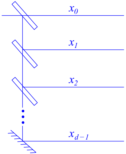
Figure 12: One way of instantiating $d$ spatial modes in an interferometer. A single photon is passed through the first beamsplitter from the left and is repeatedly split at $d-1$ beamsplitters, with the $(d-1)$th mode reflected by the mirror at the bottom.

To model this situation, the ontic state space is assumed to decompose into sets of ontic states $\Lambda^{(j)}$, which are localized at each mode, along with possibly some additional degrees of freedom $\Lambda_{\text{NL}}$ which are not so localized. The total ontic state space is then assumed to be $\Lambda=\left(\oplus_{j=0}^{d-1}\Lambda^{(j)}\right)\oplus\Lambda_{\text{NL}}$. As a concrete example, each mode might have exactly one ontic state, with the ontic state corresponding to mode $x_{j}$ labeled by the integer $j$. The ontic state space would then be $\{0,1,\cdots,d-1,\cdots\}=\{0\}\oplus\{1\}\oplus\cdots\oplus\{d-1\}\oplus\cdots$, where the second $\cdots$ is to leave room for possible additional ontic states not localized in a mode. More generally, the structure would be similar, but there could be multiple ontic states corresponding to each mode. Then, the state $\left[x_{j}\right]$ represents a situation in which only ontic states in $\Lambda^{(j)}$ can be occupied, so $\Lambda^{(j)}$ would be a measure one set according to any probability measure in $\Delta_{x_{j}}$.

Now, any unitary that leaves $\left[x_{0}\right]$ invariant can be implemented in such a way that it only involves manipulating modes $x_{1}$–$x_{d-1}$, say by adding phase shifters to them or combining them at beamsplitters. If implemented in this way, it makes sense, by locality, to think that this would have no effect on ontic states localized at $x_{0}$ and hence ontic indifference would be satisfied for $\left[x_{0}\right]$.

This argument for ontic indifference is based on locality, so it only works for states like $\left[x_{j}\right]$, which are spatially localized. Fortunately, Hardy’s Theorem can be proved under restricted ontic indifference, which only requires that ontic indifference should hold for a single pure state, so, in the case of our photon modes setup, this can always be chosen to be $\left[x_{0}\right]$. Hence the assumption need never be applied to a state that is not localized.

Even if the argument from locality were sound, we should be skeptical of imposing locality requirements on ontological models because of Bell’s Theorem. However, the argument can be evaded without even giving up on locality, since it is really the assumption that $\left[x_{j}\right]$ corresponds to a set of ontic states localized at $x_{j}$ that is at fault. Moving to a Fock space description, in which $\left[n\right]_{x_{j}}$ is the state in which there are $n$ photons in mode $x_{j}$, makes this objection clearer. In Fock space, the state $\left[x_{0}\right]$ is written as $\left[1\right]_{x_{0}}\otimes\left[0\right]_{x_{1}}\otimes\cdots\otimes\left[0\right]_{x_{d-1}}$, which explicitly shows that modes $x_{1}$–$x_{d-1}$ are in their vacuum state. From quantum field theory, we know that the vacuum is not a featureless void, but has some sort of structure. Therefore, it makes sense that, at the ontological level, there might be more than one ontic state associated with the vacuum, and a transformation that does not affect things localized at $x_{0}$ might still act nontrivially on these vacuum ontic states.

As an explicit example of this, we can construct a “second quantized” version of Spekkens’ toy theory, in which we allow each mode to have at most one photon. The states $\left[0\right]_{x_{j}}$, $\left[1\right]_{x_{j}}$, $\left[+\right]_{x_{j}}$, $\left[-\right]_{x_{j}}$, $\left[+i\right]_{x_{j}}$ and $\left[-i\right]_{x_{j}}$, where

$$\left|\pm\right\rangle =\frac{1}{\sqrt{2}}\left(\left|0\right\rangle\pm\left|1\right\rangle\right)$$ (208)

$$\left|\pm i\right\rangle =\frac{1}{\sqrt{2}}\left(\left|0\right\rangle\pm i\left|1\right\rangle\right),$$ (209)

are isomorphic to the states $\left[z+\right]$, $\left[z-\right]$, $\left[x+\right]$, $\left[x-\right]$, $\left[y+\right]$ and $\left[y-\right]$ of a spin-$1/2$ particle. Therefore, since Spekkens’ toy theory provides a model for these spin-$1/2$ states under measurements in the corresponding bases, it also provides a model for the corresponding photon states and measurements. In this model, the ontic state space for a mode is $\Lambda^{(j)}=\{(+,+)_{x_{j}},(+,-)_{x_{j}},(-,+)_{x_{j}},(-,-)_{x_{j}}\}$ and the ontic state spaces for modes compose via the Cartesian product rather than the direct sum. So, for example, in the case of two modes $x_{0}$ and $x_{1}$, the total ontic state space would be $\Lambda=\Lambda^{(0)}\times\Lambda^{(1)}$, which is

$$\{\left[(+,+)_{x_{0}},(+,+)_{x_{1}}\right],\left[(+,+)_{x_{0}},(+,-)_{x_{1}}\right],$$

$$\leavevmode\nobreak\ \left[(+,+)_{x_{0}},(-,+)_{x_{1}}\right],\left[(+,+)_{x_{0}},(-,-)_{x_{1}}\right],$$

$$\leavevmode\nobreak\ \left[(+,-)_{x_{0}},(+,+)_{x_{1}}\right],\left[(+,-)_{x_{0}},(+,-)_{x_{1}}\right],$$

$$\leavevmode\nobreak\ \left[(+,-)_{x_{0}},(-,+)_{x_{1}}\right],\left[(+,-)_{x_{0}},(-,-)_{x_{1}}\right],$$

$$\leavevmode\nobreak\ \left[(-,+)_{x_{0}},(+,+)_{x_{1}}\right],\left[(-,+)_{x_{0}},(+,-)_{x_{1}}\right],$$

$$\leavevmode\nobreak\ \left[(-,+)_{x_{0}},(-,+)_{x_{1}}\right],\left[(-,+)_{x_{0}},(-,-)_{x_{1}}\right],$$

$$\leavevmode\nobreak\ \left[(-,-)_{x_{0}},(+,+)_{x_{1}}\right],\left[(-,-)_{x_{0}},(+,-)_{x_{1}}\right],$$

$$\leavevmode\nobreak\ \left[(-,-)_{x_{0}},(-,+)_{x_{1}}\right],\left[(-,-)_{x_{0}},(-,-)_{x_{1}}\right]\}.$$ (210)

The vacuum state $\left[0\right]_{x_{j}}$ is represented by a equal mixture of $(+,+)_{x_{j}}$ and $(-,-)_{x_{j}}$, just like the $\left[z+\right]$ state in the spin-$1/2$ case, and the state $\left[1\right]_{x_{j}}$ with one photon is represented by an equal mixture of $(+,-)_{x_{j}}$ and $(-,+)_{x_{j}}$, just like the $\left[z-\right]$ state in the spin-$1/2$ case. The state $\left[x_{0}\right]=\left[1\right]_{x_{0}}\otimes\left[0\right]_{x_{1}}$ is then represented by the product of these two distributions, which is an equal mixture of $((+,-)_{x_{0}},(+,+)_{x_{1}})$, $((+,-)_{x_{0}},(-,-)_{x_{1}})$, $((-,+)_{x_{0}},(+,+)_{x_{1}})$ and $((-,+)_{x_{0}},(-,-)_{x_{1}})$. A transformation acting locally on $x_{1}$ can then switch the states $(+,+)_{x_{1}}$ and $(-,-)_{x_{1}}$, in violation of ontic indifference, whilst leaving the distribution invariant. Thus, the assumption that local ontic state spaces compose according to the direct sum, rather than locality per se., is the main problem with Hardy’s argument for ontic indifference. Since we expect vacuum states to have structure, this is not a good assumption on which to build a $\psi$-ontology theorem.

Nevertheless, the direct sum construction that motivates ontic indifference is closely related to the argument from interference discussed in §3.1. To see this connection, it is helpful to outline a simple special case of Hardy’s Theorem.

9.2 An example

Consider a Mach-Zehnder interferometer as depicted in Fig. 13. We will outline the argument that ontic indifference implies that the state $\left[x_{0}\right]$, representing a photon in the upper arm of the interferometer, must be ontologically distinct from $\left[\psi\right]$, where $\left|\psi\right\rangle=\frac{1}{\sqrt{2}}\left(\left|x_{0}\right\rangle+\left|x_{1}\right\rangle\right)$, representing an equal superposition of both paths. The argument in this section assumes a finite ontic state space. A measure-theoretic argument is given for the general case in the next section.

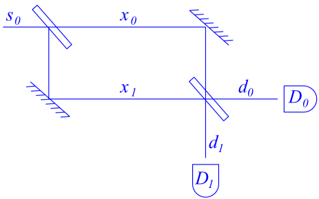
Figure 13: The Mach-Zehnder interferometer used in the example of Hardy’s Theorem.

On passing through the second beamsplitter, $\left|x_{0}\right\rangle$ gets mapped to $\frac{1}{\sqrt{2}}\left(\left|d_{0}\right\rangle+\left|d_{1}\right\rangle\right)$ and $\left|x_{1}\right\rangle$ gets mapped to $\frac{1}{\sqrt{2}}\left(\left|d_{0}\right\rangle-\left|d_{1}\right\rangle\right)$, from which we infer that $\left|\psi\right\rangle$ gets mapped to $\left|d_{0}\right\rangle$. Hence, if the state $\left[x_{0}\right]$ is prepared then the detectors $D_{0}$ and $D_{1}$ will fire with $50/50$ probability and if the state $\left[\psi\right]$ is prepared then $D_{0}$ will fire with certainty. For the practically inclined, note that the state $\left[\psi\right]$ can be prepared by passing a photon from the source $s_{0}$ through the first beamsplitter as in Fig. 13 and the state $\left[x_{0}\right]$ can be prepared by removing the first beamsplitter and passing a photon from $s_{0}$ directly into the upper arm.

The outcome of this experiment can be altered by placing a $\pi$ phase shifter in the lower arm of the interferometer, e.g. by altering its path length by half a wavelength relative to the upper arm. This leaves $\left|x_{0}\right\rangle$ invariant, but maps $\left|\psi\right\rangle$ to $\left|\phi\right\rangle=\frac{1}{\sqrt{2}}\left(\left|x_{0}\right\rangle-\left|x_{1}\right\rangle\right)$, which will now cause the detector $D_{1}$ to fire with certainty. This is a typical example of interference, replacing constructive interference ($D_{0}$ fires without the phase shifter) with destructive interference ($D_{1}$ fires with the phase shifter).

In an ontological model, assume that there is some ontic state $\lambda$ that is assigned nonzero probability by both $\left[x_{0}\right]$ and $\left[\psi\right]$. We will show that, under the assumption of ontic indifference, this leads to a contradiction.

Since $\left[\psi\right]$ and $\left[\phi\right]$ are orthogonal, by Theorem 4.10 they must be ontologically distinct. This can also be seen more directly because every ontic state assigned nonzero probability by $\left[\psi\right]$ must cause $D_{0}$ to fire with certainty, whereas every ontic state assigned nonzero probability by $\left[\phi\right]$ must cause $D_{1}$ to fire with certainty. Therefore, $\left[\phi\right]$ must assign zero probability to the ontic state $\lambda$.

Now consider the action of the unitary $U$ that adds a $\pi$ phase shift to the mode $x_{1}$. Since this leaves $\left[x_{0}\right]$ invariant, the assumption of ontic indifference implies that $\lambda$ must be left invariant. However, since $U$ maps $\left[\psi\right]$ to $\left[\phi\right]$, it must also cause $\lambda$ to transition to an ontic state that causes $D_{1}$ to fire with certainty, and no such ontic state has nonzero probability according to $\left[\psi\right]$. Therefore $\lambda$ cannot be left invariant, which is a contradiction. We conclude that there can be no $\lambda$ assigned nonzero probability by both $\left[x_{0}\right]$ and $\left[\psi\right]$.

By considering Hardy’s motivation for ontic indifference, this can be connected to the argument from interference as follows. Assume that the ontic state space decomposes into a direct sum $\Lambda=\Lambda^{(0)}\oplus\Lambda^{(1)}\oplus\Lambda_{\text{NL}}$. The states in $\Lambda^{(0)}$ are localized in the upper arm of the interferometer, representing the photon definitely taking the upper path, and the states in $\Lambda^{(1)}$ are localized in the lower arm of the interferometer, representing the photon definitely taking the lower path. If we assume that the placement of a $\pi$ phase shifter in the lower arm has no effect on the ontic states in $\Lambda^{(0)}$ then we can deduce that $\left[\psi\right]$ cannot assign nonzero probability to states in $\Lambda^{(0)}$ by the same argument as above. Switching the roles of $x_{0}$ and $x_{1}$, so that the phase shifter is now placed or not placed in $x_{0}$, we can deduce the same for $\Lambda^{(1)}$. Therefore, $\left[\psi\right]$ must assign all its weight to $\Lambda_{\text{NL}}$, which is not localized to either arm. You could say that this represents a situation in which the photon “travels along both paths”, but it would be more accurate to say that it only has global degrees of freedom, not localized on either path. Further, if we assume that $\left[x_{0}\right]$ and $\left[x_{1}\right]$ are entirely supported on $\Lambda^{(0)}$ and $\Lambda^{(1)}$ respectively, then the three quantum states $\left[\psi\right]$, $\left[x_{0}\right]$ and $\left[x_{1}\right]$ must be ontologically distinct. This is a bit further along the road to proving $\psi$-ontology than the more naive version of the argument from interference. Hardy’s result then shows that the same sort of assumption can be used to prove a full blown $\psi$-ontology theorem, which seems to vindicate the intuition behind the argument from interference.

Of course, if we give up the idea that the ontic state space must decompose as a direct sum of local state spaces plus some global degrees of freedom, then there is no motivation for ontic indifference, so the above argument does not go through. In fact, the second quantized version of Spekkens’ toy theory is able to account for almost all the qualitative features of Mach-Zehnder interferometry in a local and $\psi$-epistemic way [91]. Thus, any claim that these experiments entail the reality of the wavefunction or violate locality must involve implicitly assuming something like ontic indifference. The most important aspect of Hardy’s analysis is to bring this assumption to the fore more clearly.

9.3 The main result

We are now in a position to state and prove Hardy’s main result. The proof strategy used here is due to Patra, Pironio and Massar [60] and is conceptually simpler than Hardy’s original proof.

Theorem 9.2.

Let $\mathcal{P}$ be the set of pure states on $\mathbb{C}^{d}$ for $d\geq 3$. Then, there exists a set of measurements $\mathcal{M}$ and a set of unitaries $\mathcal{T}$ such that any ontological model of the PMT fragment $\mathfrak{F}=\langle\mathbb{C}^{d},\mathcal{P},\mathcal{M},\mathcal{T}\rangle$ that reproduces the quantum preclusions and satisfies restricted ontic indifference has the property that any pair of states $\left[\psi\right],\left[\phi\right]\in\mathcal{P}$ satisfying $\text{Tr}\left(\left[\phi\right]\left[\psi\right]\right)\leq(d-1)/d$ must be ontologically distinct.

Before proving this theorem, note that, if we form a product of $\mathfrak{F}$ with another fragment $\mathfrak{F}^{\prime}$ and assume that there exits an ontological model of the larger fragment that reproduces the quantum preclusions and preserves ontological distinctness with respect to our ontological model of $\mathfrak{F}$, then, for any pair $\left[\psi\right],\left[\phi\right]\in\mathcal{P}$, we can always choose the dimensionality of the Hilbert space of $\mathfrak{F}^{\prime}$ such that $\text{Tr}\left(\left[\phi\right]\otimes\left[0\right]\left[\psi\right]\otimes\left[0\right]\right)\leq(d-1)/d$ is satisfied, where $\left[0\right]$ is any fixed pure state of $\mathfrak{F}^{\prime}$. Hardy’s Theorem implies that $\left[\psi\right]\otimes\left[0\right]$ and $\left[\phi\right]\otimes\left[0\right]$ must be ontologically distinct, and then the assumption that appending ancillas preserves ontological distinctness implies that $\left[\psi\right]$ and $\left[\phi\right]$ must be ontologically distinct in the original model. Since this applies to any pair of pure states, the original ontological model must be $\psi$-ontic. The case $d=2$ is dealt with in a similar way.

The proof relies on the following three lemmas.

Lemma 9.3.

Let $\mathfrak{F}=\langle\mathcal{H},\mathcal{P},\mathcal{M},\mathcal{T}\rangle$ be a PMT fragment, let $\Theta=(\Lambda,\Sigma,\Delta,\Xi,\Gamma)$ be an ontological model of it, let $\left[\psi\right]$ be a state that satisfies ontic indifference in $\Theta$, let $\{U_{j}\}\subseteq\mathcal{T}$ be an at most countable set of unitaries that leave $\left[\psi\right]$ invariant and suppose that $\left[\phi\right]$ is ontologically indistinct from $\left[\psi\right]$ in $\Theta$. Then there exist measures $\mu_{j}\in\Delta_{U_{j}\left[\phi\right]U_{j}^{\dagger}}$, such that $L(\{\mu_{j}\})>0$, where $L$ is the overlap.

Proof.

Let $\nu\in\Delta_{\psi}$ and suppose that $\Omega_{j}$ is a measure one set left invariant by some $\gamma^{j}\in\Gamma_{U_{j}}$, i.e. $\gamma^{j}_{\lambda}(\Omega_{j}^{\prime})=\delta_{\lambda}(\Omega_{j}^{\prime})$ for $\lambda\in\Omega_{j}$ and $\Omega_{j}^{\prime}\subseteq\Omega_{j}$. Then, $\Omega=\cap_{j}\Omega_{j}$ is also measure one according to $\nu$ because it is the intersection of an at most countable set of measure one sets, and $\Omega$ is left invariant by each $\gamma^{j}$. Since $\left[\psi\right]$ and $\left[\phi\right]$ are ontologically indistinct, there exists a $\mu\in\Delta_{\phi}$ such that $\mu(\Omega)>0$. Now, the measure $\mu_{j}$, defined by $\mu_{j}(\Omega^{\prime})=\int_{\Lambda}\gamma^{j}_{\lambda}(\Omega^{\prime})d\mu(\lambda)$ for $\Omega^{\prime}\in\Sigma$, is in $\Delta_{U_{j}\left[\phi\right]U_{j}^{\dagger}}$, and $\mu_{j}(\Omega^{\prime})=\mu(\Omega^{\prime})$ for $\Omega^{\prime}\subseteq\Omega$.

Now, consider a partition of $\Lambda$ into sets $\Omega^{k}$. Then,

$$\sum_{k}\min_{j}\left[\mu_{j}(\Omega^{k})\right]$$

$$=\sum_{k}\min_{j}\left[\mu_{j}\left(\Omega^{k}\cap\Omega\right)+\mu_{j}\left(\Omega^{k}\cap\left(\Lambda\backslash\Omega\right)\right)\right]$$ (211)

$$\geq\sum_{k}\left(\min_{j}\left[\mu_{j}\left(\Omega^{k}\cap\Omega\right)\right]+\min_{j}\left[\mu_{j}\left(\Omega^{k}\cap\left(\Lambda\backslash\Omega\right)\right)\right]\right)$$ (212)

$$\geq\sum_{k}\min_{j}\left[\mu_{j}\left(\Omega^{k}\cap\Omega\right)\right]$$ (213)

$$=\sum_{k}\mu(\Omega^{k}\cap\Omega)=\mu(\Omega)>0.$$ (214)

Since this holds for all partitions it must also hold for the infimum, and hence $L(\{\mu_{j}\})>0$. ∎

The next lemma is also used in the proof of the Colbeck–Renner Theorem.

Lemma 9.4.

Let $\left\{\left|j\right\rangle\right\}_{j=0}^{d-1}$ be a set of $d\geq 3$ orthonormal vectors in $\mathbb{C}^{d^{\prime}}$ for $d^{\prime}\geq d$, i.e. not necessarily a complete basis, and consider the vectors

$$\left|\psi\right\rangle=\frac{1}{\sqrt{d}}\sum_{j=0}^{d-1}\left|j\right\rangle,$$ (215)

and

$$\left|\phi\right\rangle=\frac{1}{\sqrt{d-1}}\sum_{j=1}^{d-1}e^{\imath\varphi_{j}}\left|j\right\rangle.$$ (216)

Then, the phases $\varphi_{j}$ may be chosen such that $\left\langle\phi\middle|\psi\right\rangle$ is real and takes any value between $0$ and $\sqrt{\frac{d-1}{d}}$.

Proof.

First consider the case where $d$ is odd. In this case, set $\varphi_{j}=\varphi$ for $1\leq j\leq\frac{d-1}{2}$ and $\varphi_{j}=-\varphi$ for $\frac{d+1}{2}\leq j\leq{d-1}$. Then, $\left\langle\phi\middle|\psi\right\rangle=\sqrt{\frac{d-1}{d}}\cos\varphi$, which may take any value between $0$ and $\sqrt{\frac{d-1}{d}}$ by varying $\varphi$ from $0$ to $\pi/2$.

When $d$ is even, set $\varphi_{1}=0$, $\varphi_{j}=\phi$ for $2\leq j\leq\frac{d}{2}$, and $\varphi_{j}=-\phi$ for $\frac{d}{2}+1\leq j\leq{d-1}$. Then, $\left\langle\phi\middle|\psi\right\rangle=\sqrt{\frac{1}{d(d-1)}}(1+(d-2)\cos\varphi)$. This is equal to $\sqrt{\frac{d-1}{d}}$ for $\varphi=0$ and is equal to $0$ for $\varphi=\pi-\cos^{-1}\left(\frac{1}{d-2}\right)$ and varies continuously in between, so again any positive real number between $0$ and $\sqrt{\frac{d-1}{d}}$ can be obtained. ∎

Lemma 9.5.

Let $\left[\psi\right]$ and $\left[\phi\right]$ be two nonorthogonal states on $\mathbb{C}^{d}$ for $d\geq 3$ such that $\text{Tr}\left(\left[\phi\right]\left[\psi\right]\right)\leq(d-1)/d$. Then, there exist unitaries $\{U_{j}\}_{j=0}^{d-1}$ such that $U_{j}\left[\psi\right]U_{j}^{\dagger}=\left[\psi\right]$ and such that $\{\left[\phi_{j}\right]\}$ is antidistinguishable, where $\left[\phi_{j}\right]=U_{j}\left[\phi\right]U_{j}^{\dagger}$.

Proof.

Let $\left|\psi\right\rangle$ and $\left|\phi\right\rangle$ be vector representatives of $\left[\psi\right]$ and $\left[\phi\right]$. Then,

$$\left|\phi\right\rangle=\alpha\left|\psi\right\rangle+\beta\left|\psi^{\perp}\right\rangle,$$ (217)

where $\alpha=\left\langle\phi\middle|\psi\right\rangle$ and $\left\langle\psi^{\perp}\middle|\psi\right\rangle=0$. By appropriate choice of the global phase of $\left|\psi\right\rangle$, it is possible to make $\alpha$ real and positive.

Let $\left\{\left|j\right\rangle\right\}_{j=0}^{d-1}$ be a basis in which $\left|\psi\right\rangle$ is represented as $\left|\psi\right\rangle=\frac{1}{\sqrt{d}}\sum_{j=0}^{d-1}\left|j\right\rangle$ and consider the vector

$$\left|\phi_{0}\right\rangle=\frac{1}{\sqrt{d-1}}\sum_{j=0}^{d-1}e^{\imath\varphi_{j}}\left|j\right\rangle.$$ (218)

By Lemma 9.4, it is possible to choose the phases $\varphi_{j}$ such that $\left\langle\phi_{0}\middle|\psi\right\rangle=\alpha$, since $\alpha$ is between $0$ and $\sqrt{\frac{d-1}{d}}$.

Making this choice of phases, it follows that

$$\left|\phi_{0}\right\rangle=\alpha\left|\psi\right\rangle+\beta\left|\psi^{\perp}_{0}\right\rangle,$$ (219)

where $\left\langle\psi^{\perp}_{0}\middle|\psi\right\rangle=0$. Let $U$ be a unitary that acts as $U\left|\psi\right\rangle=\left|\psi\right\rangle$ and $U\left|\psi^{\perp}\right\rangle=\left|\psi^{\perp}_{0}\right\rangle$. It follows that $\left|\phi_{0}\right\rangle=U\left|\phi\right\rangle$.

Now, consider the unitary $V$, where $V\left|j\right\rangle=\left|j+1\mod d\right\rangle$, which leaves $\left|\psi\right\rangle$ invariant. Then, $U_{j}=V^{j}U$ also leaves $\left|\psi\right\rangle$ invariant for $j=0,1,\ldots,d-1$ and the vectors $\left|\phi_{j}\right\rangle=U_{j}\left|\psi\right\rangle$ satisfy $\left\langle j\middle|\phi_{j}\right\rangle=0$, since, by construction, $\left\langle 0\middle|\phi_{0}\right\rangle=0$. Thus, the states $\left\{\left[\phi_{j}\right]\right\}_{j=0}^{d-1}$ are antidistinguished by the measurement $\left\{\left[j\right]\right\}_{j=0}^{d-1}$ as required. ∎

Proof of Theorem 9.2.

Let $\Theta=(\Lambda,\Sigma,\Delta,\Xi,\Gamma)$ be an ontological model of the PMT fragment $\mathfrak{F}$ to be constructed. For the purposes of contradiction, assume that two states $\left[\psi\right],\left[\phi\right]\in\mathcal{P}$ satisfying $\text{Tr}\left(\left[\phi\right]\left[\psi\right]\right)\leq(d-1)/d$ are ontologically indistinct in $\Theta$ and let $\left[\psi^{\prime}\right]$ be a state that satisfies ontic indifference in $\Theta$. Without loss of generality, we may assume that $\left[\psi\right]=\left[\psi^{\prime}\right]$. If not, let $U$ be a unitary such that $\left[\psi^{\prime}\right]=U\left[\psi\right]U^{\dagger}$ and assume $U\in\mathcal{T}$. Then the states $\left[\psi^{\prime}\right]$ and $\left[\phi^{\prime}\right]=U\left[\phi\right]U^{\dagger}$ satisfy $\text{Tr}\left(\left[\phi^{\prime}\right]\left[\psi^{\prime}\right]\right)\leq(d-1)/d$ because the inner product is preserved under unitary transformations. Also, by Corollary 8.4, if $\left[\psi\right]$ and $\left[\phi\right]$ are ontologically indistinct then so are $\left[\psi^{\prime}\right]$ and $\left[\phi^{\prime}\right]$ so it is sufficient to derive a contradiction for these two states.

By Lemma 9.5, there exist unitaries $\{U_{j}\}_{j=0}^{d-1}$ that leave $\left[\psi\right]$ invariant such that $\left\{U_{j}\left[\phi\right]U_{j}^{\dagger}\right\}_{j=0}^{d-1}$ is antidistinguishable. Assume that each $U_{j}$ is in $\mathcal{T}$ and that the antidistinguishing measurement is in $\mathcal{M}$. Then, by Theorem 6.5, for every set of probability measures $\{\mu_{j}\}_{j=0}^{d-1}$ with $\mu_{j}\in\Delta_{U_{j}\left[\phi\right]U_{j}^{\dagger}}$, $L(\{\mu_{j}\})=0$, but by Lemma 9.3 there must exist a set such that $L(\{\mu_{j}\})>0$. Thus, we have a contradiction so $\left[\psi\right]$ and $\left[\phi\right]$ must be ontologically distinct. ∎

10 The Colbeck–Renner Theorem

Our final $\psi$-ontology theorem is due to Colbeck and Renner [122]. They originally proved a $\psi$-ontology theorem as a byproduct of a broader no-go theorem that aimed to rule out any ontological model of quantum theory in which more precise predictions can be made given knowledge of the ontic state than if you only know the quantum state [123, 124, 50]. This broader theorem is quite tricky to understand, both conceptually and technically, and its assumptions have been criticized [125, 126, 127]. Fortunately, Colbeck and Renner have recently put forward a simplified argument for $\psi$-ontology based on similar ideas that bypasses much of the complexity [122]. I present my own variation of the proof here.

The Colbeck–Renner Theorem is based on a locality assumption known as parameter independence. The condition of Bell locality, discussed in §5.4, can be decomposed as the conjunction of parameter independence and another assumption called outcome independence. Roughly speaking, parameter independence says that the measurement outcome at Bob’s side should not depend on Alice’s choice of measurement, and outcome independence says that the measurement outcome at Bob’s side should not depend on Alice’s measurement outcome. For a typical Bell inequality experiment, it is in principle possible to reproduce the quantum predictions by violating outcome independence and leaving parameter independence intact, so the Colbeck–Renner Theorem rules out the class of $\psi$-epistemic models that opt for this resolution to the conundrum presented by Bell’s Theorem. Nevertheless, Bell’s Theorem should lead us to be skeptical of imposing locality assumptions on ontological models. Indeed, many notable realist approaches to quantum theory, such as de Broglie–Bohm theory, violate parameter independence. As well as ruling out $\psi$-epistemic models, parameter independence rules out a wide class of viable $\psi$-ontic models, so it is perhaps an unreasonably strong assumption for a $\psi$-ontology theorem.

It should be noted that Colbeck and Renner claim that their theorem is not directly based on parameter independence, but rather on a broader assumption that they call “free choice”, aimed at capturing the idea that certain variables, such as the settings of preparation and measurement devices, are chosen freely by the experimenter and not constrained by other parameters of the system. Parameter independence is just one consequence of their free choice assumption. However, whether their assumption truly captures the meaning of making a free choice is one of the most controversial aspects of the Colbeck–Renner argument. My own opinion is that, whilst some aspects of free choice are captured by the Colbeck–Renner assumption, it is at least partly a locality assumption as well because it implies parameter independence. Therefore, I prefer to avoid the free choice controversy and just assume parameter independence directly.

Understanding the Colbeck–Renner Theorem requires quite a bit of background material, so the discussion is broken down into four sections. §10.1 gives a formal definition of parameter independence and shows how, given an ontological model for a bipartite system, it can be used to derive an ontological model for the reduced states on a subsystem. §10.2 introduces chained Bell measurements, which are the main technical tool used in proving the Colbeck–Renner Theorem. §10.3 discusses the equiprobability theorem, which shows that, in a model that satisfies parameter independence, all ontic states associated with a maximally entangled state must assign equal probability to all the outcomes of some local measurement in an orthonormal basis. Finally, §10.4 leverages the equiprobability theorem to prove the main result.

10.1 Parameter Independence

As in Bell’s Theorem, the fragment of interest for the Colbeck–Renner Theorem is a product measurement fragment, consisting of states and local measurements on a bipartite system (see Definition 5.6). §5.4 discussed the concept of a conditional fragment on Bob’s system that results from viewing Alice’s measurements as preparation procedures for states on Bob’s system. Given an ontological model for a product measurement fragment that satisfies Bell locality, it is possible to derive a model for the conditional fragment from it. Here, we are concerned with a smaller fragment that results from tracing out one of the systems, but not post-selecting on measurement outcomes.

Definition 10.1.

Let $\mathfrak{F}_{AB}=\langle\mathcal{H}_{A}\otimes\mathcal{H}_{B},\mathcal{P}_{AB},\mathcal{M}_{A}\times\mathcal{M}_{B}\rangle$ be a product measurement fragment. The marginal fragment on $A$ is $\mathfrak{F}_{A}=\langle\mathcal{H}_{A},\mathcal{P}_{A},\mathcal{M}_{A}\rangle$, where $\mathcal{P}_{A}$ consists of all states of the form $\rho_{A}=\text{Tr}_{B}\left(\rho_{AB}\right)$ for $\rho_{AB}\in\mathcal{P}_{AB}$. The marginal fragment on $B$ is defined similarly, with the roles of $A$ and $B$ interchanged.

In general, an ontological model $\Theta_{AB}=(\Lambda_{AB},\Sigma_{AB},\Delta_{AB},\Xi_{AB})$ for a product measurement fragment $\mathfrak{F}_{AB}=\langle\mathcal{H}_{A}\otimes\mathcal{H}_{B},\mathcal{P}_{AB},\mathcal{M}_{A}\times\mathcal{M}_{B}\rangle$ specifies a set of conditional probability distributions $\text{Pr}_{AB}\in\Xi_{AB}[M_{A},\allowbreak M_{B}]$ for every $M_{A}\in\mathcal{M}_{A}$ and $M_{B}\in\mathcal{M}_{B}$. These distributions are of the form $\text{Pr}_{AB}(E,F|M_{A},M_{B},\lambda)$, where $E$ varies over $M_{A}$ and $F$ varies over $M_{B}$. If the model reproduces the quantum predictions, then for all $\rho_{AB}\in\mathcal{P}_{AB}$, $M_{A}\in\mathcal{M}_{A}$, $M_{B}\in\mathcal{M}_{B}$, $E\in M_{A}$ and $F\in M_{B}$,

$$\int_{\Lambda_{AB}}\text{Pr}_{AB}(E,F|M_{A},M_{B},\lambda)d\mu(\lambda)=\text{Tr}_{AB}\left(E\otimes F\rho_{AB}\right),$$ (220)

for every $\mu\in\Delta_{AB}[\rho]$ and $\text{Pr}_{AB}\in\Xi_{AB}[M_{A},M_{B}]$. Summing both sides of this equation over $F\in M_{B}$ gives

$$\int_{\Lambda_{AB}}\text{Pr}_{AB}(E|M_{A},M_{B},\lambda)d\mu(\lambda)=\text{Tr}_{A}\left(E\rho_{A}\right),$$ (221)

where $\rho_{A}=\text{Tr}_{B}\left(\rho_{AB}\right)$ and $\text{Pr}_{AB}(E|M_{A},M_{B},\lambda)=\sum_{F\in M_{B}}\text{Pr}_{AB}(E,F|M_{A},M_{B},\lambda)$. For a fixed $M_{B}$, $\text{Pr}_{AB}(E|M_{A},M_{B},\lambda)$ is a valid conditional probability distribution over $M_{A}$ that could be used in an ontological model of the marginal fragment. Further, if $\mu$ is used to represent $\rho_{A}$, this choice of conditional probability distributions reproduces the quantum predictions. The only difficulty is that $\text{Pr}_{AB}(E|M_{A},M_{B},\lambda)$ depends on $M_{B}$ as well as $M_{A}$, so there is an ambiguity about which choice of $M_{B}$ should be used to model the marginal fragment. The assumption of parameter independence removes this ambiguity.

Definition 10.2.

An ontological model $\Theta_{AB}=(\Lambda_{AB},\Sigma_{AB},\Delta_{AB},\xi_{AB})$ of a product measurement fragment $\mathfrak{F}_{AB}=\langle\mathcal{H}_{A}\otimes\mathcal{H}_{B},\mathcal{P}_{AB},\mathcal{M}_{A}\times\mathcal{M}_{B}\rangle$ satisfies parameter independence if, for all $M_{A}\in\mathcal{M}_{A}$, $M_{B}\in\mathcal{M}_{B}$ and $\text{Pr}_{AB}\in\Xi_{AB}[M_{A},M_{B}]$,

$$\text{Pr}_{AB}(E|M_{A},M_{B},\lambda) =\text{Pr}_{AB}(E|M_{A},\lambda)$$ (222)

$$\text{Pr}_{AB}(F|M_{A},M_{B},\lambda) =\text{Pr}_{AB}(F|M_{B},\lambda).$$ (223)

Parameter independence is a locality assumption that says that Alice’s measurement outcome should not depend on Bob’s choice of measurement and vice versa. It is a weaker requirement than Bell locality, as it can be shown that the conjunction of parameter independence and outcome independence, which reads

$$\text{Pr}_{AB}(E|M_{A},M_{B},F,\lambda) =\text{Pr}_{AB}(E|M_{A},M_{B},\lambda)$$ (224)

$$\text{Pr}_{AB}(F|M_{A},E,M_{B},\lambda) =\text{Pr}_{AB}(F|M_{A},M_{B},\lambda),$$ (225)

is equivalent to Bell locality [128, 129]. For present purposes, the point of this is that, whilst the full Bell locality condition is needed to derive a well-defined ontological model for conditional fragments, parameter independence is sufficient to have unambiguous models for marginal fragments.

Definition 10.3.

Let $\mathfrak{F}_{AB}=\langle\mathcal{H}_{A}\otimes\mathcal{H}_{B},\mathcal{P}_{AB},\mathcal{M}_{A}\times\mathcal{M}_{B}\rangle$ be a product measurement fragment and let $\Theta_{AB}=(\Lambda_{AB},\Sigma_{AB},\Delta_{AB},\Xi_{AB})$ be an ontological model of it that satisfies parameter independence. The marginal model on $A$, $\Theta_{A}=(\Lambda_{AB},\Sigma_{AB},\Delta_{A},\Xi_{A})$ is an ontological model for the marginal fragment $\mathfrak{F}_{A}=\langle\mathcal{H}_{A},\mathcal{P}_{A},\mathcal{M}_{A}\rangle$, where, for $\rho_{A}\in\mathcal{P}_{A}$,

$$\Delta_{A}[\rho_{A}]=\cup_{\{\rho_{AB}\in\mathcal{P}_{AB}|\text{Tr}_{B}\left(\rho_{AB}\right)=\rho_{A}\}}\Delta_{AB}[\rho_{AB}],$$ (226)

and $\Xi_{A}[M_{A}]$ consists of all conditional probability distributions of the form

$$\text{Pr}_{A}(E|M_{A},\lambda)=\sum_{F\in M_{B}}\text{Pr}_{AB}(E,F|M_{A},M_{B},\lambda),$$ (227)

for all $\text{Pr}_{AB}\in\Xi_{AB}[M_{A},M_{B}]$. Note that, by parameter independence, these distributions are independent of $M_{B}$.

Eq. (221) implies that if $\Theta_{AB}$ reproduces the quantum predictions for $\mathfrak{F}_{AB}$ then the marginal model $\Theta_{A}$ reproduces the quantum predictions for the marginal fragment $\mathfrak{F}_{A}$.

10.2 Chained Bell measurements

The main engine of the proof of the Colbeck–Renner Theorem is the chained Bell measurements. These were originally developed in the context of a proof of Bell’s Theorem that involved chaining together several tests of the Clauser–Horne–Shimony–Holt inequality [130], resulting in the chained Bell inequalities [131, 132], which explains the terminology.

We are interested in the product measurement fragment $\mathfrak{F}=\langle\mathcal{H}_{A}\otimes\mathcal{H}_{B},\mathcal{P}_{AB},\mathcal{M}_{A}\times\mathcal{M}_{B}\rangle$, where $\mathcal{H}_{A}=\mathcal{H}_{B}=\mathbb{C}^{2}$ and both $\mathcal{M}_{A}$ and $\mathcal{M}_{B}$ contain $N$ measurements in orthonormal bases. For later convenience, Alice’s measurements are labeled by even integers and Bob’s by the odd integers, so we have $M_{A}^{a}\in\mathcal{M}_{A}$ for $a\in E_{N}=\{0,2,\ldots,2N-2\}$ and $M_{A}^{b}\in\mathcal{M}_{B}$ for $b\in O_{N}=\{1,3,\ldots,2N-1\}$. The measurements are described by pairs of orthogonal rank-1 projectors $M_{A}^{a}=\{\left[\phi^{a}_{0}\right]_{A},\left[\phi^{a}_{1}\right]_{A}\}$, $M_{B}^{b}=\{\left[\phi^{b}_{0}\right]_{B},\left[\phi^{b}_{1}\right]_{B}\}$ onto the orthonormal bases $\left\{\left|\phi^{a}_{0}\right\rangle_{A},\left|\phi^{a}_{1}\right\rangle_{A}\right\}$ and $\left\{\left|\phi^{b}_{0}\right\rangle_{B},\left|\phi^{b}_{1}\right\rangle_{B}\right\}$. If the state $\rho_{AB}$ is prepared, Alice measures $M_{A}^{a}$, and Bob measures $M_{B}^{b}$, then the outcome probabilities are

$$\text{Prob}\left(\left[\phi^{a}_{j}\right],\left[\phi^{b}_{k}\right]|M_{A}^{a},M_{B}^{b},\rho_{AB}\right)=\text{Tr}_{AB}\left(\left[\phi^{a}_{j}\right]\otimes\left[\phi^{b}_{k}\right]\rho_{AB}\right).$$ (228)

For later convenience, we introduce two random variables $X$ and $Y$ that take values $0$ and $1$ to represent Alice and Bob’s outcomes and write

$$\text{Prob}(X=j,Y=k|a,b,\rho_{AB})$$

$$\quad=\text{Prob}\left(\left[\phi^{a}_{j}\right],\left[\phi^{b}_{k}\right]|M_{A}^{a},M_{B}^{b},\rho_{AB}\right).$$ (229)

Now consider the following correlation measure for these outcome probabilities.

$$I_{N}(\rho_{AB})=\text{Prob}(X=Y|0,2N-1,\rho_{AB})$$

$$\quad+\sum_{\left\{(a,b)\middle|a\in E_{N},b\in O_{N},|a-b|=1\right\}}\text{Prob}(X\neq Y|a,b,\rho_{AB}).$$ (230)

The structure of this measure is illustrated in Fig. 14. Note that smaller values of this measure indicate that the measurement outcomes are more highly correlated.

Now, let $\left\{\left|0\right\rangle,\left|1\right\rangle\right\}$ be an orthonormal basis for $\mathbb{C}^{2}$, and consider the quantum state $\left[\Phi^{+}\right]_{AB}$, where

$$\left|\Phi^{+}\right\rangle_{AB}=\frac{1}{\sqrt{2}}\left(\left|0\right\rangle_{A}\otimes\left|0\right\rangle_{B}+\left|1\right\rangle_{A}\otimes\left|1\right\rangle_{B}\right).$$ (231)

Let $\vartheta^{a}_{j}=\left(\frac{a}{2N}+j\right)\pi$, and suppose that the bases for Alice and Bob’s measurements are given by

$$\left|\phi^{a}_{j}\right\rangle_{A} =\cos\left(\frac{\vartheta^{a}_{j}}{2}\right)\left|0\right\rangle_{A}+\sin\left(\frac{\vartheta^{a}_{j}}{2}\right)\left|1\right\rangle_{A}$$ (232)

$$\left|\phi^{b}_{k}\right\rangle_{B} =\cos\left(\frac{\vartheta^{b}_{k}}{2}\right)\left|0\right\rangle_{A}+\sin\left(\frac{\vartheta^{b}_{k}}{2}\right)\left|1\right\rangle_{B}.$$ (233)

The $j,k=0$ outcomes of these measurements are illustrated on the Bloch sphere in Fig. 15.

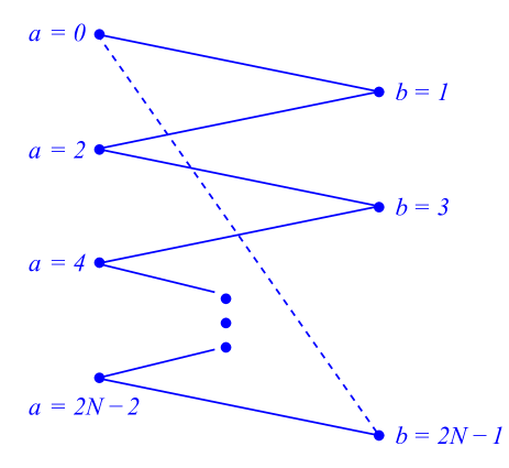
Figure 14: The structure of the correlation measure given in Eq. (10.2). A solid line between $a$ and $b$ represents the probability that the outcomes of $M^{A}_{a}$ and $M^{A}_{b}$ are different and a dotted line represents the probability that they are the same. The correlation measure is then the sum of the terms represented by each line.

With these particular choices, the outcome probabilities are

$$\text{Prob}\left(X=j,Y=k|a,b,\left[\Phi^{+}\right]_{AB}\right)$$

$$\quad=\frac{1}{2}\cos^{2}\left(\left(\frac{a-b}{2N}+j-k\right)\frac{\pi}{2}\right),$$ (234)

from which it is straightforward to compute that

$$I_{N}(\left[\Phi^{+}_{AB}\right])=2N\sin^{2}\frac{\pi}{4N}\leq\frac{\pi^{2}}{8N},$$ (235)

so that the correlation measure tends to zero as $N\rightarrow\infty$.

Without going through the whole calculation, it is fairly easy to see why this should be the case. For the state $\left[\Phi^{+}\right]_{AB}$, when Alice performs the measurement $M_{A}^{a}$ and obtains the outcome $j$, Bob’s state gets updated to $\left[\phi^{a}_{j}\right]_{B}$. The condition $|a-b|=1$ in the sum in Eq. (10.2) means that, in the limit of large $N$, the terms in this sum involve basis states for Bob that are very close to Alice’s basis states. Thus, since Bob’s system collapses to the basis state that Alice obtained in her measurement, the probability of getting the same outcome is very high, and hence $P(X\neq Y|a,b,\left[\Phi^{+}\right]_{AB})$ is close to zero. Similarly, the state $\left[\phi_{j}^{2N-1}\right]_{B}$ is almost orthogonal to $\left[\phi_{j}^{0}\right]_{B}$, so the probability of getting equal outcomes in the first term is also close to zero.

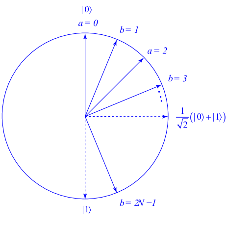
Figure 15: Alice and Bob’s measurement bases represented on a great circle of the Bloch sphere.

10.3 The equiprobability theorem

The aim of this section is to prove the main technical result that the Colbeck–Renner Theorem relies upon. We first deal with the case where Alice and Bob’s Hilbert spaces are two dimensional, and then extend this to higher dimensions.

Theorem 10.4.

Let $\mathfrak{F}_{AB}=\langle\mathcal{H}_{A}\otimes\mathcal{H}_{B},\mathcal{P}_{AB},\mathcal{M}_{A}\times\mathcal{M}_{B}\rangle$ be a product measurement fragment where $\mathcal{H}_{A}=\mathcal{H}_{B}=\mathbb{C}^{2}$, $\mathcal{P}_{AB}$ contains the maximally entangled state $\left[\Phi^{+}\right]_{AB}$, where

$$\left|\Phi^{+}\right\rangle_{AB}=\frac{1}{\sqrt{2}}\left(\left|0\right\rangle_{A}\otimes\left|0\right\rangle_{B}+\left|1\right\rangle_{A}\otimes\left|1\right\rangle_{B}\right),$$ (236)

for some orthonormal basis $\left\{\left|0\right\rangle,\left|1\right\rangle\right\}$, $\mathcal{M}_{A}$ contains measurements in every orthonormal basis on $\mathcal{H}_{A}$ and $\mathcal{M}_{B}$ contains measurements in every orthonormal basis on $\mathcal{H}_{B}$.

Let $\Theta_{AB}=(\Lambda_{AB},\Sigma_{AB},\Delta_{AB},\Xi_{AB})$ be an ontological model of $\mathfrak{F}_{AB}$ that reproduces the quantum predictions and satisfies parameter independence.

Then, for any $\mu\in\Delta_{AB}\left[\left[\Phi^{+}\right]_{AB}\right]$, there exists a set $\Omega\in\Sigma_{AB}$ such that $\mu(\Omega)=1$ and, for the measurement $M_{A}=\left\{\left[0\right]_{A},\left[1\right]_{A}\right\}$, all $\mathrm{Pr}_{A}\in\Xi_{A}[M_{A}]$ in the marginal model on $A$ satisfy $\mathrm{Pr}_{A}\left(\left[0\right]_{A}\middle|M_{A},\lambda\right)=\mathrm{Pr}_{A}\left(\left[1\right]_{A}\middle|M_{A},\lambda\right)=\frac{1}{2}$ for $\lambda\in\Omega$.

Before proving this theorem, it is instructive to see how it can be used to establish ontological distinctness for some pairs of states. Consider the state $\left[0\right]_{A}\otimes\left[0\right]_{B}$. To reproduce the quantum predictions, the marginal model on $A$ must predict that the $\left[1\right]_{A}$ outcome has zero probability. This means that any $\nu\in\Delta_{AB}[\left[0\right]_{A}\otimes\left[0\right]_{B}]$ must assign zero measure to any set $\Omega\in\Sigma_{AB}$ for which $\text{Pr}_{A}(\left[1\right]_{A}|M_{A},\lambda)$ is nonzero for some $\text{Pr}_{A}\in\Xi_{A}[M_{A}]$. However, according to Theorem 10.4, for any $\mu\in\Delta_{AB}\left[\left[\Phi^{+}\right]_{AB}\right]$ there is such a set that is measure one according to $\mu$. Thus, for any $\mu\in\Delta_{AB}\left[\left[\Phi^{+}\right]_{AB}\right]$ and any $\nu\in\Delta_{AB}\left[\left[0\right]_{A}\otimes\left[0\right]_{B}\right]$, there is a set that is measure $1$ according to $\mu$ and measure zero according to $\nu$, so $\left[\Phi^{+}\right]_{AB}$ and $\left[0\right]_{A}\otimes\left[0\right]_{B}$ are ontologically distinct. The Colbeck–Renner Theorem generalizes this argument to arbitrary pairs of pure states.

The proof of Theorem 10.4 relies on the following two lemmas.

Lemma 10.5.

Let $X$ and $Y$ be random variables that take values in the set $\{0,1,\ldots,d-1\}$ and let $P(X),P^{\prime}(X),Q(Y),Q^{\prime}(Y)$ be probability distributions over them. For $0\leq p\leq 1$, let

$$P^{\prime\prime}(X) =pP(X)+(1-p)P^{\prime}(X)$$ (237)

$$Q^{\prime\prime}(Y) =pQ(Y)+(1-p)Q^{\prime}(Y).$$ (238)

Then,

$$D\left(P^{\prime\prime}(X),Q^{\prime\prime}(Y)\right)\leq \quad pD\left(P(X),Q(Y)\right)$$

$$+(1-p)D\left(P^{\prime}(X),Q^{\prime}(Y)\right),$$ (239)

where

$$D\left(P(X),Q(Y)\right)=\frac{1}{2}\sum_{j=0}^{d-1}\left|P(X=j)-Q(Y=j)\right|,$$ (240)

is the variational distance.

Proof.

$$D(P^{\prime\prime}(X),Q^{\prime\prime}(Y))$$

$$=\frac{1}{2}\sum_{j=0}^{d-1}|p(P(X=j)-Q(Y=j))$$

$$\quad\quad+(1-p)(P^{\prime}(X=j)-Q^{\prime}(X=j))|$$ (241)

$$\leq\frac{1}{2}\sum_{j=0}^{d-1}(|p(P(X=j)-Q(Y=j))|$$

$$\quad\quad+|(1-p)(P^{\prime}(X=j)-Q^{\prime}(X=j))|)$$ (242)

$$=p\frac{1}{2}\sum_{j=0}^{d-1}|P(X=j)-Q(Y=j)|$$

$$\quad\quad+(1-p)\frac{1}{2}\sum_{j=0}^{d-1}|P^{\prime}(X=j)-Q^{\prime}(Y=j)|$$ (243)

$$=pD(P(X),Q(Y))+(1-p)(P^{\prime}(X),Q^{\prime}(Y)),$$ (244)

where the second step follows from the triangle inequality. ∎

Lemma 10.6.

Let $X$ and $Y$ be random variables that take values in the set $\{0,1,\ldots,d-1\}$ and let $P(X)$ and $P(Y)$ be probability distributions over them. Let $P(X,Y)$ be a joint distribution such that $P(X)=\sum_{k}P(X,Y=k)$ and $P(Y)=\sum_{j}P(X=j,Y)$. Then,

$$D\left(P(X),P(Y)\right)\leq P(X\neq Y),$$ (245)

where $D$ is the variational distance.

Proof.

Let $P_{\neq}(X,Y)$ be the conditional probability distribution of $X$ and $Y$ given that $X\neq Y$, let $P_{=}(X,Y)$ be the conditional probability distribution of $X$ and $Y$ given that $X=Y$, let $p_{=}=P(X=Y)$ and let $p_{\neq}=P(X\neq Y)$. Then, by the law of total probability

$$P(X,Y)=p_{\neq}P_{\neq}(X,Y)+p_{=}P_{=}(X,Y).$$ (246)

Taking the marginals of this equation gives

$$P(X) =p_{\neq}P_{\neq}(X)+p_{=}P_{=}(X)$$ (247)

$$P(Y) =p_{\neq}P_{\neq}(Y)+p_{=}P_{=}(Y).$$ (248)

Then, by Lemma 10.5,

$$D(P(X),P(Y)) \leq p_{\neq}D(P_{\neq}(X),P_{\neq}(Y))$$

$$\quad\quad+p_{=}D(P_{=}(X),P_{=}(Y))$$ (249)

$$\leq p_{\neq}$$ (250)

$$=P(X\neq Y).$$ (251)

∎

Proof of Theorem 10.4.

. Consider the chained Bell measurements $M^{a}_{A}=\left\{\left[\phi^{a}_{0}\right]_{A},\left[\phi^{a}_{1}\right]_{A}\right\}$ and $M^{b}_{B}=\left\{\left[\phi^{b}_{0}\right]_{B},\allowbreak\left[\phi^{b}_{1}\right]_{B}\right\}$ defined in §10.2 and note that $M^{0}_{A}=\left\{\left[0\right]_{A},\left[1\right]_{A}\right\}$. From Eq. (235), the correlation measure $I_{N}$ defined in Eq. (10.2) satisfies $I_{N}\left(\left[\Phi^{+}\right]_{AB}\right)\leq\frac{\pi^{2}}{8N}$. For any fixed choice of $\text{Pr}_{AB}\in\Xi[M_{A}^{a},M_{B}^{b}]$ for each $M^{a}_{A}$ and $M^{b}_{B}$, we can also define a similar correlation measure within the ontological model, given by

$$I_{N}(\lambda)=P(X=Y|0,2N-1,\lambda)$$

$$\quad+\sum_{\left\{(a,b)\middle|a\in E_{N},b\in O_{N},|a-b|=1\right\}}P(X\neq Y|a,b,\lambda),$$ (252)

where

$$P(X=j,Y=k|a,b,\lambda)=\text{Pr}_{AB}\left(\left[\phi^{a}_{j}\right]_{A},\left[\phi^{b}\right]_{B}\middle|M^{a}_{A},M^{b}_{B},\lambda\right).$$ (253)

Now, by parameter independence

$$P(X=j|a,b,\lambda)=P(X=j|a,\lambda)=\text{Pr}_{A}\left(\left[\phi^{a}_{j}\right]\middle|M_{A}^{a},\lambda\right),$$ (254)

and

$$P(Y=k|a,b,\lambda)=P(Y=k|b,\lambda)\\ =\text{Pr}_{B}\left(\left[\phi^{b}_{k}\right]\middle|M_{B},\lambda\right),$$ (255)

where $\text{Pr}_{A}$ and $\text{Pr}_{B}$ are the conditional probability distributions of the marginal models on $A$ and $B$ respectively.

Let $\tilde{X}=(X+1)\mod 2$, so that if $X=0$ then $\tilde{X}=1$ and vice versa. Then, $P(X=Y|0,2N-1,\lambda)=P(\tilde{X}\neq Y|0,2N-1,\lambda)$. Now, by parameter independence and Lemma 10.6,

$$I_{N}(\lambda) \geq D(P(\tilde{X}|0,\lambda),P(Y|2N-1,\lambda))$$

$$\quad+\sum_{\left\{(a,b)\middle|a\in E_{N},b\in O_{N},|a-b|=1\right\}}D(P(X|a,\lambda),P(Y|b,\lambda))$$ (256)

$$\geq D(P(\tilde{X})|0,\lambda),P(X|0,\lambda)),$$ (257)

where the second step follows from the triangle inequality for the variational distance and the structure of the correlation measure shown in Fig. 14.

Since the ontological model reproduces the quantum predictions we have, for any $\mu\in\Delta_{AB}\left[\left[\Phi^{+}\right]_{AB}\right]$, $\int_{\Lambda}I_{N}(\lambda)d\mu(\lambda)=I_{N}\left(\left[\Phi^{+}\right]_{AB}\right)$ and in the limit $N\rightarrow\infty$, this is equal to $0$. Therefore, using Eq. (257) gives

$$\int_{\Lambda}D(P(\tilde{X}|0,\lambda),P(X|0,\lambda))d\mu(\lambda)=0.$$ (258)

Using Eq. (254), this is equivalent to

$$\int_{\Lambda}\left|\text{Pr}_{A}\left(\left[0\right]_{A}\middle|M^{0}_{A},\lambda\right)-\text{Pr}\left(\left[1\right]_{A}\middle|M^{0}_{A},\lambda\right)\right|d\mu(\lambda)=0.$$ (259)

This can only happen if there exists a set $\Omega\in\Sigma_{AB}$ such that $\mu(\Omega)=1$ and $\text{Pr}_{A}\left(\left[0\right]_{A}\middle|M^{0}_{A},\lambda\right)=\text{Pr}\left(\left[1\right]_{A}\middle|M^{0}_{A},\lambda\right)$ for $\lambda\in\Omega$. But since $\text{Pr}_{A}\left(\left[0\right]_{A}\middle|M^{0}_{A},\lambda\right)+\text{Pr}\left(\left[1\right]_{A}\middle|M^{0}_{A},\lambda\right)=1$, this means that $\text{Pr}_{A}\left(\left[0\right]_{A}\middle|M^{0}_{A},\lambda\right)=\text{Pr}\left(\left[1\right]_{A}\middle|M^{0}_{A},\lambda\right)=\frac{1}{2}$ for $\lambda\in\Omega$. ∎

The next step is to generalize this result to arbitrary dimensions.

Theorem 10.7.

Let $\mathfrak{F}_{AB}=\langle\mathcal{H}_{A}\otimes\mathcal{H}_{B},\mathcal{P}_{AB},\mathcal{M}_{A}\times\mathcal{M}_{B}\rangle$ be a product measurement fragment where $\mathcal{H}_{A}=\mathcal{H}_{B}=\mathbb{C}^{d}$, $\mathcal{P}_{AB}$ contains the maximally entangled state $\left[\Phi^{+}\right]_{AB}$, where

$$\left|\Phi^{+}\right\rangle_{AB}=\frac{1}{\sqrt{d}}\sum_{j=0}^{d-1}\left|j\right\rangle_{A}\otimes\left|j\right\rangle_{B},$$ (260)

for some orthonormal basis $\left\{\left|j\right\rangle\right\}_{j=0}^{d-1}$, $\mathcal{M}_{A}$ contains measurements in every orthonormal basis on $\mathcal{H}_{A}$, and $\mathcal{M}_{B}$ contains measurements in every orthonormal basis on $\mathcal{H}_{B}$.

Let $\Theta_{AB}=(\Lambda_{AB},\Sigma_{AB},\Delta_{AB},\Xi_{AB})$ be an ontological model of $\mathfrak{F}_{AB}$ that reproduces the quantum predictions and satisfies parameter independence.

Then, for any $\mu\in\Delta_{AB}\left(\left[\Phi^{+}\right]_{AB}\right)$, there exists a set $\Omega\in\Sigma_{AB}$ such that $\mu(\Omega)=1$ and, for the measurement $M_{A}=\left\{\left[j\right]_{A}\right\}_{j=0}^{d-1}$, all $\mathrm{Pr}_{A}\in\Xi_{A}[M_{A}]$ in the marginal model on $A$ satisfy $\mathrm{Pr}_{A}\left(\left[j\right]_{A}\middle|M_{A},\lambda\right)=\frac{1}{d}$ for $\lambda\in\Omega$.

Proof.

The chained Bell measurements can be extended to higher dimensions by defining $\left[\phi^{a}_{j}\right]_{A}$ $\left[\phi^{b}_{k}\right]_{B}$ as before for $j,k\in\{0,1\}$ and setting $\left[\phi^{a}_{j}\right]_{A}=\left[j\right]_{A}$, $\left[\phi^{b}_{k}\right]=\left[k\right]_{B}$ for $2\leq j,k\leq d-1$. Now, define two random variables $X$ and $Y$ taking values $0,1,\ldots d-1$ and, as before, set

$$\text{Prob}\left(X=j,Y=k|a,b,\left[\Phi^{+}\right]_{AB}\right)$$

$$\quad\quad=\text{Tr}_{AB}\left(\left[\phi^{a}_{j}\right]_{A}\otimes\left[\phi^{b}_{k}\right]_{B}\left[\Phi^{+}\right]_{AB}\right).$$ (261)

Now, condition these probabilities on the event $C=\{X\in\{0,1\}\cap Y\in\{0,1\}\}$, i.e. define

$$\text{Prob}\left(X=j,Y=k|a,b,\left[\Phi^{+}\right]_{AB},C\right)$$

$$\quad=\frac{\text{Prob}\left(X=j,Y=k|a,b,\left[\Phi^{+}\right]_{AB}\right)}{\sum_{j^{\prime},k^{\prime}=0}^{1}\text{Prob}\left(X=j,Y=k|a,b,\left[\Phi^{+}\right]_{AB}\right)},$$ (262)

for $j,k\in\{0,1\}$. Straightforward calculation shows that $\text{Prob}\left(X=j,Y=k|a,b,\left[\Phi^{+}\right]_{AB},C\right)$ is equal to the $d=2$ case of the unconditioned probability distribution.

Similarly, at the ontological level, for $j,k\in\{0,1\}$, we can define the conditional probability distribution

$$P(X=j,Y=k|a,b,\lambda,C)$$

$$\quad=\frac{1}{N(\lambda,M_{A}^{a},M_{B}^{b})}\text{Pr}_{AB}\left(\left[\phi^{a}_{j}\right],\left[\phi^{b}_{k}\right]\middle|M_{A}^{a},M_{B}^{b},\lambda\right),$$ (263)

where

$$N(\lambda,M_{A}^{a},M_{B}^{b})=\sum_{j,k=0}^{1}\text{Prob}\left(\left[\phi^{a}_{j}\right],\left[\phi^{b}_{k}\right]\middle|M_{A}^{a},M_{B}^{b}\lambda\right).$$ (264)

Given that the model reproduces the quantum predictions, we must have

$$\text{Prob}\left(X=j,Y=k|a,b,\left[\Phi^{+}\right]_{AB},C\right)$$

$$=\int_{\Lambda_{AB}}\frac{1}{N(M_{A}^{a},M_{B}^{b},\lambda)}\text{Pr}_{AB}\left(\left[\phi^{a}_{j}\right],\left[\phi^{b}_{k}\right]\middle|M_{A}^{a},M_{B}^{b},\lambda\right)d\mu(\lambda),$$ (265)

for $j,k\in\{0,1\}$ and $\mu\in\Delta_{AB}\left[\left[\Phi^{+}\right]_{AB}\right]$. Then, Theorem 10.4 implies that $\frac{1}{N(M_{A},M_{B},\lambda)}\text{Pr}_{A}\left(\left[0\right]_{A}\middle|M_{A},\lambda\right)=\frac{1}{N(M_{A},M_{B},\lambda)}\text{Pr}_{A}\left(\left[1\right]_{B}\middle|M_{A},\lambda\right)$ for a measure one set $\Omega_{0,1}$ according to $\mu$ and hence $\text{Pr}_{A}\left(\left[0\right]_{A}\middle|M_{A},\lambda\right)=\text{Pr}_{A}\left(\left[1\right]\middle|M_{A},\lambda\right)$ for $\lambda\in\Omega_{0,1}$.

Now, the same argument can be repeated by placing the nontrivial part of the chained Bell measurements on a different subspace, e.g. on the subspace spanned by $\left|1\right\rangle$ and $\left|2\right\rangle$ rather than the subspace spanned by $\left|0\right\rangle$ and $\left|1\right\rangle$ and conditioning on $\{X\in\{1,2\}\cap Y\in\{1,2\}\}$ rather than $\{X\in\{0,1\}\cap Y\in\{0,1\}\}$. In total, this shows that, for all $j,k\in\{0,1,\ldots,d-1\}$ there exists sets $\Omega_{j,k}$ that are measure one according to $\mu$ and such that $\text{Pr}\left(\left[j\right]_{A}\middle|M_{A},\lambda\right)=\text{Pr}\left(\left[k\right]_{A}\middle|M_{A},\lambda\right)$ for $\lambda\in\Omega_{j,k}$. Now, $\Omega=\cap_{j,k=0}^{d-1}\Omega_{j,k}$ is also measure one according to $\mu$ because it is the intersection of a finite collection of measure one sets. This implies that, for every $j$ and $k$, we have $\text{Pr}_{A}\left(\left[j\right]_{A}\middle|M_{A},\lambda\right)=\text{Pr}_{A}\left(\left[k\right]_{A}\middle|M_{A},\lambda\right)$ for $\lambda\in\Omega$. Finally, $\sum_{j=0}^{d-1}\text{Pr}_{A}\left(\left[j\right]_{A}\middle|M_{A},\lambda\right)=1$ implies that $\text{Pr}_{A}\left(\left[j\right]_{A}\middle|M_{A},\lambda\right)=\frac{1}{d}$ for $\lambda\in\Omega$. ∎

10.4 The main result

Theorem 10.8.

Let $\mathfrak{F}_{AB}=\langle\mathcal{H}_{A}\otimes\mathcal{H}_{B},\mathcal{P}_{AB},\mathcal{M}_{A}\times\mathcal{M}_{B}\rangle$ be a product measurement fragment where $\mathcal{H}_{A}=\mathcal{H}_{B}=\mathbb{C}^{d}$ for $d\geq 3$, $\mathcal{P}_{AB}$ contains all pure states on $\mathcal{H}_{A}\otimes\mathcal{H}_{B}$, $\mathcal{M}_{A}$ contains all measurements in orthonormal bases on $\mathcal{H}_{A}$, and $\mathcal{M}_{B}$ contains all measurements in orthonormal bases on $\mathcal{H}_{B}$.

Let $\Theta_{AB}=(\Lambda_{AB},\Sigma_{AB},\Delta_{AB},\Xi_{AB})$ be an ontological model of $\mathfrak{F}_{AB}$ that satisfies parameter independence, preserves ontological distinctness with respect to all unitaries on $\mathcal{H}_{A}\otimes\mathcal{H}_{B}$, and reproduces the quantum predictions. Then, any pair of pure states $\left[\psi\right]_{AB},\left[\phi\right]_{AB}\in\mathcal{P}_{AB}$ that satisfies $\text{Tr}_{AB}\left(\left[\phi\right]_{AB}\left[\psi\right]_{AB}\right)\leq\frac{d-1}{d}$ is ontologically distinct in $\Theta_{AB}$.

Before proving this theorem note that it assumes that $\Theta_{AB}$ preserves ontological distinctness with respect to unitary transformations (see Definition 8.5). Recall that this can be derived from the requirement that unitary transformations should be represented by stochastic transformations on the ontic state space, which is a basic framework assumption of the ontological models framework for PMT fragments as discussed in §8.

Also, note that, as with Hardy’s Theorem, assuming that appending ancillas preserves ontological distinctness allows this to be converted into a full blown $\psi$-ontology theorem. In this case, there are two issues to deal with. The first is that the condition on the inner product is not satisfied for all states and the second is that not all fragments have the tensor product structure of a product measurement fragment. To deal with the first issue, consider a fragment $\mathfrak{F}_{A}=\langle\mathcal{H}_{A},\mathcal{P}_{A},\mathcal{M}_{A}\rangle$ where $\mathcal{H}_{A}=\mathbb{C}^{d}$, $\mathcal{P}_{A}$ contains all pure states on $\mathcal{H}_{A}$, and $\mathcal{M}_{A}$ contains all measurements in orthonormal bases on $\mathcal{H}_{A}$. A given pair of pure states, $\left[\psi\right]_{A}$ and $\left[\phi\right]_{A}$, either satisfy the condition $\text{Tr}_{A}\left(\left[\phi\right]_{A}\left[\psi\right]_{A}\right)\leq\frac{d-1}{d}$ or they do not. If they do not then we can introduce a product fragment $\mathfrak{F}_{AA^{\prime}}=\langle\mathcal{H}_{A}\otimes\mathcal{H}_{A^{\prime}},\mathcal{P}_{AA^{\prime}},\mathcal{M}_{AA^{\prime}}\rangle$, where we again assume that $\mathcal{P}_{AA^{\prime}}$ contains all pure states and $\mathcal{M}_{AA^{\prime}}$ contains all measurements in orthonormal bases. The dimension of $\mathcal{H}_{A^{\prime}}$ is chosen such that $\left[\psi\right]_{A}\otimes\left[0\right]_{A^{\prime}}$ and $\left[\phi\right]_{A}\otimes\left[0\right]_{A^{\prime}}$ satisfy the inner product condition, where $\left[0\right]_{A^{\prime}}$ is a fixed pure state. If we assume that an ontological model of $\mathfrak{F}_{AA^{\prime}}$ must preserve ontological distinctness with respect to an ontological model of $\mathfrak{F}_{A}$, then proving the ontological distinctness of $\left[\psi\right]_{A}\otimes\left[0\right]_{A^{\prime}}$ and $\left[\phi\right]_{A}\otimes\left[0\right]_{A^{\prime}}$ is enough to establish the ontological distinctness of $\left[\psi\right]_{A}$ and $\left[\phi\right]_{A}$ in the original model.

To deal with the issue of tensor product structure, first of all, to avoid cluttered notation, relabel $AA^{\prime}$ as $A$. Then, we can take $\mathfrak{F}_{B}=\langle\mathcal{H}_{B},\mathcal{P}_{B},\mathcal{M}_{B}\rangle$ to be a second copy of $\mathfrak{F}_{A}$, i.e. it has the same Hilbert space, states and measurements, but just a different system label. Then, form a product measurement fragment $\mathfrak{F}_{AB}=\langle\mathcal{H}_{A}\otimes\mathcal{H}_{B},\mathcal{P}_{AB},\mathcal{M}_{A}\times\mathcal{M}_{B}\rangle$ with factors $\mathfrak{F}_{A}$ and $\mathfrak{F}_{B}$, where $\mathcal{P}_{AB}$ contains all pure states on $\mathcal{H}_{A}\otimes\mathcal{H}_{B}$. If $\text{Tr}_{A}\left(\left[\phi\right]_{A}\left[\psi\right]_{A}\right)\leq\frac{d-1}{d}$ then $\text{Tr}_{AB}\left(\left[\phi\right]_{A}\otimes\left[0\right]_{B}\left[\psi\right]_{A}\otimes\left[0\right]_{B}\right)=\text{Tr}_{A}\left(\left[\phi\right]_{A}\left[\psi\right]_{A}\right)\leq\frac{d-1}{d}$ for any fixed pure state $\left[0\right]_{B}\in\mathcal{P}_{B}$. Assuming that an ontological model of $\mathfrak{F}_{AB}$ must preserve ontological distinctness with respect to an ontological model of $\mathfrak{F}_{A}$ means that proving ontological distinctness of $\left[\psi\right]_{A}\otimes\left[0\right]_{B}$ and $\left[\phi\right]_{A}\otimes\left[0\right]_{B}$ is enough to prove the ontological distinctness of $\left[\psi\right]_{A}$ and $\left[\phi\right]_{A}$. If we assume further that an ontological model of $\mathfrak{F}_{AB}$ must satisfy the conditions of the theorem, i.e. parameter independence, preserving ontological distinctness with respect to unitary transformations, and reproducing the quantum predictions, then any ontological model of $\mathfrak{F}_{A}$ must be $\psi$-ontic.

Proof of Theorem 10.8.

By choosing the global phases appropriately, we can find vector representatives, $\left|\psi\right\rangle_{AB}$ and $\left|\phi\right\rangle_{AB}$, of $\left[\psi\right]_{AB}$ and $\left[\phi\right]_{AB}$ such that $\left\langle\psi\middle|\phi\right\rangle_{AB}$ is real and positive. Since $\text{Tr}\left(\left[\phi\right]_{AB}\left[\psi\right]_{AB}\right)\leq\frac{d-1}{d}$, we have $0\leq\left\langle\phi\middle|\psi\right\rangle_{AB}\leq\sqrt{\frac{d-1}{d}}$.

Let $\left\{\left|j\right\rangle\right\}_{j=0}^{d-1}$ be an orthonormal basis for $\mathbb{C}^{d}$ and consider the vectors

$$\left|\Phi^{+}\right\rangle_{AB}=\frac{1}{\sqrt{d}}\sum_{j=0}^{d-1}\left|j\right\rangle_{A}\otimes\left|j\right\rangle_{B},$$ (266)

and

$$\left|\eta\right\rangle_{AB}=\frac{1}{\sqrt{d-1}}\sum_{j=1}^{d-1}e^{i\varphi_{j}}\left|j\right\rangle_{A}\otimes\left|j\right\rangle_{B},$$ (267)

By Lemma 9.4, the phases $\varphi_{j}$ can be chosen in such a way that $\left\langle\eta\middle|\Phi^{+}\right\rangle_{AB}=\left\langle\phi\middle|\psi\right\rangle_{AB}$. Thus, there exists a unitary operator $U$ such that $U\left|\psi\right\rangle_{AB}=\left|\Phi^{+}\right\rangle$ and $U\left|\phi\right\rangle_{AB}=\left|\eta\right\rangle_{AB}$. Given that $\Theta_{AB}$ preserves ontological distinctness with respect to unitaries, if $\left[\Phi^{+}\right]_{AB}$ and $\left[\eta\right]_{AB}$ are ontologically distinct in $\Theta_{AB}$ then $\left[\psi\right]_{AB}$ and $\left[\phi\right]_{AB}$ must also be ontologically distinct.

Let $\mu\in\Delta_{AB}\left[\left[\Phi^{+}\right]_{AB}\right]$ and $\nu\in\Delta_{AB}\left[\left[\eta\right]_{AB}\right]$. Consider the measurement $M_{A}=\left\{\left[j\right]_{A}\right\}_{j=0}^{d-1}$. By Theorem 10.7, any conditional probability distribution $\text{Pr}_{A}\in\Xi_{A}[M_{A}]$ must satisfy $\text{Pr}_{A}\left(\left[0\right]_{A}\middle|M_{A},\lambda\right)=1/d$ on a set $\Omega$ that is measure one according to $\mu$. However, in order to reproduce the quantum predictions, we must have

$$\int_{\Lambda_{AB}}\text{Pr}_{A}\left(\left[0\right]_{A}\middle|M_{A},\lambda\right)d\nu(\lambda)=0,$$ (268)

because $\left|\eta\right\rangle_{AB}$ is orthogonal to $\left|0\right\rangle_{A}$. Thus, $\text{Pr}_{A}\left(\left[0\right]_{A}\middle|M_{A},\lambda\right)$ can only be nonzero on a set that is of measure zero according to $\nu$. Hence, $\mu(\Omega)=1$ and $\nu(\Omega)=0$, so $\left[\Phi^{+}\right]_{AB}$ and $\left[\eta\right]_{AB}$ are ontologically distinct. ∎

Part III. Beyond the $\psi$-ontic/epistemic distinction

Part II presented three theorems that aimed to rule out $\psi$-epistemic ontological models. In each case, auxiliary assumptions were required to prove the theorem: the preparation independence postulate for the Pusey–Barrett–Rudolph Theorem, ontic indifference for Hardy’s Theorem, and parameter independence for the Colbeck–Renner Theorem. Each of these auxiliary assumptions are question begging. We also saw, in §7.5, that $\psi$-epistemic theories are possible if we do not make any auxiliary assumptions.

However, as noted in §4.4, the definition of a $\psi$-epistemic model is highly permissive in that it only requires probability measures corresponding to two states to have overlap in an ontological model. Most pairs of nonorthogonal states may still be ontologically distinct and furthermore the overlaps that do exist may be arbitrarily small. Clearly, more than this is needed if the $\psi$-epistemic explanations of quantum phenomena like the indistinguishability of nonorthogonal states are to be viable. Therefore, one might hope that viable $\psi$-epistemic interpretations might be ruled out without making auxiliary assumptions by imposing stronger requirements on the overlaps in ontological models. This part discusses four proposals for such requirements.

§11 discusses the requirement that all pairs of nonorthogonal states should correspond to measures that have nonzero overlap. Aaronson et. al. [53] have shown that such models exist in all dimensions, but they have also shown that imposing additional assumptions can rule them out. One of these is that the model should satisfy a fairly reasonable symmetry requirement, but the other severely restricts the class of ontic state spaces. §12 discusses the requirement that ontological models should be continuous, in the sense that quantum states with large inner product should correspond to measures with large overlap. Two different notions of continuity have been discussed in the literature. Patra, Pironio and Massar have proven a theorem ruling out models that satisfy a very strong notion of continuity [60]. However, their notion of continuity is so strong that it rules out many quite reasonable $\psi$-epistemic models. This is discussed§12.1. §12.2 discusses a version of Lipschitz continuity, which says that the ratio of overlaps in an ontological model to the quantum probabilities should be bounded. This can be used as the basis of measuring the degree to which a model is $\psi$-epistemic by comparing the overlaps of measures in the ontological model with the inner products of the corresponding quantum states. The idea here is that if the former is small for a pair of states with large inner product then the $\psi$-epistemic explanation of the indistinguishability of quantum states is not really viable. Several results bounding these overlaps have recently been obtained [58, 54, 57, 55], culminating in a proof by Branciard [55] that Lipschitz continuity is impossible in an ontological model that reproduces the quantum predictions in Hilbert space dimension $\geq 4$. Finally, §13 discusses the concept of a sometimes $\psi$-ontic model and its converse, a never $\psi$-ontic model. In a sometimes $\psi$-ontic model, for each pure state there is a region of the ontic state space to which its probability measures assign nonzero measure, but this region is assigned zero measure by the probability measures corresponding to all other pure states. Thus, if the system happens to occupy an ontic state in one of these regions then the quantum state that was prepared can be deduced uniquely. The system need not always occupy such an ontic state though; hence the terminology “sometimes” $\psi$-ontic. In the context of reproducing the predictions of all projective measurements for all pure states on $\mathbb{C}^{d}$, all $\psi$-epistemic models that have been proposed to date are sometimes $\psi$-ontic for $d\geq 3$, but the question of whether this must necessarily be the case is open.

Even if you think the additional assumptions of the $\psi$-ontology theorems discussed in Part II are reasonable, there are still important reasons to look for stronger notions of $\psi$-epistemicity that might be ruled out without them. In §5, we discussed the implications of assuming that the quantum state is $\psi$-ontic, ranging from excess baggage to preparation contextuality and nonlocality. However, if your claim of $\psi$-ontology is based on the existing theorems then the implications from $\psi$-ontology to these other features of ontological models inherit the auxiliary assumptions made in the existing $\psi$-ontology theorems. Since we can already prove these things without such additional assumptions, e.g. the standard proof of Bell’s Theorem does not require assuming the preparation independence postulate or making assumptions about how dynamics is represented, the claim that $\psi$-ontology theorems are the strongest known no-go theorems for ontological models is somewhat weakened. From this point of view, proving that models must be sometimes $\psi$-ontic would be particularly interesting, since all of the implications discussed in §5 would follow from it. This is also discussed in §13.

The discussion in this part is less detailed than in Parts Part I. The $\psi$-ontic/epistemic distinction and Part II. $\psi$-ontology theorems. This is because going beyond the $\psi$-ontic/$\psi$-epistemic distinction is a relatively new development and many of the known results are only provisional. I expect that some of the material in this section will be obsolete by the time this review is published, so it is more important to outline the main ideas than to give detailed proofs.

11 Pairwise $\psi$-epistemic models

One of the deficiencies in the definition of a $\psi$-epistemic model is that it only requires that a single pair of pure states is ontologically indistinct. Clearly, in order to explain the indistinguishability of every pair of nonorthogonal states in terms of the overlap of the corresponding probability measures, all such pairs should to be ontologically indistinct. This is what is meant by a pairwise $\psi$-epistemic model.

Definition 11.1.

Let $\mathfrak{F}=\langle\mathcal{H},\mathcal{P},\mathcal{M}\rangle$ be a PM fragment and let $\Theta=(\Lambda,\Sigma,\Delta,\Xi)$ be an ontological model of it. $\Theta$ is pairwise $\psi$-epistemic if all pairs of nonorthogonal pure states in $\mathcal{P}$ are ontologically indistinct in $\Theta$.

Aaronson, Bouland, Chua and Lowther (ABCL) have shown that pairwise $\psi$-epistemic models exist for the fragment consisting of the set of all pure states and all measurements in orthonormal bases in any finite dimensional Hilbert space [53]. They also prove a theorem ruling out such models by imposing some additional assumptions, which generalize a class of models considered by Rudolph [133] who previously provided numerical evidence that they could not reproduce quantum theory. One of their assumptions is a quite reasonable symmetry requirement, but the other is that the ontic state space describing a system with Hilbert space $\mathbb{C}^{d}$ is either the projective Hilbert space, i.e. the set of pure states on $\mathbb{C}^{d}$, or the set of unitary operators on $\mathbb{C}^{d}$. This is obviously a very restricted setting, so their theorem should be regarded as a provisional step towards ruling out pairwise $\psi$-epistemic models by symmetry requirements. Here, I give a rough outline of their construction of a pairwise $\psi$-epistemic theory in finite dimensional Hilbert spaces and give a brief account of the symmetry assumption behind their theorem.

§7.5 described ABCL’s construction of an ontological model wherein any fixed pair of nonorthogonal pure states could be made ontologically indistinct. The key to constructing a pairwise $\psi$-epistemic model is to find a way of mixing ontological models together such that any states that are ontologically indistinct in the original models remain so in the mixture. Then, if one mixes sufficiently many ABCL models the result will be pairwise $\psi$-epistemic. A mixture of two ontological models is defined as follows.

Definition 11.2.

Let $\mathfrak{F}=\langle\mathcal{H},\mathcal{P},\mathcal{M}\rangle$ be a PM fragment and let $\Theta_{1}=(\Lambda_{1},\Sigma_{1},\Delta^{1},\Xi^{1})$ and $\Theta_{2}=(\Lambda_{2},\Sigma_{2},\Delta^{2},\allowbreak\Xi^{2})$ be ontological models of it. The model $\Theta_{3}=(\Lambda_{3},\Sigma_{3},\Delta^{3},\Xi^{3})=p\Theta_{1}+(1-p)\Theta_{2}$, where $0\leq p\leq 1$, is defined as follows.

• $\Lambda_{3}=\Lambda_{1}\oplus\Lambda_{2}$ and $\Sigma_{3}$ consists of all sets of the form $\Omega_{1}\oplus\Omega_{2}$ for $\Omega_{1}\in\Sigma_{1}$, $\Omega_{2}\in\Sigma_{2}$.

• For all $\rho\in\mathcal{P}$, $\Delta^{3}_{\rho}$ consists of all measures of the form

  $$p\mu_{1}+(1-p)\mu_{2},$$ (269)

  for $\mu_{1}\in\Delta^{1}_{\rho}$ and $\mu_{2}\in\Delta^{2}_{\rho}$.

• For all $M\in\mathcal{M}$, $\Xi^{3}_{M}$ consists of all conditional probability distributions of the form

  $$\text{Pr}_{3}\left(E\middle|M,\lambda\right)=\text{Pr}_{1}\left(E\middle|M,\lambda\right)+\text{Pr}_{2}\left(E\middle|M,\lambda\right),$$ (270)

  for $\text{Pr}_{1}\in\Xi^{1}_{M}$ and $\text{Pr}_{2}\in\Xi^{2}_{M}$.

A few words of clarification are in order here. First of all, the direct sum of two spaces is essentially just the two spaces placed side-by-side. More formally, $\Lambda_{1}\oplus\Lambda_{2}$ is the union of the set of objects of the form $(1,\lambda_{1})$ with the set of objects of the form $(2,\lambda_{2})$. This is different from the union of $\Lambda_{1}$ and $\Lambda_{2}$, since $\Lambda_{1}$ and $\Lambda_{2}$ might contain some common elements. The addition of the integer label is to ensure that we have two copies of such common elements, with the label indicating whether it is the copy that belongs to $\Lambda_{1}$ or to $\Lambda_{2}$. However, to simplify notation, I generally omit the integer label. When $\mu_{1}$ is a probability measure on $(\Lambda_{1},\Sigma_{1})$, I also denote by $\mu_{1}$ the probability measure on $(\Lambda_{3},\Sigma_{3})$ that satisfies $\mu_{1}(\Lambda_{2})=0$ and agrees on $\Sigma_{1}$. Similarly, when $\text{Pr}_{1}$ is a probability distribution conditioned on $\Lambda_{1}$ the same notation denotes the function on $\Lambda_{3}$ that agrees on $\Lambda_{1}$ and is zero on $\Lambda_{2}$. Note, this is not a valid conditional probability distribution because $\sum_{E\in M}\text{Pr}_{1}\left(E\middle|M,\lambda_{2}\right)=0$ for $\lambda_{2}\in\Lambda_{2}$, but when added to a probability distribution conditioned on $\Lambda_{2}$, as in Eq. (270), the result is a valid conditional probability distribution. Similar remarks apply under the exchange of $1$ and $2$. It is then straightforward to check that if $\Theta_{1}$ and $\Theta_{2}$ reproduce the quantum predictions then so does $\Theta_{3}$.

Theorem 11.3.

Let $\mathfrak{F}=\langle\mathcal{H},\mathcal{P},\mathcal{M}\rangle$ be a PM fragment and and let $\Theta_{1}=(\Lambda_{1},\Sigma_{1},\Delta^{1},\Xi^{1})$ and $\Theta_{2}=(\Lambda_{2},\Sigma_{2},\Delta^{2},\Xi^{2})$ be ontological models of it. Let $\Theta_{3}=p\Theta_{1}+(1-p)\Theta_{2}$ for some $0<p<1$. If $\left[\psi\right]$ and $\left[\phi\right]$ are ontologically indistinct in either $\Theta_{1}$ or $\Theta_{2}$ then they are ontologically in distinct in $\Theta_{3}$.

Proof.

Without loss of generality, assume that $\left[\psi\right]$ and $\left[\phi\right]$ are ontologically indistinct in $\Theta_{1}$, since the proof for $\Theta_{2}$ follows the same logic. Then, there exist $\mu_{1}\in\Delta^{1}_{\psi}$ and $\nu_{1}\in\Delta^{1}_{\phi}$ such that $c=D(\mu_{1},\nu_{1})<1$, where $D$ is the variational distance. Let $\mu_{2}\in\Delta^{2}_{\psi}$ and $\nu_{2}\in\Delta^{2}_{\phi}$. Then, $\mu_{3}=p\mu_{1}+(1-p)\mu_{2}\in\Delta^{3}_{\psi}$ and $\nu_{3}=p\nu_{1}+(1-p)\nu_{2}\in\Delta^{3}_{\phi}$. Let $\Omega\in\Sigma_{3}$ and define $\Omega_{1}=\Omega\cap\Lambda_{1}$ and $\Omega_{2}=\Omega\cap\Lambda_{2}$. Then, for any measure $\mu$ on $(\Lambda_{3},\Sigma_{3})$, $\mu(\Omega)=\mu(\Omega_{1})+\mu(\Omega_{2})$, but we also have $\mu_{1}(\Omega_{2})=\nu_{1}(\Omega_{2})=\mu_{2}(\Omega_{1})=\nu_{2}(\Omega_{1})=0$. Hence,

$$\left|\mu_{3}(\Omega)-\nu_{3}(\Omega)\right|$$

$$=\left|p\mu_{1}(\Omega_{1})+p\nu_{1}(\Omega_{1})+(1-p)\mu_{2}(\Omega_{2})+(1-p)\nu_{2}(\Omega_{2})\right|$$ (271)

$$\leq p\left|\mu_{1}(\Omega_{1})-\nu_{1}(\Omega_{1})\right|+(1-p)\left|\mu_{2}(\Omega_{2})-\nu_{2}(\Omega_{2})\right|$$ (272)

$$\leq pc+(1-p)$$ (273)

$$=1-(1-c)p,$$ (274)

and this is $<1$ because $0\leq c<1$ and $p>0$. Since this holds for any $\Omega\in\Sigma_{3}$ it also holds for the supremum. Hence, $D(\mu_{3},\nu_{3})<1$ and so $\left[\psi\right]$ and $\left[\phi\right]$ are ontologically indistinct in $\Theta_{3}$. ∎

The rough idea of the ABCL construction is now quite simple to describe. Let $\mathfrak{F}=\langle\mathbb{C}^{d},\mathcal{P},\mathcal{M}\rangle$ be the PM fragment where $\mathcal{P}$ consists of all pure states on $\mathbb{C}^{d}$ and $\mathcal{M}$ consists of all measurements in orthonormal bases. In §7.5, we showed that, for any pair of nonorthogonal states $\left[\psi\right],\left[\phi\right]\in\mathcal{P}$, there exists an ontological model $\Theta_{\psi,\phi}$ in which $\left[\psi\right]$ and $\left[\phi\right]$ are ontologically indistinct. Therefore, by Theorem 11.3, the model $p\Theta_{\psi,\phi}+(1-p)\Theta_{\psi^{\prime},\phi^{\prime}}$ has both $\left(\left[\psi\right],\left[\phi\right]\right)$ and $\left(\left[\psi^{\prime}\right],\left[\phi^{\prime}\right]\right)$ as ontologically indistinct pairs. This construction can then be iterated in order to obtain a model in which any finite set of pairs of nonorthogonal pure states are ontologically distinct.

The remaining difficulty is to extend this construction to an infinite number of pairs, i.e. all pairs of pure states on $\mathbb{C}^{d}$. The details of this are quite technical but straightforward once one understands the basic idea. The interested reader should consult [53].

ABCL go on to prove a theorem ruling out pairwise $\psi$-epistemic models under an additional symmetry requirement. They also impose that the ontic state space for a quantum system with Hilbert space $\mathbb{C}^{d}$ is either the projective Hilbert space of $\mathbb{C}^{d}$ or the set of unitary operators on $\mathbb{C}^{d}$. In the more general context of arbitrary models, their symmetry assumption runs as follows.

Definition 11.4.

Let $\mathfrak{F}=\langle\mathcal{H},\mathcal{P},\mathcal{M},\mathcal{T}\rangle$ be a PMT fragment and let $\Theta=(\Lambda,\Sigma,\Delta,\Xi,\Gamma)$ be an ontological model of it. $\Theta$ satisfies ABCL symmetry if, for all pairs $\left[\psi\right]\in\mathcal{P}$ and $U\in\mathcal{T}$ such that $U\left[\psi\right]U^{\dagger}=\left[\psi\right]$, there exists a $\mu\in\Delta_{\psi}$ and a $\gamma\in\Gamma_{U}$ such that

$$\mu(\Omega)=\int_{\Lambda}\gamma_{\lambda}(\Omega)d\mu(\lambda).$$ (275)

This says that, if a unitary leaves a pure state invariant, then there should be a probability measure representing that state and a Markov kernel representing the unitary such that the measure is invariant under the stochastic map representing the unitary. ABCL then show that, for the fragment consisting of all pure states, all measurements in orthonormal bases, and all unitaries on $\mathbb{C}^{d}$, if the ontic state space is either the projective Hilbert space of $\mathbb{C}^{d}$ or the set of unitary operators on $\mathbb{C}^{d}$ and the dynamics is represented by the usual action of the unitary group on these spaces, then no ABCL symmetric and pairwise $\psi$-epistemic model exists.

Imposing additional symmetry requirements of the type suggested by ABCL is a promising direction for $\psi$-ontology theorems, but their setup is so restricted that one cannot really draw any firm conclusions about ontological models in general from it. The proof itself is quite technical and not obviously generalizable to other ontic state spaces, so the details are omitted here.

12 Continuity

The idea of continuity is that if two pure quantum states are close to one another, in the sense of having large inner product, then there should be probability measures representing them that have large overlap. Imposing continuity is not a bad idea, since presumably models in which a small change in experimental conditions leads to a large change at the ontological level would be quite contrived. The most basic notion of continuity runs as follows.

Definition 12.1.

Let $\mathfrak{F}=\langle\mathcal{H},\mathcal{P},\mathcal{M}\rangle$ be a PM fragment where $\mathcal{P}$ consists of pure states and let $\Theta=(\Lambda,\Sigma,\Delta,\Xi)$ be an ontological model of it. $\Theta$ is continuous if, for all $\epsilon>0$, there exists a $\delta>0$ such that if $\text{Tr}\left(\left[\phi\right]\left[\psi\right]\right)>1-\delta$ for some pure states $\left[\psi\right],\left[\phi\right]\in\mathcal{P}$, then there exists $\mu\in\Delta_{\psi}$ and $\nu\in\Delta_{\phi}$ such that $L(\mu,\nu)>1-\epsilon$.

This notion of continuity is quite permissive because it imposes no constraints on how $\delta$ should be related to $\epsilon$. It is easy to see that any pairwise $\psi$-epistemic model is continuous in this sense, since all it requires is that the overlap of measures corresponding to nonorthogonal states should be bounded away from zero. Since ABCL have shown that pairwise $\psi$-epistemic models exist, this notion of continuity cannot be used to derive a no-go theorem.

Therefore, it is interesting to look at stronger notions of continuity that might be reasonable for a $\psi$-epistemic model. In the remainder of this section, two such notions are discussed. §12.1 discusses a notion of continuity due to Patra, Pironio and Massar [60] and discusses a theorem that they proved to rule such models out. I argue that their definition of continuity is unreasonable for a $\psi$-epistemic model. §12.2 discusses a different notion based on Lipschitz continuity, which has been used in a number of recent works to derive measures of the extent to which a model is $\psi$-epistemic. The best known bound shows that the ratio of the overlap to the inner product must be zero for Hilbert spaces of dimension $\geq 4$.

12.1 The Patra–Pironio–Massar Theorem

PPM’s continuity assumption runs as follows.

Definition 12.2.

Let $\mathfrak{F}=\langle\mathcal{H},\mathcal{P},\mathcal{M}\rangle$ be a PM fragment, where $\mathcal{P}$ consists of pure states, let $\delta>0$ and, for $\left[\psi\right]\in\mathcal{P}$, let $B^{\delta}_{\psi}=\left\{\left[\phi\right]\in\mathcal{P}\middle|\sqrt{\text{Tr}\left(\left[\phi\right]\left[\psi\right]\right)}\geq 1-\delta\right\}$ be the ball of radius $\delta$ centered at $\left[\psi\right]$. An ontological model $\Theta=(\Lambda,\Sigma,\Delta,\Xi)$ of $\mathfrak{F}$ is PPM-$\delta$-continuous if, for every pure state $\left[\psi\right]\in\mathcal{P}$ and every set $\{\left[\phi_{j}\right]\}\subseteq\mathcal{P}$ where $\left[\phi_{j}\right]\in B^{\delta}_{\psi}$, there exist probability measures $\mu_{j}\in\Delta_{\phi_{j}}$ such that $L(\{\mu_{j}\})>0$.

For the case of a finite ontic state space, the PPM-$\delta$-continuity assumption says that, for every set of quantum states that are sufficiently close some common state $\left[\psi\right]$, there should be at least one ontic state to which they all assign nonzero probability. This is stronger than the basic notion of continuity given in Definition 12.1, which only constrains pairwise overlaps.

Based on their assumption, PPM prove the following theorem.

Theorem 12.3.

Let $\mathfrak{F}=\langle\mathbb{C}^{d},\mathcal{P},\mathcal{M}\rangle$ be a PM fragment with $\left\{\left[k\right]\right\}_{k=0}^{d-1}\in\mathcal{M}$ for some orthonormal basis $\left\{\left|k\right\rangle\right\}_{k=0}^{d-1}$. If $\left[\psi\right]\in\mathcal{P}$ and $\left\{\left[\phi_{j}\right]\right\}_{j=0}^{d-1}\subseteq\mathcal{P}$, where

$$\left|\psi\right\rangle =\frac{1}{\sqrt{d}}\sum_{k=0}^{d-1}\left|k\right\rangle$$ (276)

$$\left|\phi_{j}\right\rangle =\frac{1}{\sqrt{d-1}}\sum_{k\neq j}\left|k\right\rangle,$$ (277)

then there is no PPM-$\delta$-continuous ontological model of $\mathfrak{F}$ that reproduces the quantum preclusions for $\delta\geq 1-\sqrt{(d-1)/d}$.

As with the Hardy and Colbeck–Renner Theorems, the constraint on $\delta$ can be removed by assuming that adding ancillas preserves ontological distinctness.

Proof of Theorem 12.3.

Let $\Theta=(\Lambda,\Sigma,\Delta,\Xi)$ be an ontological model of $\mathfrak{F}$ and let $\mu_{j}\in\Delta_{\phi_{j}}$. The states $\left[\phi_{j}\right]$ all lie within $B^{\delta}_{\psi}$ for $\delta=1-\sqrt{(d-1)/d}$. However, the states $\left[\phi_{j}\right]$ are antidistinguished by the measurement $\left\{\left[k\right]\right\}_{k=0}^{d-1}$ and hence, by Theorem 6.5, $L\left(\left\{\mu_{j}\right\}\right)=0$. ∎

This proof is remarkably simple, but it does not mean much as PPM-$\delta$-continuity is unreasonably strong. In order to see the problem, it is helpful to consider a simple example. Therefore, consider how the fragment $\mathfrak{F}=\langle\mathbb{C}^{d},\mathcal{P},\mathcal{M}\rangle$ might be modeled, where $\mathcal{P}$ just contains the states $\left[\psi\right]$, $\left[\phi_{j}\right]$ and $\mathcal{M}$ only contains the measurement $M=\{\left[k\right]\}_{k=1}^{d}$. A natural way of doing this is to use the ontic state space $\Lambda=\{0,1,\ldots,d-1\}$, model $\left[\psi\right]$ by the uniform distribution, and model $\left[\phi_{j}\right]$ by the distribution that is zero on $j$ and uniformly distributed over the rest of the ontic state space. Then, it is straightforward to see that setting the conditional probabilities $\text{Pr}\left(\left[k\right]\middle|M,j\right)=\delta_{jk}$ yields a model that reproduces the quantum predictions. Furthermore, this model is pairwise $\psi$-epistemic, and hence satisfies the more basic notion of continuity, because $D(\mu_{j},\mu_{k})=1/(d-1)$ for $j\neq k$.

From this, it is easy to see that the problem with PPM-$\delta$-continuity comes from ontological states that are assigned a small weight in the distribution. If a distribution corresponding to some quantum state assigns a small weight to all of the ontic states in its support then one way of making a small change to that distribution is to set the weight assigned to one of the ontic states to zero and redistribute it over the other ontic states. If those distributions all happen to represent quantum states that are close to the original one, and there is no reason why they should not, then these quantum states will have no ontic state that is common to all of them, and hence PPM-$\delta$-continuity will be violated.

In fact, the same criticism applies to classical models. Suppose we have a system consisting of a ball that can be in one of $d$ boxes, labeled $0,1,\ldots,d-1$. The system is prepared in one of the following ways. Either a box is chosen uniformly at random and the ball is placed in that box, or first an integer $j$ from $0$ to $d-1$ is specified and box $j$ is removed, then the ball is placed uniformly at random in one of the remaining boxes, before finally returning box $j$ to its place. Suppose you are given a table which specifies the probabilities of finding the ball in each of the boxes for each of these $d+1$ preparation procedures. You are, however, not told anything about where these probabilities come from, i.e. you are not told about the ball and boxes but rather just given a table that tells you that if preparation $j$ is made then the probability of getting outcome $k$ is $0$ if $k=j$ and $1/(d-1)$ otherwise. Your task is to try and come up with a model of what is going on in reality in order to generate these statistics; a task perfectly analogous to the project of constructing an ontological model for some fragment of quantum theory. If you imposed upon yourself the analog of PPM-$\delta$-continuity, that sets of preparations having close operational predictions must have an ontic state in common, you would never be able to come up with the ball and box model that is actually generating the probabilities and, in fact, no model satisfying this condition exists. That, in a nutshell, is what is wrong with PPM-$\delta$-continuity. A condition that rules out a classical probabilistic description of a classical probabilistic model is clearly way to strong to prove anything meaningful about quantum theory.

12.2 Lipschitz continuity

In order for the $\psi$-epistemic explanation of the indistinguishability of quantum states to be viable, quantum states that have large inner product should correspond to probability measures with large overlap, but quantum states that are almost orthogonal need have very little overlap at the ontic level. In between these extremes, an amount of overlap that scales with the inner product in some way is needed. This motivates the definition of Lipschitz continuity.

Definition 12.4.

Let $\mathfrak{F}=\langle\mathcal{H},\mathcal{P},\mathcal{M}\rangle$ be a PM fragment where $\mathcal{P}$ consists of pure states and where, for every $\left[\psi\right]\in\mathcal{P}$, there exists an $M\in\mathcal{M}$ such that $\left[\psi\right]\in M$. Let $\Theta=(\Lambda,\Sigma,\Delta,\Xi)$ be an ontological model of $\mathfrak{F}$. $\Theta$ is Lipschitz continuous if there exists a $K>0$ such that, for all $\left[\psi\right],\left[\phi\right]\in\mathcal{P}$,

$$L(\mu,\nu)\geq K\text{Tr}\left(\left[\phi\right]\left[\psi\right]\right),$$ (278)

for some $\mu\in\Delta_{\psi}$, $\nu\in\Delta_{\phi}$.

The first bounds on $K$ were obtained by Maroney [58], followed by Barrett et. al. [54] and myself [57]. However, Branciard [55] has recently proved a theorem to the effect that, for Hilbert spaces of $d\geq 4$, $K$ must be zero, or, in other words, Lipschitz continuous models are not possible. This could be regarded as a $\psi$-ontology theorem in its own right, if we regard Lipschitz continuity as a stronger definition of what it means for a model to be $\psi$-epistemic.

However, Lipschitz continuity is quite a strong requirement. It says that there should be a fixed bound on the ratio of $L(\mu,\nu)$ to $\text{Tr}\left(\left[\phi\right]\left[\psi\right]\right)$, that is independent of the states $\left[\psi\right]$ and $\left[\phi\right]$ under consideration. Is this really required to maintain the viability of $\psi$-epistemic explanations of quantum phenomena, such as the indistinguishability of quantum states?

In any ontological model, regardless of whether it is $\psi$-epistemic or $\psi$-ontic, there are two mechanisms that can account for the indistinguishability of a pair of quantum states. The first is overlap of the probability measures corresponding to states, which I have referred to as the $\psi$-epistemic explanation of indistinguishability. Even if you are told the exact ontic state occupied by the system, your probability of correctly guessing whether $\left[\psi\right]$ or $\left[\phi\right]$ was prepared is bounded by $\frac{1}{2}\left(2-L(\mu,\nu)\right)$, where $\mu\in\Delta_{\psi}$ and $\nu\in\Delta_{\phi}$. Hence, if $L(\mu,\nu)>0$, the states are necessarily indistinguishable. However, there is also a second mechanism. We do not usually have complete knowledge about the ontic state, but are instead only able to infer information about it via the outcomes of quantum measurements. The conditional probability distributions $\text{Pr}(E|M,\lambda)$ corresponding to measurements typically do not reveal the value of $\lambda$ exactly, but only give coarse-grained information about it. This will render quantum states less distinguishable than they would be if we knew the exact ontic state, so this mechanism can also explain part of their indistinguishability. In fact, in a $\psi$-ontic model, the indistinguishability of quantum states must be explained entirely by this second mechanism as there is no overlap of probability measures. In general, there will be a tradeoff between the two effects, with some portion of the indistinguishability of quantum states being explained by overlap of probability measures, and some being explained by the coarse-grained nature of measurements. Clearly, some portion of the indistinguishability must be explained by overlap in a $\psi$-epistemic theory, as the theory would be $\psi$-ontic if there were no overlap, but how much of it ought to be explained in this way?

It is easy to see that measurements must only reveal coarse-grained information about $\lambda$ in certain types of ontological model, regardless of whether they are $\psi$-epistemic or $\psi$-ontic. For example, in an outcome deterministic model, such as the Kochen–Specker model, in which the probabilities $\text{Pr}(\phi|M,\lambda)$ for measurements in orthonormal bases are all either $0$ or $1$, exact knowledge of $\lambda$ would entail exact knowledge of the outcomes of all measurements, which would violate the uncertainty principle and hence cannot be compatible with reproducing the quantum predictions. Further, recall that Spekkens’ toy theory was derived from the knowledge-balance principle, which states that at most half of the information needed to specify the ontic state can be known at any given time. This also entails that measurements can only reveal coarse-grained information about the ontic state. Therefore, even in an archetypal $\psi$-epistemic theory, which is derived entirely from epistemic principles, measurements only reveal coarse-grained information about $\lambda$. For these reasons, it is to be expected that both overlap of probability measures and the coarse-grained nature of measurements will be present in a viable $\psi$-epistemic theory.

Because of this, it is not obvious that there is some definite value of the ratio $L(\mu,\nu)/\text{Tr}\left(\left[\phi\right]\left[\psi\right]\right)$ below which $\psi$-epistemic models ought to be discarded as implausible. Further, it is also not obvious that this ratio should have a fixed bound, independent of the choice of $\left[\psi\right]$ and $\left[\phi\right]$. It is conceivable that the amount of indistinguishability explained by overlap and the amount explained by the coarse-grained nature of measurements could vary for different pairs of states, e.g. it might vary with $\text{Tr}\left(\left[\phi\right]\left[\psi\right]\right)$. Therefore, it is interesting to see what can be inferred from the results mentioned above [58, 54, 57, 55] without assuming Lipschitz continuity.

All of these papers consider some family of states $\mathcal{S}_{n}=\{\left[\psi_{j}\right]\}_{j=1}^{n}$, i.e. there are sets of states with increasing values of $n$. Without Lipschitz continuity, the results provide an upper bound on the ratio

$$R_{n}=\min_{\left[\psi\right],\left[\phi\right]\in\mathcal{S}_{n}}\frac{L(\mu_{\psi},\nu_{\phi})}{\text{Tr}\left(\left[\phi\right]\left[\psi\right]\right)},$$ (279)

for any choice of $\mu_{\psi}\in\Delta_{\psi}$, $\nu_{\phi}\in\Delta_{\phi}$. In other words, we can infer that there exists at least one pair of states in the set for which the ratio is at least this bad, but we can no longer infer that this holds for all states in the Hilbert space as we could under Lipschitz continuity. Given that it is difficult to say just how much of the indistinguishability of quantum states needs to be explained by overlap of probability measures in a viable $\psi$-epistemic theory, this type of bound is only really interesting if it shows that $L(\mu_{\psi},\nu_{\phi})/\text{Tr}\left(\left[\phi\right]\left[\psi\right]\right)$ must be close to zero for a wide range of different pairs of states. Since the state families used in these constructions can be unitarily transformed without changing the result, this means that $L(\mu_{\psi},\nu_{\phi})/\text{Tr}\left(\left[\phi\right]\left[\psi\right]\right)$ should be close to zero for a wide range of values of $\text{Tr}\left(\left[\phi\right]\left[\psi\right]\right)$.

The best bound so far obtained comes from Branciard’s work [55], in which he shows that there exists a family of states in any Hilbert space of dimension $\geq 4$, such that $R_{n}\rightarrow 0$ as $n\rightarrow\infty$. However, all of the existing results share the feature that $\min_{\left[\psi\right],\left[\phi\right]\in\mathcal{S}_{n}}\text{Tr}\left(\left[\phi\right]\left[\psi\right]\right)\rightarrow 0$ as $n\rightarrow\infty$ as well, so all we can really say without assuming Lipschitz continuity is that the ratio is close to zero for pairs of states that are almost distinguishable. It is difficult to tell the difference between states that are perfectly distinguishable and states that are almost distinguishable in a practical experiment, so it is arguable whether it matters that the $\psi$-epistemic explanation of indistinguishability plays almost no role for such states. It is still an open possibility that the ratio might be much higher for states with a larger inner product, so what is really needed is to find families of states for which $R_{n}\rightarrow 0$ as $n\rightarrow\infty$, but $\min_{\left[\psi\right],\left[\phi\right]\in\mathcal{S}_{n}}\text{Tr}\left(\left[\phi\right]\left[\psi\right]\right)$ takes on a wide range of values.

13 Never $\psi$-ontic models

To conclude, I would like to discuss one further strengthening of the notion of a $\psi$-epistemic model, first introduced informally by Montina [134], about which very little is currently known. This is the notion of a never $\psi$-ontic model.

Definition 13.1.

Let $\mathfrak{F}=\langle\mathcal{H},\mathcal{P},\mathcal{M}\rangle$ be a PM fragment and let $\Theta=(\Lambda,\Sigma,\Delta,\Xi)$ be an ontological model of it. $\Theta$ is sometimes $\psi$-ontic if, for all pure states $\left[\psi\right]\in\mathcal{P}$, there exists a $\Omega\in\Sigma$ such that $\mu(\Omega)>0$ for some $\mu\in\Delta_{\psi}$, but for all other pure states $\left[\phi\right]\in\mathcal{P}$, $\left[\phi\right]\neq\left[\psi\right]$, every $\nu\in\Delta_{\phi}$ has $\nu(\Omega)=0$. Otherwise the model is never $\psi$-ontic.

Roughly speaking, in a sometimes $\psi$-ontic model, each pure state has a special region of the ontic state space all to itself. If you know that the ontic state occupies this region then you can identify the quantum state that was prepared with probability one. However, the ontic state need not always occupy such a region; hence the terminology “sometimes” $\psi$-ontic. In contrast, in a never $\psi$-ontic model, every region of the ontic state space is shared nontrivially by more than one quantum state. Considerations about the degree of overlap of pairs of states do not really bear on the question of whether a never $\psi$-ontic model is possible, since arbitrary overlaps may occur outside the special regions in a sometimes $\psi$-ontic model.

The reason why the notion of a sometimes $\psi$-ontic model is interesting is that all of the implications of $\psi$-ontology discussed in §5 can be derived from sometimes $\psi$-ontology instead. Whilst the fact that a maximally $\psi$-epistemic model is impossible is enough to derive preparation contextuality and Bell’s Theorem, it does not imply excess baggage. However, excess baggage follows directly from sometimes $\psi$-ontology, since there must be at least as many ontic states as there are pure quantum states if each quantum state is to be assigned its own region of ontic state space. Further, a sometimes $\psi$-ontic model cannot be maximally $\psi$-epistemic, so we obtain all the implications of that as well.

Theorem 13.2.

Let $\mathfrak{F}=\langle\mathcal{H},\mathcal{P},\mathcal{M}\rangle$ be a PM fragment and let $\Theta=(\Lambda,\Sigma,\Delta,\Xi)$ be an ontological model of it. If $\Theta$ is sometimes $\psi$-ontic then it is not maximally $\psi$-epistemic.

Proof.

Assume that $\Theta$ is maximally $\psi$-epistemic. Then, for all $\left[\psi\right],\left[\phi\right]\in\mathcal{P}$, all $\mu\in\Delta_{\psi}$, all $\nu\in\Delta_{\phi}$, and all $\Omega\in\Sigma$ such that $\nu(\Omega)=1$,

$$\int_{\Omega}\text{Pr}(E|M,\lambda)d\mu(\lambda)=\int_{\Lambda}\text{Pr}(E|M,\lambda)d\mu(\lambda),$$ (280)

for all $M\in\mathcal{M}$, $\text{Pr}\in\Xi_{M}$.

Let $\Omega^{\prime}$ be the region uniquely assigned to $\left[\psi\right]$ so that $\nu(\Omega^{\prime})=0$ and $\mu(\Omega^{\prime})>0$. Then $\Omega$ can be chosen such that $\Omega\cap\Omega^{\prime}=\emptyset$. Summing Eq. (280) over $E$ then gives $\mu(\Omega)=\mu(\Lambda)=1$. However, $\mu(\Omega)$ cannot be equal to one because $\mu(\Omega^{\prime})>0$ and $\Omega$ and $\Omega^{\prime}$ are disjoint, so this would make $\mu(\Lambda)>1$. Hence, there is a contradiction, so $\Theta$ cannot be maximally $\psi$-epistemic. ∎

The Kochen–Specker model is never $\psi$-ontic, but all the existing $\psi$-epistemic models for Hilbert spaces of dimension $\geq 3$ are sometimes $\psi$-ontic, so whether never $\psi$-ontic models exist in all dimensions is an open question. Since it is impossible to prove $\psi$-ontology without auxiliary assumptions, sometimes $\psi$-ontology is perhaps the strongest result about the reality of the quantum state that we could hope to prove without such assumptions. For this reason, I consider this to be the most important open question in this area.

14 Discussion and conclusions

14.1 Summary

This review article was divided into three parts. In the first part, I explained the distinction between ontic and epistemic interpretations of the quantum state, outlined the pre-existing arguments for epistemic and ontic interpretations, and explained how many existing no-go theorems would follow from proving that the quantum state is ontic. The aim of this part was to convince you that the $\psi$-ontic/epistemic distinction is interesting, that the question is unresolved by qualitative arguments, and that it is the sort of issue that should be addressed with the conceptual rigor that Bell brought to nonlocality.

The second part discussed three existing $\psi$-ontology theorems: the Pusey–Barrett–Rudolph Theorem, Hardy’s Theorem, and the Colbeck–Renner Theorem. Each of these results involve auxiliary assumptions, of varying degrees of reasonableness. Hardy’s ontic indifference assumption is not really appropriate for a $\psi$-epistemic theory, but it does allow the flaw in the argument for the reality of the wavefunction from interference to be exposed more clearly. Colbeck and Renner’s assumption of parameter independence is doubtful in light of Bell’s Theorem. Whilst violations of Bell inequalities can arise from the failure of outcome independence alone, many viable realist interpretations of quantum theory, such as de Broglie–Bohm theory, violate parameter independence instead, and one really wants the scope of a no-go theorem to include as many viable realist interpretations as possible. In my view, the preparation independence postulate of the Pusey–Barrett–Rudolph Theorem is the best of the bunch. It is not completely unassailable, since weakening it slightly to allow for genuinely nonlocal degrees of freedom does potentially allow for a viable $\psi$-epistemic interpretation. Nevertheless, the PIP is satisfied in theories like de Broglie–Bohm, so, unlike the Colbeck–Renner Theorem, the Pusey–Barrett–Rudolph Theorem does explain why the wavefunction must be real in theories of that type.

Without auxiliary assumptions, $\psi$-epistemic models do exist, so the third part of this review discussed strengthenings of the notion of a $\psi$-epistemic model that may be needed in order to make the $\psi$-epistemic explanations of phenomena like the indistinguishability of quantum states and the no cloning theorem go through. Whilst the case is not yet watertight, I expect that future work on bounding the ratio of the overlap of probability measures to the quantum probabilities of the states they represent will eventually make $\psi$-epistemic explanations look implausible within the ontological models framework.

14.2 Open questions

Part of the aim of this review was to provide the necessary background for researchers who would like to begin working in this area. In this regard, several open questions were raised in the main text, and solving some of them would help to put the non viability of $\psi$-epistemic interpretations on a more secure footing. For easy reference, the following list collects all the open problems together in one place, and adds a couple of new ones. The section numbers indicate where in the review you can find a more detailed description.

1. §7.7.2: Can a deterministic $\psi$-ontic model always be converted into a $\psi$-epistemic one by finding regions of the ontic state space associated with different pure states that make the exact same predictions? One of Schlosshauer and Fine’s criticisms of the Pusey–Barrett–Rudolph Theorem was based on the idea that this can always be done. It is not true for nondeterministic theories, but it may be true for deterministic theories.

2. §11: Can reasonable symmetry requirements be used to rule out pairwise $\psi$-epistemic models without restrictive assumptions on the nature of the ontic state space? The theorem of Aaronson et. al. only applies if the ontic state space is projective Hilbert space or the set of unitary operators, which is a very restrictive class of models.

3. §12.2: Does the overlap of probability measures representing nonorthogonal states have to tend to be close to zero for pairs of states with a fixed inner product? The existing results only imply this for families of states that become orthogonal in the $n\rightarrow\infty$ limit, so this only implies that the $\psi$-epistemic explanation of indistinguishability is implausible for states that are almost distinguishable.

4. §13: Does a never $\psi$-ontic model exist for the fragment consisting of all pure states and projective measurements in $\mathbb{C}^{d}$ for $d\geq 3$? In my view, this is the most important open question, as proving that all models must be sometimes $\psi$-ontic has the same implications as $\psi$-ontology.

5. Are better $\psi$-ontology results possible with POVMs? The known $\psi$-epistemic models, including the Kochen–Specker model discussed in §4.3 and the ABCL model discussed in §7.5, only reproduce quantum theory for measurements in orthonormal bases. Morris has shown that the Kochen–Specker model cannot be extended to all POVMs [113]. Therefore, it is still possible that there are no $\psi$-epistemic models that reproduce the quantum predictions for all POVMs, and it may be possible to prove this without auxiliary assumptions. Further, most of the proofs of $\psi$-ontology results presented here are based on measurements in orthonormal bases, so it is possible that simpler proofs and/or better overlap bounds could be derived using POVMs. This is the case for the Pusey–Barrett–Rudolph theorem, as the simplified proof presented here does involve POVMs.

6. Do $\psi$-ontology results have applications in quantum information theory, beyond those of the implications discussed in §5? The ontological models framework is already regarded as implausible by some physicists, but it is worth investigating anyway because it provides a way of simulating quantum experiments using classical resources. Results derived in this framework often go on to have applications in quantum information theory. In this regard, Montina proved an upper bound on the classical communication complexity of simulating the identity channel for a qubit using the Kochen–Specker model, which is maximally $\psi$-epistemic [135]. It is possible that the nonexistence of such models in higher dimensions could be used to prove lower bounds on the communication complexity of the identity channel in higher dimensions. Conversely, Montina et. al.’s recent results on the communication complexity of simulating the identity channel [136, 137, 138, 139] might be used to derive $\psi$-ontology results. Some work has also been done on deriving quantum advantages from antidistinguishability [108, 109].

14.3 Experiments

Probably the most important issue not discussed so far in this review is the question of whether the reality of the quantum state can be established experimentally. When it comes to experiments in the foundations of quantum theory, tests of Bell’s Theorem are somewhat of a gold standard. Violation of a Bell inequality rules out a wide class of local realistic theories independently of the details of quantum theory. Consequently, the experimenter does not have to assume much about how their experiment is represented within quantum theory. From their observed statistics they simply get a yes/no answer as to whether local hidden variable theories are viable, modulo the known loopholes. In modern parlance, tests of Bell’s Theorem are device independent [102].

In contrast, a test of the reality of the quantum state would not be device independent simply because the “quantum state” is the thing we are testing the reality of, and that is a theory dependent notion. Consequently, one has to assume that our quantum theoretical description of the way that our preparation devices work is more or less accurate, in the sense that they are approximately preparing the quantum states the theory says they are, in order to test the existing $\psi$-ontology results. Therefore, it is desirable to have a more theory independent notion of whether a given set of observed statistics imply that the “probabilistic state”, i.e. some theory-independent generalization of the quantum state, must be real. It is not obvious whether this can be done, but if it can then experimental tests of $\psi$-ontology results would become much more interesting.

Of course, one can still perform non device independent experimental tests. This amounts to trying to prepare the states, perform the transformations, and make the measurements involved in a $\psi$-ontology result and checking that the quantum predictions are approximately upheld. Due to experimental error, the agreement will never be exact, but one can bound the overlap between probability measures representing quantum states instead of showing that it must be exactly zero. For the special case of the Pusey–Barrett–Rudolph Theorem given in Example 7.9, this has been done using two ions in an ion trap [140]. However, the experimental result only shows that the overlap in probability measures must be a little smaller than the quantum probability, and not that it must be close to zero, and of course, this only applies if one assumes the PIP.

A better approach to deriving overlap bounds is to test the results described in §12.2. For finite $n$, these can provide overlap bounds for specific sets of states without auxiliary assumptions. Based on Branciard’s results [55], a recent experiment with single photons has given a bound on the ratio of overlap to the quantum probability of $0.690\pm 0.001$ for a set of $10$ states in a Hilbert space of dimension $4$ [141]. This is still quite far from establishing the reality of the quantum state, for which one would want to test many pairs of quantum states with a variety of different inner products, and to show that the overlap ratios are consistently close to zero. Recall that, due to the fact that part of the indistinguishability of quantum states may be explained by the coarse-grained nature of measurements in an ontological model, it is difficult to attach significance to overlap ratios that are significantly larger than zero. Further theoretical work is required to derive feasible experiments that can achieve much lower ratios.

Finally, the original version of the Colbeck–Renner Theorem, i.e. the one that aimed to rule out ontological models with greater predictive power than quantum theory, has been tested using a quantum optical system [142] and there has also been an optical test of the Patra–Pironio–Massar Theorem on PPM-continuous models [143].

14.4 Future directions

Assuming that future results drive the final nails into the coffin of $\psi$-epistemic explanations within the ontological models framework, the final question I want to address is where to go next. One option is to embrace the reality of the wavefunction by adopting one of the existing realist interpretations that fit into the ontological models framework, e.g. de Broglie–Bohm theory, spontaneous collapse theories or modal interpretations. Another is to adopt a neo-Copenhagen interpretation.

The first option is unappealing because adopting one of these realist interpretations opens up an explanatory gap. Namely, given that a $\psi$-epistemic interpretation would provide compelling explanations of a whole variety of quantum phenomena, it is puzzling that the quantum state should nevertheless be ontic. Of course, the existing no-go results, such as Bell’s Theorem, also imply explanatory gaps, e.g. if a theory is explicitly nonlocal then why can this not be used to send a superluminal signal? For this reason, those inclined to the $\psi$-epistemic view are likely to have rejected these interpretations already on the basis of these other gaps.

Being neo-Copenhagen is always an option, but the merits of such an move depend on the degree to which one believes that realism is desirable. This is not the place to get into the debate between realism and antirealism and whether neo-Copenhagen views are compatible with some weakened notion of realism. Suffice to say that the viability of these interpretations turns on issues that are far deeper than the reality of the wavefunction. For my part, I think that if one denies the existence of an observer-independent reality then it becomes very difficult to maintain a clear notion of explanation at all. Closing explanatory gaps by denying the need for any explanation at all does not seem that appealing to me.

The only remaining option then is to adopt a realist interpretation that does not fit in to the ontological models framework. There are several possibilities, most of them highly speculative.

• Many-worlds: The many-worlds interpretation [6, 7, 8] is not contained within the ontological models framework because the latter assumes that measurements yield a single unique outcome. Many-worlds is a commonplace retreat for realists who want to avoid introducing nonlocality in the face of Bell’s Theorem. However, the conventional many-worlds interpretation is not a retreat for $\psi$-epistemicists because it is based on the idea that the quantum state is a literal description of reality. Nevertheless, since $\psi$-ontology theorems do not apply to theories that involve many-worlds, it is possible that there is a viable $\psi$-epistemic interpretation that involves them. This is doubtless an unappealing option to both existing many-worlds advocates and $\psi$-epistemicists. For many-worlds advocates, the reason to take multiple worlds seriously is because they are encoded in the branching structure of the wavefunction. If you take away the reality of the wavefunction then you take away their reason for believing in them. Similarly, this is the only real reason for taking many worlds seriously, so someone who does not believe in the reality of the wavefunction is unlikely to have found the existence of many-worlds plausible in the first place. Nevertheless, it is logically possible that the universe could be described by some structure that does not imply a unique wavefunction, but does support the existence of many-worlds.

• Histories approaches: Histories interpretations, such as consistent/decoherent histories [144] and Sorkin’s co-event formalism [145, 146] are based on taking the space-time picture provided by the path integral seriously. Consistent histories does not fit into the ontological models framework as it decrees that not all sets of histories can be assigned a probability and there may not be a unique description of the universe in terms of a single history. Griffiths argues that the consistent histories interpretation is appropriately $\psi$-epistemic [147]. In contrast, the co-event formalism is based on a modified logic and probability theory. I explained my doubts about realist interpretations of exotic probability theories in §7.7.4 and, in any case, Wallden [39] provides evidence that a result analogous to the Pusey–Barrett–Rudolph Theorem may hold in the coevent formalism.

• Retrocausality: In the ontological models framework, it is assumed that the probability measure representing a quantum state is independent of the choice of future measurement setting. If this were not the case then the $\psi$-epistemic interpretation of quantum phenomena could be maintained by having the measures corresponding to antidistinguishable states have no overlap when the antidistinguishing measurement is made, but nonzero overlap when other measurements are made. One way that dependence on the measurement setting may occur is if there is a direct causal influence, traveling backwards in time, from the measurement to the preparation. Several authors have argued that there are independent reasons for adopting a retrocausal approach to quantum theory [148, 149, 150], not least because it might allow an appropriately local resolution to the dilemma posed by Bell’s Theorem. The transactional interpretation [151, 152] is explicitly retrocausal and the two-state vector formalism [153] can be read in a retrocausal way. However, both of these theories posit an ontic wavefunction. If we are to maintain $\psi$-epistemic explanations then we instead need to look for retrocausal ontological models that posit a deeper reality underlying quantum theory that does not include the quantum state.

• Relationalism: The ontological models framework assumes that systems have their own intrinsic properties, encompassed by the ontological state $\lambda$. Relationalism posits that systems do not have intrinsic properties, but only properties relative to other systems. The usual analogy is with the concept of position. One cannot talk about the position of a particle without setting down some coordinate system, and this implicitly means that we are measuring position with respect to some other physical system that provides a reference frame. There is an obvious commonality with Everett’s relative state approach [6], except that we want a theory of this type that is $\psi$-epistemic. Rovelli’s relational quantum mechanics [22] is a theory of this type in which the wavefunction is supposed to be epistemic, but he defines relational properties in terms of the global wavefunction so it is not clear how they are supposed to be determined if the wavefunction is not real.

In conclusion, I think we should try to find a way of understanding quantum theory that closes as many of the explanatory gaps opened by no-go theorems as possible. This is because an interpretation that merely accommodates the known facts about quantum theory, rather than explaining them, is unlikely to yield principles that can reliably guide us towards future physical theories. Since $\psi$-ontology implies many of the existing no-go theorems, the gap opened by $\psi$-ontology results should be taken at least as seriously as the others. This means that we should investigate the speculative roads less travelled described above, in addition to others that we have not thought of yet. The chances that any one of them will bear fruit may be slim, but the rewards if they do will be worth the effort.

Appendix

Appendix A The $\psi$-ontic/epistemic distinction and objective chance

In this appendix, the question of whether a distinction equivalent to the Bayesian distinction between ontic and epistemic states can be made in theories that involve objective chance is addressed.

Firstly, note that whether or not this issue is relevant to the reality of the wavefunction depends on exactly which probabilities are deemed to be objective chances. Most advocates of objective chance support hybrid theories of probability in which there are epistemic probabilities in addition to objective chances. Objective chances are invoked to explain lawlike probabilistic regularities, as they occur in our theories of physics for example, but epistemic probabilities, usually cashed out in Bayesian or frequentist terms, also exist in order to make contact with statistics. In the ontological models framework for a PM fragment, probabilities enter into the description in two places. Firstly, quantum states correspond to probability measures over the ontic state space and, secondly, measurements correspond to conditional probability distributions over their outcomes. A fairly natural position would be to assert that the probability measures corresponding to states are epistemic, whereas the conditional probabilities associated to measurements are objective. The former represent our uncertainty about the true ontic state, whereas the latter represent our uncertainty about the response of the measurement device. On a conventional view, it is the response of the measurement device that represents a “genuinely stochastic” event in quantum theory, so it would make sense to only place the objective chances here where they seem to be most needed.

Regardless of whether you agree with this account, the main point is that the introduction of objective chances into quantum theory only presents a problem for the ontic/epistemic distinction if the probability measures representing states are deemed to be objective chances. This is because the definition of $\psi$-ontic and $\psi$-epistemic models is given entirely in terms of the overlaps of these probability measures and does not involve the measurement device probabilities at all. Therefore, if you are happy to put objective chances only in the measuring device, then the introduction of such chances does not present any new problem for the ontic/epistemic distinction. It is only if you think that the probability measures representing states are objective chances that the distinction needs to be reexamined. Therefore, I assume that this is what is meant by introducing objective chances into quantum theory in the remainder of this appendix.

As in the frequency theory, we are interested in whether objective chances can be viewed as intrinsic properties of individual systems, or whether they must be defined with reference to the wider world beyond the individual system, e.g. in terms of an ensemble of similar systems or the conditions prevailing in the environment of the system. An intrinsic property of a system is something like the charge of an electron or the hidden variable state of a quantum system, if the latter are presumed to exist. In a realist approach to physics, these correspond to ontological features of the system and they cannot be changed just by changing our description of the world in which the system is embedded. Changing them requires an intervention in the system itself.

Deciding whether or not objective chances are intrinsic properties is difficult because there is no universally agreed upon theory of objective chance. Fortunately, the question only depends on a couple of broad features of the theory.

Firstly, some authors posit that objective chance is compatible with determinism so that, for example, the probabilities involved in classical statistical mechanics can be viewed as objective chances. Others think that objective chances only make sense if there is a genuine stochasticity in nature, with quantum theory providing the prime example of a theory that involves such genuine chance. It should be clear that objective chance cannot be intrinsic in any theory that is compatible with determinism. This is because, in a deterministic theory, the intrinsic properties of an isolated system determine its future uniquely, so they could only ever give rise to objective chances of $0$ or $1$. Therefore, to make such a theory work, one has to refer either to an ensemble of systems, as in the frequency theory, or to the conditions surrounding the system. As an example of the latter, one can imagine a specification of the way in which a coin should be tossed such as “a strong flip between thumb and forefinger” that is specific enough to license the assignment of a fixed objective chance, but vague enough that it does not determine the outcome of the toss uniquely. Of course, it is questionable whether such a notion makes sense, but the point is that, if one does take this view, then probabilities are not intrinsic properties of systems. Either they refer to ensembles or they refer to the conditions of interaction between a system and its environment, and specifying these in different levels of detail would lead to different probability assignments, just as in the frequency case.

However, many philosophers of objective chance, including Popper [154] and Lewis [155], take the view that objective chances only make sense in a genuinely stochastic universe. In this case, one can require that the objective chances of an experimental outcome are only the same if the intrinsic properties of the system before the experiment are identical in all relevant details. The prime example of this would be to say that the objective chances of obtaining a given outcome in a quantum measurement on two different systems are the same iff the systems are described by the same quantum state $\left|\psi\right\rangle$ prior to the experiment. This presents more of a problem for the distinction we are trying to make, since ostensibly the state $\left|\psi\right\rangle$ only refers to the system itself.

However, it should be noted that the quantum state example rests on questionable assumptions about the interpretation of quantum theory. It assumes that $\left|\psi\right\rangle$ can be regarded as an intrinsic property of the system and, further, that $\left|\psi\right\rangle$ is a complete description of the system. In an operationalist approach, the assertion that $\left|\psi\right\rangle$ is an intrinsic property of a system is denied. Instead, it is a description of those facts about the device that prepared the system that are relevant for predicting future measurement outcomes. In other words, it is a condensed description of a set of knob settings, meter readings, etc. that refer to a piece of experimental apparatus external to the system. These are not intrinsic properties of the system, so the relevant distinction is maintained.

Of course, both Popper and Lewis intend a more realist interpretation of quantum theory. However, even if quantum states are intrinsic properties of quantum systems, they need not be complete. For example, in de Broglie–Bohm theory one also needs to specify the positions of particles. The theory is deterministic when both the quantum state and particle positions are specified, so we are back in the position of having to define objective chances in a deterministic theory, in which case they are not intrinsic. In de Broglie–Bohm theory, the statement that a system is described by a state $\left|\psi\right\rangle$ really means that it is part of an ensemble of systems described by the quantum state $\left|\psi\right\rangle\otimes\left|\psi\right\rangle\otimes\ldots$ and in which the particle positions are distributed according to $\left|\psi(x)\right|^{2}$. Since there is freedom to look at subensembles where the positions are not distributed according to $\left|\psi(x)\right|^{2}$, and these would allow prediction with greater accuracy than quantum theory, systems described by the same quantum state do not have the same intrinsic properties in all relevant detail.

Nevertheless, although quantum theory is a prime motivation for objective chances, theories of objective chance are usually independent of the details of physics. Thus, we can ignore the quantum motivation and just look at the theories of chance actually proposed to determine whether chances are intrinsic. In this regard, an important distinction is whether or not a theory of chance is Humean. Roughly speaking, a Humean theory is one in which the chances are defined in terms of the facts on the ground, i.e. facts about the universe that could form part of our experience of it (see [156] for a more precise definition). This means that objective chances cannot be defined in terms of things like $\left|\psi\right\rangle$, which do not form part of our experience. Lewis [155] was a proponent of Humean theories of chance and his favoured best system theory is really just a modification of frequentism. More specifically, he thought that chances were specified via a tradeoff between accurately capturing the relative frequencies and simplicity. Thus, if a large number of coin flips is performed several different times, and on each occasion the relative frequency of heads obtained was close to, but not exactly, $1/2$, varying in a seemingly random way, Lewis would say that this licenses assigning an objective chance of $1/2$ to the coin flips. This differs from the frequency theory in that it does not demand that probabilities are exactly the relative frequencies in some real or hypothetical, finite or infinite, sequence of experiments. Of course, defining an objective tradeoff between predictability and simplicity is difficult, but for present purposes all that matters is that again objective chances are not intrinsic properties of systems, but are instead defined with respect to an ensemble. Likewise, I think that any Humean theory of chance makes chance a non-intrinsic property because chances would have to be defined in terms of observable facts, and I do not see how this could be done without referring to ensembles or to the surroundings of the system.

Therefore, the only chance theories that really pose a problem for the distinction we are trying to make are those that are non-Humean, i.e. they posit that chances do not supervene on facts that could form part of our experience. Of these, the most prominent is Popper’s propensity theory [154]. Propensities are dispositional properties, i.e. a system has a disposition to produce a certain outcome in an experiment. Propensity theories are broadly classified as either long-run propensity theories or single-case propensity theories. In a long-run theory, a propensity is read as a disposition to produce a certain relative frequency of outcomes in the long run. Since this refers to an ensemble, again there is no problem distinguishing this type of property from intrinsic properties of individual systems. On the other hand, single case propensities are read as a disposition to produce a certain outcome in a single experiment. These are much more problematic for the distinction we are trying to make, as they do not refer to entities other than the individual system. Thus, in a single case propensity theory, it may not be possible to make a clean distinction that is analogous to the Bayesian distinction between ontic and epistemic states.

Before concluding, note that many philosophers take a more laissez faire approach to objective chances. Whilst they believe that objective chances exist, they do not commit to a specific theory and are instead content to specify some rules that they must obey, such as Lewis’ principal principle [155]. This is a perfectly reasonable attitude to take, but it is unreasonable to expect that the question of whether chances are intrinsic properties can be settled at this level of generality. Some further features of objective chance would need to be specified, such as whether or not they ought to be Humean.

In summary, most theories of objective chance seem to admit a distinction equivalent to the Bayesian distinction between ontic and epistemic states in that chances refer to non intrinsic facts about a system. The problematic theories are single-case, such as the single-case propensity theory. However, it seems a bit of a stretch to adopt this theory in order to avoid investigating the question of whether quantum states are ontic or epistemic, particularly since the interpretation of quantum theory is a prime motivation for introducing objective chances in the first place.

Appendix B The Kochen–Specker model

This appendix proves that the Kochen–Specker model of Example 4.6 reproduces the quantum predictions and is maximally $\psi$-epistemic. Recall that, in the Kochen–Specker model, the quantum state $\left[\psi\right]$ is represented by a unique probability measure

$$\mu(\Omega)=\int_{\Omega}p(\vec{\lambda})\sin\vartheta d\vartheta d\varphi,$$ (281)

over the Bloch sphere, where the density $p$ is given by

$$p(\vec{\lambda})=\frac{1}{\pi}H\left(\vec{\psi}\cdot\vec{\lambda}\right)\vec{\psi}\cdot\vec{\lambda},$$ (282)

and $H$ is the Heaviside step function. The conditional probability distribution for a measurement $M=\left\{\left[\phi\right],\left[\phi^{\perp}\right]\right\}$ is given by

$$\text{Pr}(\phi|M,\vec{\lambda}) =H(\vec{\phi}\cdot\vec{\lambda})$$ (283)

$$\text{Pr}(\phi^{\perp}|M,\vec{\lambda}) =1-\text{Pr}(\phi|M,\vec{\lambda}).$$ (284)

To prove that this reproduces the quantum predictions, we need to show that, for any pair of states $\left[\psi\right]$ and $\left[\phi\right]$,

$$\int_{\Lambda}\text{Pr}(\phi|M,\vec{\lambda})d\mu(\vec{\lambda})=\text{Tr}\left(\left[\phi\right]\left[\psi\right]\right).$$ (285)

The corresponding equation for $\left[\phi^{\perp}\right]$ will then be automatically satisfied because

$$\int_{\Lambda}\text{Pr}(\phi^{\perp}|M,\vec{\lambda})d\mu(\vec{\lambda})=1-\int_{\Lambda}\text{Pr}(\phi|M,\vec{\lambda})d\mu(\vec{\lambda}).$$ (286)

To prove Eq. (285), it is convenient to choose a parameterization of the Bloch sphere such that both $\vec{\psi}$ and $\vec{\phi}$ lie on the equator. We can further choose $\vec{\psi}$ to point along the $x$ axis so that $\vec{\psi}=(1,0,0)$ and $\vec{\phi}=(\cos\varphi_{\phi},\sin\varphi_{\phi},0)$ for some angle $-\pi<\varphi_{\phi}\leq\pi$. Using Eq. (28), this means that the right hand side of Eq. (285) is

$$\text{Tr}\left(\left[\phi\right]\left[\psi\right]\right)=\left|\left\langle\phi\middle|\psi\right\rangle\right|^{2}=\frac{1}{2}\left(1+\cos(\varphi_{\phi})\right).$$ (287)

Now, expanding the left hand side of Eq. (285) gives

$$\int_{\Lambda}\text{Pr}(\phi|M,\vec{\lambda})d\mu(\vec{\lambda})$$

$$\quad\quad=\frac{1}{\pi}\int_{\Lambda}H(\vec{\phi}\cdot\vec{\lambda})H\left(\vec{\psi}\cdot\vec{\lambda}\right)\vec{\psi}\cdot\vec{\lambda}\sin\vartheta d\vartheta d\varphi.$$ (288)

Since $\vec{\lambda}=(\sin\vartheta\cos\varphi,\sin\vartheta\sin\varphi,\cos\vartheta)$, we have

$$\vec{\psi}\cdot\vec{\lambda} =\sin\vartheta\cos\varphi$$ (289)

$$\vec{\phi}\cdot\vec{\lambda} =\sin\vartheta\cos\varphi\cos\varphi_{\phi}+\sin\vartheta\sin\varphi\sin\varphi_{\phi}$$ (290)

$$=\sin\vartheta\cos\left(\varphi-\varphi_{\phi}\right).$$ (291)

Due to he Heaviside step functions, we only need to integrate over the region where both of these are positive. This is the intersection of $-\frac{\pi}{2}<\varphi<\frac{\pi}{2}$ and $-\frac{\pi}{2}+\varphi_{\phi}<\varphi<\frac{\pi}{2}+\varphi_{\phi}$. When $\varphi_{\phi}$ is positive this is the interval $-\frac{\pi}{2}+\varphi_{\phi}<\varphi<\frac{\pi}{2}$ and when $\varphi_{\phi}$ is negative this is the interval $-\frac{\pi}{2}<\vartheta<\frac{\pi}{2}+\varphi_{\phi}$. Consider first the case where $\varphi_{\phi}$ is positive. Then Eq. (B) reduces to

$$\int_{\Lambda}\text{Pr}(\phi|M,\vec{\lambda})d\mu(\vec{\lambda}) =\int_{0}^{\pi}\sin^{2}\vartheta d\vartheta\int_{-\frac{\pi}{2}+\varphi_{\phi}}^{\frac{\pi}{2}}\cos\varphi d\varphi$$ (292)

$$=\frac{1}{2}\left[\sin\varphi\right]_{-\frac{\pi}{2}+\varphi_{\phi}}^{\frac{\pi}{2}}$$ (293)

$$=\frac{1}{2}\left(1+\sin\left(\frac{\pi}{2}-\varphi_{\phi}\right)\right)$$ (294)

$$=\frac{1}{2}\left(1+\cos\varphi_{\phi}\right),$$ (295)

as required. The case where $\varphi_{\phi}$ is negative gives the same result because $\sin$ is an odd function.

To prove that the model is maximally $\psi$-epistemic, let $\nu$ be the probability measure associated with $\left[\phi\right]$, i.e.

$$\nu(\Omega)=\int_{\Omega}q(\vec{\lambda})\sin\vartheta d\vartheta d\varphi,$$ (296)

where

$$q(\vec{\lambda})=\frac{1}{\pi}H\left(\vec{\phi}\cdot\vec{\lambda}\right)\vec{\phi}\cdot\vec{\lambda}.$$ (297)

We then need to show that

$$\int_{\Omega}\text{Pr}(\phi|M,\vec{\lambda})d\mu(\vec{\lambda})=\int_{\Lambda}\text{Pr}(\phi|M,\vec{\lambda})d\mu(\vec{\lambda}),$$ (298)

for any $\Omega$ such that $\nu(\Omega)=1$. Assume that $\varphi_{\phi}$ is positive (the negative case follows the same logic). Let,

$$\Omega_{\psi} =\left\{\vec{\lambda}\in\Lambda\middle|0<\vartheta<\pi,-\frac{\pi}{2}<\varphi<\frac{\pi}{2}\right\}$$ (299)

$$\Omega_{\phi} =\left\{\vec{\lambda}\in\Lambda\middle|0<\vartheta<\pi,-\frac{\pi}{2}+\varphi_{\phi}<\varphi<\frac{\pi}{2}+\varphi_{\phi}\right\}.$$ (300)

Note that, for any measurable set $\Omega$

$$\int_{\Omega}\text{Pr}(\phi|M,\vec{\lambda})d\mu(\vec{\lambda})=\int_{\Omega\cap\Omega_{\psi}}\text{Pr}(\phi|M,\vec{\lambda})d\mu(\vec{\lambda}),$$ (301)

because $p(\vec{\lambda})$ is zero outside $\Omega_{\psi}$. Note also that $\Omega_{\phi}$ is a measure one set according to $\nu$ because $q(\vec{\lambda})$ is zero outside this set. However, in proving that the model reproduces the quantum predictions, we showed that

$$\int_{\Lambda}\text{Pr}(\phi|M,\vec{\lambda})d\mu(\vec{\lambda}) =\int_{\Omega_{\psi}\cap\Omega_{\phi}}\text{Pr}(\phi|M,\vec{\lambda})d\mu(\vec{\lambda})$$ (302)

$$=\text{Tr}\left(\left[\phi\right]\left[\psi\right]\right),$$ (303)

and hence

$$\int_{\Omega_{\phi}}\text{Pr}(\phi|M,\vec{\lambda})d\mu(\vec{\lambda}) =\int_{\Omega_{\psi}\cap\Omega_{\phi}}\text{Pr}(\phi|M,\vec{\lambda})d\mu(\vec{\lambda})$$ (304)

$$=\int_{\Lambda}\text{Pr}(\phi|M,\vec{\lambda})d\mu(\vec{\lambda}),$$ (305)

so we have the required property for the special case of the set $\Omega_{\phi}$.

Now let $\Omega$ be any other set that is of measure one according to $\nu$. We can write $\Omega$ as the union of two disjoint sets via

$$\Omega=\left(\Omega\cap\Omega_{\phi}\right)\cup\left(\Omega\backslash\Omega_{\phi}\right).$$ (306)

The set $\Omega\backslash\Omega_{\phi}$ is of measure zero according to $\nu$ because $q(\vec{\lambda})$ is zero outside $\Omega{\phi}$. This means that $\Omega\cap\Omega_{\phi}$ is of measure one. Further, $\text{Pr}(\phi|M,\vec{\lambda})$ is also zero outside $\Omega_{\phi}$ so

$$\int_{\Omega\backslash\Omega_{\phi}}\text{Pr}(\phi|M,\vec{\lambda})d\mu(\vec{\lambda})=0.$$ (307)

Therefore, we only need to show that

$$\int_{\Omega\cap\Omega_{\phi}}\text{Pr}(\phi|M,\vec{\lambda})d\mu(\vec{\lambda})=\int_{\Omega_{\phi}}\text{Pr}(\phi|M,\vec{\lambda})d\mu(\vec{\lambda}).$$ (308)

To see this, note that $\mu$ and $\nu$ are absolutely continuous with respect to one another on $\Omega_{\psi}\cap\Omega_{\phi}$. Since, $\Omega\cap\Omega_{\phi}$ is of measure one according to $\nu$, $\Omega_{\phi}\backslash\left(\Omega\cap\Omega_{\phi}\right)$ is of measure zero according to $\nu$ and hence, by absolute continuity, $\Omega_{\psi}\cap\left(\Omega_{\phi}\backslash\left(\Omega\cap\Omega_{\phi}\right)\right)$ is of measure zero according to both $\nu$ and $\mu$. Thus,

$$\int_{\Omega_{\phi}}\text{Pr}(\phi|M,\vec{\lambda})d\mu(\vec{\lambda})$$

$$\quad=\int_{\Omega_{\psi}\cap\Omega_{\phi}}\text{Pr}(\phi|M,\vec{\lambda})d\mu(\vec{\lambda})$$ (309)

$$\quad=\int_{\Omega_{\psi}\cap\Omega_{\phi}\cap\Omega}\text{Pr}(\phi|M,\vec{\lambda})d\mu(\vec{\lambda})$$

$$\quad\quad\quad+\int_{\Omega_{\psi}\cap\left(\Omega_{\phi}\backslash\left(\Omega\cap\Omega_{\phi}\right)\right)}\text{Pr}(\phi|M,\vec{\lambda})d\mu(\vec{\lambda})$$ (310)

$$\quad=\int_{\Omega_{\psi}\cap\Omega_{\phi}\cap\Omega}\text{Pr}(\phi|M,\vec{\lambda})d\mu(\vec{\lambda})+0$$ (311)

$$\quad=\int_{\Omega\cap\Omega_{\phi}}\text{Pr}(\phi|M,\vec{\lambda})d\mu(\vec{\lambda}),$$ (312)

as required.

Appendix C Kochen–Specker contextuality

Kochen–Specker contextuality is not directly related to $\psi$-ontology, but many of the consequences of $\psi$-ontology can alternatively be derived from it.

The notion of contextuality first arose in Kochen and Specker’s attempt to prove a no-go theorem for hidden variable theories [76]. Kochen and Specker’s definition of contextuality only deals with projective measurements, but this has since been generalized and given a more operational spin by Spekkens [67], and we follow his approach here. The basic idea is that, if two things are operationally equivalent in quantum theory, i.e. if they always give rise to the exact same observable probabilities, then they should be represented the same way in an ontological model. Applied to measurements, this is formally defined as follows.

Definition C.1.

Let $\mathfrak{F}=\langle\mathcal{H},\mathcal{P},\mathcal{M}\rangle$ be a PM fragment and let $\Theta=(\Lambda,\Sigma,\Delta,\Xi)$ be an ontological model of it. $\Theta$ is measurement noncontextual if, for each $M\in\mathcal{M}$, $\Xi_{M}$ consists of a single unique conditional probability distribution, and, whenever there exists $M,M^{\prime}\in\mathcal{M}$ and a POVM element $E$ such that $E\in M$ and $E\in M^{\prime}$, then, for all $\lambda$,

$$\text{Pr}(E|M,\lambda)=\text{Pr}(E|M^{\prime},\lambda).$$ (313)

Otherwise, $\Theta$ is measurement contextual.

If a measurement $M$ contains the POVM element $E$, then, for a system prepared in the state $\rho$, the outcome $E$ always occurs with probability $\text{Tr}\left(E\rho\right)$, regardless of how the measurement is implemented. Additionally, if another measurement $M^{\prime}$ also contains $E$ then the outcome $E$ still has the same quantum probability $\text{Tr}\left(E\rho\right)$ in the measurement $M^{\prime}$ as it did in $M$. Since there is nothing in the quantum predictions that distinguishes $E$ occurring in these different contexts, a noncontextual model should represent them all in the same way. Note that, since $\Xi_{M}$ is a singleton for every $M\in\mathcal{M}$ in a noncontextual model, we can unambiguously refer to a unique conditional probability distribution $\text{Pr}(E|M,\lambda)$ associated to each measurement.

The classic example of the same measurement operator occurring in more than one POVM is to take two orthonormal bases, $\left\{\left|\phi_{j}\right\rangle\right\}_{j=0}^{d-1}$ and $\left\{\left|\phi^{\prime}_{j}\right\rangle\right\}_{j=0}^{d-1}$, such that $\left|\phi_{0}\right\rangle=\left|\phi^{\prime}_{0}\right\rangle$. Such a pair can be constructed from a unitary $U$ that leaves $\left|\phi_{0}\right\rangle$ invariant via $\left|\phi^{\prime}_{j}\right\rangle=U\left|\phi_{j}\right\rangle$. Then, the two measurements $M=\left\{\left[\phi_{j}\right]\right\}_{j=0}^{d-1}$ and $M^{\prime}=\left\{\left[\phi^{\prime}_{j}\right]\right\}_{j=0}^{d-1}$ share the common projector $\left[\phi_{0}\right]$. This can only happen nontrivially if $d\geq 3$, since if $d=2$ and $U\left|\phi_{0}\right\rangle=\left|\phi_{0}\right\rangle$ then $U\left|\phi_{1}\right\rangle$ can only differ from $\left|\phi_{1}\right\rangle$ by a global phase. For non projective POVMs, nontrivial examples can be constructed for $d=2$ as well (see [67] for details), but we are only concerned with the traditional Kochen–Specker notion of contextuality here, which only applies to projective measurements.

Note that, given a POVM $M=\{E_{0},E_{1},E_{2}\}$, we can construct another POVM $N=\{E_{0},E_{1}+E_{2}\}$ by coarse-graining the second and third outcomes. One way of implementing $N$ is to perform the measurement $M$, but only record whether or not the zeroth outcome occurred, i.e. lump outcomes $1$ and $2$ together into a single outcome. Because of this, it is natural to assume that the conditional probability distribution representing $N$ satisfies

$$\text{Pr}(E_{0}|N,\lambda)=\text{Pr}(E_{0}|M,\lambda),$$ (314)

since the coarse-graining is just a classical post-processing of the outcome of the measurement that happens after the measurement is made. If this holds then measurement contextuality implies that the conditional probability distribution representing a measurement depends on more than just which POVM is measured. In addition to this, different methods of implementing the exact same POVM must also sometimes be represented by different conditional probability distributions.

To see this, consider again the two measurements $M=\left\{\left[\phi_{j}\right]\right\}_{j=0}^{d-1}$ and $M^{\prime}=\left\{\left[\phi_{j}^{\prime}\right]\right\}_{j=0}^{d-1}$ with $d=3$ and suppose that

$$\text{Pr}\left(\phi_{0}\middle|M,\lambda\right)\neq\text{Pr}\left(\phi_{0}\middle|M^{\prime},\lambda\right).$$ (315)

Then, since $E^{\perp}=\left[\phi_{1}\right]+\left[\phi_{2}\right]=\left[\phi^{\prime}_{1}\right]+\left[\phi^{\prime}_{2}\right]$, we have two ways of implementing the coarse-grained measurement $N=\left\{\left[\phi_{0}\right],E^{\perp}\right\}$, either by measuring $M$ and then coarse-graining over $\left[\phi_{1}\right]$ and $\left[\phi_{2}\right]$ or by measuring $M^{\prime}$ and coarse-graining over $\left[\phi_{1}^{\prime}\right]$ and $\left[\phi_{2}^{\prime}\right]$. Both of these procedures correspond to the same POVM, but the $\left[\phi_{0}\right]$ outcome is represented by $\text{Pr}\left(\phi_{0}\middle|M,\lambda\right)$ in the first case and $\text{Pr}\left(\phi_{0}\middle|M^{\prime},\lambda\right)$ in the second. Since these are not equal, the same POVM is represented by two different conditional probability distributions, depending on how the measurement is implemented. It is for this reason that, generally, a measurement $M$ has to be represented by a set $\Xi_{M}$ of conditional probability distributions rather than just a single one.

Definition C.2.

Let $\mathfrak{F}=\langle\mathcal{H},\mathcal{P},\mathcal{M}\rangle$ be a PM fragment where $\mathcal{M}$ consists of projective measurements. An ontological model $\Theta=(\Lambda,\Sigma,\Delta,\Xi)$ of $\mathfrak{F}$ is Kochen–Specker (KS) noncontextual if it is both:

• Outcome deterministic: for all $M\in\mathcal{M},E\in M,\lambda\in\Lambda$, every $\text{Pr}\in\Xi_{M}$ satisfies

  $$\text{Pr}(E|M,\lambda)\in\{0,1\}.$$ (316)

• Measurement noncontextual.

Otherwise the model is KS contextual.

In other words, KS noncontextuality only applies to projective measurements and is the combination of Spekkens’ notion of measurement noncontextuality with outcome determinism, i.e. the idea that the ontic state should determine the outcome of a projective measurement with certainty. The Kochen–Specker Theorem [76], and other proofs of KS contextuality [157, 158, 159, 160, 161, 162, 163, 164], show that it is impossible to construct a KS noncontextual model for all projective measurements in Hilbert spaces of dimension $\geq 3$.

Note that a model may be KS contextual either by being measurement contextual or by being nondeterministic. It can of course be both, but either one on its own is sufficient to reproduce the quantum predictions. The Beltrametti–Bugajski model is an example of a model that is nondeterministic, but measurement noncontextual because the conditional probabilities $\text{Pr}(E|M,\left[\lambda\right])=\text{Tr}\left(E\left[\lambda\right]\right)$ just mimic the quantum probabilities, which only depend on $E$, and not on which $M$ containing $E$ is measured nor on how $M$ is implemented. On the other hand, the Bell model is deterministic, but measurement contextual because the way in which the unit interval is divided up depends on all of the basis projectors in the measurement and their ordering.

Unlike $\psi$-ontology, KS contextuality does not obviously imply excess baggage, but many of the other implications of $\psi$-ontology are implied by KS contextuality. Therefore, one might wonder whether $\psi$-ontology implies KS contextuality. This is not the case, as the Bell model in two dimensions is $\psi$-ontic but can be converted into a KS noncontextual model by reordering the way in which the unit interval is divided, e.g. by making the first interval always correspond to the measurement outcome in the northern hemisphere of the Bloch sphere. Similarly, there are $\psi$-epistemic models that are KS contextual, such as the ABCL model described in §7.5, so $\psi$-ontology and KS contextuality are inequivalent constraints on ontological models.

The following characterization of KS noncontextual models will be useful in what follows.

Definition C.3.

Let $\mathfrak{F}=\langle\mathcal{H},\mathcal{P},\mathcal{M}\rangle$ be a PM fragment and let $\Theta=(\Lambda,\Sigma,\Delta,\Xi)$ be an ontological model of it. For every $M\in\mathcal{M}$, $E\in M$, $\text{Pr}\in\Xi_{M}$, let

$$\Lambda^{(E,M,\text{Pr})}=\left\{\lambda\in\Lambda\middle|\text{Pr}(E|M,\lambda)=1\right\},$$ (317)

and let

$$\Lambda^{(E,M)}=\cap_{\text{Pr}\in\Xi_{M}}\Lambda^{(E,M,\text{Pr})}.$$ (318)

The cosupport $\Lambda^{E}$ of a POVM element $E$ is then

$$\Lambda^{E}=\cap_{\{M\in\mathcal{M}|E\in M\}}\Lambda^{(E,M)}.$$ (319)

In other words, the cosupport of $E$ is the set of ontic states that always return the outcome $E$ whenever a POVM that contains it is measured, for all possible methods of implementing the measurement.

Theorem C.4.

Let $\mathfrak{F}=\langle\mathcal{H},\mathcal{P},\mathcal{M}\rangle$ be a PM fragment, where $\mathcal{M}$ consists of projective measurements. If an ontological model $\Theta=(\Lambda,\Sigma,\Delta,\Xi)$ of $\mathfrak{F}$ is KS noncontextual then, for all $M\in\mathcal{M}$, $E\in M$, $\rho\in\mathcal{P}$, every $\mu\in\Delta_{\rho}$ satisfies

$$\int_{\Lambda}\mathrm{Pr}(E|M,\lambda)d\mu(\lambda)=\mu(\Lambda^{E}).$$ (320)

Proof.

If $\Theta$ is KS noncontextual then there is only one conditional probability distribution $\text{Pr}\in\Xi_{M}$ and $\text{Pr}(E|M,\lambda)$ is independent of which measurement containing $E$ is performed, so, for any $M$ containing $E$, $\Lambda^{E}=\Lambda^{(E,M,\text{Pr})}=\left\{\lambda\in\Lambda\middle|\text{Pr}(E|M,\lambda)=1\right\}$. Furthermore, $\text{Pr}(E|M,\lambda)$ is either equal to $0$ or $1$ everywhere, so we only need integrate over those $\lambda$ for which it is equal to $1$. This gives

$$\int_{\Lambda}\text{Pr}(E|M,\lambda)d\mu(\lambda) =\int_{\Lambda^{E}}\text{Pr}(E|M,\lambda)d\mu(\lambda)$$ (321)

$$=\int_{\Lambda^{E}}d\mu(\lambda)$$ (322)

$$=\mu(\Lambda^{E}),$$ (323)

as required. ∎

The converse to this theorem does not hold, i.e. if Eq. (320) always holds then the model may still be KS contextual. This is because there may be subsets of the ontic state space that are of measure zero according to all the probability measures that occur in the model. The values of the conditional probability distributions on these sets are not constrained by Eq. (320). However, a partial converse can be obtained by excising some of the measure zero sets from the ontic state space. Since they are of measure zero, their removal does not substantively affect the structure of the model.

Definition C.5.

Let $\mathfrak{F}=\langle\mathcal{H},\mathcal{P},\mathcal{M}\rangle$ be a PM fragment. An ontological model $\tilde{\Theta}=(\tilde{\Lambda},\tilde{\Sigma},\tilde{\Delta},\tilde{\Xi})$ of $\mathfrak{F}$ is a measure zero revision of another ontological model $\Theta=(\Lambda,\Sigma,\Delta,\Xi)$ of $\mathfrak{F}$ if

• The ontic state space $\tilde{\Lambda}$ differs from $\Lambda$ only by the removal of a measure zero set. Formally, $\tilde{\Lambda}\in\Sigma$ and for all $\rho\in\mathcal{P}$ and $\mu\in\Delta_{\rho}$, $\mu(\tilde{\Lambda})=1$. Further, $\tilde{\Sigma}$ is the sub-$\sigma$-algebra of $\Sigma$ containing all $\Omega\in\Sigma$ such that $\Omega\subseteq\tilde{\Lambda}$.

• The probability measures of $\tilde{\Theta}$ are the restrictions of the probability measures of $\Theta$ to $(\tilde{\Lambda},\tilde{\Sigma})$. Formally, for all $\rho\in\mathcal{P}$, there is a surjective mapping $f:\Delta_{\rho}\rightarrow\tilde{\Delta}_{\rho}$ defined by

  $$f[\mu](\Omega)=\mu(\Omega),$$ (324)

  for all $\Omega\in\tilde{\Sigma}$.

• The conditional probability distributions of $\tilde{\Theta}$ are the restrictions of the conditional probability distributions of $\Theta$ to $\tilde{\Lambda}$. Formally, for all $M\in\mathcal{M}$, there is a surjective mapping $g:\Xi_{M}\rightarrow\tilde{\Xi}_{M}$ defined by,

  $$g[\text{Pr}](E|M,\lambda)=\text{Pr}(E|M,\lambda),$$ (325)

  for all $E\in M$, $\lambda\in\tilde{\Lambda}$.

Performing a measure zero revision does not represent a substantive change in the following sense. Imagine you are passively observing an experimenter who is performing a sequence of prepare-and-measure experiments in the fragment $\mathfrak{F}$. Suppose that, in addition to observing the choices of preparation and measurement that the experimenter makes and the measurement outcomes she obtains, you also get to see the exact ontic state $\lambda$ in every run of the experiment. You write down a long list of data consisting of the preparation performed, the ontic state, the choice of measurement, and the measurement outcome in each run of the experiment. This data would allow you to distinguish between an ontological model $\Theta$ and a measure zero revision of it $\tilde{\Theta}$ only if an ontic state in $\Lambda\backslash\tilde{\Lambda}$ happens to be occupied in at least one run of the experiment, since this can only happen in $\Theta$ and the probabilistic predictions made by the two models are otherwise exactly the same. However, the probability of this happening is zero because the set of ontic states removed has zero probability according to all the probability measures in the theory. To all intents and purposes then, the two models tell the same story about reality.

A partial converse to Theorem C.4 can be obtained as follows.

Theorem C.6.

Let $\mathfrak{F}=\langle\mathcal{H},\mathcal{P},\mathcal{M}\rangle$ be a PM fragment where $\mathcal{M}$ is at most countable and consists of projective measurements. Let $\Theta=(\Lambda,\Sigma,\Delta,\Xi)$ be an ontological model of $\mathfrak{F}$. If, for all $M\in\mathcal{M}$, $E\in M$, $\mathrm{Pr}\in\Xi_{M}$, $\rho\in\mathcal{P}$, every $\mu\in\Delta_{\rho}$ satisfies

$$\int_{\Lambda}\mathrm{Pr}(E|M,\lambda)d\mu(\lambda)=\mu(\Lambda^{E}),$$ (326)

then there exists a measure zero revision of $\Theta$ that is KS noncontextual.

Proof.

The measure zero revision $\tilde{\Theta}=(\tilde{\Lambda},\tilde{\Sigma},\tilde{\Delta},\tilde{\Xi})$ is constructed as follows. First, let $M=\{E_{j}\}\in\mathcal{M}$ and note that, for all $\rho\in\mathcal{P}$ and $\text{Pr}\in\Xi_{M}$, every $\mu\in\Delta_{\rho}$ satisfies

$$1 =\mu(\Lambda)=\int_{\Lambda}d\mu(\lambda)$$ (327)

$$=\int_{\Lambda}\sum_{j}\text{Pr}(E_{j}|M,\lambda)d\mu(\lambda)$$ (328)

$$=\sum_{j}\int_{\Lambda}\text{Pr}(E_{j}|M,\lambda)d\mu(\lambda)$$ (329)

$$=\sum_{j}\mu(\Lambda^{E_{j}}),$$ (330)

where the second line follows from $\sum_{j}\text{Pr}(E_{j}|M,\lambda)=1$ and the fourth from Eq. (326).

The sets $\Lambda^{E_{j}}$ are disjoint because $\Lambda^{E_{j}}\subseteq\Lambda^{(E_{j},M,\text{Pr})}$ for every $M$ that contains $E$ and every $\text{Pr}\in\Xi_{M}$, and if $\text{Pr}(E_{j}|M,\lambda)=1$ then it must be the case that $\text{Pr}(E_{k}|M,\lambda)=0$ for all $k\neq j$ in order to satisfy $\sum_{j}\text{Pr}(E_{j}|M,\lambda)=1$. Therefore, $\Lambda^{M}=\cup_{j}\Lambda^{E_{j}}$ is a set of measure one according to $\mu$. Now set $\tilde{\Lambda}=\cap_{M\in\mathcal{M}}\Lambda^{M}$. This is also measure one according to $\mu$, since it is the intersection of an at most countable number of measure one sets. The probability measures in the revision are then obtained by restriction to $\tilde{\Lambda}$.

For any measurement $M=\{E_{j}\}\in\mathcal{M}$ and $\text{Pr}\in\Xi_{M}$, conditional probability distributions $\tilde{\text{Pr}}(E_{j}|M,\lambda)$ obtained by restriction of $\text{Pr}(E_{j}|M,\lambda)$ to $\tilde{\Lambda}$ are equal to $1$ on $\Lambda^{E_{j}}$ and are zero elsewhere on $\tilde{\Lambda}$. The latter follows because $\tilde{\Lambda}\subseteq\cup_{j}\Lambda^{E_{j}}$ and we already saw that $\text{Pr}(E_{j}|M,\lambda)$ is equal to zero on $\Lambda^{E_{k}}$ for $k\neq j$. Thus, the model is outcome deterministic. Further, it is measurement noncontextual because $\Lambda^{E_{j}}$ does not depend on the measurement context. Thus, the model is KS noncontextual. ∎

In §5, we showed that $\psi$-ontic models cannot be maximally $\psi$-epistemic and that this implies preparation contextuality. KS contextuality can be used in place of $\psi$-ontology to derive these results, in the following sense. If we restrict attention to models of measurements in complete orthonormal bases such that each measurement outcome occurs in an at most countable set of contexts, a maximally $\psi$-epistemic model has a measure zero revision that is KS noncontextual. This means that the Kochen–Specker theorem, which shows that KS noncontextual models that reproduce the quantum predictions are impossible, can be used in place of $\psi$-ontology to derive these results.

Theorem C.7.

Let $\mathfrak{F}=\langle\mathcal{H},\mathcal{P},\mathcal{M}\rangle$ be a PM fragment where $\mathcal{M}$ consists of measurements in complete orthonormal bases and, for each rank-one projector $\left[\phi\right]$, the set of $M\in\mathcal{M}$ that contains $\left[\phi\right]$ is at most countable. Let $\Theta=(\Lambda,\Sigma,\Delta,\Xi)$ be an ontological model of $\mathfrak{F}$ that reproduces the quantum predictions and is such that, for each $M\in\mathcal{M}$, $\Xi_{M}$ is at most countable. If $\Theta$ is maximally $\psi$-epistemic then, for all pure states $\left[\psi\right],\left[\phi\right]\in\mathcal{P}$, every $\mu\in\Delta_{\psi}$ satisfies

$$\int_{\Lambda}\text{Pr}(\phi|M,\lambda)d\mu(\lambda)=\mu(\Lambda^{\phi}),$$ (331)

for every $M\in\mathcal{M}$ that contains $\left[\phi\right]$ and every $\text{Pr}\in\Xi_{M}$, and where $\Lambda^{\phi}$ is the cosupport of $\left[\phi\right]$.

Proof.

Let $\nu\in\Delta_{\phi}$ and consider an $M\in\mathcal{M}$ that contains $\left[\phi\right]$. Then, in order to reproduce the quantum predictions, for every $\text{Pr}\in\Xi_{M}$ we must have

$$\int_{\Lambda}\text{Pr}(\phi|M,\lambda)d\nu(\lambda)=\text{Tr}\left(\left[\phi\right]\left[\phi\right]\right)=1.$$ (332)

In order for this to be true, there must be a set $\Omega\in\Sigma$ such that $\nu(\Omega)=1$ and $\text{Pr}(\phi|M,\lambda)$ is equal to one on $\Omega$. Any such set satisfies $\Omega\subseteq\Lambda^{(\phi,M,\text{Pr})}$ and so $\Lambda^{(\phi,M,\text{Pr})}$ is also a set of measure one according to $\nu$. Since this applies to any $\text{Pr}\in\Xi_{M}$, $\Lambda^{(\phi,M)}=\cap_{\text{Pr}\in\Xi_{M}}\Lambda^{(\phi,M,\text{Pr})}$ is also a set of measure one according to $\nu$ because it is the intersection of an at most countable set of measure one sets. Finally, $\Lambda^{\phi}=\cap_{\{M\in\mathcal{M}|\left[\phi\right]\in M\}}\Lambda^{(\phi,M)}$ is a measure one according to $\nu$, since it too is the intersection of an at most countable collection of measure one sets. Since $\text{Pr}(\phi|M,\lambda)$ is equal to $1$ on $\Lambda^{\phi}$, we have

$$\int_{\Lambda^{\phi}}\text{Pr}(\phi|M\lambda)d\mu(\lambda)=\int_{\Lambda^{\phi}}d\mu(\lambda)=\mu(\Lambda^{\phi}).$$ (333)

Thus, Eq. (331) is a special case of Eq. (52), so it must hold for a maximally $\psi$-epistemic model. ∎

Corollary C.8.

Let $\mathfrak{F}=\langle\mathcal{H},\mathcal{P},\mathcal{M}\rangle$ be a PM fragment in which $\mathcal{M}$ is at most countable and consists of measurements in complete orthonormal bases. Suppose that, for all $M\in\mathcal{M}$, $\left[\phi\right]\in M$, it is also the case that $\left[\phi\right]\in\mathcal{P}$. Then, any maximally $\psi$-epistemic ontological model $\Theta=(\Lambda,\Sigma,\Delta,\Xi)$ of $\mathfrak{F}$ in which $\Xi_{M}$ is at most countable for each $M\in\mathcal{M}$ has a measure one revision that is KS noncontextual.

The proof just consists of combining Theorem C.7 with Theorem C.6.

References

- [1] Bell JS. On the Einstein Podolsky Rosen paradox. Physics 1964; 1(3):195–200. CERN:111654.
- [2] Shimony A. Contextual hidden variables theories and Bell’s inequalities. British Journal for Philosophy of Science 1984; 35:25–45. doi:10.1093/bjps/35.1.25.
- [3] Bacciagaluppi G, Valentini A. Quantum Theory at the Crossroads: Reconsidering the 1927 Solvay Conference. Cambridge: Cambridge University Press, 2009. arXiv:quant-ph/0609184.
- [4] Born M. On the quantum mechanics of collisions. In: Quantum Theory and Measurement, §I.2. Wheeler JA, Zurek WH (editors), Princeton: Princeton University Press, 1983.
- [5] Faye J. Copenhagen interpretation of quantum mechanics. In: Stanford Encyclopedia of Philosophy, Zalta EN, Nodelman U, Allen C (editors). 2008. http://plato.stanford.edu/entries/qm-copenhagen/.
- [6] Everett H. “Relative state” formulation of quantum mechanics. Reviews of Modern Physics 1957; 29:454–462. doi:10.1103/RevModPhys.29.454.
- [7] DeWitt BS, Graham RN (editors). The Many-Worlds Interpretation of Quantum Mechanics. Princeton: Princeton University Press, 1973.
- [8] Wallace D. The Emergent Multiverse: Quantum Theory According to the Everett Interpretation. Oxford: Oxford University Press, 2012.
- [9] de Broglie L. The new dynamics of quanta. In: Quantum Theory at the Crossroads: Reconsidering the 1927 Solvay Conference, Bacciagaluppi G, Valentini A (editors), pp.373–406. Cambridge: Cambridge University Press, 2009. (page nos. refer to arXiv version). arXiv:quant-ph/0609184.
- [10] Bohm D. A suggested interpretation of the quantum theory in terms of “hidden” variables. I. Physical Review 1952; 85:166–179. doi:10.1103/PhysRev.85.166.
- [11] Bohm D. A suggested interpretation of the quantum theory in terms of “hidden” variables. II. Physical Review 1952; 85(2):180–193. doi:10.1103/PhysRev.85.180.
- [12] Dürr D, Teufel S. Bohmian Mechanics. The Physics and Mathematics of Quantum Theory. Berlin: Springer, 2009. doi:10.1007/b99978.
- [13] Ghirardi GC, Rimini A, Weber T. Unified dynamics for microscopic and macroscopic systems. Physical Review D 1986; 34(2):470–491. doi:10.1103/PhysRevD.34.470.
- [14] Bassi A, Lochan K, Satin S, Singh TP, Ulbricht H. Models of wave-function collapse, underlying theories, and experimental tests. Reviews of Modern Physics 2013; 85(2):471–527. arXiv:1204.4325, doi:10.1103/RevModPhys.85.471.
- [15] Lombardi O, Dieks D. Modal interpretations of quantum mechanics. In: Stanford Encyclopedia of Philosophy, Zalta EN, Nodelman U, Allen C (editors), 2013. http://plato.stanford.edu/entries/qm-modal/.
- [16] Fuchs CA. QBism, the perimeter of quantum Bayesianism. 2010. arXiv:1003.5209.
- [17] Fuchs CA. Quantum Bayesianism at the perimeter. Physics in Canada 2010; 66(2):77–81. arXiv:1003.5182, http://www.cap.ca/en/article/quantum-bayesianism-perimeter.
- [18] Fuchs CA, Mermin ND, Schack R. An introduction to QBism with an application to the locality of quantum mechanics. American Journal of Physics 2014; 82(8):749–754. arXiv:1311.5253, doi:10.1119/1.4874855.
- [19] Pitowsky I. Quantum mechanics as a theory of probability. In: Physical Theory and its Interpretation: Essays in Honour of Jeffrey Bub, Demopoulos W, Pitowsky I (editors), The Western Ontario Series in Philosophy of Science, vol. 72, §10, pp.213–240. Berlin: Springer, 2006. arXiv:quant-ph/0510095, doi:10.1007/1-4020-4876-9_10.
- [20] Bub J, Pitowsky I. Two dogmas about quantum mechanics. In: Many Worlds? Everett, Quantum Theory and Reality, Saunders S, Barrett J, Kent A, Wallace D (editors), §14, pp. 433–459. Oxford: Oxford University Press, 2010. arXiv:0712.4258, doi:10.1093/acprof:oso/9780199560561.003.0016.
- [21] Healey R. Quantum theory: A pragmatist approach. British Journal for The Philosophy of Science 2012; 63(4):729–771. PhilSci:8620, arXiv:1008.3896, doi:10.1093/bjps/axr054.
- [22] Rovelli C. Relational quantum mechanics. International Journal of Theoretical Physics 1996; 35(8):1637–1678. arXiv:quant-ph/9609002, doi:10.1007/BF02302261.
- [23] de Muynck WM. Foundations of Quantum Mechanics, an Empricist Approach. Fundamental Theories of Physics, vol. 127. Kluwer, 2002.
- [24] Mermin ND. Annotated interview with a QBist in the making. Based on Mermin’s contribution to Elegance and Enigma: The Quantum Interviews, Schlosshauer M (editor). Berlin: Springer, 2013. arXiv:1301.6551.
- [25] Peres A. Quantum Theory: Concepts and Methods. Fundamental Theories of Physics, vol. 72. Kluwer, 1995.
- [26] Brukner C, Zeilinger A. Information and fundamental elements of the structure of quantum theory. In: Time, Quantum and Information, Castell L, Ischebeck O (editors), Berlin: Springer, 2003. arXiv:quant-ph/0212084, doi:10.1007/978-3-662-10557-3_21.
- [27] Pusey MF, Barrett J, Rudolph T. On the reality of the quantum state. Nature Physics 2012; 8:475–478. arXiv:1111.3328, doi:10.1038/nphys2309.
- [28] Bub J. Quantum correlations and the measurement problem. 2012. arXiv:1210.6371.
- [29] Bub J. Bananaworld: Quantum mechanics for primates. 2012. arXiv:1211.3062.
- [30] Drezet A. Can quantum mechanics be considered as statistical? An analysis of the Pusey–Barrett–Rudolph theorem. 2012. arXiv:1203.2475.
- [31] Drezet A. Should the wave-function be a part of the quantum ontological state? Progress in Physics 2012; 4, 14–17. arXiv:1209.2565.
- [32] Emerson J, Serbin D, Sutherland C, Veitch V. The whole is greater than the sum of the parts: on the possibility of purely statistical interpretations of quantum theory. 2013. arXiv:1312.1345.
- [33] Hall MJW. Generalisations of the recent Pusey–Barrett–Rudolph theorem for statistical models of quantum phenomena. 2011. arXiv:1111.6304.
- [34] Hofmann HF. The quantum state should be interpreted statistically. 2011. arXiv:1112.2446.
- [35] Mansfield S. On the reality of observable properties. 2013. arXiv:1306.3216.
- [36] Miller DJ. Alternative experimental protocol to demonstrate the Pusey–Barrett–Rudolph theorem. Physical Review A, 87(1):014103, 2013. arXiv:1202.6465, doi:10.1103/PhysRevA.87.014103.
- [37] Schlosshauer M, Fine A. No-go theorem for the composition of quantum systems. Physical Review Letters 2014; 112:070407. arXiv:1306.5805, doi:10.1103/PhysRevLett.112.070407.
- [38] Schlosshauer M, Fine A. Implications of the Pusey–Barrett–Rudolph quantum no-go theorem. Physical Review Letters 2012; 108(26):260404. arXiv:1203.4779, doi:10.1103/PhysRevLett.108.260404.
- [39] Wallden P. Distinguishing initial state-vectors from each other in histories formulations and the Pusey–Barrett–Rudolph argument. Foundations of Physics 2013; 43(12):1502–1525. arXiv:1211.2084, doi:10.1007/s10701-013-9759-8.
- [40] Aaronson S. The quantum state cannot be interpreted as something other than a quantum state, November 2011. http://www.scottaaronson.com/blog/?p=822.
- [41] Griffiths RB. Who needs hidden variables? The Quantum Times (Newsletter of the APS Topical Group on Quantum Information) 2012; 6(4):4–5. http://www.aps.org/units/gqi/newsletters/upload/vol6num4.pdf.
- [42] Leifer MS. Pusey–Barrett–Rudolph, EPR and all that jazz. The Quantum Times (Newsletter of the APS Topical Group on Quantum Information) 2011; 6(3):1–3. http://www.aps.org/units/gqi/newsletters/upload/vol6num3.pdf.
- [43] Leifer MS. Response to Griffiths. The Quantum Times (Newsletter of the APS Topical Group on Quantum Information) 2012; 6(4):6. http://www.aps.org/units/gqi/newsletters/upload/vol6num4.pdf.
- [44] Leifer MS. Can the quantum state be interpreted statistically?, November 2011. http://mattleifer.info/2011/11/20/can-the-quantum-state-be-interpreted-statistically/.
- [45] Motl L. Nature hypes anti-QM crackpot paper by Pusey et. al., November 2011. http://motls.blogspot.co.uk/2011/11/nature-hypes-anti-qm-crackpot-paper-by.html.
- [46] Reich ES. A boost for quantum reality. Nature 2012; 485(7397):157–158. doi:10.1038/485157a.
- [47] Reich ES. Quantum theorem shakes foundations. Nature, 2011. doi:10.1038/nature.2011.9392.
- [48] Spekkens RW. Why I am not a psi-ontologist. Talk given at Perimeter Institute, May 2012. PIRSA:12050021.
- [49] Wallace D. Guest post: David Wallace on the physicality of the quantum state, November 2011. http://blogs.discovermagazine.com/cosmicvariance/2011/11/18/guest-post-david-wallace-on-the-physicality-of-the-quantum-state/.
- [50] Colbeck R, Renner R. Is a system’s wave function in one-to-one correspondence with its elements of reality? Physical Review Letters 2012; 108(15):150402. arXiv:1111.6597, doi:10.1103/PhysRevLett.108.150402.
- [51] Hardy L. Are quantum states real? International Journal of Modern Physics B 2013; 27:1345012. arXiv:1205.1439, doi:10.1142/S0217979213450124.
- [52] Lewis PG, Jennings D, Barrett J, Rudolph T. Distinct quantum states can be compatible with a single state of reality. Physical Review Letters 2012; 108(15):150404. arXiv:1201.6554, doi:10.1103/PhysRevLett.109.150404.
- [53] Aaronson S, Bouland A, Chua L, Lowther G. -epistemic theories: The role of symmetry. Physical Review A 2013; 88:032111. arXiv:1303.2834, doi:10.1103/PhysRevA.88.032111.
- [54] Barrett J, Cavalcanti EG, Lal R, Maroney OJE. No -epistemic model can fully explain the indistinguishability of quantum states. Physical Review Letters 2014; 112:250403. arXiv:1310.8302, doi:10.1103/PhysRevLett.112.250403.
- [55] Branciard C. How -epistemic models fail at explaining the indistinguishability of quantum states. Physical Review Letters 2014; 113:020409. arXiv:1407.3005, doi:10.1103/PhysRevLett.113.020409.
- [56] Leifer MS, Maroney OJE. Maximally epistemic interpretations of the quantum state and contextuality. Physical Review Letters 2013; 110(12):120401. arXiv:1208.5132, doi:10.1103/PhysRevLett.110.120401.
- [57] Leifer MS. -epistemic models are exponentially bad at explaining the distinguishability of quantum states. Physical Review Letters 2014; 112:160404. arXiv:1401.7996, doi:10.1103/PhysRevLett.112.160404.
- [58] Maroney OJE. How statistical are quantum states? 2012. arXiv:1207.6906.
- [59] Maroney OJE. A brief note on epistemic interpretations and the Kochen–Speker theorem. arXiv:1207.7192.
- [60] Patra MK, Pironio S, Massar S. No-go theorem for -epistemic models based on a continuity assumption. Physical Review Letters 2013; 111(9):090402. arXiv:1211.1179, doi:10.1103/PhysRevLett.111.090402.
- [61] Hardy L. Quantum ontological excess baggage. Studies in History and Philosophy of Science Part B: Studies in History and Philosophy of Modern Physics 2004; 35(2):267–276. doi:10.1016/j.shpsb.2003.12.001.
- [62] Montina A. Exponential complexity and ontological theories of quantum mechanics. Physical Review A 2008; 77(2):022104. arXiv:0711.4770, doi:10.1103/PhysRevA.77.022104.
- [63] Montina A. State-space dimensionality in short-memory hidden-variable theories. Physical Review A 2011; 83(3):032107. arXiv:1008.4415, doi:10.1103/PhysRevA.83.032107.
- [64] Spekkens RW. Evidence for the epistemic view of quantum states: A toy theory. Physical Review A 2007; 75(3):032110. arXiv:quant-ph/0401052, doi:10.1103/PhysRevA.75.032110.
- [65] Schreiber O, Spekkens RW. The power of epistemic restrictions in axiomatizing quantum theory: from trits to qutrits. Unpublished work. Videos of talks discussing this material are available: Spekkens RW, Talk, July 17, 2008, University of Oxford, http://categorieslogicphysics.wikidot.com/people#robspekkens. R. W. Spekkens, Talk, August 10, 2008, Perimeter Institute, PIRSA:09080009.
- [66] Bartlett SD, Rudolph T, Spekkens RW. Reconstruction of Gaussian quantum mechanics from Liouville mechanics with an epistemic restriction. Physical Review A 2012; 86(1):012103. arXiv:1111.5057, doi:10.1103/PhysRevA.86.012103.
- [67] Spekkens RW. Contextuality for preparations, transformations, and unsharp measurements. Physical Review A 2005; 71(5):052108. arXiv:quant-ph/0406166, doi:10.1103/PhysRevA.71.052108.
- [68] Ballentine LE, Yang Y, Zibin JP. Inadequacy of Ehrenfest’s theorem to characterize the classical regime. Physical Review A 1994; 50:2854. doi:10.1103/PhysRevA.50.2854.
- [69] Emerson J. Quantum Chaos and Quantum-Classical Correspondence. PhD thesis, Simon Fraser University, Canada, 2001. arXiv:quant-ph/0211035.
- [70] Emerson J, Ballentine LE. Characteristics of quantum-classical correspondence for two interacting spins. Physical Review A 2001; 63:052103. arXiv:quant-ph/0011020, doi:10.1103/PhysRevA.63.052103.
- [71] Emerson J, Ballentine LE. Quantum-classical correspondence for the equilibrium distributions of two interacting spins. Physical Review E 2001; 64:026217. arXiv:quant-ph/0103050, doi:10.1103/PhysRevE.64.026217.
- [72] Dirac PAM. The Principles of Quantum Mechanics. Oxford: Oxford University Press, fourth edition, 1958.
- [73] von Neumann J. Mathematical Foundations of Quantum Mechanics. Princeton: Princeton University Press, 1955.
- [74] Harrigan N, Spekkens RW. Einstein, incompleteness, and the epistemic view of quantum states. Foundations of Physics 2010; 40(2):125–157. arXiv:0706.2661, doi:10.1007/s10701-009-9347-0.
- [75] Ballentine LE. The statistical interpretation of quantum mechanics. Reviews of Modern Physics 1970; 42(4):358–381. doi:10.1103/RevModPhys.42.358.
- [76] Kochen S, Specker EP. The problem of hidden variables in quantum mechanics. Journal of Mathematics and Mechanics 1967; 17:59–87.
- [77] Chefles A, Barnett SM. Quantum state separation, unambiguous discrimination and excact cloning. Journal of Physics A: Mathematical and General 1998; 31(50):10097. arXiv:quant-ph/9808018, doi:10.1088/0305-4470/31/50/007.
- [78] Gottesman D. The Heisenberg representation of quantum computers. In: Group 22: Proceedings of the 12th International Colloquium on Group Theoretical Methods in Physics, Corney SP, Delbourgo R, Jarvis PD (editors), pp.32–43. International Press, 1999. arXiv:quant-ph/9807006.
- [79] Pusey MF. Stabilizer notation for Spekkens’ toy theory. Foundations of Physics 2012; 42(5):688–708. arXiv:1103.5037, doi:10.1007/s10701-012-9639-7.
- [80] Rédei M, Summers SJ. Quantum probability theory. Studies in History and Philosophy of Science Part B: Studies in History and Philosophy of Modern Physics 2007; 38(2):390–417. arXiv:quant-ph/0601158, doi:10.1016/j.shpsb.2006.05.006.
- [81] Petz D. Quantum Information Theory and Quantum Statistics. Theoretical and Mathematical Physics. Berlin: Springer, 2008. doi:10.1007/978-3-540-74636-2.
- [82] Schumacher B. Quantum coding. Physical Review A 1995; 51(4):2738. doi:10.1103/PhysRevA.51.2738.
- [83] Nielsen MA, Chuang IL. Quantum Computation and Quantum Information. Cambridge: Cambridge University Press, 2000.
- [84] Complexity zoo wiki. Accessed: November 30, 2013. https://complexityzoo.uwaterloo.ca/Complexity_Zoo.
- [85] Leifer MS, Spekkens RW. Towards a formulation of quantum theory as a causally neutral theory of Bayesian inference. Physical Review A 2013; 88(5):052130. arXiv:1107.5849, doi:10.1103/PhysRevA.88.052130.
- [86] Leifer MS. “It from bit” and the quantum probability rule. Winning entry in 2013 FQXi essay contest: It From Bit or Bit From It? http://fqxi.org/community/forum/topic/1821, arXiv:1311.0857.
- [87] Holevo AS. Bounds for the quantity of information transmitted by a quantum communication channel. Problems of Information Transmission 1973; 9(3):177–183. MathNet.Ru:903
- [88] Bennett CH, Wiesner SJ. Communication via one- and two-particle operators on Einstein-Podolsky-Rosen states. Physical Review Letters 1992; 69(20):2881–2884. doi:10.1103/PhysRevLett.69.2881.
- [89] Ambainis A, Nayak A, Ta-Shma A, Vazirani U. Dense quantum coding and a lower bound for 1-way quantum automata. In STOC ’99 Proceedings of the thirty-first annual ACM symposium on Theory of computing, pp.376–383. Association for Computing Machinery, 1999. arXiv:quant-ph/9804043, doi:10.1145/301250.301347.
- [90] Feynman RP, Leighton RB, Sands M. The Feynman Lectures on Physics, vol.3, §1-1, pp. 1–1. Basic Books, Millennium edition, 2010. http://www.feynmanlectures.caltech.edu/III_01.html#Ch1-S1.
- [91] Martin E, Leifer MS, Spekkens RW. Interference phenomena in epistemic restricted theories. In preparation. The theory is briefly described in R. W. Spekkens, Talk, February 27, 2008, Perimeter Institute, PIRSA:08020051.
- [92] Wheeler JA. The ‘past’ and the ‘delayed-choice’ double-slit experiment. In: Mathematical Foundations of Quantum Theory, Marlow AR (editor), pp.9–48. Elsevier, 1978. doi:10.1016/B978-0-12-473250-6.50006-6.
- [93] Elitzur AC, Vaidman L. Quantum mechanical interaction-free measurements. Foundations of Physics 1993; 23(7):987–997. arXiv:hep-th/9305002, doi:10.1007/BF00736012.
- [94] Fuchs CA. Penrose tiles. In Coming of Age with Quantum Information: Notes on a Paulian Idea, pp.402–408. Cambridge: Cambridge University Press, 2011. (page nos. refer to arXiv version). arXiv:quant-ph/0105039.
- [95] Deutsch D. David Deutsch’s many worlds. Frontiers magazine, December 1998. http://daviddeutsch.physics.ox.ac.uk/structure/Documents/Non-Technical/Frontiers.html.
- [96] Shor PW. Polynomial-time algorithms for prime factorization and discrete logarithms on a quantum computer. SIAM Journal on Computing 1997; 26(5):1484–1509. arXiv:quant-ph/9508027, doi:10.1137/S0097539795293172.
- [97] Heinosaari T, Ziman M. The Mathematical Language of Quantum Theory: From Uncertainty to Entanglement. Cambridge: Cambridge University Press, 2011.
- [98] Harrigan N, Rudolph T. Ontological models and the interpretation of contextuality. 2007. arXiv:0709.4266.
- [99] Beltrametti EG, Bugajski S. A classical extension of quantum mechanics. Journal of Physics A: Mathematical and General 1995; 28(12):3329. doi:10.1088/0305-4470/28/12/007.
- [100] Stulpe W. Topologies and measurable structure on the projective Hilbert space. 2007. arXiv:0708.1208.
- [101] Bell JS. On the problem of hidden variables in quantum mechanics. Reviews of Modern Physics 1966; 38(3):447–452. doi:10.1103/RevModPhys.38.447.
- [102] Brunner N, Cavalcanti D, Pironio S, Scarani V, Wehner S. Bell nonlocality. Reviews of Modern Physics 2014; 86:419. arXiv:1303.2849, doi:10.1103/RevModPhys.86.419.
- [103] Banik M, Bhattacharya SS, Choudhary SK, Mukherjee A, Roy A. Ontological models, preparation contextuality and nonlocality. Foundations of Physics 2014; 44(11):1230–1244. arXiv:1307.7989, 10.1007/s10701-014-9839-4.
- [104] Einstein A, Podolsky B, Rosen N. Can quantum-mechanical description of physical reality be considered complete? Physical Review 1935; 47(10):777–780. doi:10.1103/PhysRev.47.777.
- [105] Henson J. Non-separability does not relieve the problem of Bell’s theorem. Foundations of Physics 2013; 43(8):1008–1038. arXiv:1302.7188, doi:10.1007/s10701-013-9730-8.
- [106] Barrett J. Any bipartite Bell-type proof of non-locality can be converted into a proof of preparation contextuality. Private communication, 2004.
- [107] Caves CM, Fuchs CA, Schack R. Conditions for compatibility of quantum state assignments. Physical Review A 2002; 66(6):062111. arXiv:quant-ph/0206110, doi:10.1103/PhysRevA.66.062111.
- [108] Bandyopadhyay S, Jain R, Oppenheim J, Perry C. Conclusive exclusion of quantum states. Physical Review A 2014; 89:022336. arXiv:1306.4683, doi:10.1103/PhysRevA.89.022336.
- [109] Perry C, Jain R, Oppenheim J. Communication tasks with infinite quantum-classical separation. 2014. arXiv:1407.8217.
- [110] Moseley C. Simpler proof of the theorem by Pusey, Barrett, and Rudolph on the reality of the quantum state. 2014. arXiv:1401.0026.
- [111] Howard D. Einstein on locality and separability. Studies in History and Philosophy of Science Part A 1985; 16(3):171–201. doi:10.1016/0039-3681(85)90001-9.
- [112] Einstein A. Quanten-mechanik und wirklichkeit. Dialectica 1948; 2(3–4):320–324. English translation by Howard in [111]. doi:10.1111/j.1746-8361.1948.tb00704.x.
- [113] Morris R. Topics in quantum foundations: Ontological models, and distinguishability as a resource. MMath thesis, University of Waterloo, Canada, 2009. https://uwspace.uwaterloo.ca/handle/10012/4583.
- [114] Pusey MF, Rudolph T. private communication, 2013.
- [115] Dutta A, Pawlowski M, Zukowski M. Detection efficiency loophole in Pusey–Barrett–Rudolph theorem. 2014. arXiv:1407.5577.
- [116] Dürr D, Goldstein S, Zanghi N. Quantum equilibrium and the origin of absolute uncertainty. Journal of Statistical Physics 1992; 67(5–6):843–907. arXiv:quant-ph/0308039, doi:10.1007/BF01049004.
- [117] Goldstein S. Quantum theory without observers–part one. Physics Today 1998; 51(3):42–46. doi:10.1063/1.882184.
- [118] Goldstein S. Quantum theory without observers–part two. Physics Today 1998; 51(4):38–42. doi:10.1063/1.882241.
- [119] Bell JS. The theory of local beables. In Speakable and Unspeakable in Quantum Mechanics, pp. 52–62. Cambridge: Cambridge University Press, 2004. CERN:980036.
- [120] Eberhard PH. Background level and counter efficiencies required for a loophole-free Einstein–Podolsky–Rosen experiment. Physical Review A 1993; 47:R747(R). doi:10.1103/PhysRevA.47.R747.
- [121] Wigner E. On the quantum correction for thermodynamic equilibrium. Physical Review 1932; 40(5):749–759. doi:10.1103/PhysRev.40.749.
- [122] Colbeck R, Renner R. A system’s wave function is uniquely determined by its underlying physical state. 2013. arXiv:1312.7353.
- [123] Colbeck R, Renner R. No extension of quantum theory can have improved predictive power. Nature Communications 2011; 2:411. arXiv:1005.5173, doi:10.1038/ncomms1416.
- [124] Colbeck R, Renner R. The completeness of quantum theory for predicting measurement outcomes. 2012. arXiv:1208.4123.
- [125] Ghirardi GC, Romano R. On the completeness of quantum mechanics and the interpretation of the state vector. Journal of Physics: Conference Series 2013; 442(1):012002. 1302.6278. doi:10.1088/1742-6596/442/1/012002.
- [126] Ghirardi GC, Romano R. About possible extensions of quantum theory. Foundations of Physics 2013; 43(7):881–894. arXiv:1301.5040, doi:10.1007/s10701-013-9724-6.
- [127] Ghirardi GC, Romano R. Comment on “Is a system’s wave function in one-to-one correspondence with its elements of reality?”. 2013. arXiv:1302.1635.
- [128] Jarrett J. On the physical significance of the locality conditions in the Bell arguments. Noûs 1984; 18(4):569–589. doi:10.2307/22148780, JSTOR:2214878.
- [129] Shimony A. Controllable and uncontrollable non-locality. In Search for a Naturalistic World View, vol. 2, §10, pp.130–139. Cambridge: Cambridge University Press, 1993. doi:10.1017/CBO9781139172196.010.
- [130] Clauser JF, Horne MA, Shimony A, Holt RA. Proposed experiment to test local hidden-variable theories. Physical Review Letters 1969; 23(15):880–884. doi:10.1103/PhysRevLett.23.880.
- [131] Braunstein SL, Caves CM. Chained Bell inequalities. In: Bell’s Theorem, Quantum Theory and Conceptions of the Universe, Kafatos M (editor), pp.27–36. Berlin: Springer, 1989. doi:10.1007/978-94-017-0849-4_5.
- [132] Braunstein SL, Caves CM. Wringing out better Bell inequalities. Nuclear Physics B – Proceedings Supplements 1989; 6:211–221. doi:10.1016/0920-5632(89)90441-6.
- [133] Rudolph T. Ontological models for quantum mechanics and the Kochen–Specker theorem. 2006. arXiv:quant-ph/0608120.
- [134] Montina A. Comment on math overflow question: “psi-epistemic theories” in 3 or more dimensions, May 2012. http://mathoverflow.net/questions/95537/psi-epistemic-theories-in-3-or-more-dimensions Accessed: August 23, 2012.
- [135] Montina A. Epistemic view of quantum states and communication complexity of quantum channels. Physical Review Letters 2012; 109(11):110501. arXiv:1206.2961, doi:10.1103/PhysRevLett.109.110501.
- [136] Montina A. Communication cost of classical simulating a quantum channel with subsequent rank- projective measurement. Physical Review A 2011; 84:060303(R). arXiv:1110.5944, doi:10.1103/PhysRevA.84.060303.
- [137] Montina A, Pfaffhauser M, Wolf S. Communication complexity of channels in general probabilistic theories. Physical Review Letters 2013; 111:160502. arXiv:1301.4441, doi:10.1103/PhysRevLett.111.160502.
- [138] Montina A, Wolf S. Necessary and sufficient optimality conditions for classical simulations of quantum communication processes. 2014. arXiv:1402.6299.
- [139] Montina A, Wolf S. Lower bounds on the communication complexity of two-party (quantum) processes. 2014. arXiv:1401.4126.
- [140] Nigg D, Monz T, Schindler P, Martinez E, Chwalla M, Hennrich M, Blatt R, Pusey MF, Rudolph T, Barrett J. Can different quantum state vectors correspond to the same physical state? An experimental test. 2012. arXiv:1211.0942.
- [141] Ringbauer M, Duffus B, Branciard C, Cavalcanti EG, White AG, Fedrizzi A. Measurements on the reality of the wavefunction. Submitted, 2014.
- [142] Stuart TE, Slater JA, Colbeck R, Renner R, Tittel W. Experimental bound on the maximum predictive power of physical theories. Physical Review Letters 2012; 109(2):020402. arXiv:1105.0133, doi:10.1103/PhysRevLett.109.020402.
- [143] Patra MK, Olisager L, Duport F, Safioui J, Pironio S, Massar S. Experimental refutation of a class of -epistemic models. Physical Review A 2013; 88(3):032112. arXiv:1306.0414, doi:10.1103/PhysRevA.88.032112.
- [144] Griffiths RB. Consistent Quantum Theory. Cambridge: Cambridge University Press, 2002.
- [145] Sorkin RD. Quantum dynamics without the wavefunction. Journal of Physics A: Mathematical and Theoretical 2007; 40(12):3207. arXiv:quant-ph/0610204, doi:10.1088/1751-8113/40/12/S20.
- [146] Sorkin RD. An exercise in “anhomomorphic logic”. Journal of Physics: Conference Series 2007; 67:012018. arXiv:quant-ph/0703276, doi:10.1088/1742-6596/67/1/012018.
- [147] Griffiths RB. Epistemic restrictions in Hilbert space quantum mechanics. Physical Review A 2013; 88(4):042122. arXiv:1308.4176, doi:10.1103/PhysRevA.88.042122.
- [148] Costa de Beauregard O. Time symmetry and interpretation of quantum mechanics. Foundations of Physics 1976; 6(5):539–559. doi:10.1007/BF00715107.
- [149] Price H. Does time-symmetry imply retrocausality? How the quantum world says “maybe”? Studies in History and Philosophy of Science Part B: Studies in History and Philosophy of Modern Physics 2012; 43(2):75–83. arXiv:1002.0906, doi:10.1016/j.shpsb.2011.12.003.
- [150] Price H, Wharton K. Dispelling the quantum spooks–a clue that Einstein missed? 2013. arXiv:1307.7744.
- [151] Cramer JG. The transactional interpretation of quantum mechanics. Reviews of Modern Physics 1986; 58(3):647–687. doi:10.1103/RevModPhys.58.647.
- [152] Kastner RE. The Transactional Interpretation of Quantum Mechanics: The Reality of Possibility. Cambridge: Cambridge University Press, 2013.
- [153] Aharonov Y, Vaidman L. The two-state vector formalism of quantum mechanics. In: Time in Quantum Mechanics, Muga JG, Sala Mayato R, Egusquiza IL (editors), Lecture Notes in Physics, vol. 72, §13, pp.369–412. Berlin: Springer, 2002. arXiv:quant-ph/0105101, doi:10.1007/3-540-45846-8_13.
- [154] Popper KR. The propensity interpretation of probability. British Journal for the Philosophy of Science 1959; 10(37):25–42. JSTOR, doi:10.1093/bjps/X.37.25.
- [155] Lewis D. A subjectivist’s guide to objective chance. In: Philosophy of Probability: Contemporary Readings, Eagle A (editor), §27, pp.458–487. Routledge, 2011.
- [156] Eagle A. Physical probability: Introduction. In: Philosophy of Probability: Contemporary Readings, Eagle A (editor), §21, pp.339–354. Routledge, 2011.
- [157] Mermin ND. Simple unified form for the major no-hidden-variables theorems. Physical Review Letters 1990; 65(27):3373–3376. doi:10.1103/PhysRevLett.65.3373.
- [158] Peres A. Two simple proofs of the Kochen–Specker theorem. Journal of Physics A: Mathematical and General 1991; 24(4):L175–L178. doi:10.1088/0305-4470/24/4/003.
- [159] Clifton R. Getting contextual and nonlocal elements-of-reality the easy way. American Journal of Physics 1993; 61:443–447. doi:10.1119/1.17239.
- [160] Cabello A, Estebaranz JM, García-Alcaine G. Bell–Kochen–Specker theorem: A proof with 18 vectors. Physics Letters A 1996; 212(4):183–187. arXiv:quant-ph/9706009, doi:10.1016/0375-9601(96)00134-X.
- [161] Klyachko AA, Can MA, Binicioğlu S, Shumovsky AS. Simple test for hidden variables in spin-1 systems. Physical Review Letters 2008; 101(2):020403. arXiv:0706.0126, doi:10.1103/PhysRevLett.101.020403.
- [162] Cabello A, Severini S, Winter A. Noncontextuality of physical theories as an axiom. 2010. arXiv:1010.2163.
- [163] Liang YC, Spekkens RW, Wiseman H. Specker’s parable of the overprotective seer: A road to contextuality, nonlocality and complementarity. Physics Reports 2011; 506(1–2):1–39. arXiv:1010.1273, doi:10.1016/j.physrep.2011.05.001.
- [164] Cabello A, Severini S, Winter A. Graph-theoretic approach to quantum correlations. Physical Review Letters 2014; 112:040401. arXiv:1401.7081, doi:10.1103/PhysRevLett.112.040401.