Spitzer IRAC Color Diagnostics for Extended Emission in Star Forming Regions

Abstract

The infrared data from the Spitzer Space Telescope has provided an invaluable tool for identifying physical processes in star formation. In this study we calculate the IRAC color space of UV fluorescent H₂ and Polycyclic Aromatic Hydrocarbon (PAH) emission in photodissociation regions (PDRs) using the Cloudy code with PAH opacities from Draine & Li (2007). We create a set of color diagnostics that can be applied to study the structure of PDRs and to distinguish between FUV excited and shock excited H₂ emission. To test this method we apply these diagnostics to Spitzer IRAC data of NGC 2316. Our analysis of the structure of the PDR is consistent with previous studies of the region. In addition to UV excited emission, we identify shocked gas that may be part of an outflow originating from the cluster.

1. Introduction

The infrared data from the Spitzer Space Telescope has provided invaluable insights in the field of star formation. In addition to emission from young stellar objects (YSOs), non stellar extended emission is present in the Spitzer images of star forming regions. Mid-infrared bubbles trace regions of high mass star formation where bright shells of Polycyclic Aromatic Hydrocarbon (PAH) emission surround areas filled with 24 $\mu$m dust emission (Simpson et al., 2012). In other cases absorption of Galactic background emission reveals Infrared Dark Clouds (IRDCs) where star formation is in its earliest stages (Rathborne et al., 2006; Butler & Tan, 2009). When protostellar outflows are present, the emission from the associated shocked gas is detected in all 4 Spitzer Infrared Array Camera (IRAC) bands, primarily due to a multitude of ro-vibrational molecular hydrogen (H₂) emission lines (Noriega-Crespo et al., 2004; Velusamy et al., 2014). In IRAC imaging of high mass star forming regions the presence of extended 4.5 $\mu$m emission has been used to identify massive embedded YSOs (Cyganowski et al., 2009).

Ybarra & Lada (2009) calculated the IRAC color space for shocked H₂ emission excited through H–H₂, He–H₂, and H₂–H₂ collisions. They found the location of shocked H₂ in [${3.6}$]–[${4.5}$] vs. [${4.5}$]–[${5.8}$] color space to be a function of gas temperature and volume density. The calculated color space for high temperature shocked gas was found to be consistent with the empirical color cut used by Gutermuth et al. (2008) to distinguish between YSOs and shocked emission. Ybarra et al. (2010) included emission from the CO $\nu$=1–0 band in their calculations of the color space of shocked gas. Analysis using this color space can be used to systematically search for outflows and to study their structures and interactions with environments (Ybarra et al., 2010; Giannini et al., 2013).

While H₂ emission is a good tracer of shocked gas from outflows, emission from H₂ can also arise from UV fluorescence in cold gas (Black & Dalgarno, 1976; Black & van Dishoeck, 1987). This often occurs in photo-dissociation regions (PDRs) surrounding young high mass stars. UV radiation can have an effect on star formation; it can either help disperse the remnant gas ending the formation of stars in the region or trigger a subsequent generation of star formation. UV fluorescent H₂ emission is due to the absorption of far-ultraviolet (FUV) photons by H₂ into its excited electronic states. These excited molecules will either decay into the ground electronic state continuum and disassociate or decay into discrete ro-vibrational levels of the ground electronic state and then cascade through ro-vibrational transitions giving rise to infrared photons (Black & Dalgarno, 1976). The resulting line ratios from the H₂ fluorescent emission can often mimic those of shock heated gas. Within PDRs small PAH grains also absorb FUV photons and re-emit in the infrared. This PAH emission is often found to be correlated with H₂ emission in H₂ shells surrounding PDRs (Velusamy & Langer, 2008).

Draine & Li (2007) calculated the IRAC fluxes for PAH emission varying radiation strength and grain size distribution. In this paper we extend this analysis to include emission from H₂ fluorescent emission. We calculate the IRAC color space for PDR regions considering geometry of the gas cloud and varying the ratio of incident FUV radiation to gas density. We create a set of color diagnostics that can be applied to study the structure of PDRs. Additionally, we find that color analysis can be used to distinguish between FUV excited and shock excited H₂ emission. Finally, we apply these diagnostics to Spitzer IRAC data of NGC 2316 as an example of the usefulness of this method.

2. Calculations

PDR calculations were performed with version 13.02 of Cloudy, last described by Ferland et al. (2013). This code includes a sophisticated model of the H₂ molecule described by Shaw et al. (2005). The code self-consistently calculates excitation, formation, dissociation, and ortho-para conversion for H₂. The calculations of the ro-vibrational level populations are performed by following the photo-excitation of H₂ into excited electronic states and subsequent decay into ground state ro-vibrational levels. The code includes the ability to use PAH absorption cross sections from Draine & Li (2007). We used the grain size distribution of Weingartner & Draine (2001) from 3.5 Å to 1 $\mu$m. We considered the total C abundance in the log-normal parts of the size distribution to be $b_{c}=5.52\times 10^{-5}$. The charge state of a PAH grain affects its opacity. Draine & Li (2007) provide cross sections for both neutral grains and charged grains. The current version of the Cloudy code is unable to self-consistently determine the opacity of the grains from their charge state. In order to work around this limitation we run the code using an iterative process. First, an initial run of the Cloudy code solved the grain ionization-recombination balance equations (van Hoof et al., 2004) considering a fully neutral PAH distribution in order to obtain ionization fraction distributions as a function of grain size and depth into the cloud. Second, the gas cloud is divided into zones where each zone will have its own grain ionization distribution. For each zone, two separate grain size distributions were then created; one for neutral PAHs and one for ionized PAHs. The code is then run again on each zone where the input radiation of that zone was the output radiation of its preceding zone.

We considered a simple layout and geometry of a gas cloud to investigate the color space. The volume density of the gas was kept constant and the shape of the external FUV radiation field was set to the Draine field (Draine, 1978). We ran a grid of models varying the ratio of incident FUV flux to gas density ($-2.0\leq\log(G/\mbox{$n_{\mathrm{H}}$})\leq 0.5$) through the range of gas density, $n_{\mathrm{H}}$= $10^{3}$–$10^{5}$ cm^-3. Using obtained emissivities and opacities for each zone, we applied the radiative transfer equation to calculate the spectra at various lines of sight through the gas. We also investigate different gas geometries by placing slabs of constant thickness at various depths of $A_{V}$ = {0.1, 1.0, 2.0, 3.0, 4.0, 5.0} mag both in front of and behind the incident radiation.

3. Color Space Diagnostics

The resulting infrared spectra from our models were converted into IRAC colors using IRAC spectral response and calibration data (Reach et al., 2005; Hora et al., 2008).

3.1. IRAC color space for PDRs

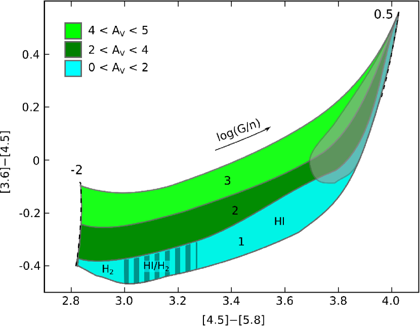
Figure 1.— IRAC [${3.6}$]–[${4.5}$] vs. [${4.5}$]–[${5.8}$] color-color plot indicating the region occupied by PDRs (PAH grains and UV fluorescent H₂). Region 1 of color-color space is occupied by gas clouds of thickness $A_{V}\sim$ 0–2 mag. Region 2 of color-color space is occupied by either a gas cloud of thickness $A_{V}\sim$ 2–4 mag in front of the incident UV source or a gas cloud ($A_{V}>2$) behind the incident UV source. Region 3 indicate a cloud thickness $A_{V}\sim$ 4–5 mag in front of the incident FUV source. The grey region at [${4.5}$]–[${5.8}$] $>$ 3.6 indicates region of color space with significant degeneracy.

There is often degeneracy for physical parameters of emitting material in color space, thus the usefulness of color space analysis in extracting information is restricted to regions in color space that reveals breaks in degeneracy. From our investigation of the calculated IRAC colors, we find that the [${3.6}$]–[${4.5}$] vs. [${4.5}$]–[${5.8}$] color space in the region where 2.9 $<$ [${4.5}$]–[${5.8}$] $<$ 3.6 has minimal degeneracy and is useful as a tool for analysis. We divide this region into 3 sub-regions. Figure 1 shows the IRAC [${3.6}$]–[${4.5}$] vs. [${4.5}$]–[${5.8}$] color-color plot indicating these various regions.

Region 1.— This region of color space is defined by a lower limit

[$${3.6} {4.5} >0.15(\mbox{[${4.5}$]--[${5.8}$]})-0.92$$]–[]

for $$3.0<\mbox{[${4.5}$]--[${5.8}$]}<3.2$$

[$${3.6} {4.5} >0.35(\mbox{[${4.5}$]--[${5.8}$]})-1.56$$]–[]

for $$3.2<\mbox{[${4.5}$]--[${5.8}$]}<3.6$$

and upper limit

[$${3.6} {4.5} <0.27(\mbox{[${4.5}$]--[${5.8}$]})-1.19$$]–[]

for $$3.0<\mbox{[${4.5}$]--[${5.8}$]}<3.3$$

[$${3.6} {4.5} <0.50(\mbox{[${4.5}$]--[${5.8}$]})-1.95$$]–[]

for $$3.3<\mbox{[${4.5}$]--[${5.8}$]}<3.6.$$

This region of color space is mostly occupied by thin PDRs of thickness $A_{V}\sim$ 0 to 2 mag. The colors from a plane-parallel PDR model would be found in this region of color space.

Region 2.— This region of color space is defined by an upper limit of

[$${3.6} {4.5} <0.35(\mbox{[${4.5}$]--[${5.8}$]})-1.31$$]–[]

for $$3.0<\mbox{[${4.5}$]--[${5.8}$]}<3.6.$$

This region of color space is occupied by two cases of PDRs: a) A gas cloud of thickness $A_{V}\sim\mbox{2--4}$ mag in front of the incident FUV source, or b) A thick gas cloud behind the incident FUV source. For a thick cloud behind the FUV source, material beyond $A_{V}>2$ mag does not significantly contribute to the total line of sight emission. Additionally the line of sight emission will begin to include a contribution from fluorescent H₂ lines.

Region 3.— This region of color space is defined by an upper limit of

[$${3.6} {4.5} <0.20(\mbox{[${4.5}$]--[${5.8}$]})-0.72$$]–[]

for $$3.0<\mbox{[${4.5}$]--[${5.8}$]}<3.4$$

[$${3.6} {4.5} <0.70(\mbox{[${4.5}$]--[${5.8}$]})-2.42$$]–[]

for $$3.4<\mbox{[${4.5}$]--[${5.8}$]}<3.6.$$

Incident UV source is behind a gas cloud of thickness $A_{V}\sim\mbox{4--5}$. The increasing [${3.6}$]–[${4.5}$] color partly due to the increasing contribution of UV fluorescent H₂ emission in the line of sight spectra.

Another result of our calculation is that the [${4.5}$]–[${5.8}$] color is an approximate indicator of the $G/n_{\rm{H}}$ ratio where the line of sight intersects the plane of the incident FUV. We fit the following analytic form to this relationship:

$$\log(G/n_{\rm{H}})=-19.7+10.0a-1.35a^{2},$$

where $a=\mbox{[${4.5}$]--[${5.8}$]}$ and $2.8<a<3.8$. This relationship is due in part to the dependence of the ionization fraction on $G/n_{\rm{H}}$. Larger $G/n_{\rm{H}}$ results in larger overall ionization fraction of the PAHs and thus the increase PAH feature (5.270, 5.700, 6.220 $\mu$m) emission in the 5.8 $\mu$m band relative to the continuum emission in the 4.5 $\mu$m band. Our simple model does not take into account PAH destruction from strong FUV fields which could effect this color relationship. At $G/\mbox{$n_{\mathrm{H}}$}\lesssim 0.04$, H₂ begins forming due to self-shielding, and thus the 4.5 $\mu$m band will also include emission from UV fluorescent H₂ lines (Hollenbach & Tielens, 1999).

Finally, we find that the [${4.5}$]–[${5.8}$] color can be used to probe the phase of the gas (molecular, mixed, or atomic) where the line of sight intersects the plane of the incident FUV. The emission of gas within the H I/H₂ transition zone will have a [${4.5}$]–[${5.8}$] color within the range 3.0–3.3. Mostly molecular gas ($n({\rm{H_{2}}})/n_{\rm{H}}>0.3$) will have [${4.5}$]–[${5.8}$] $<$ 3.0 and mostly atomic gas ($n({\rm{H_{2}}})/n_{\rm{H}}<0.25$) will have [${4.5}$]–[${5.8}$] $>$ 3.3 (see Fig. 1). Our calculations show that within the H I/H₂ transition zone the contribution of H₂ ro-vibrational lines to total emission is $\sim$ 5-10% in the 3.6 $\mu$m band and $\sim$ 10-20% in the 4.5 $\mu$m band. Our model did not include the possible freeze out of small PAH molecules in cold molecular gas ($\log(G/\mbox{$n_{\mathrm{H}}$})\lesssim-2$) which would reduce the contribution of PAH emission in the IRAC bands.

It should be noted that external foreground extinction can affect the IRAC colors, although this effect is not very strong due to the relative flatness of the MIR extinction curve (Lutz et al., 1996). Application of most MIR extinction laws result in the [${4.5}$]–[${5.8}$] color to be negligibly effected by extinction (Lutz, 1999; Indebetouw et al., 2005). The [${3.6}$]–[${4.5}$] color appears to have a stronger dependence on extinction, however, an $A_{V}$ = 10 mag extinction only results in an increase in the [${3.6}$]–[${4.5}$] color of $\sim$ 0.1 (Indebetouw et al., 2005; Chapman et al., 2009). However, due to variations of the MIR extinction law with environment, the effect of extinction on the [${3.6}$]–[${4.5}$] color may be even less (Wang et al., 2013).

3.2. Distinguishing between shocked and UV fluorescent molecular hydrogen

It is often the case that the excitation mechanism for H₂ emission is unknown, and in some cases is necessary to understand the nature of the emission. For example the H₂ emission from externally illuminated structures such as pillars or globulettes can have a similar morphology to bow shocks from protostellar outflows. We propose the following simple one-color diagnostic that should suffice in most cases of interest where H₂ has already been detected (e.g., NIR H₂ 2.12 $\mu$m imaging):

Shocked: $$\mbox{[${3.6}$]--[${4.5}$]}\geq 0.5$$

UV Flourescent: $$\mbox{[${3.6}$]--[${4.5}$]}<0.5$$

This diagnostic is particularly useful when only data from the first two IRAC channels are available, such as data from the Spitzer Warm Mission. For analysis including the 5.8 $\mu$m band, the region of color space defined for shocked H₂ emission is

[$${3.6} {4.5} >-0.24\mbox{[${4.5}$]--[${5.8}$]}+1.26$$]–[]

for $$0.25<\mbox{[${4.5}$]--[${5.8}$]}<1.5$$

[$${3.6} {4.5} >0.8\mbox{[${4.5}$]--[${5.8}$]}+1.0$$]–[]

for $$-0.5<\mbox{[${4.5}$]--[${5.8}$]}\leq 0.25$$

(Ybarra et al., 2010), whereas, gas containing UV fluorescent H₂ will be in the PDR color space defined in section 3.1. Figure 2 shows a larger color-color map showing the location of shocked H₂ emission in relation to UV excited PDR emission.

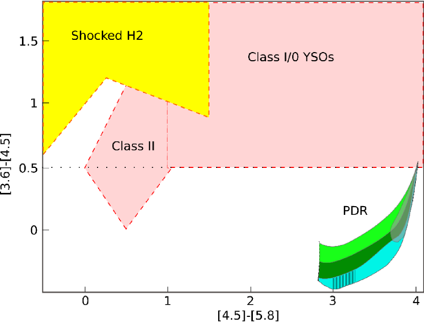
Figure 2.— Spitzer IRAC [${3.6}$]–[${4.5}$] vs. [${4.5}$]–[${5.8}$] color-color plot showing the location of shocked H₂ emission in relation to UV excited PDR emission.

3.3. Background Estimation Method

In order to measure the emission in each pixel it is necessary to model the background. For small scale structures, such as shocked H₂ knots against a variable background, a ring filter can be used to effectively model the background (Ybarra & Lada, 2009). However, for the analysis of more extended emission, such as that from PDRs, we use a Bayesian intensity estimator developed by Bijaoui (1980). The pixel intensity histogram is modeled with a Gaussian distribution for noise centered near the sky background level and an exponential distribution prior to describe the asymmetry of the histogram due to non-background emission. The model has the following analytic form:

$$p(I)=\frac{1}{2a}\exp(\mbox{\raisebox{1.29167pt}{${\sigma^{2}\!}$}/\raisebox{-0.86108pt}{${2a^{2}}$} })\exp[-(I-s)/a]\mbox{erfc}\left(\frac{\alpha}{\sqrt{2}}\right),$$

where

$$\alpha=\frac{\sigma}{a}-\frac{(I-s)}{\sigma},$$

$I$ is the measured pixel intensity, $s$ is the background level, $\sigma$ is the width of the Gaussian, and $a$ is the scale parameter of the exponential distribution. We fit the function $p(I)$ to the intensity histogram to obtain the values $a$, $\sigma$, and $s$. The Bayesian estimator of the true intensity is

$$\hat{i}=I-s-\frac{\sigma^{2}}{a}+\sqrt{\frac{2}{\pi}}\frac{\sigma e^{-\alpha^{2}/2}}{\mbox{erfc}(\mbox{\raisebox{1.29167pt}{${\alpha}$}/\raisebox{-0.86108pt}{${\!\sqrt{2}}$} })}.$$

Therefore for every pixel in the image we are able to estimate the intensity above the background, and subsequently with the registered images we are able to calculate the color for each pixel.

4. Application of the Method: NGC 2316

The usefulness of any method needs to be tested. We apply this method to archival Spitzer IRAC images of the NGC 2316 (=Parsamyan 18 =L1654, ($\alpha$,$\delta$)(J2000) = $6^{\mathrm{h}}59^{\mathrm{m}}40^{\mathrm{s}}$, $-7\arcdeg 46\arcmin 36\arcsec$) from program 3290 (PI: Langer) (catalog ADS/Sa.Spitzer#10707712). This region is a site of star formation containing a young (2–3 Myr) embedded cluster with line of sight extinction $\langle A_{V}\rangle$ = 4.5 mag at a distance of 1.1 kpc(Teixeira et al., 2004). Within this region exists a PDR generated by the FUV radiation from a ZAMS B3 star (López et al., 1988; Ryder et al., 1998).

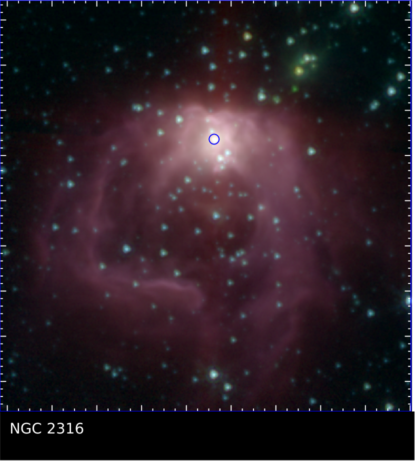
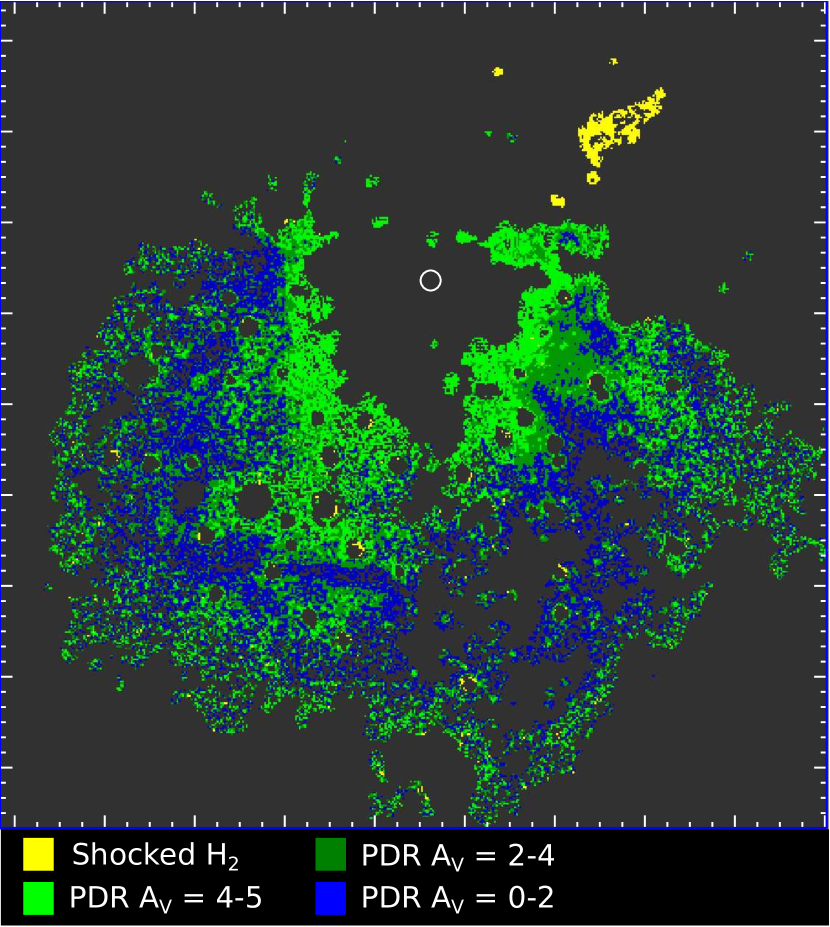
Figure 3.— a) Spitzer IRAC 3-color (R: 5.8 $\mu$m, G: 4.5 $\mu$m, B: 3.6 $\mu$m) image of NGC 2316. Image is centered at ($\alpha$,$\delta$)(J2000) = (6^h59^m42$\fs$0, $-$7°47′11″) with a FOV of 4.54′$\times$ 4.54′. The small circle indicates the location of the B3 star. b) Map of identified emission from color analysis. Yellow indicate pixels whose IRAC colors are consistent with that of shocked H₂ emission. Blue, dark green, and light green indicate pixels with IRAC colors consistent with PDRs with line of sight thicknesses of $A_{V}\sim$ 0–2 mag, 2–4 mag, and 4–5 mag, respectively.

Figure 3a shows a Spitzer IRAC 3-color image of the cluster. Figure 3b shows a map of the results from our color analysis. The color-coded yellow regions indicate pixels whose IRAC colors are consistent with that of shocked H₂ emission. Blue, dark green, and light green indicate pixels with IRAC colors consistent with PDRs with line of sight thicknesses of $A_{V}\sim$ 0–2 mag, 2–4 mag, and 4–5 mag, respectively.

We find the emission around the B3 star to have colors consistent with PDRs with line of sight thickness of $A_{V}>4$ mag. We are able deduce that this PDR results from an exciting source embedded within the cloud. which is consistent with previous studies of the region (Ryder et al., 1998; Velusamy & Langer, 2008) Our analysis is also consistent with the results from the NIR H₂ study by Ryder et al. (1998). We identify five of the eight H₂ emission regions in our color analysis (R2=North Peak, R4=S Peak, R6=NW Arc, R7=W Arc, R8=P 18 NW).

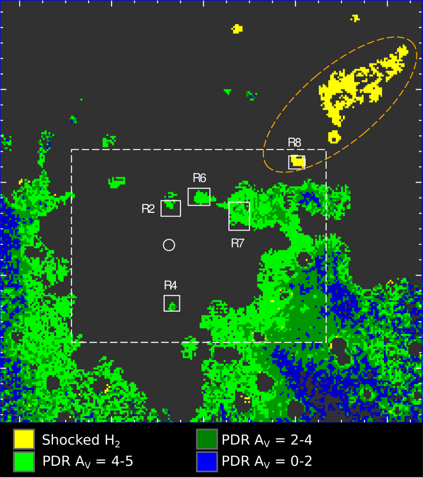
Figure 4.— Map of identified emission from color analysis. The solid boxes indicate the locations of five of the H₂ emission regions studied by Ryder et al. (1998). The dashed box indicates FOV of the Ryder et al. (1998) H₂ study. The orange ellipse indicates the proposed outflow. The circle represents the location of the B3 star. The map is centered at ($\alpha$,$\delta$)(J2000) = (6^h59^m40$\fs$7, $-$7°46′17″) with a FOV of 2.27^′ $\times$ 2.27^′.

Figure 4 shows a color analysis map with the locations of the five emission regions indicated by solid boxes. Four of these regions (R2, R4, R6, R7) were found by Ryder et al. (1998) to have H₂ emission excited through UV fluorescence. These four regions are part of the H₂ shell observed by Velusamy & Langer (2008). Our color analysis of these four regions reveals they have colors consistent with PDR emission from a cloud with thickness $A_{V}\sim$ 4–5 mag. Additionally, those four regions have $\mbox{[${3.6}$]--[${4.5}$]}\sim$ 3.2–3.3, corresponding to the H I/H₂ transition zone where H₂ is expected to strongly emit (Hollenbach & Tielens, 1999).

Ryder et al. (1998) found that the region R8 has a H₂ (1–0)/(2–1) S(1) line ratio consistent with shock excitation and therefore suggest R8 may be part of an outflow possibly associated with the previously observed CO outflow found in the region (Fukui et al., 1993). Our analysis reveals this region to have IRAC colors consistent with shock excited H₂ and therefore confirming the previous result. Northwest of R8 our color analysis reveals more emission that may be shock excited This emission has an elongated structure that along with R8 may be part of an outflow originating from the B3 star or a nearby neighbor. The projected length of this structure is 0.27 pc (51″) and the projected distance from the B3 star to the furthest edge is 0.53 pc (99″).

5. Conclusions

We created a set of Spitzer IRAC color diagnostics to study the extended MIR emission observed in star forming regions. For PDRs, color diagnostics allow one to probe the depth of the region, the phase of the gas, and estimate the ratio of FUV to gas density. Additionally, we show that color analysis can distinguish between FUV excited and shock excited H₂ emission. We present a one-color diagnostic that is able to make use of new data from the Spitzer Warm Mission for distinguishing the excitation processes. To demonstrate the usefulness of our method we applied it to Spitzer IRAC observations of NGC 2316 and find our results are consistent with previous studies of the nebula. Additionally we identify shocked gas which may be part of an outflow originating from the cluster.

References

- Bijaoui (1980) Bijaoui, A. 1980, A&A, 84, 81
- Black & Dalgarno (1976) Black, J. H., & Dalgarno, A. 1976, ApJ, 203, 132
- Black & van Dishoeck (1987) Black, J. H., & van Dishoeck, E. F. 1987, ApJ, 322, 412
- Butler & Tan (2009) Butler, M. J., & Tan, J. C. 2009, ApJ, 696, 484
- Chapman et al. (2009) Chapman, N. L., Mundy, L. G., Lai, S.-P., & Evans, II, N. J. 2009, ApJ, 690, 496
- Cyganowski et al. (2009) Cyganowski, C. J., Brogan, C. L., Hunter, T. R., & Churchwell, E. 2009, ApJ, 702, 1615
- Draine (1978) Draine, B. T. 1978, ApJS, 36, 595
- Draine & Li (2007) Draine, B. T., & Li, A. 2007, ApJ, 657, 810
- Ferland et al. (2013) Ferland, G. J., Porter, R. L., van Hoof, P. A. M., et al. 2013, Rev. Mexicana Astron. Astrofis., 49, 137
- Fukui et al. (1993) Fukui, Y., Iwata, T., Mizuno, A., Bally, J., & Lane, A. P. 1993, in Protostars and Planets III, ed. E. H. Levy & J. I. Lunine, 603–639
- Giannini et al. (2013) Giannini, T., Lorenzetti, D., De Luca, M., et al. 2013, ApJ, 767, 147
- Gutermuth et al. (2008) Gutermuth, R. A., Myers, P. C., Megeath, S. T., et al. 2008, ApJ, 674, 336
- Hollenbach & Tielens (1999) Hollenbach, D. J., & Tielens, A. G. G. M. 1999, Reviews of Modern Physics, 71, 173
- Hora et al. (2008) Hora, J. L., Carey, S., Surace, J., Marengo, M., et al. 2008, PASP, 120, 1233
- Indebetouw et al. (2005) Indebetouw, R., Mathis, J. S., Babler, B. L., et al. 2005, ApJ, 619, 931
- López et al. (1988) López, J. A., Roth, M., Friedman, S. D., & Rodríguez, L. F. 1988, Rev. Mexicana Astron. Astrofis., 16, 99
- Lutz et al. (1996) Lutz, D., Feuchtgruber, H., Genzel, R., et al. 1996, A&A, 315, L269
- Lutz (1999) Lutz, D. 1999, The Universe as Seen by ISO, 427, 623
- Noriega-Crespo et al. (2004) Noriega-Crespo, A., Morris, P., Marleau, F. R., et al. 2004, ApJS, 154, 352
- Rathborne et al. (2006) Rathborne, J. M., Jackson, J. M., & Simon, R. 2006, ApJ, 641, 389
- Reach et al. (2005) Reach, W. T., Megeath, S. T., Cohen, M., Hora, J., et al. 2005, PASP, 117, 978
- Ryder et al. (1998) Ryder, S. D., Allen, L. E., Burton, M. G., Ashley, M. C. B., & Storey, J. W. V. 1998, MNRAS, 294, 338
- Shaw et al. (2005) Shaw, G., Ferland, G. J., Abel, N. P., Stancil, P. C., & van Hoof, P. A. M. 2005, ApJ, 624, 794
- Simpson et al. (2012) Simpson, R. J., Povich, M. S., Kendrew, S., et al. 2012, MNRAS, 424, 2442
- Teixeira et al. (2004) Teixeira, P. S., Fernandes, S. R., Alves, J. F., et al. 2004, A&A, 413, L1
- van Hoof et al. (2004) van Hoof, P. A. M., Weingartner, J. C., Martin, P. G., Volk, K., & Ferland, G. J. 2004, MNRAS, 350, 1330
- Velusamy & Langer (2008) Velusamy, T., & Langer, W. D. 2008, AJ, 136, 602
- Velusamy et al. (2014) Velusamy, T., Langer, W. D., & Thompson, T. 2014, ApJ, 783, 6
- Wang et al. (2013) Wang, S., Gao, J., Jiang, B. W., Li, A., & Chen, Y. 2013, ApJ, 773, 30
- Weingartner & Draine (2001) Weingartner, J. C., & Draine, B. T. 2001, ApJ, 548, 296
- Ybarra & Lada (2009) Ybarra, J. E., & Lada, E. A. 2009, ApJ, 695, L120
- Ybarra et al. (2010) Ybarra, J. E., Lada, E. A., Balog, Z., Fleming, S. W., & Phelps, R. L. 2010, ApJ, 714, 469