Thermal Phase Transitions of Strongly Correlated Bosons with Spin-Orbit Coupling

Abstract

Experiments on ultracold atoms have started to explore lattice effects and thermal fluctuations for two-component bosons with spin-orbit coupling (SOC). Motivated by this, we derive and study a $tJ$ model for lattice bosons with equal Rashba-Dresselhaus spin-orbit coupling (SOC) and strong Hubbard repulsion in a uniform Zeeman magnetic field. Using the Gutzwiller ansatz, we find strongly correlated ground states with stripe superfluid (SF) order. We formulate a finite temperature generalization of the Gutzwiller method, and show that thermal fluctuations in the doped Mott insulator drive a two-step melting of the stripe SF, revealing a wide regime of a stripe normal fluid.

Spin orbit coupling (SOC) underlies a diverse range of remarkable phases in solid state materials including topological insulators Hasan and Kane (2010); Qi and Zhang (2011), quantum anomalous Hall insulators Haldane (1988); Chang et al. (2013), and Skyrmion crystals Yu et al. (2010), while its interplay with strong correlations is expected to lead to exotic topological Mott insulators Pesin and Balents (2010); Witczak-Krempa et al. (2014). Experiments on ultracold atomic gases have started to explore analogous issues for SOC in Bose fluids, using Raman transitions to induce an equal Rashba-Dresselhaus SOC and a uniform Zeeman magnetic field Lin et al. (2011); Zhang et al. (2012); Dalibard et al. (2011); LeBlanc et al. (2013); Qu et al. (2013); Beeler et al. (2013); Ji et al. (2014); Hamner et al. (2014); Fu et al. (2014). Striking observations include the spin Hall effect Beeler et al. (2013) and tunable production of Feshbach molecules Fu et al. (2014). On the theoretical front, Bose superfluids with equal Rashba-Dressehaus coupling have been shown to exhibit stripe orders, and spin and density coupled collective modes Stanescu et al. (2008); Wang et al. (2010); Ho and Zhang (2011); Radić et al. (2011); Li et al. (2012); Martone et al. (2012); Chen and Zhai (2012); Li et al. (2013); Lü and Sheehy (2013). Pure Rashba SOC, with a circular minimum in the single particle dispersion, may lead to unusual fluctuation effects Jian and Zhai (2011); Ozawa and Baym (2012a); Barnett et al. (2012); Ozawa and Baym (2012b); Anderson et al. (2013), ferromagnetism Riedl et al. (2013), or topological ground states Sedrakyan et al. (2012); Ramachandhran et al. (2013). Incorporating strong correlations on a lattice induces superfluids or Mott insulators with remarkable spin textures Graß et al. (2011); Mandal et al. (2012); Cole et al. (2012); Radić et al. (2012); Cai et al. (2012b); Xu et al. (2014); Qian et al. (2013); Sun et al. (2014); He et al. (2014) and topological transport properties Wong and Duine (2013). Very recently, experiments have started to explore thermal phase transitions Ji et al. (2014), and the effects of a periodic lattice potential Hamner et al. (2014), in a Bose-Einstein condensate (BEC) with equal Rashba-Dresselhaus SOC.

Motivated by the broad interest in understanding the interplay of SOC and strong correlations, and ongoing experimental efforts in ultracold gases, we focus here on two important questions. (a) How does the presence of a lattice and strong correlations modify the ground states of bosons with equal Rashba-Dresselhaus SOC? (b) How do thermal fluctuations impact Bose superfluids with SOC? Our key results are the following. (i) At strong correlations, we derive an effective $tJ$ model for lattice bosons with equal Rashba-Dresselhaus SOC and a uniform magnetic field. Using a zero temperature Gutzwiller ansatz, we show that this leads to strongly correlated variants of stripe and incommensurate SFs previously discussed in the continuum. However, unlike in the continuum, applying a large magnetic field leads to three distinct SFs (see Fig. 1(a,b)) depending on the SOC angle: (a) a zero momentum SF analogous to the continuum case, (b) a $\pi$-momentum SF, or (c) a $\pi/2$-momentum SF. (ii) At weaker field, strong interactions induce stripe order; in contrast to the continuum, the stripe order has significant higher harmonic content resulting in extra peaks in the momentum distribution as seen from Fig. 1(c,d). (iii) Previous work has considered thermal fluctuations of weakly interacting continuum bosons with SOC Jian and Zhai (2011); Ozawa and Baym (2012a). Here, to study strongly interacting lattice bosons, we formulate a stochastic Gutzwiller approach, which treats strong quantum correlations at mean field level, but retains full knowledge of spatial thermal fluctuations. The Monte Carlo (MC) technique introduced here is of broad applicability, being especially useful when the sign problem prevents quantum MC simulations, such as for frustrated bosons. (iv) Using this approach, we obtain the concrete temperature-doping phase diagram of spinor lattice bosons with SOC and strong correlations as shown in Fig. 2. Thermal fluctuations are shown to destroy superfluidity well below the stripe transition, leading to a wide window of a normal Bose fluid with stripe order, this regime being enhanced near the Mott insulator.

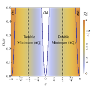
(a)

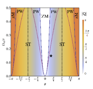
(b)

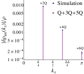
(c)

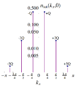
(d)

Figure 1: (a) Magnetic field ($\Omega_{R}$) evolution of the dispersion for noninteracting bosons, with double minima at $(\pm Q,0)$ for SOC angle $\theta$. At large $\Omega_{R}$, we find a unique minimum at $Q=0$ (i.e., $ZM$) or $Q=\pi$ (i.e., $\pi$M). At $\theta=\pm\pi/2$, minima are pinned to $(\pm\pi/2,0)$. (b) Interacting $T=0$ phase diagram at density $\rho=0.5$, showing emergent plane wave ($PW$) and stripe ($ST$) states at $U/t=10$ and $\lambda=0.95$. $\star$ is the point at which we plot (c) density modulation, and (d) momentum distribution, comparing simulations (dots) and the variational ansatz (line) with three harmonics.

Noninteracting lattice Hamiltonian. — We work on a square optical lattice with lattice spacing $d$, and consider the hopping Hamiltonian for two-component bosons,

$$\!\!\!\!H_{\rm kin}\!=\!-t\!\sum_{\langle ij\rangle}(b_{i\alpha}^{\dagger}R_{\alpha\beta}^{i,j}b^{\phantom{\dagger}}_{j\beta}+h.c.)-\frac{\Omega_{R}}{2}\!\sum_{i}\left(n_{i\uparrow}\!-\!n_{i\downarrow}\right).$$ (1)

Here, $R^{i,i+\hat{y}}=\mathbb{I}$, $R^{i,i+\hat{x}}=e^{i\theta\sigma_{y}}$, and the SOC angle $\theta$ dictates the ratio of spin-flip to spin-conserving hopping amplitudes. For long wavelength modes, with momenta $k\ll 1/d$, this Hamiltonian reduces to

$$H^{\rm long}_{\rm kin}({{\bf{k}}})\approx b^{\dagger}_{{{\bf{k}}}\alpha}\left[\frac{k_{\ell}^{2}}{2m_{\ell}}\delta^{\alpha\beta}+\gamma k_{x}\sigma^{\alpha\beta}_{y}-\frac{\Omega_{R}}{2}\sigma^{\alpha\beta}_{z}\right]b^{\phantom{\dagger}}_{{{\bf{k}}}\beta},$$ (2)

where $\ell=x,y$ with an implicit sum over $\ell$. This is the form of the experimentally realized continuum Hamiltonian (at zero detuning). We identify the equal Rashba-Dresselhaus SOC coupling $\gamma=2td\sin\theta$, anisotropic inverse effective masses, $m^{-1}_{x}\!=\!2td^{2}\cos\theta$ and $m^{-1}_{y}\!=\!2td^{2}$, induced by the lattice, and a Raman laser induced Zeeman field $\Omega_{R}$. (Henceforth, we set $d=1$.) For general ${{\bf{k}}}$, we find mode energies on the lattice

$$\!\!E^{\pm}_{{\bf{k}}}\!=\!-2t\left(\cos\!\theta\!\cos\!k_{x}\!+\!\cos\!k_{y}\right)\!\pm\!\sqrt{\frac{\Omega_{R}^{2}}{4}\!+\!4t^{2}\!\sin^{2}\!\theta\sin^{2}\!k_{x}}.$$

Focusing on the lower branch, $E^{-}_{{\bf{k}}}$, the dispersion exhibits degenerate minima at $(k_{x},k_{y})=(\pm Q,0)$, similar to the continuum. At $\Omega_{R}\!=\!0$, we get $Q\!=\!\theta$.

For $\Omega_{R}\neq 0$, we find three regimes. (i) $-\pi/2\!<\!\theta\!<\!\pi/2$: Increasing $\Omega_{R}$ leads to $Q\!\to\!0$, and we eventually lock into $Q=0$ for $\Omega_{R}>\Omega^{c}_{R}\equiv 4t|\sin\theta\tan\theta|$; this regime is labelled zero-momentum (ZM). (ii) $\pi/2\!<\!|\theta|\!<\!\pi$: The minima shift in the opposite direction with increasing field, locking into $Q\!=\!\pi$ for $\Omega_{R}>\Omega^{c}_{R}$, a regime we label $\pi$-momentum ($\pi$M). A similar $\pi$M state, but with $k_{y}=\pm\pi$, is found for bosons with Rashba SOC in a 1D spin-dependent periodic potential along the $x$-direction Han2012 , which acts as a staggered magnetic field. (iii) $\theta\!=\!\pm\pi/2$: Here an extra symmetry appears, namely, ${\cal U}^{\dagger}H_{\rm kin}{\cal U}\!=\!H_{\rm kin}$, where the unitary operator ${\cal U}$ acts as ${\cal U}^{\dagger}b^{\phantom{\dagger}}_{i\alpha}{\cal U}\!=\!b^{\phantom{\dagger}}_{{\cal M}_{i}\alpha}(-1)^{x_{i}}$, with the site ${\cal M}_{i}\!\equiv\!(-x_{i},y_{i})$ obtained by reflection about the $y$-axis. In momentum space, this sends $k_{x}\!\to\!-k_{x}\!+\!\pi$, which maps the minimum back onto itself, pinning $Q$ to $\pm\pi/2$ for any $\Omega_{R}$. The strong field limit on the lattice thus leads to richer possibilities than the continuum Stanescu et al. (2008); Wang et al. (2010); Ho and Zhang (2011); Radić et al. (2011); Li et al. (2012); Martone et al. (2012); Chen and Zhai (2012); Li et al. (2013); Lü and Sheehy (2013). Fig. 1(a) depicts the dispersion as a function of $\Omega_{R}/t$ and $\theta$, tracking the evolution of $Q$, and marking boundaries where we reach $Q=0,\pi$. A degenerate “double well” in the dispersion at $(\pm Q,0)$ leads to a macroscopic degeneracy of many-body ground states for noninteracting bosons. We next study how strong correlation effects break this degeneracy.

Strongly interacting regime. — The hopping Hamiltonian in Eq. 1 is in the conventional gauge choice where the atomic hyperfine states are eigenstates of $\sigma_{y}$. Labelling hyperfine flavors by $c,d$, the local Hubbard interaction $H_{\rm U}=U_{cc}n_{c}(n_{c}-1)/2+U_{dd}n_{d}(n_{d}-1)/2+U_{cd}n_{c}n_{d}$. We choose $U_{cc}=U_{dd}=U$ and set $U_{cd}=\lambda U$ ($\lambda<1$ for ⁸⁷Rb). For $U\gg t$, double occupancy of bosons leads to a large energy cost. For fillings $\rho\leq 1$ boson per site, we thus use perturbation theory in $t/U$ Cole et al. (2012); Radić et al. (2012); Cai et al. (2012b) to derive an effective Hamiltonian in the restricted Hilbert space where double occupancies are forbidden (see Supplemental Material SuppMat for derivation). The resulting effective strong coupling Hamiltonian is given by

$$H_{\rm eff}={\cal P}H_{\rm kin}{\cal P}\!+\!\sum_{i\delta}J_{\delta}^{a}S_{i}^{a}S_{i+\delta}^{a}+\sum_{i\delta}\mathbf{D}^{\phantom{\dagger}}_{\delta}\cdot(\mathbf{S}^{\phantom{\dagger}}_{i}\times\mathbf{S}^{\phantom{\dagger}}_{i+\delta})$$ (3)

with $\delta=\hat{x},\hat{y}$. The first term denotes the kinetic energy term in Eq. 1 (including the magnetic field $\Omega_{R}$) projected to the Hilbert space of no double occupancy, with ${\cal P}$ being the Gutzwiller projection operator. The next two terms describe exchange interactions, with the spin operator $\mathbf{S}^{a}_{i}=\frac{1}{2}b^{\dagger}_{i\alpha}\sigma^{a}_{\alpha\beta}b^{\phantom{\dagger}}_{i\beta}$, and the exchange coefficients $J^{a}_{\delta}$ and Dzyaloshinskii-Moriya vectors $\mathbf{D}_{\delta}$ listed Table 1.

Zero temperature phase diagram. — The Gutzwiller ansatz provides a powerful approach to strongly correlated bosons Gutzwiller (1963); Krauth et al. (1992). This variational wavefunction is constructed as a direct product (over all sites) of single-site wavefunctions, with each single-site wavefunction being capable of describing states with fluctuating or fixed particle number, thus providing a mean field description of a superfluid or a Mott insulator ground state. For two-component bosons Cole et al. (2012) the ansatz including the spin degree of freedom and no double occupancy constraint is

$$\ket{\Psi}=\overset{N}{\underset{i=1}{\otimes}}(\chi_{i0}\ket{0}+\chi_{i\uparrow}\ket{\uparrow}+\chi_{i\downarrow}\ket{\downarrow})$$ (4)

where $\chi_{in}$ are complex variational parameters, with normalization fixing $\sum_{n}\left|\chi_{i,n}\right|^{2}=1$ at each site $i$ (with $n=0,\uparrow,\downarrow$). Minimizing $\langle\Psi|H_{\rm eff}|\Psi\rangle$ by optimizing $\{\chi_{in}\}$ yields the phase diagram shown in Fig. 1(b).

We highlight three key differences between the lattice phase diagram and its continuum counterpart. (i) The single-particle dispersion has two degenerate minima at ${{\bf{k}}}=(\pm Q,0)$; this leads to a macroscopic many-body ground state degeneracy for noninteracting bosons, since they can condense into any arbitrary superposition of wavefunctions constructed from these minima. Interactions split this degeneracy resulting in two phases for $\lambda<1$: a Stripe ($ST$) state featuring an equal superposition of the two minima, and a Plane Wave ($PW$) featuring condensation into a single minimum. However, the lattice features two distinct $ST$ and $PW$ phases, with momentum distribution peaks evolving with $\Omega_{R}$ to be closer to $ZM$ or $\pi M$. In addition, the wavevector of the $ST$ state at $\theta\!=\!\pm\pi/2$ is pinned to $Q=\pm\pi/2$ at all $\Omega_{R}$, since interactions preserve the previously discussed symmetry, so that ${\cal U}^{\dagger}H_{\rm eff}{\cal U}=H_{\rm eff}$. (ii) Strong correlations suppress $\Omega_{R}^{c}$ by a factor $\!\sim\!(1\!-\!\rho)$, leading to an enlarged window of $ZM$/$\pi M$ (see Fig. 1(a,b)). (iii) The continuum $ST$ state has a density modulation with a dominant harmonic amplitude $\delta\rho(2Q)\!\sim\!m_{z}$, where $m_{z}$ is the uniform magnetization induced by $\Omega_{R}$ Li et al. (2012). By contrast, the lattice $ST$ state has strong mode-mode coupling, lead to higher order Fourier peaks in the density and momentum distribution; see Fig. 1(c,d). This suppresses the real space density modulation by an order of magnitude, while still allowing for significant $m_{z}$.

Table 1: Exchange couplings along the $\hat{x},\hat{y}$ directions in the strong coupling bosonic $tJ$ Hamiltonian in Eq.3

$J^{x}_{\hat{x}}=-\frac{4t^{2}}{\lambda U}\cos 2\theta$	$J^{x}_{\hat{y}}=-\frac{4t^{2}}{\lambda U}$
$J^{y}_{\hat{x}}=-\frac{4t^{2}}{\lambda U}(2\lambda-1)$	$J^{y}_{\hat{y}}=-\frac{4t^{2}}{\lambda U}(2\lambda-1)$
$J^{z}_{\hat{x}}=-\frac{4t^{2}}{\lambda U}\cos 2\theta$	$J^{z}_{\hat{y}}=-\frac{4t^{2}}{\lambda U}$
$\mathbf{D}_{\hat{x}}=-\frac{4t^{2}}{\lambda U}\sin 2\theta\,\hat{y}$	$\mathbf{D}_{\hat{y}}=0$

The various phases we find from our numerical minimization are reasonably captured by a variational ansatz

$$\!\!\!\begin{pmatrix}\chi_{i\uparrow}\\ \chi_{i\downarrow}\end{pmatrix}\!\!=\!\!\!\!\!\sum_{n={\rm odd}}\!\!\left[\!\frac{c_{n}}{\sqrt{2}}\begin{pmatrix}\!a_{n}\!\\ \!b_{n}\!\end{pmatrix}\!e^{iQnx_{i}}\!+\!\frac{c_{-n}}{\sqrt{2}}\begin{pmatrix}\!a_{n}\!\\ \!-b_{n}\!\end{pmatrix}\!e^{-iQnx_{i}}\!\right]$$ (5)

where $a_{n}\!=\!\sin\phi_{n}\!+\!\cos\phi_{n}$, $b_{n}\!=\!i(\sin\phi_{n}\!-\!\cos\phi_{n})$, the sum is over odd integers $n\!>\!0$, and $\chi_{i0}\!=\!(1\!-\!\left|\chi_{i\uparrow}\right|^{2}\!-\!\left|\chi_{i\downarrow}\right|^{2})^{1/2}$. Retaining the leading term ($n\!=\!1$) reveals three states: $(i)$ Stripe ($ST$) order with $c_{1}=c^{*}_{-1}=\sqrt{\rho/2}$, representing an equal superposition of modes at $(\pm Q,0)$, $(ii)$ Plane Wave ($PW$) order with $\{c_{1},c_{-1}\}=\{0,\sqrt{\rho}\}$ or $\{\sqrt{\rho},0\}$ representing a single mode condensate at $(\pm Q,0)$, and $(iii)$ a $ZM/\pi M$ state with spins fully polarized along the $\Omega_{R}$-axis. Limiting to $n\!=\!1,3,5$ quantitatively captures the leading harmonics in the density and momentum distribution in Fig. 1(c,d), but leads to a 20% error in the highest harmonic resolved in our simulations.

A strong coupling perspective is afforded by the local gauge transformation, $b_{i}=\left(b_{i\uparrow},b_{i\downarrow}\right)^{T}\rightarrow e^{-i\theta x_{i}\sigma_{y}}\tilde{b}_{i}$, which leads to

$$\tilde{H}_{\rm eff}= -t\sum_{\left<ij\right>}\left(\tilde{b}_{i\alpha}^{\dagger}\tilde{b}_{j\alpha}+h.c.\right)+\sum_{\langle ij\rangle}\tilde{J}^{\alpha}\tilde{S}^{\alpha}_{i}\tilde{S}^{\alpha}_{j}$$

$$-\Omega_{R}\sum_{i}\left(\cos(2\theta x_{i})\tilde{S}_{i}^{z}-\sin(2\theta x_{i})\tilde{S}_{i}^{x}\right)$$ (6)

where $\tilde{J}^{x}=\tilde{J}^{z}=-4t^{2}/\lambda U$ and $\tilde{J}^{y}=(1-2\lambda)4t^{2}/\lambda U$. We will assume $\lambda<1$. For $\Omega_{R}=0$ the spins align ferromagnetically in the $\hat{x}$-$\hat{z}$ plane. Such a state corresponds to $ST$ order in the original gauge. Large $\Omega_{R}$ forces spins to align with the local field; this is the $ZM$ state in the original gauge. At small $\theta$, aligning with this external field does not cost much exchange energy since the spiral has a large pitch, so the critical $\Omega^{c}_{R}$ is small. However, at larger $\theta$, the exchange cost disfavors alignment with the spiralling field; instead, those spins parallel to the applied field simply increase their magnitude by a local density enhancement at the expense of those antiparallel to the field, leading to a density modulated stripe. At larger $\Omega_{R}$, spins flip out of the $\tilde{S}_{x}$-$\tilde{S}_{z}$ plane, forming a ‘cone’ state around the $\tilde{S}_{y}$ axis. This corresponds to the $PW$ state. The cone angle grows with $\Omega_{R}$, eventually leading to a $ZM$ state. This sequence corresponds to a first order $ST$-$PW$ transition as $\tilde{S}_{y}$ suddenly becomes non-zero, followed by a continuous transition to $ZM$ order.

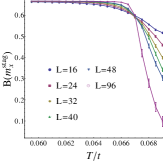
(a)

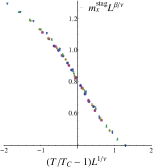
(b)

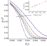
(c)

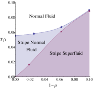
(d)

Figure 2: (a) Binder cumulants of the staggered magnetization $m^{\rm stag}_{x}$ for $L\times L$ systems at $\theta=\pi/2$, with $U\!=\!10t$, $\rho\!=\!0.94$, and $\Omega_{R}\!=\!0.5t$, showing crossing at $T_{\rm Ising}\!=\!0.067(1)t$. (b) Scaling collapse of the order parameter $m^{\rm stag}_{x}$ using Ising exponents $\beta\!=\!1/8$ and $\nu\!=\!1$. (c) Superfluid stiffness $\rho_{s}(T)$, showing finite size transition temperature $T_{c}(L)$ given by crossing of $\rho_{s}(T)$ with the line $2T/\pi$. Inset shows extrapolation of $T_{c}(L)$ to the thermodynamic limit, yielding $T_{\rm BKT}\!=\!0.0614(2)t$. (d) Doping-temperature phase diagram showing the emergence of a stripe normal phase.

Thermal fluctuations and transitions. — To study strong correlations at nonzero temperature $T=1/\beta$, we express the partition function $Z=\text{Tr}\left(e^{-\beta H}\right)$ in path integral form using the basis of Gutzwiller wavefunctions,

$$Z\!=\!\!\int\!{\cal D}\chi\chi^{*}\bra{\Psi}e^{-\beta H_{\rm eff}}\ket{\Psi}\!\!\approx\!\!\int\!{\cal D}\chi\chi^{*}e^{-\beta\bra{\Psi}H_{\rm eff}\ket{\Psi}},$$ (7)

where the final approximation uses the leading order term in a cumulant expansion. This cumulant approximation Stoudenmire et al. (2009) is exact at $T=0$, recovering the ground state energy with mean field quantum correlations, and is also exact to leading order in $1/T$ in a high temperature expansion (see Supplemental Material SuppMat for details). We thus expect this approximation to accurately capture thermal fluctuation effects over the entire range of temperatures.

To compute physical observables, we use a Monte Carlo approach to sample the partition function and calculate observables, treating $\chi_{i,n}$ as stochastically fluctuating variables. This method generalizes in a straightforward manner if we relax the no double-occupancy constraint to allow for a maximum occupancy $n_{\rm max}$ bosons at each site including both species. In this case, each site has a complex vector of $(n_{\rm max}+1)(n_{\rm max}+2)/2$ fluctuating components. Since there is no sign problem, this method is also suitable for studying thermal fluctuations in frustrated bosons and their Mott transitions.

For generic $\theta$, the Bose condensation wavevector and the magnetic order will be incommensurate, and will shift with $\Omega_{R}$ and $T$. This makes it numerically more difficult to accurately locate the thermal transitions. Here, we therefore illustrate this method by studying the effect of thermal fluctuations at $\theta=\pi/2$, which ensures that the ordering wavevector $Q=\pi/2$ is independent of $\Omega_{R}$ and $T$, enabling us to precisely locate the thermal transitions.

At $\theta=\pi/2$, the staggered magnetization, $m_{x}^{stag}\equiv\sum_{i}\left(-1\right)^{x_{i}}\langle S^{x}_{i}\rangle$, breaks $Z_{2}$ symmetry when $\Omega_{R}\neq 0$. To probe the transition where magnetism is lost, we compute the Binder cumulant Binder (1981) curves of the order parameter. As shown in Fig. 2(a), for $U/t=10$, $\rho=0.94$, $\Omega_{R}=0.5t$, these show a unique crossing point, which allows us to locate $T_{\rm Ising}=0.067(1)t$. We find, as shown in Fig. 2(b), that the scaled order parameter near $T_{\rm Ising}$ collapses onto a single curve for Ising exponents, $\beta=1/8$ and $\nu=1$.

We track the destruction of superfluid order by computing the superfluid stiffness. Since the Hamiltonian is anisotropic in space, the stiffness is different along $\hat{x}$ and $\hat{y}$, and the geometric mean $\rho_{s}\!=\!\sqrt{\rho_{s}^{xx}\rho_{s}^{yy}}$ controls the energy of vortices which proliferate and destroy superfluidity. As seen in Fig.2(c), $\rho_{s}$ drops rapidly with temperature reminiscent of the behavior near a Berezinskii-Kosterlitz-Thouless (BKT) transition. We confirm this by identifying the finite size superfluid transition temperature $T_{c}(L)$ via the intersection point defined by $\rho_{s}\left(T_{c}(L)\right)\!=\!2T_{c}(L)/\pi$, and finding that $T_{c}(L)$ obeys the expected scaling form $T_{C}(L)\!=\!T_{\rm BKT}\!+\!b/\ln^{2}(L/L_{0})$ (see Fig.2(c) inset), where $b$ and $L_{0}$ are non-universal numbers. This also allows us to extract the thermodynamic limit transition temperature $T_{\rm BKT}\!=\!0.0614(2)t$. We have confirmed the BKT nature of the transition from the critical scaling of $n(\bf{k})$ (see Supplemental Material SuppMat ).

Using the above methods to extract $T_{\rm Ising}$ and $T_{\rm BKT}$ at various densities $\rho$ enables us to construct the phase diagram in Fig. 2(d). In the Mott insulator, at $\rho=1$, we find a single (Ising) transition associated with magnetic ordering. Upon doping, the stripe magnetic order survives, but in addition superfluidity appears with a low transition temperature. This leads to a wide window of normal stripe order. With increasing doping away from the Mott insulator, the two transitions get closer to each other, and the normal stripe order shrinks.

Discussion. — For lattice bosons with SOC, we have uncovered strongly correlated superfluid ground states distinct from the continuum. At $T\!\neq\!0$, we have used a stochastic Gutzwiller approach to show that the $ST$ superfluid phase undergoes multiple transitions, revealing an intermediate stripe normal phase which increases in width as one approaches the Mott insulator. Going beyond our specific calculations, we expect that even for $\theta\!\neq\!\pi/2$, magnetic order will persist in the Mott insulator, whereas the superfluid transiton temperature $T_{\rm BKT}$ will vanish as $\rho\!\to\!1$; thus, the stripe normal phase will persist even in this generic case. Furthermore, even if the repulsion is not strong enough to drive Mott insulators, we expect the window of normal stripe fluid to be maximal near $\rho\sim 1$, and the stripe normal phase should also persist in higher dimensions. Our phase diagram could be explored using atomic bosons with SOC in optical lattices Hamner et al. (2014). The stripe normal fluid would display broadened momentum peaks simultaneously at $\pm Q$, visible in time-of-flight experiments. The spin order in the normal stripe fluid could be probed using Bragg scattering experiments Corcovilos et al. (2010), similar to recent detection of Néel correlations in the atomic Fermi-Hubbard model Hart et al. (2014).

Note added. — During completion of this manuscript we became aware of complementary work Radic2014 which discusses magnetic instabilities of normal (uncondensed) spin-1/2 bosons in the continuum.

Acknowledgements. — We thank I. Kivlichan, P. Engels, V. Galitski, S.-B. Lee, S. Natu, H. Pu, H. Zhai, and N. Trivedi for useful discussions. We acknowledge funding from NSERC of Canada. AP thanks the Aspen Center for Physics (Grant No. NSF PHY-1066293) for hospitality during the completion of this manuscript.

I. appendix

I..1 Derivation of $tJ$ model for two-component bosons with SOC

With the hyperfine flavours labelled by $c$ and $d$ the local Hubbard interaction is

$$H_{\rm U}=\frac{U_{cc}}{2}\sum_{i}n_{i,c}(n_{i,c}-1)+\frac{U_{dd}}{2}\sum_{i}n_{i,d}(n_{i,d}-1)+U_{cd}\sum_{i}n_{i,c}n_{i,d},$$ (8)

Setting $U=U_{cc}=U_{dd}$, $\lambda U=U_{cd}$ and $U\gg t$, we restrict ourselves to a Hilbert space in which double occupancy of sites is forbidden. Using second order perturbation theory in $t/U$ we can derive an effective Hamiltonian for this restricted space with $H_{\rm U}$ given by Eq. 8 and the perturbation $H_{\rm kin}$ given by Eq. 1. Written in terms of hyperfine basis states the perturbation $H_{\rm kin}$ is

$$H_{\rm kin}= -t\sum_{i}\left(e^{i\theta}c_{i}^{\dagger}c_{i+\hat{x}}+e^{-i\theta}d_{i}^{\dagger}d_{i+\hat{x}}+h.c.\right)-t\sum_{i}\left(c_{i}^{\dagger}c_{i+\hat{y}}+d_{i}^{\dagger}d_{i+\hat{y}}+h.c.\right)-\frac{\Omega_{R}}{2}\sum_{i}\left(c_{i}^{\dagger}d_{i}+d_{i}^{\dagger}c_{i}\right).$$ (9)

Using a two-site basis of degenerate states $\left[\ket{c,c},\ket{c,d},\ket{d,c},\ket{d,d}\right]$ the matrix form of the effective Hamiltonian for the $\hat{x}$-direction is

$$H^{J}_{x}=\begin{pmatrix}-\frac{4t^{2}}{U}&0&0&0\\ 0&-\frac{2t^{2}}{\lambda U}&-\frac{2t^{2}}{\lambda U}e^{2i\theta}&0\\ 0&-\frac{2t^{2}}{\lambda U}e^{-2i\theta}&-\frac{2t^{2}}{\lambda U}&0\\ 0&0&0&-\frac{4t^{2}}{U}\end{pmatrix},$$ (10)

while in the $\hat{y}$ direction

$$H^{J}_{y}=\begin{pmatrix}-\frac{4t^{2}}{U}&0&0&0\\ 0&-\frac{2t^{2}}{\lambda U}&-\frac{2t^{2}}{\lambda U}&0\\ 0&-\frac{2t^{2}}{\lambda U}&-\frac{2t^{2}}{\lambda U}&0\\ 0&0&0&-\frac{4t^{2}}{U}\end{pmatrix}.$$ (11)

These can be rewritten in terms of spin operators as:

$$H^{J}= \sum_{i}\sum_{\delta=\hat{x},\hat{y}}\left(\sum_{a=x,y,z}J_{\delta}^{a}S_{i}^{a}S_{i+\delta}^{a}\right)+\sum_{i}\mathbf{D}\cdot(\mathbf{S}_{i}\times\mathbf{S}_{i+\hat{x}}),$$ (12)

where $S_{i}^{x}=(b_{i\uparrow}^{\dagger}b_{i\downarrow}+b_{i\downarrow}^{\dagger}b_{i\uparrow})/2,\,S_{i}^{y}=-i(b_{i\uparrow}^{\dagger}b_{i\downarrow}-b_{i\downarrow}^{\dagger}b_{i\uparrow})/2$ and $S_{i}^{z}=(n_{i\uparrow}-n_{i\downarrow})/2$ and the exchange coefficients $J_{\delta}^{a}$ and Dzyaloshinskii-Moriya vectors are given in Table 1. The total Hamiltonian is then given by ${\cal P}H_{\rm kin}{\cal P}+H^{J}$, as given in Eq. 3 of the paper.

I..2 Details of finite temperature Gutzwiller method.

Using the basis of Gutzwiller wavefunctions the partition function can be written as

$$Z =\text{Tr}\left(e^{-\beta H}\right)=\int{\cal D}\chi\chi^{*}\bra{\Psi}e^{-\beta H}\ket{\Psi},$$

$$\approx\int{\cal D}\chi\chi^{*}e^{-\beta\bra{\Psi}H\ket{\Psi}},$$ (13)

where in the last line we have approximated it by the leading order term in a cumulant expansion of the full partition function and the integration measure is

$${\cal D}\chi\chi^{*}=\prod_{i}\left[\prod_{n}d\chi_{i,n}d\chi^{*}_{i,n}\right]\delta\left(\sum_{n}\left|\chi_{i,n}\right|^{2}-1\right).$$ (14)

where $0\leq n\leq n_{\rm max}$. Such a cumulant expansion has been used to study the appearance of quadrupolar correlations in a class of quantum spin-$1$ models in the literature Stoudenmire et al. (2009). At $T=0$ the approximation is exact, recovering the zero temperature Gutzwiller mean field result,

$$Z=\int{\cal D}\chi\chi^{*}e^{-\beta\bra{\Psi_{0}}H\ket{\Psi_{0}}}=\int{\cal D}\chi\chi^{*}e^{-\beta E_{0}}=\int{\cal D}\chi\chi^{*}\bra{\Psi_{0}}e^{-\beta H}\ket{\Psi_{0}}.$$

Furthermore, at high temperatures we can expand the exponential

$$Z \approx\int{\cal D}\chi\chi^{*}e^{-\beta\bra{\Psi}H\ket{\Psi}}\approx\int{\cal D}\chi\chi^{*}\left(1-\beta\bra{\Psi}H\ket{\Psi}+\ldots\right),$$

which matches exactly the high temperature expansion of the full partition function to leading order in $1/T$

$$Z =\int{\cal D}\chi\chi^{*}\bra{\Psi}e^{-\beta H}\ket{\Psi}\approx\int{\cal D}\chi\chi^{*}\bra{\Psi}\left(1-\beta H+\ldots\right)\ket{\Psi},$$

$$\approx\int{\cal D}\chi\chi^{*}\left(1-\beta\bra{\Psi}H\ket{\Psi}+\ldots\right).$$

We therefore expect this cumulant approximation to yield a good approximation to the full partition function and thermodynamic observables at all intermediate temperatures.

To sample the partition function, it is simplest to work in the grand canonical ensemble and make local updates on $\chi_{i,n}$ by choosing any two components at a randomly chosen site and performing a random $SU(2)$ rotation on them which explicitly preserves the normalization. We choose the chemical potential to leave the density fixed as we vary the temperature and magnetic field.

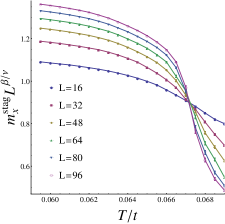
(a)

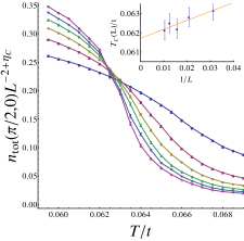
(b)

Figure 3: Plots of (a) the scaled staggered magnetization $m_{x}^{stag}L^{\beta/\nu}$ as a function of temperature $T$ for various system sizes $L\times L$, and (b) the scaled momentum distribution $n_{\rm tot}(\pi/2,0)L^{-2+\eta_{C}}$ (with $\eta_{C}=1/4$) for parameter values $U=10t,\lambda=0.95,\Omega_{R}=0.5t$ and a uniform density $\rho=0.94$.

I..3 Confirmation of the nature of the thermal transitions

Magnetic transition: We can obtain the magnetic transition temperature differently, by using the Ising nature of the magnetic critical point. We plot the scaled order parameter $m_{x}^{\rm stag}L^{\beta/\nu}$ with $\beta=1/8$ and $\nu=1$. There are three distinct behaviours expected for such a plot

$$\text{ Disordered ($T>T_{\rm Ising}$):}\,\,\,m_{x}^{\rm stag}L^{\beta/\nu} \sim L^{-1}L^{1/8}=L^{-7/8},$$

$$\text{Critical ($T=T_{\rm Ising}$):}\,\,\,m_{x}^{\rm stag}L^{\beta/\nu} \sim L^{0},$$

$$\text{Ordered ($T<T_{\rm Ising}$):}\,\,\,m_{x}^{\rm stag}L^{\beta/\nu} \sim L^{0}L^{1/8}=L^{1/8},$$ (15)

The curves are thus expected to cross at $T_{\rm Ising}$. The results are shown in Fig. 3(a) for $U=10t,\lambda=0.95,\Omega_{R}=0.5t$ and a uniform density $\rho=0.94$, yielding $T_{\rm Ising}=0.067(1)t$, in agreement with the Binder cumulant result.

Superfluid transition: To confirm the BKT nature of the superfluid transition we plot the scaled momentum distribution $n({{\bf{k}}})L^{-2+\eta_{C}}$ at ${{\bf{k}}}=\left(\pi/2,0\right)$ for different systems sizes $L$, where $\eta_{C}=1/4$ for a BKT transition. There are similarly three distinct behaviours expected

$$\text{ Disordered ($T>T_{\rm BKT}$):}\,\,\,n({{\bf{k}}})L^{-2+\eta_{C}} \sim L^{0}L^{-7/4}=L^{-7/4},$$

$$\text{Critical ($T=T_{\rm BKT}$):}\,\,\,n({{\bf{k}}})L^{-2+\eta_{C}} \sim L^{0},$$

$$\text{Algebraic Order ($T<T_{\rm BKT}$):}\,\,\,n({{\bf{k}}})L^{-2+\eta_{C}} \sim L^{2-\eta(T)}L^{-7/4}=L^{1/4-\eta(T)},$$ (16)

The numerical results are shown in Fig. 3(b) for $U=10t,\lambda=0.95,\Omega_{R}=0.5t$ and a uniform density $\rho=0.94$, with the crossing point clearly weakly drifting with system size $L$ due to logarithmic corrections to the superfluid stiffness at the BKT transition. In the inset, we plot the value of the crossing point for successive system sizes (called $T_{c}(L)$) as a function of $1/L$, where $L$ is the larger system size, which upon extrapolation to $L\to\infty$ yields $T_{\rm BKT}=0.0617(2)t$, in agreement with the result obtained from the superfluid stiffness calculation.

References

- Hasan and Kane (2010) M. Z. Hasan and C. L. Kane, Rev. Mod. Phys. 82, 3045 (2010).
- Qi and Zhang (2011) X.-L. Qi and S.-C. Zhang, Rev. Mod. Phys. 83, 1057 (2011).
- Haldane (1988) F. D. M. Haldane, Phys. Rev. Lett. 61, 2015 (1988).
- Chang et al. (2013) C.-Z. Chang, J. Zhang, X. Feng, J. Shen, Z. Zhang, M. Guo, K. Li, Y. Ou, P. Wei, L.-L. Wang, Z.-Q. Ji, Y. Feng, S. Ji, X. Chen, J. Jia, X. Dai, Z. Fang, S.-C. Zhang, K. He, Y. Wang, L. Lu, X.-C. Ma, and Q.-K. Xue, Science 340, 167 (2013).
- Yu et al. (2010) X. Z. Yu, Y. Onose, N. Kanazawa, J. H. Park, J. H. Han, Y. Matsui, N. Nagaosa, and Y. Tokura, Nature 465, 901 (2010).
- Pesin and Balents (2010) D. Pesin and L. Balents, Nat Phys 6, 376 (2010).
- Witczak-Krempa et al. (2014) W. Witczak-Krempa, G. Chen, Y. B. Kim, and L. Balents, Annual Review of Condensed Matter Physics 5, 57 (2014).
- Lin et al. (2011) Y.-J. Lin, K. Jimenez-Garcia, and I. B. Spielman, Nature 471, 83 (2011).
- Zhang et al. (2012) J.-Y. Zhang, S.-C. Ji, Z. Chen, L. Zhang, Z.-D. Du, B. Yan, G.-S. Pan, B. Zhao, Y.-J. Deng, H. Zhai, S. Chen, and J.-W. Pan, Phys. Rev. Lett. 109, 115301 (2012).
- Dalibard et al. (2011) J. Dalibard, F. Gerbier, G. Juzeliunas, and P. Ohberg, Rev. Mod. Phys. 83, 1523 (2011).
- LeBlanc et al. (2013) L. J. LeBlanc, M. C. Beeler, K. Jim nez-Garc a, A. R. Perry, S. Sugawa, R. A. Williams, and I. B. Spielman, New Journal of Physics 15, 073011 (2013).
- Qu et al. (2013) C. Qu, C. Hamner, M. Gong, C. Zhang, and P. Engels, Phys. Rev. A 88, 021604 (2013).
- Beeler et al. (2013) M. C. Beeler, R. A. Williams, K. Jimenez-Garcia, L. J. LeBlanc, A. R. Perry, and I. B. Spielman, Nature 498, 201 (2013), letter.
- Ji et al. (2014) S.-C. Ji, J.-Y. Zhang, L. Zhang, Z.-D. Du, W. Zheng, Y.-J. Deng, H. Zhai, S. Chen, and J.-W. Pan, Nat Phys 10, 314 (2014).
- Hamner et al. (2014) C. Hamner, Y. Zhang, M. A. Khamehchi, M. J. Davis, and P. Engels, ArXiv e-prints (2014), arXiv:1405.4048 [cond-mat.quant-gas] .
- Fu et al. (2014) Z. Fu, L. Huang, Z. Meng, P. Wang, L. Zhang, S. Zhang, H. Zhai, P. Zhang, and J. Zhang, Nat Phys 10, 110 (2014).
- Stanescu et al. (2008) T. D. Stanescu, B. Anderson, and V. Galitski, Phys. Rev. A 78, 023616 (2008).
- Wang et al. (2010) C. Wang, C. Gao, C.-M. Jian, and H. Zhai, Phys. Rev. Lett. 105, 160403 (2010).
- Ho and Zhang (2011) T.-L. Ho and S. Zhang, Phys. Rev. Lett. 107, 150403 (2011).
- Radić et al. (2011) J. Radić, T. A. Sedrakyan, I. B. Spielman, and V. Galitski, Phys. Rev. A 84, 063604 (2011).
- Li et al. (2012) Y. Li, L. P. Pitaevskii, and S. Stringari, Phys. Rev. Lett. 108, 225301 (2012).
- Martone et al. (2012) G. I. Martone, Y. Li, L. P. Pitaevskii, and S. Stringari, Phys. Rev. A 86, 063621 (2012).
- Chen and Zhai (2012) Z. Chen and H. Zhai, Phys. Rev. A 86, 041604 (2012).
- Li et al. (2013) Y. Li, G. I. Martone, L. P. Pitaevskii, and S. Stringari, Phys. Rev. Lett. 110, 235302 (2013).
- Lü and Sheehy (2013) Q.-Q. Lü and D. E. Sheehy, Phys. Rev. A 88, 043645 (2013).
- Jian and Zhai (2011) C.-M. Jian and H. Zhai, Phys. Rev. B 84, 060508 (2011).
- Ozawa and Baym (2012a) T. Ozawa and G. Baym, Phys. Rev. Lett. 109, 025301 (2012a).
- Barnett et al. (2012) R. Barnett, S. Powell, T. Graß, M. Lewenstein, and S. Das Sarma, Phys. Rev. A 85, 023615 (2012).
- Ozawa and Baym (2012b) T. Ozawa and G. Baym, Phys. Rev. A 85, 063623 (2012b).
- Anderson et al. (2013) B. M. Anderson, I. B. Spielman, and G. Juzeliunas, Phys. Rev. Lett. 111, 125301 (2013).
- Riedl et al. (2013) K. Riedl, C. Drukier, P. Zalom, and P. Kopietz, Phys. Rev. A 87, 063626 (2013).
- Sedrakyan et al. (2012) T. A. Sedrakyan, A. Kamenev, and L. I. Glazman, Phys. Rev. A 86, 063639 (2012).
- Ramachandhran et al. (2013) B. Ramachandhran, H. Hu, and H. Pu, Phys. Rev. A 87, 033627 (2013).
- Graß et al. (2011) T. Graß, K. Saha, K. Sengupta, and M. Lewenstein, Phys. Rev. A 84, 053632 (2011).
- Mandal et al. (2012) S. Mandal, K. Saha, and K. Sengupta, Phys. Rev. B 86, 155101 (2012).
- Cole et al. (2012) W. S. Cole, S. Zhang, A. Paramekanti, and N. Trivedi, Phys. Rev. Lett. 109, 085302 (2012).
- Radić et al. (2012) J. Radić, A. Di Ciolo, K. Sun, and V. Galitski, Phys. Rev. Lett. 109, 085303 (2012).
- Cai et al. (2012b) Z. Cai, X. Zhou, and C. Wu, Phys. Rev. A 85, 061605 (2012b).
- Xu et al. (2014) Z. Xu, W. S. Cole, and S. Zhang, Phys. Rev. A 89, 051604 (2014).
- Qian et al. (2013) Y. Qian, M. Gong, V. W. Scarola, and C. Zhang, ArXiv e-prints (2013), arXiv:1312.4011 [cond-mat.quant-gas] .
- Sun et al. (2014) F. Sun, J. Ye, and W.-M. Liu, ArXiv e-prints (2014), arXiv:1408.3399 [cond-mat.quant-gas] .
- He et al. (2014) L. He, A. Ji, and W. Hofstetter, ArXiv e-prints (2014), arXiv:1404.0970 [cond-mat.quant-gas] .
- Wong and Duine (2013) C. H. Wong and R. A. Duine, Phys. Rev. Lett. 110, 115301 (2013).
- (44) W. Han, S. Zhang, and W.-M. Liu, arXiv:1211.2097 (unpublished).
- (45) See Supplemental Material for details of (i) the strong coupling perturbation theory, (ii) the finite temperature Gutzwiller approach, and (iii) further numerical checks of the finite temperature phase transitions.
- Gutzwiller (1963) M. C. Gutzwiller, Phys. Rev. Lett. 10, 159 (1963).
- Krauth et al. (1992) W. Krauth, M. Caffarel, and J.-P. Bouchaud, Phys. Rev. B 45, 3137 (1992).
- Stoudenmire et al. (2009) E. M. Stoudenmire, S. Trebst, and L. Balents, Phys. Rev. B 79, 214436 (2009).
- Binder (1981) K. Binder, Zeitschrift f r Physik B Condensed Matter 43, 119 (1981).
- Corcovilos et al. (2010) T. A. Corcovilos, S. K. Baur, J. M. Hitchcock, E. J. Mueller, and R. G. Hulet, Phys. Rev. A 81, 013415 (2010).
- Hart et al. (2014) R. A. Hart, P. M. Duarte, T.-L. Yang, X. Liu, T. Paiva, E. Khatami, R. T. Scalettar, N. Trivedi, D. A. Huse, and R. G. Hulet, ArXiv e-prints (2014), arXiv:1407.5932 [cond-mat.quant-gas] .
- (52) J. Radic, S. Natu, and V. Galitski, Phys. Rev. Lett. 113 185302 (2014).