‘Riemann Equations’
in Bidifferential Calculus

Abstract

We consider equations that formally resemble a matrix Riemann (or Hopf) equation in the framework of bidifferential calculus. With different choices of a first-order bidifferential calculus, we obtain a variety of equations, including a semi-discrete and a fully discrete version of the matrix Riemann equation. A corresponding universal solution-generating method then either yields a (continuous or discrete) Cole-Hopf transformation, or leaves us with the problem of solving Riemann equations (hence an application of the hodograph method). If the bidifferential calculus extends to second order, solutions of a system of ‘Riemann equations’ are also solutions of an equation that arises, on the universal level of bidifferential calculus, as an integrability condition. Depending on the choice of bidifferential calculus, the latter can represent a number of prominent integrable equations, like self-dual Yang-Mills, as well as matrix versions of the two-dimensional Toda lattice, Hirota’s bilinear difference equation, (2+1)-dimensional NLS, KP and Davey-Stewartson equations. For all of them, a recent (non-isospectral) binary Darboux transformation result in bidifferential calculus applies, which can be specialized to generate solutions of the associated ‘Riemann equations’. For the latter, we clarify the relation between these specialized binary Darboux transformations and the aforementioned solution-generating method. From (arbitrary size) matrix versions of the ‘Riemann equations’ associated with an integrable equation, possessing a bidifferential calculus formulation, multi-soliton-type solutions of the latter can be generated. This includes ‘breaking’ multi-soliton-type solutions of the self-dual Yang-Mills and the (2+1)-dimensional NLS equation, which are parametrized by solutions of Riemann equations.

Keywords: bidifferential calculus, breaking soliton, Burgers equation, chiral model, Cole-Hopf transformation, Darboux transformation, Davey-Stewartson equation, Hirota bilinear difference equation, Hopf equation, hierarchy, integrable discretization, kink, KP, Riemann equation, self-dual Yang-Mills, soliton, Toda lattice.

1 Introduction

Given an associative algebra $\mathcal{A}$ and two derivations $\mathrm{d},\bar{\mathrm{d}}:\mathcal{A}\rightarrow\Omega^{1}$ into an $\mathcal{A}$-bimodule, the two equations

$$\bar{\mathrm{d}}\phi-(\mathrm{d}\phi)\,\phi=0$$ (1.1)

and

$$\bar{\mathrm{d}}\phi+\phi\,\mathrm{d}\phi=0\,,$$ (1.2)

for $\phi\in\mathcal{A}$, resemble a Riemann equation (also known as Hopf, inviscid Burgers, dispersionless KdV, or nonlinear transport equation). For a simple choice of the first-order bidifferential calculus, given by $\mathcal{A},\Omega^{1},\mathrm{d},\bar{\mathrm{d}}$, these are indeed matrix Riemann equations (see in particular [1, 2, 3, 4, 5, 6, 7, 8, 9, 10] for appearances in the literature). For other choices, (1.1) and (1.2) turn out to be very different equations, however. This is so because we allow $\phi$ to be an operator (e.g., a differential or difference operator), a familiar step in the theory of integrable systems, where one considers a ‘zero curvature’ (Zakharov-Shabat, or Lax) equation in general for operator expressions. Accordingly, $\mathcal{A}$ will then be an algebra involving operators. Several examples will be presented in this work. The most basic ones are semi and a full discretizations of matrix Riemann equations. The following table shows that they are obtained from the bidifferential calculus formulation for the continuous Riemann equation essentially by replacing operators $\partial_{x},\partial_{t}$ of taking the partial derivatives with respect to $x$, respectively $t$, by shift operators $\mathbb{S}_{0}$, respectively $\mathbb{S}_{1}$, acting on corresponding discrete variables.

$\mathrm{d}$	$\bar{\mathrm{d}}$		$\bar{\mathrm{d}}\phi-(\mathrm{d}\phi)\,\phi=0$
$[\partial_{x},\cdot]$	$[\partial_{t},\cdot]$	$\varphi=\phi$	$\varphi_{t}-\varphi_{x}\,\varphi=0$
$[\mathbb{S}_{0},\cdot]$	$[\partial_{t},\cdot]$	$\varphi=\phi\,\mathbb{S}_{0}$	$\varphi_{t}-(\varphi_{,0}-\varphi)\,\varphi=0$
$[\mathbb{S}_{1}^{-1}\mathbb{S}_{0},\cdot]$	$[\mathbb{S}_{1}^{-1},\cdot]$	$\varphi=\phi\,\mathbb{S}_{0}$	$\varphi_{,1}-\varphi-(\varphi_{,1}-\varphi_{,0})\,\varphi=0$

In these examples, $\mathcal{A}$ is the algebra of $m\times m$ matrices of functions, extended by shift operators in the last two cases. $\Omega^{1}$ is simply given by $\mathcal{A}$, $\varphi$ is a matrix of functions, and we set $\varphi_{,0}:=\mathbb{S}_{0}\varphi\mathbb{S}_{0}^{-1}$, $\varphi_{,1}:=\mathbb{S}_{1}\varphi\mathbb{S}_{1}^{-1}$. Since $\mathrm{d}$ and $\bar{\mathrm{d}}$ are given by commutators, they are obviously derivations. In all examples considered in this work, (1.1) and (1.2) are related by a transpose or adjoint operation. It is therefore sufficient to concentrate on (1.1).

Suppose there is an extension of the derivation $\mathrm{d}$ to a map $\mathcal{A}\stackrel{{\scriptstyle\mathrm{d}}}{{\rightarrow}}\Omega^{1}\stackrel{{\scriptstyle\mathrm{d}}}{{\rightarrow}}\Omega^{2}$, with another $\mathcal{A}$-bimodule $\Omega^{2}$, and correspondingly for $\bar{\mathrm{d}}$, such that

$$\mathrm{d}^{2}=\bar{\mathrm{d}}^{2}=\mathrm{d}\bar{\mathrm{d}}+\bar{\mathrm{d}}\mathrm{d}=0\,.$$ (1.3)

In this case we have a second-order bidifferential calculus, $(\Omega,\mathrm{d},\bar{\mathrm{d}})$, with $\Omega=\bigoplus_{r=0}^{2}\Omega^{r}$, $\Omega^{0}:=\mathcal{A}$ [11, 12]. Then, acting with $\mathrm{d}$ on (1.1) or (1.2) yields

$$\mathrm{d}\bar{\mathrm{d}}\phi+\mathrm{d}\phi\,\mathrm{d}\phi=0\,.$$ (1.4)

By choosing appropriate bidifferential calculi, this equation leads to various integrable partial differential and/or difference equations (PDDEs) (cf. [12] and references therein). A particular example is another semi-discretization of the Riemann equation, the (Lotka-) Volterra lattice equation (see Appendix Appendix A: Volterra lattice equation), which is not obtained from (1.1). Equations like (1.1), (1.2) and (1.4) are of a universal nature and integrable PDDEs, derived from them, can be thought of as realizations. Equation (1.4) originally arose from replacing $\mathrm{d}$ and $\bar{\mathrm{d}}$ by flat anticommuting ‘covariant derivatives’, as explained, e.g., in [12]. The use of a calculus similar to the calculus of differential forms on a manifold reduces otherwise lengthy and often rather intransparent computations to a few lines, simply by exploiting the Leibniz rule for $\mathrm{d}$ and $\bar{\mathrm{d}}$, and (1.3). Why are there two maps, $\mathrm{d}$ and $\bar{\mathrm{d}}$, instead of a single analog of the familiar exterior derivative? In this way the integrable structure underlying the self-dual Yang-Mills equation is expressed most concisely [12] and drastically generalized. Moreover, it generalizes the situation in Frölicher-Nijenhuis theory (cf. Remark 2.5 in [13]).

Some efficient solution generating methods can be easily derived for the universal equations. By choosing a bidifferential calculus in such a way that one of these equations becomes equivalent to some PDDE, the method applies to the latter, and in this way one typically obtains a method for that equation. In particular, this shows that solution generating methods for various equations have a surprisingly simple origin and a simple universal proof.

For some realizations of (1.1) (and (1.2)), there is a simple ‘linearization method’ (see Section 2), which in several cases is the origin of a Cole-Hopf-type transformation. Such realizations are in the class of ‘C-integrable equations’ (see, e.g., [14, 15, 16]). Matrix Burgers equations are the prototype examples. The method is ineffective for the Riemann equation, in which case the method of characteristics, or hodograph method, applies instead (cf. [8]).

A Cole-Hopf-type transformation does not extend to (1.4), for which, however, there is another universal method. Indeed, in [13] (also see Section 3), a solution-generating result representing an abstract version of binary Darboux transformations [17, 18] has been derived for (1.4) and the ‘(Miura-) dual’ equation

$$\mathrm{d}[(\bar{\mathrm{d}}g)\,g^{-1}]=0\,,$$ (1.5)

with (invertible) dependent variable $g\in\mathcal{A}$. More precisely, this is a solution generating result for the ‘Miura equation’

$$(\bar{\mathrm{d}}g)\,g^{-1}=\mathrm{d}\phi\,,$$ (1.6)

which has both equations, (1.4) and (1.5), as integrability conditions, provided that (1.3) holds. This binary Darboux transformation method requires solutions of versions of (1.1) and (1.2) as inputs (see (3.1)), which yields yet another motivation to explore these ‘Riemann equations’. In most cases, soliton families are obtained by choosing $\mathrm{d}$- and $\bar{\mathrm{d}}$-constant solutions of these equations, which are very special and somewhat trivial solutions. The non-autonomous chiral model equation that arises in integrable reductions of the vacuum Einstein (-Maxwell) equations is an important exception in this respect, see [19, 13] and also Section 5.1.3. More generally, this concerns equations possessing a non-isospectral linear problem (see [20, 21] and also, e.g., [22, 23]).

Furthermore, the present work partly originated from the simple observation that (1.6) becomes (1.1) (respectively (1.2)), if we set $g=\pm\phi$ (respectively $g^{-1}=\pm\phi$). The solution-generating result in [13] then still works and can indeed be applied to generate large classes of exact solutions of various realizations of (1.1) (respectively (1.2)). According to the implication

$$\bar{\mathrm{d}}\phi-(\mathrm{d}\phi)\,\phi=0\quad\Longrightarrow\quad\left\{\begin{array}[]{l}\mathrm{d}\bar{\mathrm{d}}\phi+(\mathrm{d}\phi)\,\mathrm{d}\phi=0\,,\\ \mathrm{d}[(\bar{\mathrm{d}}\phi)\,\phi^{-1}]=0\,,\end{array}\right.$$ (1.9)

assuming that the first order bidifferential calculus extends to second order, the system of equations given by a realization of (1.1) provides us with a special class of solutions of the associated realizations of (1.4) and (1.5). It is one of the main aims of this work to explore what this ‘Riemann system’ is for several integrable equations and what the corresponding class of solutions contains (see Sections 5-8). For example, the ‘Riemann system’ associated with the (matrix) KP equation consists of the first two members of a (matrix) Burgers hierarchy (see Section 7), so in this case the implication (1.9), with the upper equation on the right, expresses a well-known fact (cf. [24] and references cited there). The ‘Riemann system’ associated with the self-dual Yang-Mills equation consists of two matrix Riemann equations (see Section 5.1). Here we recover an observation made in [10]. In the case of the integrable non-autonomous chiral model underlying integrable reductions of the Einstein vacuum equations, the ‘Riemann system’ determines a matrix version of the pole trajectory equation of Belinski and Zakharov [25] (see Section 5.1.3). We also explore hitherto unknown ‘Riemann systems’ associated with several other integrable equations possessing a bidifferential calculus formulation.

In those cases where a ‘Riemann system’ admits a Cole-Hopf-type transformation, this is certainly the simplest way to generate exact solutions. Darboux transformations for PDDEs resulting from (1.1) (or (1.2)) are in this respect not the first choice, but may be helpful, depending on the addressed problem. We are particularly interested in understanding how the two methods are related. Of course, more general classes of solutions of (1.4) and (1.5) than those obtained from the associated ‘Riemann system’ can be generated using the binary Darboux transformation method (Theorem 3.1) and we will report more on this in a separate work.

Another aspect addressed in the present work concerns the way in which bidifferential calculi for many integrable equations are composed of those for ‘Riemann equations’.

The paper is organized as follows. Section 2 presents the aforementioned simple solution-generating method for (1.1). In Section 3 we recall from [13] the binary Darboux transformation theorem in bidifferential calculus, in a slightly generalized form, and specialize it in a corollary in the way described above. A simple, but crucial observation is that the theorem already works on the level of a first order bidifferential calculus and then applies to ‘Riemann equations’.

Section 4 treats matrix Riemann equations, their integrable (semi and full) discretizations, and corresponding hierarchies. In the semi-discrete case, this is the semi-discrete Burgers hierarchy first treated in [1]. The (fully) discrete Riemann hierarchy contains a matrix version of the discrete Burgers equation derived in [26]. We are not aware of previous explorations of its first member, an integrable discrete Riemann equation. Furthermore, the Darboux transformations derived for the matrix versions of the semi- and fully discrete Riemann equations are new to the best of our knowledge.

Sections 5-8 present a collection of important examples of (matrix versions of) integrable equations arising via (1.9) from a system of ‘Riemann equations’. This includes a generalization of Hirota’s bilinear difference equation, which we have not seen in the literature yet. In Section 6, we consider the (2+1)-dimensional Nonlinear Schrödinger (NLS) equation [27, 28, 29]. In particular, we show that ‘breaking solitons’ obtained in [30] are solutions of the associated ‘Riemann system’. Furthermore, we obtain matrix versions of these solutions and moreover multi-soliton solutions, which are parametrized by solutions of a ‘Riemann system’ (see Proposition 6.3). Section 7 presents the relation between the first two equations of a (matrix) Burgers hierarchy and the (matrix) KP equation as a special case of (1.9). Section 8 treats the Davey-Stewartson (DS) equation. In the scalar case, single dromion, soliton and solitoff solutions turn out to be solutions of the associated Riemann system. Section 9 contains some concluding remarks.

As above, also in the following Riemann equation, respectively Riemann system, without an adjective discrete or semi-discrete, will always refer to the familiar partial differential equation, respectively a system of such equations. In contrast, ‘Riemann equation’, respectively ‘Riemann system’, will refer to any equation, respectively a system of equations, that realizes (1.1) (which only in special cases becomes a Riemann equation or a Riemann system).

2 The linearization method

Writing

$$\phi=\Phi\,\phi_{0}\,\Phi^{-1}\,,$$ (2.1)

with an invertible $\Phi\in\mathcal{A}$, (1.1) is equivalent to

$$\bar{\mathrm{d}}\phi_{0}-(\mathrm{d}\phi_{0})\,\phi_{0}+[\gamma\,,\,\phi_{0}]=0\,,$$ (2.2)

where $\gamma\in\Omega^{1}$ is defined by

$$\bar{\mathrm{d}}\Phi-(\mathrm{d}\Phi)\,\phi_{0}-\Phi\,\gamma=0\,.$$ (2.3)

Let us, however, consider the last equation as an equation for $\Phi$, for a given $\gamma$. Then, if $\phi_{0}$ is a solution of (2.2), $\phi$ given by (2.1) solves (1.1). For fixed $\phi_{0}$, (2.1) and (2.3), written as linear equations for $\Phi$, can thus be regarded as a Lax pair for (1.1).

Here we only have to solve linear equations in order to construct new solutions. Obviously, (2.1) can only lead to a new solution if the solution $\Phi$ of the linear equation does not commute with $\phi_{0}$. This excludes the example of the scalar Riemann equation (see Section 4.1), but non-trivial solutions of matrix Riemann equations can be obtained (also see [8]). Since $\phi_{0}$ may involve an operator, (2.1) can also express a Cole-Hopf-type transformation. This includes the well-known Cole-Hopf transformation for the Burgers equation, see Section 7.

Remark 2.1.

(2.2) looks more general than (1.1). But if $\gamma$ does not depend on $\phi_{0}$, as assumed above, the $\gamma$ term in (2.2) can be absorbed via the redefinition $\bar{\mathrm{d}}\mapsto\bar{\mathrm{d}}-[\gamma,\cdot]$. Furthermore, replacing (2.3) by $\bar{\mathrm{d}}\Phi-(\mathrm{d}\Phi)\,\phi_{0}+[\gamma,\Phi]=0$, then $\phi$ given by (2.1) also satisfies (2.2).

Remark 2.2.

Instead of (1.1), we may consider the more general equation

$$\bar{\mathrm{d}}\phi-(\mathrm{d}\phi)\,\eta(\phi)=\rho(\phi)\,,$$ (2.4)

where the function $\eta$ and $\rho\in\Omega^{1}$ are required to satisfy $\eta(\phi)=\Phi\,\eta(\phi_{0})\,\Phi^{-1}$, $\rho(\phi)=\Phi\,\rho(\phi_{0})\,\Phi^{-1}$. (2.4) is then equivalent to

$$\bar{\mathrm{d}}\phi_{0}-(\mathrm{d}\phi_{0})\,\eta(\phi_{0})+[\gamma\,,\,\phi_{0}]=\rho(\phi_{0})\,,$$

where $\gamma\in\Omega^{1}$ is defined by

$$\bar{\mathrm{d}}\Phi-(\mathrm{d}\Phi)\,\eta(\phi_{0})-\Phi\,\gamma=0\,.$$

Considering these as equations for a given $\gamma$, everything works well as long as $\phi$ has values in an algebra of matrices of functions, which is then a case treated in [8]. If the algebra $\mathcal{A}$ contains operators and $\phi$ is an operator expression, it will typically be impossible to reduce (2.4) to a PDDE. There are exceptions when $\eta$ is homogeneous. However, in those cases we looked at, it turned out that they can also be treated starting from (1.1), see Remarks 4.14 and 4.15. In [8] also generalizations of matrix Riemann equations to any number of independent variables are treated. In principle, our formalism can incorporate this via a straight generalization of (2.4) and extending $\mathrm{d}$ to several commuting derivations $\mathrm{d}_{i}:\mathcal{A}\rightarrow\mathcal{A}$, $i=1,\ldots,N$. However, we have not been able to find a PDDE arising in this way outside of the (continuous) framework of [8].

3 Binary Darboux transformations in bidifferential calculus

In the following, let $\mathcal{A}$ be the algebra of all finite-dimensional matrices with entries in a unital associative algebra $\mathcal{B}$, where the product of two matrices is defined to be zero if the sizes of the two matrices do not match. We assume that there is an $\mathcal{A}$-bimodule $\Omega^{1}$ and derivations $\mathrm{d}$ and $\bar{\mathrm{d}}$ on $\mathcal{A}$ with values in $\Omega^{1}$, such that $\mathrm{d}$ and $\bar{\mathrm{d}}$ preserve the size of matrices. $\mathrm{Mat}(m,n,\mathcal{B})$ denotes the set of $m\times n$ matrices over $\mathcal{B}$. For fixed $m,n\in\mathbb{N}$, $I=I_{m}$ and $\boldsymbol{I}=I_{n}$ denote the $m\times m$, respectively $n\times n$, identity matrix, and we assume that they are constant with respect to $\mathrm{d}$ and $\bar{\mathrm{d}}$. Let us recall the main theorem in [13], in a slightly generalized form. It should be noticed, however, that here we do not require the conditions (1.3). All we need is that $\mathrm{d}$ and $\bar{\mathrm{d}}$ are derivations on $\mathcal{A}$, i.e., they satisfy the Leibniz rule.

Theorem 3.1.

Let $\phi_{0},g_{0}\in\mathrm{Mat}(m,m,\mathcal{B})$ solve (1.6), and let $\boldsymbol{P},\boldsymbol{Q}\in\mathrm{Mat}(n,n,\mathcal{B})$ be solutions of

$$\bar{\mathrm{d}}\boldsymbol{P}-(\mathrm{d}\boldsymbol{P})\,\boldsymbol{P}=-[\boldsymbol{\alpha}\,,\,\boldsymbol{P}]\,,\qquad\bar{\mathrm{d}}\boldsymbol{Q}-\boldsymbol{Q}\,\mathrm{d}\boldsymbol{Q}=[\boldsymbol{\beta}\,,\,\boldsymbol{Q}]\,,$$ (3.1)

with some $\boldsymbol{\alpha},\boldsymbol{\beta}\in\Omega^{1}$. Let $\boldsymbol{U}\in\mathrm{Mat}(m,n,\mathcal{B})$ and $\boldsymbol{V}\in\mathrm{Mat}(n,m,\mathcal{B})$ be solutions of the linear equations

$$\bar{\mathrm{d}}\boldsymbol{U}=(\mathrm{d}\boldsymbol{U})\,\boldsymbol{P}+(\mathrm{d}\phi_{0})\,\boldsymbol{U}+\boldsymbol{U}\,\boldsymbol{\alpha}\,,\qquad\bar{\mathrm{d}}\boldsymbol{V}=\boldsymbol{Q}\,\mathrm{d}\boldsymbol{V}-\boldsymbol{V}\,\mathrm{d}\phi_{0}+\boldsymbol{\beta}\,\boldsymbol{V}\,.$$ (3.2)

Furthermore, let $\boldsymbol{X}\in\mathrm{Mat}(n,n,\mathcal{B})$ be an invertible solution of the (inhomogeneous) linear equations

$$\boldsymbol{X}\,\boldsymbol{P}-\boldsymbol{Q}\,\boldsymbol{X}=\boldsymbol{V}\,\boldsymbol{U}\,,$$ (3.3)

$$\bar{\mathrm{d}}\boldsymbol{X}-(\mathrm{d}\boldsymbol{X})\,\boldsymbol{P}+(\mathrm{d}\boldsymbol{Q})\,\boldsymbol{X}+(\mathrm{d}\boldsymbol{V})\,\boldsymbol{U}=\boldsymbol{X}\,\boldsymbol{\alpha}+\boldsymbol{\beta}\,\boldsymbol{X}\,.$$ (3.4)

Then

$$\phi=\phi_{0}+\boldsymbol{U}\boldsymbol{X}^{-1}\boldsymbol{V}\qquad\mbox{and}\qquad g=(I+\boldsymbol{U}(\boldsymbol{Q}\,\boldsymbol{X})^{-1}\boldsymbol{V})\,g_{0}$$ (3.5)

yields a new solution of the Miura equation (1.6). $\square$

Remark 3.2.

For $\boldsymbol{\alpha}=\boldsymbol{\beta}=0$, the two equations in (3.1) are $n\times n$ matrix versions of (1.1) and (1.2), respectively. Unless $\boldsymbol{P}$ and $\boldsymbol{Q}$ are $\mathrm{d}$- and $\bar{\mathrm{d}}$-constant, the linear equations (3.2) constitute a non-isospectral problem (cf. [20, 21] and also, e.g., [22, 23]). $\boldsymbol{P}$ and $\boldsymbol{Q}$ may be regarded as operator (in particular, matrix) versions of a spectral parameter.

Remark 3.3.

Theorem 3.1 appeared in [13] with $\boldsymbol{\alpha}=\boldsymbol{\beta}=0$. Let us start with this version. Correspondingly, in this remark a reference to an equation in Theorem 3.1 shall mean the respective equation with $\boldsymbol{\alpha}=\boldsymbol{\beta}=0$. The introduction of $\boldsymbol{\alpha}$ and $\boldsymbol{\beta}$ is motivated by a freedom of transformations. Let us write

$$\boldsymbol{P}=\boldsymbol{\Psi}_{1}\tilde{\boldsymbol{P}}\boldsymbol{\Psi}_{1}^{-1}\,,\qquad\boldsymbol{Q}=\boldsymbol{\Psi}_{2}^{-1}\tilde{\boldsymbol{Q}}\boldsymbol{\Psi}_{2}\,,$$ (3.6)

with invertible $n\times n$ matrices $\boldsymbol{\Psi}_{1},\boldsymbol{\Psi}_{2}$. (3.1) then takes the form

$$\bar{\mathrm{d}}\tilde{\boldsymbol{P}}-(\mathrm{d}\tilde{\boldsymbol{P}})\,\tilde{\boldsymbol{P}}=-[\boldsymbol{\alpha}\,,\,\tilde{\boldsymbol{P}}]\,,\qquad\bar{\mathrm{d}}\tilde{\boldsymbol{Q}}-\tilde{\boldsymbol{Q}}\,\mathrm{d}\tilde{\boldsymbol{Q}}=[\boldsymbol{\beta}\,,\,\tilde{\boldsymbol{Q}}]\,,$$

where $\boldsymbol{\alpha},\boldsymbol{\beta}$ are now defined by

$$\bar{\mathrm{d}}\boldsymbol{\Psi}_{1}-(\mathrm{d}\boldsymbol{\Psi}_{1})\,\tilde{\boldsymbol{P}}=\boldsymbol{\Psi}_{1}\,\boldsymbol{\alpha}\,,\qquad\bar{\mathrm{d}}\boldsymbol{\Psi}_{2}-\tilde{\boldsymbol{Q}}\,\mathrm{d}\boldsymbol{\Psi}_{2}=\boldsymbol{\beta}\,\boldsymbol{\Psi}_{2}\,.$$

In terms of $\tilde{\boldsymbol{X}}:=\boldsymbol{\Psi}_{2}\boldsymbol{X}\boldsymbol{\Psi}_{1}$, $\tilde{\boldsymbol{U}}:=\boldsymbol{U}\boldsymbol{\Psi}_{1}$ and $\tilde{\boldsymbol{V}}:=\boldsymbol{\Psi}_{2}\boldsymbol{V}$, (3.3) and (3.4) are equivalent to

$$\tilde{\boldsymbol{X}}\,\tilde{\boldsymbol{P}}-\tilde{\boldsymbol{Q}}\,\tilde{\boldsymbol{X}}=\tilde{\boldsymbol{V}}\,\tilde{\boldsymbol{U}}\,,\qquad\bar{\mathrm{d}}\tilde{\boldsymbol{X}}-(\mathrm{d}\tilde{\boldsymbol{X}})\,\tilde{\boldsymbol{P}}+(\mathrm{d}\tilde{\boldsymbol{Q}})\,\tilde{\boldsymbol{X}}+(\mathrm{d}\tilde{\boldsymbol{V}})\,\tilde{\boldsymbol{U}}=\tilde{\boldsymbol{X}}\,\boldsymbol{\alpha}+\boldsymbol{\beta}\,\tilde{\boldsymbol{X}}\,,$$

where we used the linear equations for $\boldsymbol{\Psi}_{1}$ and $\boldsymbol{\Psi}_{2}$. The linear equations (3.2) are correspondingly transformed to

$$\bar{\mathrm{d}}\tilde{\boldsymbol{U}}=(\mathrm{d}\tilde{\boldsymbol{U}})\,\tilde{\boldsymbol{P}}+(\mathrm{d}\phi_{0})\,\tilde{\boldsymbol{U}}+\tilde{\boldsymbol{U}}\,\boldsymbol{\alpha}\,,\qquad\bar{\mathrm{d}}\tilde{\boldsymbol{V}}=\tilde{\boldsymbol{Q}}\,\mathrm{d}\tilde{\boldsymbol{V}}-\tilde{\boldsymbol{V}}\,\mathrm{d}\phi_{0}+\boldsymbol{\beta}\,\tilde{\boldsymbol{V}}\,.$$

The expressions (3.5) for the new solutions are invariant under $\boldsymbol{U}\mapsto\tilde{\boldsymbol{U}}$, $\boldsymbol{V}\mapsto\tilde{\boldsymbol{V}}$ and $\boldsymbol{X}\mapsto\tilde{\boldsymbol{X}}$. Abstracting $\boldsymbol{\alpha},\boldsymbol{\beta}$ from their above origin, leads to a slightly generalized version of Theorem 2.1 in [13], which is our Theorem 3.1. The freedom in the choice of $\boldsymbol{\alpha}$ and $\boldsymbol{\beta}$ turns out to be very helpful in order to derive a convenient expression for the solution of (3.3) and (3.4) in concrete examples.

Remark 3.4.

A particularly important observation is the following. If the ‘Riemann equations’ (3.1) are completely solvable via the method in Section 2, with (3.6) and $\mathrm{d}$- and $\bar{\mathrm{d}}$-constant $\tilde{\boldsymbol{P}}$ and $\tilde{\boldsymbol{Q}}$, then the computation in Remark 3.3 shows that Theorem 3.1 is equivalent to its restriction, where $\boldsymbol{P}$ and $\boldsymbol{Q}$ are $\mathrm{d}$- and $\bar{\mathrm{d}}$-constant and commute with $\boldsymbol{\alpha}$, respectively $\boldsymbol{\beta}$. In this case, (3.1) is redundant and Theorem 3.1 reduces to a method that generates solutions of (1.6) from solutions of only linear equations. We meet this situation if (1.1) is solvable by a Cole-Hopf transformation. But it does not hold if (1.1) (hence (3.1)) involves a Riemann equation.

The theorem includes a case, where solutions are generated from solutions of nonlinear ‘Riemann equations’, and the linear equations (3.2) are eliminated.

Corollary 3.5.

Let $\phi_{0},g_{0}\in\mathrm{Mat}(m,m,\mathcal{B})$ solve (1.6), and let $\boldsymbol{P},\boldsymbol{Q}\in\mathrm{Mat}(n,n,\mathcal{B})$ be solutions of

$$\bar{\mathrm{d}}\boldsymbol{P}-(\mathrm{d}\boldsymbol{P})\,\boldsymbol{P}=-[\boldsymbol{\alpha}\,,\,\boldsymbol{P}]\,,\qquad\bar{\mathrm{d}}\boldsymbol{Q}-\boldsymbol{Q}\,\mathrm{d}\boldsymbol{Q}=[\boldsymbol{\beta}\,,\,\boldsymbol{Q}]\,,$$

with $\boldsymbol{\alpha},\boldsymbol{\beta}\in\Omega^{1}$. Let $\boldsymbol{X}\in\mathrm{Mat}(n,n,\mathcal{B})$ be an invertible solution of the linear equations

$$\boldsymbol{X}\,\boldsymbol{P}-\boldsymbol{Q}\,\boldsymbol{X}=\boldsymbol{V}_{0}\,\boldsymbol{U}_{0}\,,\qquad\bar{\mathrm{d}}\boldsymbol{X}-(\mathrm{d}\boldsymbol{X})\,\boldsymbol{P}+(\mathrm{d}\boldsymbol{Q})\,\boldsymbol{X}=\boldsymbol{X}\,\boldsymbol{\alpha}+\boldsymbol{\beta}\,\boldsymbol{X}\,,$$

where $\boldsymbol{U}_{0}\in\mathrm{Mat}(m,n,\mathcal{B})$ and $\boldsymbol{V}_{0}\in\mathrm{Mat}(n,m,\mathcal{B})$ are $\mathrm{d}$- and $\bar{\mathrm{d}}$-constant. Then

$$\phi=\phi_{0}+\boldsymbol{U}_{0}\boldsymbol{X}^{-1}\boldsymbol{V}_{0}\qquad\mbox{and}\qquad g=(I+\boldsymbol{U}_{0}(\boldsymbol{Q}\,\boldsymbol{X})^{-1}\boldsymbol{V}_{0})\,g_{0}$$

yields a new solution of the Miura equation (1.6), if

$$(\mathrm{d}\phi_{0})\,\boldsymbol{U}_{0}+\boldsymbol{U}_{0}\,\boldsymbol{\alpha}=0\,,\qquad\boldsymbol{V}_{0}\,\mathrm{d}\phi_{0}-\boldsymbol{\beta}\,\boldsymbol{V}_{0}=0\,.$$ (3.7)

Proof.

This is obtained by choosing $\boldsymbol{U}$ and $\boldsymbol{V}$ to be $\mathrm{d}$- and $\bar{\mathrm{d}}$-constant in Theorem 3.1. (3.2) is then satisfied iff (3.7) holds. ∎

One way to satisfy (3.7) is to set $\boldsymbol{\beta}=-\boldsymbol{\alpha}=\boldsymbol{V}_{0}\,(\mathrm{d}\phi_{0})\,\boldsymbol{U}_{0}$, and $\boldsymbol{U}_{0}\boldsymbol{V}_{0}=I$ if $\mathrm{d}\phi_{0}\neq 0$.

The above results are of a very general algebraic nature and may also find applications in mathematical problems remote from differential or difference equations, which we address in this work. In the following sections we choose the graded algebra $\Omega$ to be of the form

$$\Omega=\mathcal{A}\otimes\bigwedge(\mathbb{C}^{K})\,,$$ (3.8)

where $\bigwedge(\mathbb{C}^{K})$ is the exterior (Grassmann) algebra of the vector space $\mathbb{C}^{K}$. In this case it is sufficient to define $\mathrm{d}$ and $\bar{\mathrm{d}}$ on $\mathcal{A}$. Then they extend to $\Omega$ by treating elements of $\bigwedge(\mathbb{C}^{K})$ as constants. We denote by $\xi_{1},\ldots,\xi_{K}$ a basis of $\bigwedge^{1}(\mathbb{C}^{K})$. Furthermore, we will henceforth assume that $\phi$ in (1.1) (or (1.2)) is an $m\times m$ matrix (with entries in a unital associative algebra $\mathcal{B}$).

3.1 Darboux transformations for ‘Riemann equations’

Now we state conditions under which Theorem 3.1 generates solutions of the special cases (1.1) and (1.2) of the Miura equation (1.6). These are the ‘Riemann equations’ on which we concentrate in this work.

Corollary 3.6.

Let $\phi_{0}$ be a solution of (1.1), respectively (1.2). Let $\boldsymbol{P},\boldsymbol{Q},\boldsymbol{U},\boldsymbol{V},\boldsymbol{X}$ be solutions of (3.1) - (3.4) and

$$\boldsymbol{Q}\,\boldsymbol{V}=\boldsymbol{V}\,\phi_{0}\,,\qquad\mbox{respectively}\qquad\boldsymbol{U}\,\boldsymbol{P}=-\phi_{0}\,\boldsymbol{U}\,.$$ (3.9)

Let $\phi$ be given by the expression in (3.5). Then $\phi$ is a solution of (1.1), respectively (1.2).

Proof.

Setting $g=\pm\phi$ in (1.6), turns it into (1.1). The additional condition, the first of (3.9), originates from evaluating $g=\pm\phi$ using the expressions (3.5) for $\phi$ and $g$. Correspondingly, setting $g^{-1}=\pm\phi$ in (1.6), it becomes (1.2). Using $g^{-1}=g_{0}^{-1}\,[I-\boldsymbol{U}\,(\boldsymbol{X}\boldsymbol{P})^{-1}\,\boldsymbol{V}]$, we are led to the second of (3.9). ∎

Remark 3.7.

As a consequence of the assumptions in Corollary 3.6, we obtain

$$(\boldsymbol{X}\boldsymbol{P}\boldsymbol{X}^{-1})\,\boldsymbol{V}=\boldsymbol{V}\phi\,,\qquad\mbox{respectively}\qquad\boldsymbol{U}\,(\boldsymbol{X}^{-1}\boldsymbol{Q}\boldsymbol{X})=-\phi\,\boldsymbol{U}\,.$$

These are counterparts of (3.9). If $n=m$ and $\boldsymbol{Q}=\phi_{0}=0$, so that the first of conditions (3.9) holds, and if $\boldsymbol{U}$ is invertible, then $\phi=\boldsymbol{U}\,\boldsymbol{P}\,\boldsymbol{U}^{-1}$. In this special case, the Corollary thus boils down to the method described in Section 2.

Remark 3.8.

Let $\mathcal{B}$ be an algebra of (real or complex) functions of independent variables. We assume the spectrum condition $\sigma(\boldsymbol{P})\cap\sigma(\boldsymbol{Q})=\emptyset$, and $n>m$. The first of (3.9) then implies that the $n\times nm$ matrix $(\boldsymbol{V}|\boldsymbol{Q}\boldsymbol{V}|\cdots|\boldsymbol{Q}^{n-1}\boldsymbol{V})=(\boldsymbol{V}|\boldsymbol{V}\phi_{0}|\cdots|\boldsymbol{V}\phi_{0}^{n-1})$ has at most $m$, hence less than $n$ linearly independent columns. In this case the pair $(\boldsymbol{Q},\boldsymbol{V})$ is said to be not controllable (see, e.g., [31]). A corresponding statement holds in case of the second of (3.9). Theorem 3 in [31] then says that (3.3) has no invertible solution, so that under the stated conditions the solution-generating method in Corollary 3.6 does not work. This concerns in particular the case of the Riemann equation (see Section 4.1). This negative result should not come as a surprise since ‘soliton methods’ are known not to work in case of hydrodynamic-type systems of which the Riemann equation is the prototype.

Remark 3.9.

In (2.2) we met an apparently generalized version of (1.1). By a redefinition of the derivation $\bar{\mathrm{d}}$, we can cast it into the form (1.1). In Theorem 3.1, we can perform the reverse step. The Miura equation then reads $(\bar{\mathrm{d}}g+[\gamma,g])\,g^{-1}=\mathrm{d}\phi$. Equations (3.1), (3.3), (3.4) and (3.5) remain unchanged, while (3.2) is modified to $\bar{\mathrm{d}}\boldsymbol{U}=(\mathrm{d}\boldsymbol{U})\,\boldsymbol{P}+(\mathrm{d}\phi_{0})\,\boldsymbol{U}+\boldsymbol{U}\,\boldsymbol{\alpha}-\gamma\,\boldsymbol{U}$ and $\bar{\mathrm{d}}\boldsymbol{V}=\boldsymbol{Q}\,\mathrm{d}\boldsymbol{V}-\boldsymbol{V}\,\mathrm{d}\phi_{0}+\boldsymbol{\beta}\,\boldsymbol{V}+\boldsymbol{V}\,\gamma$. The first part of Corollary 3.6 then holds correspondingly. For example, if the first of (3.9) is satisfied, and if $\phi_{0}$ solves (2.2), then $\phi$, given by the formula in (3.5), solves the same equation, i.e., $\bar{\mathrm{d}}\phi-(\mathrm{d}\phi)\,\phi+[\gamma\,,\,\phi]=0$.

4 Matrix Riemann equations and integrable discretizations

In this section, we consider the case $\Omega^{1}=\mathcal{A}$. $\mathrm{d}$ and $\bar{\mathrm{d}}$ then have to be derivations of $\mathcal{A}$.

4.1 Riemann equation

Let $\mathcal{A}$ be the algebra of matrices of (real or complex) smooth functions of independent variables $x,t$. For $f\in\mathcal{A}$, let

$$\mathrm{d}f=f_{x}\,,\qquad\bar{\mathrm{d}}f=f_{t}\,,$$

where a subscript indicates a partial derivative with respect to the corresponding independent variable. (1.1) is now the matrix Riemann equation

$$\phi_{t}=\phi_{x}\,\phi\,.$$ (4.1)

As a consequence of (4.1), the eigenvalues of $\phi$ satisfy the corresponding scalar version of this equation [2], hence a scalar Riemann equation. (2.1) only generates new solutions in the matrix case ($m>1$). Let $\phi_{0}$ be a solution of (4.1) that commutes with its partial derivatives. By use of the method of characteristics, solutions of (2.3), with $\gamma=0$, are then given by (also see [8])

$$\Phi=A_{0}+\sum_{i=1}^{k}A_{i}\,f_{i}(t\,\phi_{0}+x\,I)\,,$$

with any analytic functions $f_{i}$ and constant $m\times m$ matrices $A_{0},A_{i}$. (2.1) then yields a new solution of (4.1). According to Remark 3.8, our Corollary 3.6 is not helpful in this particular example.

4.2 Semi-discrete Riemann equation

Let $\mathcal{A}_{0}$ be the algebra of matrices of functions on $\mathbb{R}\times\mathbb{Z}$, smooth in the first variable $t$, and $\mathcal{A}=\mathcal{A}_{0}[\mathbb{S},\mathbb{S}^{-1}]$. For $f\in\mathcal{A}$, we set

$$\mathrm{d}f=[\mathbb{S},f]\,,\qquad\bar{\mathrm{d}}f=f_{t}\,,$$ (4.2)

where $\mathbb{S}$ is the shift operator in the discrete variable $k$. Then, in terms of

$$\varphi=\phi\,\mathbb{S}\,,$$ (4.3)

and using the notation

$$\varphi^{+}:=\mathbb{S}\varphi\mathbb{S}^{-1}\,,\qquad\varphi^{-}:=\mathbb{S}^{-1}\varphi\mathbb{S}\,,$$

(1.1) is the semi-discrete matrix Riemann equation

$$\varphi_{t}=(\varphi^{+}-\varphi)\,\varphi\,,$$ (4.4)

where $\varphi$ can now be restricted to be an $m\times m$ matrix of functions (not involving the shift operator explicitly). Such a matrix equation already appeared in [1]. The scalar version has been called ‘lattice Burgers equation’ in [32, 17, 33]. It also appears as a symmetry of a discrete Burgers equation in [26], and in a model for socio-economical systems in [34]. A lattice spacing $h$ can be introduced via a rescaling $t\mapsto t/h$. If $\varphi$, $\varphi_{t}$ and $(\varphi^{+}-\varphi)/h$ have limits as $h\to 0$, keeping $x:=k\,h$ fixed, then $\varphi$ solves the Riemann equation $\varphi_{t}=\varphi_{x}\,\varphi$.

Remark 4.1.

Let us fix $\varphi(k_{0},t)$ at some lattice point $k_{0}$. Writing (4.4) as $\varphi^{+}=\varphi+\varphi_{t}\,\varphi^{-1}$, as long as the inverse of $\varphi$ exists, extends this to a solution for $k>k_{0}$. To the left of $k_{0}$ on the lattice, we obtain from (4.4) iteratively at each lattice point (with $k<k_{0}$) a matrix Riccati equation:

$$\varphi_{t}(k_{0}-n,t)=-\varphi(k_{0}-n,t)^{2}+\varphi(k_{0}-n+1,t)\,\varphi(k_{0}-n,t)\qquad n=1,2,\ldots\,.$$

This presents another view of the integrability of (4.4) and, moreover, illustrates the ‘asymmetry’ arising from the presence of the forward difference in (4.4).

The alternative ‘Riemann equation’ (1.2) takes the form $\varphi_{t}=-\varphi\,(\varphi-\varphi^{-})$, which is obtained from (4.4) for the transpose of $\varphi$, if we replace $\mathbb{S}$ by its inverse. There is an alternative integrable semi-discretization of the Riemann equation, the (Lotka-) Volterra lattice equation, see Appendix Appendix A: Volterra lattice equation.

4.2.1 Cole-Hopf transformation

Choosing $\phi_{0}=\mathbb{S}^{-1}$, (2.1) becomes

$$\varphi=\Phi\,(\Phi^{-})^{-1}\,,$$ (4.5)

and (2.3) with $\gamma=A(t)$, where $A$ commutes with $\mathbb{S}$, takes the form

$$\Phi_{t}=\Phi^{+}-\Phi+\Phi\,A\,,$$ (4.6)

which for $A=0$ is a semi-discrete version of the transport equation. Since (4.4) is autonomous, if $\varphi$ is a solution, then also $\varphi^{+}$ is a solution. We can therefore redefine $\varphi$ and replace (4.5) by $\varphi=\Phi^{+}\,\Phi^{-1}$. Furthermore, we can eliminate $A$ by a redefinition of $\Phi$ that preserves (4.5). Equations (4.5) and (4.6) constitute a discrete Cole-Hopf transformation for the semi-discrete Riemann equation (4.4), also see [1, 32, 17].

Example 4.2.

A set of solutions of (4.6), with $A=0$, is given by

$$\Phi=I+\sum_{i=1}^{N}\boldsymbol{A}_{i}\,e^{\boldsymbol{\Theta}_{i}}\,\boldsymbol{B}_{i}\,,\qquad\boldsymbol{\Theta}_{i}:=\boldsymbol{\Lambda}_{i}\,k+(e^{\boldsymbol{\Lambda}_{i}}-\boldsymbol{I})\,t\,,$$

where $\boldsymbol{A}_{i}$ and $\boldsymbol{B}_{i}$ are constant $m\times n$, respectively $n\times m$ matrices, and the $\boldsymbol{\Lambda}_{i}$ are $n\times n$ matrices. In the scalar case ($m=1$), we can set $N=1$ without restriction of generality. Choosing $\boldsymbol{\Lambda}=\mathrm{diag}(\lambda_{1},\ldots,\lambda_{n})$, we obtain

$$\Phi=1+\sum_{i=1}^{n}e^{\theta_{i}}\,,\qquad\theta_{i}:=\lambda_{i}\,k+(e^{\lambda_{i}}-1)\,t+\gamma_{i}\,,$$ (4.7)

with constants $\gamma_{i}$. If the constants are real, then (4.5) yields an $n$-kink solution (see Fig. 1) of the scalar version of (4.4), cf. [32, 17]. In the continuum limit, such solutions become constant. Thus, regarding (4.4) as a discretization of the Riemann equation, the kink solutions are simply artifacts of the discretization. If $\boldsymbol{\Lambda}$ has non-diagonal Jordan normal form, further solutions are obtained. Examples of matrix shock wave solutions already appeared in [1], derived via Bäcklund transformations.

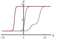
Figure 1: Plots (with interpolation) of a regular solution of the scalar semi-discrete Riemann equation (4.4), as given in Example 4.2, with $n=2$, $\lambda_{1}=1$, $\lambda_{2}=2$, $\gamma_{1}=\gamma_{2}=0$. Evolution in time $t$ is from right to left. For negative time, this is a $2$-kink solution (right curve), which turns into a single kink at $t=0$ (middle curve) and then becomes steeper and steeper (shock wave, left curve).

The scalar semi-discrete Riemann equation (4.4) is perhaps the simplest soliton equation (calling a kink a soliton). Although it is obtained via the simplest discretization from the Riemann equation, which is not a soliton equation (though integrable by the method of characteristics, or hodograph method), it is of a rather different nature. The behavior of the multiple kink solutions is actually very similar to that of corresponding solutions of the scalar Burgers equation, see Section 7. This is explained by the fact that (4.4) is a member of a semi-discrete Burgers hierarchy, see Remark 4.13 below.

Example 4.3.

We note that, if $\Phi$ has a nowhere vanishing continuum limit, then $\varphi$ tends to $I$. The kink solutions in Example 4.2 are corresponding examples. Setting $A=I$ in (4.6), and introducing the lattice spacing $h$, it reads $\Phi_{t}=\frac{1}{h}\Phi^{+}$, which is singular as $h\to 0$. In the scalar case ($m=1$), a particular solution is given by $\Phi=(-1)^{k+1}(k+1)!\,h^{k+2}t^{-(k+2)}$ for $h>0$. Although it has no limit as $h\to 0$, we find $\varphi=\Phi/\Phi^{-}=-(k+1)h/t\rightarrow-x/t$, which is a special solution of the Riemann equation.

Remark 4.4.

(4.5), written as $\Phi=\varphi\,\Phi^{-}$, together with (4.6) is a linear system that has (4.4) as its compatibility condition, hence the two equations constitute a Lax pair for (4.4). Choosing $A=(1-\lambda)\,I$, with a parameter $\lambda$, (4.6) reads

$$\Phi_{t}-\Phi^{+}+\lambda\,\Phi=0\,.$$

If $\Phi$ is a solution, then also $\Phi^{+}-\mu\,\Phi$, with any constant $\mu$. So we may replace (4.5) by $\Phi^{+}-\mu\,\Phi=\varphi\,(\Phi-\mu\,\Phi^{-})$ (now with a different $\varphi$), which is

$$\Phi^{+}=(\mu\,I+\varphi)\,\Phi-\mu\,\varphi\,\Phi^{-}\,.$$

Setting $\mu=2\,\lambda$, $\psi_{1}:=\Phi$ and $\psi_{2}:=\sqrt{2\lambda}\,\Phi^{-}$, we recover the Lax pair considered in [33] in the scalar case.

4.2.2 Darboux transformations

We exploit Corollary 3.6 in the case where $\boldsymbol{\alpha},\boldsymbol{\beta},\boldsymbol{P},\boldsymbol{Q}$ are constant. The restriction to $\mathrm{d}$- and $\bar{\mathrm{d}}$-constant $\boldsymbol{P}$ and $\boldsymbol{Q}$ is suggested by Remark 3.4. Setting

$$\boldsymbol{P}=\boldsymbol{A}\,\mathbb{S}^{-1}\,,\qquad\boldsymbol{Q}=\boldsymbol{B}\,\mathbb{S}^{-1}\,,\qquad\boldsymbol{X}=\mathbb{S}\,\tilde{\boldsymbol{X}}\,,$$

eliminates explicit appearances of the shift operator in the equations in Theorem 3.1. Then (3.1) is satisfied if $[\boldsymbol{\alpha},\boldsymbol{A}]=[\boldsymbol{\beta},\boldsymbol{B}]=0$. The remaining equations in Theorem 3.1 now take the form

$$\boldsymbol{U}_{t}=(\boldsymbol{U}^{+}-\boldsymbol{U})\,\boldsymbol{A}+(\varphi_{0}^{+}-\varphi_{0})\,\boldsymbol{U}+\boldsymbol{U}\,\boldsymbol{\alpha}\,,\qquad\boldsymbol{V}_{t}=\boldsymbol{B}\,(\boldsymbol{V}-\boldsymbol{V}^{-})-\boldsymbol{V}\,(\varphi_{0}^{+}-\varphi_{0})+\boldsymbol{\beta}\,\boldsymbol{V}\,,$$

and

$$\tilde{\boldsymbol{X}}^{+}\boldsymbol{A}-\boldsymbol{B}\,\tilde{\boldsymbol{X}}-\boldsymbol{V}\,\boldsymbol{U}=0\,,\qquad\tilde{\boldsymbol{X}}_{t}-(\tilde{\boldsymbol{X}}^{+}-\tilde{\boldsymbol{X}})\,\boldsymbol{A}+(\boldsymbol{V}-\boldsymbol{V}^{-})\,\boldsymbol{U}-\tilde{\boldsymbol{X}}\,\boldsymbol{\alpha}-\boldsymbol{\beta}\,\tilde{\boldsymbol{X}}=0\,,$$

which are compatible equations. By use of the first equation for $\tilde{\boldsymbol{X}}$, we can replace the second by

$$\tilde{\boldsymbol{X}}_{t}=\boldsymbol{V}^{-}\,\boldsymbol{U}+(\boldsymbol{\beta}+\boldsymbol{B})\,\tilde{\boldsymbol{X}}+\tilde{\boldsymbol{X}}\,(\boldsymbol{\alpha}-\boldsymbol{A})\,.$$

In the case under consideration, the first condition of (3.9) in Corollary 3.6 has to be considered, which here takes the form

$$\boldsymbol{B}\,\boldsymbol{V}^{-}=\boldsymbol{V}\,\varphi_{0}\,.$$

Using (4.3), the solution formula for $\phi$ in (3.5) reads

$$\varphi=\varphi_{0}+\boldsymbol{U}\tilde{\boldsymbol{X}}^{-1}\boldsymbol{V}^{-}\,.$$ (4.8)

In all these equations, we can now restrict $\varphi_{0},\boldsymbol{U},\boldsymbol{V},\tilde{\boldsymbol{X}}$ to $\mathcal{A}_{0}$, and $\boldsymbol{A}$, $\boldsymbol{B}$ to be matrices over $\mathbb{C}$.

Proposition 4.5.

Let $\varphi_{0}$ solve (4.4) and $\boldsymbol{U}$, $\boldsymbol{V}$ be solutions of

$$\boldsymbol{U}_{t}=\boldsymbol{U}^{+}\boldsymbol{A}+(\varphi_{0}^{+}-\varphi_{0})\,\boldsymbol{U}\,,\qquad\boldsymbol{V}_{t}=-\boldsymbol{V}\varphi_{0}^{+}\,,\qquad\boldsymbol{B}\boldsymbol{V}^{-}=\boldsymbol{V}\varphi_{0}\,,$$ (4.9)

with constant $n\times n$ matrices $\boldsymbol{A}$, $\boldsymbol{B}$. Then a new solution of (4.4) is given by (4.8) with

$$\tilde{\boldsymbol{X}}=\boldsymbol{C}^{-}+\int_{0}^{t}\boldsymbol{V}^{-}\boldsymbol{U}\,dt\,,$$ (4.10)

where $\boldsymbol{C}$ does not depend on $t$ and satisfies the constraint

$$\boldsymbol{C}\boldsymbol{A}-\boldsymbol{B}\boldsymbol{C}^{-}=\boldsymbol{V}\boldsymbol{U}\Big{|}_{t=0}\,.$$ (4.11)

Proof.

We choose $\boldsymbol{\alpha}=\boldsymbol{A}$ and $\boldsymbol{\beta}=-\boldsymbol{B}$. Then $\tilde{\boldsymbol{X}}_{t}=\boldsymbol{V}^{-}\,\boldsymbol{U}$, which integrates to the stated expression. It remains to solve $\tilde{\boldsymbol{X}}^{+}\boldsymbol{A}-\boldsymbol{B}\,\tilde{\boldsymbol{X}}=\boldsymbol{V}\,\boldsymbol{U}$. It is sufficient to do this at $t=0$, where $\tilde{\boldsymbol{X}}=\boldsymbol{C}^{-}$, and this leads to (4.11). ∎

Remark 4.6.

In the scalar case ($m=1$), under the conditions specified in Proposition 4.5, we have

$$\varphi=\varphi_{0}+\mathrm{tr}(\boldsymbol{V}^{-}\,\boldsymbol{U}\tilde{\boldsymbol{X}}^{-1})=\varphi_{0}+\mathrm{tr}(\tilde{\boldsymbol{X}}_{t}\tilde{\boldsymbol{X}}^{-1})=\varphi_{0}+(\ln\det\tilde{\boldsymbol{X}})_{t}\,.$$

Alternatively, we can write

$$\varphi = \varphi_{0}+\mathrm{tr}(\boldsymbol{V}^{-}\,\boldsymbol{U}\tilde{\boldsymbol{X}}^{-1})=\varphi_{0}\,(1+\mathrm{tr}(\boldsymbol{B}^{-1}\boldsymbol{V}\,\boldsymbol{U}\,\tilde{\boldsymbol{X}}^{-1}))=\varphi_{0}\,(1+\boldsymbol{U}\,\tilde{\boldsymbol{X}}^{-1}\,\boldsymbol{B}^{-1}\boldsymbol{V})$$

$$= \varphi_{0}\,\det(\boldsymbol{I}+\boldsymbol{B}^{-1}\boldsymbol{V}\,\boldsymbol{U}\,\tilde{\boldsymbol{X}}^{-1})=\varphi_{0}\,\det\Big{(}\boldsymbol{I}+\boldsymbol{B}^{-1}\,(\tilde{\boldsymbol{X}}^{+}\boldsymbol{A}-\boldsymbol{B}\,\tilde{\boldsymbol{X}})\,\tilde{\boldsymbol{X}}^{-1}\Big{)}$$

$$= \varphi_{0}\,\det(\tilde{\boldsymbol{X}}^{+}\,\boldsymbol{A}\,\tilde{\boldsymbol{X}}^{-1}\,\boldsymbol{B}^{-1})=\varphi_{0}\,\det(\boldsymbol{A})\,\det(\boldsymbol{B})^{-1}\,\det(\tilde{\boldsymbol{X}})^{+}\,\det(\tilde{\boldsymbol{X}})^{-1}\,,$$

using Sylvester’s determinant theorem in the fourth step. This makes contact with the Cole-Hopf transformation (4.5).

Example 4.7.

We consider the scalar case and set $\varphi_{0}=\mu\in\mathbb{C}\setminus\{0\}$, $\boldsymbol{A}=\boldsymbol{B}=\mu\,\boldsymbol{I}$. Writing $\boldsymbol{U}=(u_{1},\ldots,u_{n})$ and $\boldsymbol{V}=(v_{1},\ldots,v_{n})^{\intercal}$ (where ^⊺ denotes the transpose), the equations in (4.9) are solved by

$$u_{j}=(e^{\lambda_{j}}-1)\,e^{\lambda_{j}\,k+\mu\,e^{\lambda_{j}}\,t+\gamma_{j}}\,,\qquad v_{j}=\mu\,e^{-\mu\,t}\,,\qquad\lambda_{j},\gamma_{j}\in\mathbb{C}\,,\qquad j=1,\ldots,n\,.$$

(4.10) and (4.11) are then solved by

$$\tilde{\boldsymbol{X}}=\left(c_{ij}+e^{\theta_{j}}\right)_{i,j=1}^{n}\,,$$

where $c_{ij}$ are arbitrary constants, which we choose as $\delta_{ij}$, and $\theta_{i}:=\lambda_{i}\,k+\mu\,(e^{\lambda_{i}}-1)\,t+\gamma_{i}$. Using Sylvester’s determinant theorem, we obtain $\det\tilde{\boldsymbol{X}}=1+\sum_{j=1}^{n}e^{\theta_{j}}$, which is (4.7) if we set $\mu=1$. The latter can be achieved by an obvious scaling symmetry of (4.4).

4.3 Discrete Riemann equation

Let $\mathcal{A}_{0}$ be the algebra of matrices of functions on $\mathbb{Z}^{2}$. Let $\mathbb{S}_{0},\mathbb{S}_{1}$ be the corresponding commuting shift operators and $\mathcal{A}=\mathcal{A}_{0}[\mathbb{S}_{0}^{\pm 1},\mathbb{S}_{1}^{\pm 1}]$. We will use the notation

$$f_{,0}:=\mathbb{S}_{0}\,f\,\mathbb{S}_{0}^{-1}\,,\qquad f_{,1}:=\mathbb{S}_{1}\,f\,\mathbb{S}_{1}^{-1}\,,$$

and also $f_{,-0}:=\mathbb{S}_{0}^{-1}\,f\,\mathbb{S}_{0}$, $f_{,-1}:=\mathbb{S}_{1}^{-1}\,f\,\mathbb{S}_{1}$. Let

$$\mathrm{d}f=\frac{1}{h_{0}}\,[\mathbb{S}_{1}^{-1}\mathbb{S}_{0},f]\,,\qquad\bar{\mathrm{d}}f=\frac{1}{h_{1}}\,[\mathbb{S}_{1}^{-1},f]\,,$$

with constants $h_{0},h_{1}\neq 0$. In terms of

$$\varphi=\phi\,\mathbb{S}_{0}\,,$$

Equation (1.1) becomes

$$\frac{1}{h_{1}}\,(\varphi_{,1}-\varphi) = \frac{1}{h_{0}}\,(\varphi_{,1}-\varphi_{,0})\,\varphi$$ (4.12)

$$= \frac{1}{h_{0}}\,(\varphi_{,1}-\varphi)\,\varphi-\frac{1}{h_{0}}\,(\varphi_{,0}-\varphi)\,\varphi\,.$$

If $h_{0}=-1$, this formally tends to the semi-discrete Riemann equation (4.4) as $h_{1}\to 0$. In the following we set $h_{0}=h_{1}=1$, hence we consider the discrete matrix Riemann equation

$$\varphi_{,1}-\varphi=(\varphi_{,1}-\varphi_{,0})\,\varphi\,,$$ (4.13)

which can be rewritten as $\varphi_{,1}=(I-\varphi_{,0})\,\varphi\,(I-\varphi)^{-1}$.

(1.2) has the form $\varphi_{,0,1}-\varphi_{,0}=-\varphi_{,0,1}\,(\varphi_{,0}-\varphi_{,1})$, which becomes (4.13) for the transpose of $\varphi$, if we replace the two shift operators by their inverses.

4.3.1 Cole-Hopf transformation

Choosing $\phi_{0}=\mathbb{S}_{0}^{-1}$ in (2.1) and $\gamma=-A\,\mathbb{S}_{1}^{-1}$ in (2.3), with $A_{,0}=A$, we obtain for (4.13) the discrete Cole-Hopf transformation

$$\varphi=\Phi\,\Phi_{,-0}^{-1}\,,\qquad\Phi_{,0}-\Phi=(\Phi A)_{,1}\,.$$ (4.14)

Example 4.8.

A set of solutions of the linear equation in (4.14), with the choice $A=-I$, is given by

$$\Phi=\sum_{i=1}^{N}\boldsymbol{A}_{i}\,\boldsymbol{\Lambda}_{i}^{k_{0}}\,(I-\boldsymbol{\Lambda}_{i})^{k_{1}}\,\boldsymbol{B}_{i}\,,$$

where $\boldsymbol{A}_{i}$ and $\boldsymbol{B}_{i}$ are constant $m\times n$, respectively $n\times m$ matrices, and the $\boldsymbol{\Lambda}_{i}$ are constant $n\times n$ matrices. In the scalar case ($m=1$), we can set $N=1$ without restriction of generality. Choosing $\boldsymbol{\Lambda}=\mathrm{diag}(\lambda_{1},\ldots,\lambda_{n})$, we obtain

$$\Phi=\sum_{i=1}^{n+1}\gamma_{i}\,\lambda_{i}^{k_{0}}\,(1-\lambda_{i})^{k_{1}}\,,$$

with constants $\gamma_{i}$. If the constants are real and $\gamma_{i}>0$, $0<\lambda_{i}<1$, then (4.14) yields an $n$-kink solution of the scalar version of (4.13), also see Fig. 2. We can write the last expression in the form

$$\Phi=\mu^{k_{0}}\,(1-\mu)^{k_{1}}\,\Big{(}1+\sum_{i=1}^{n}\gamma_{i}\,\lambda_{i}^{k_{0}}\,\Big{(}\frac{1-\mu\lambda_{i}}{1-\mu}\Big{)}^{k_{1}}\Big{)}\,,$$ (4.15)

after the redefinitions $\lambda_{1}\mapsto\mu$, $\lambda_{i+1}/\lambda_{1}\mapsto\lambda_{i}$, $\gamma_{i+1}/\gamma_{1}\mapsto\gamma_{i}$, $i=1,\ldots,n$, and a rescaling of $\Phi$ that preserves $\varphi$.

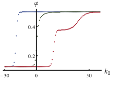
Figure 2: A regular $2$-kink solution of the scalar discrete Riemann equation (4.13) obtained via the discrete Cole-Hopf transformation (4.14) with (4.15), where we chose $\mu=1/2$, $\lambda_{1}=1/4$, $\lambda_{2}=3/4$, $\gamma_{1}=\gamma_{2}=1$. The plots, from left to right, correspond to consecutive values ($-50,0,50$) of $k_{1}$.

Remark 4.9.

Choosing $A=-\lambda\,I$, with a constant $\lambda$, the second equation in (4.14) reads

$$\Phi_{,0}-\Phi+\lambda\,\Phi_{,1}=0\,.$$

Writing the first equation in (4.14) as a linear equation for $\Phi$, we have a Lax pair for the discrete Riemann equation, with spectral parameter $\lambda$. If $\Phi$ is a solution of the above equation, then also $\Phi_{,0}-\mu\,\Phi$, with any constant $\mu$. We may thus replace the first equation in (4.14) by

$$\Phi_{,0}=(\mu\,I+\varphi)\,\Phi-\mu\,\varphi\,\Phi_{,-0}$$

(with a different $\varphi$). This is the counterpart of the corresponding Lax pair for the semi-discrete Riemann equation, see Remark 4.4.

4.3.2 Darboux transformations

In Corollary 3.6 we are led to set

$$\boldsymbol{\alpha}=\tilde{\boldsymbol{\alpha}}\mathbb{S}_{1}^{-1}\,,\quad\boldsymbol{\beta}=\tilde{\boldsymbol{\beta}}\,\mathbb{S}_{1}^{-1}\,,\quad\boldsymbol{P}=\boldsymbol{A}\,\mathbb{S}_{0}^{-1}\,,\quad\boldsymbol{Q}=\boldsymbol{B}\,\mathbb{S}_{0}^{-1}\,,\quad\boldsymbol{X}=\tilde{\boldsymbol{X}}\mathbb{S}_{0}\,,$$

with constant matrices $\tilde{\boldsymbol{\alpha}},\tilde{\boldsymbol{\beta}},\boldsymbol{A},\boldsymbol{B}$. Then (3.1) is satisfied if $[\tilde{\boldsymbol{\alpha}},\boldsymbol{A}]=[\tilde{\boldsymbol{\beta}},\boldsymbol{B}]=0$. The remaining equations we have to consider now take the form

$$\boldsymbol{U}-\boldsymbol{U}_{,1}=(\boldsymbol{U}_{,0}-\boldsymbol{U}_{,1})\,\boldsymbol{A}+(\varphi_{0,0}-\varphi_{0,1})\,\boldsymbol{U}+\boldsymbol{U}_{,1}\,\tilde{\boldsymbol{\alpha}}\,,$$

$$\boldsymbol{V}_{,1}-\boldsymbol{V}=\boldsymbol{B}\,(\boldsymbol{V}_{,-0,1}-\boldsymbol{V})-\boldsymbol{V}_{,1}\,(\varphi_{0,1}-\varphi_{0,0})-\tilde{\boldsymbol{\beta}}\,\boldsymbol{V}\,,$$

and

$$\tilde{\boldsymbol{X}}_{,0}\boldsymbol{A}-\boldsymbol{B}\,\tilde{\boldsymbol{X}}-\boldsymbol{V}_{,0}\,\boldsymbol{U}_{,0}=0\,,$$

$$\tilde{\boldsymbol{X}}_{,1}-\tilde{\boldsymbol{X}}-(\tilde{\boldsymbol{X}}_{,1}-\tilde{\boldsymbol{X}}_{,0})\boldsymbol{A}+(\boldsymbol{V}_{,1}-\boldsymbol{V}_{,0})\,\boldsymbol{U}_{,0}+\tilde{\boldsymbol{X}}_{,1}\,\tilde{\boldsymbol{\alpha}}+\tilde{\boldsymbol{\beta}}\,\tilde{\boldsymbol{X}}=0\,.$$

By use of the first equation for $\tilde{\boldsymbol{X}}$, we can replace the second by

$$\tilde{\boldsymbol{X}}_{,1}-\tilde{\boldsymbol{X}}+\tilde{\boldsymbol{X}}_{,1}\,(\tilde{\boldsymbol{\alpha}}-\boldsymbol{A})+(\tilde{\boldsymbol{\beta}}+\boldsymbol{B})\,\tilde{\boldsymbol{X}}+\boldsymbol{V}_{,1}\,\boldsymbol{U}_{,0}=0\,.$$

We have to consider the first condition of (3.9), which here takes the form

$$\boldsymbol{B}\,\boldsymbol{V}=\boldsymbol{V}_{,0}\,\varphi_{0,0}\,.$$

The solution formula in (3.5) reads

$$\varphi=\varphi_{0}+\boldsymbol{U}(\tilde{\boldsymbol{X}}^{-1}\boldsymbol{V})_{,-0}\,.$$ (4.16)

We can now restrict $\varphi_{0},\boldsymbol{U},\boldsymbol{V},\tilde{\boldsymbol{X}}$ to $\mathcal{A}_{0}$.

Proposition 4.10.

Let $\varphi_{0}$ solve (4.13), and let $\boldsymbol{U}$, $\boldsymbol{V}$ be solutions of the linear equations

$$\boldsymbol{U}_{,1}-\boldsymbol{U}+\boldsymbol{U}_{,0}\,\boldsymbol{A}=(\varphi_{0,1}-\varphi_{0})\,\boldsymbol{U}\,,$$

$$\boldsymbol{B}\,\boldsymbol{V}_{,-0}=\boldsymbol{V}\,\varphi_{0}\,,\qquad\boldsymbol{V}_{,1}-\boldsymbol{V}=\boldsymbol{V}_{,1}\,\varphi_{0,0}\,,$$

with constant matrices $\boldsymbol{A}$, $\boldsymbol{B}$. Let

$$\tilde{\boldsymbol{X}}(k_{0},k_{1})=\boldsymbol{F}(k_{0})-\left\{\begin{array}[]{l}\sum_{j=0}^{k_{1}-1}\boldsymbol{V}(k_{0},j+1)\,\boldsymbol{U}(k_{0}+1,j)\\ \sum_{j=k_{1}-1}^{0}\boldsymbol{V}(k_{0},j+1)\,\boldsymbol{U}(k_{0}+1,j)\end{array}\right.\quad\mbox{if}\quad\begin{array}[]{l}k_{1}\geq 1\\ k_{1}<1\end{array}\,,$$

where $k_{0}$ and $k_{1}$ are the discrete variables on which the shift operators $\mathbb{S}_{0}$, respectively $\mathbb{S}_{1}$ act, and $\boldsymbol{F}$ is an arbitrary $n\times n$ matrix function satisfying

$$\boldsymbol{F}(k_{0}+1)\,\boldsymbol{A}-\boldsymbol{B}\boldsymbol{F}(k_{0})-\boldsymbol{V}(k_{0}+1,0)\,\boldsymbol{U}(k_{0}+1,0)=0\,.$$

Then a new solution of (4.13) is given by (4.16).

Proof.

We choose $\tilde{\boldsymbol{\alpha}}=\boldsymbol{A}$ and $\tilde{\boldsymbol{\beta}}=-\boldsymbol{B}$. Then the equations for $\tilde{\boldsymbol{X}}$ read

$$\tilde{\boldsymbol{X}}_{,1}-\tilde{\boldsymbol{X}}+\boldsymbol{V}_{,1}\,\boldsymbol{U}_{,0}=0\,,\qquad\tilde{\boldsymbol{X}}_{,0}\,\boldsymbol{A}-\boldsymbol{B}\,\tilde{\boldsymbol{X}}=\boldsymbol{V}_{,0}\,\boldsymbol{U}_{,0}\,.$$

The first equation is completely solved by the expression for $\tilde{\boldsymbol{X}}$ in the proposition. The second equation then results in the stated constraint. ∎

Remark 4.11.

In the scalar case, we have

$$\varphi = \varphi_{0}\,(1+\boldsymbol{U}\tilde{\boldsymbol{X}}_{,-0}^{-1}\boldsymbol{B}^{-1}\boldsymbol{V})=\varphi_{0}\,\det(\boldsymbol{I}+\boldsymbol{B}^{-1}\boldsymbol{V}\,\boldsymbol{U}\tilde{\boldsymbol{X}}_{,-0}^{-1})$$ (4.18)

$$= \varphi_{0}\,\det\Big{(}\boldsymbol{I}+\boldsymbol{B}^{-1}\,(\tilde{\boldsymbol{X}}\,\boldsymbol{A}-\boldsymbol{B}\,\tilde{\boldsymbol{X}}_{,-0})\,\tilde{\boldsymbol{X}}_{,-0}^{-1}\Big{)}$$

$$= \varphi_{0}\,\det(\boldsymbol{A})\,\det(\boldsymbol{B})^{-1}\,\det(\tilde{\boldsymbol{X}})\,\det(\tilde{\boldsymbol{X}})_{,-0}^{-1}\,,$$

which makes contact with the Cole-Hopf transformation.

Example 4.12.

Let $m=1$ (scalar case) and $\varphi_{0}=\mu\in\mathbb{C}\setminus\{0,1\}$, $\boldsymbol{A}=\boldsymbol{B}=\mu\,\boldsymbol{I}$. Writing $\boldsymbol{U}=(u_{1},\ldots,u_{n})$ and $\boldsymbol{V}=(v_{1},\ldots,v_{n})^{\intercal}$, the linear equations for $\boldsymbol{U}$ and $\boldsymbol{V}$ are solved by

$$u_{j}=a_{j}\lambda_{j}^{k_{0}-1}(1-\lambda_{j}\mu)^{k_{1}}\,,\qquad v_{j}=(1-\mu)^{-k_{1}}\,,\qquad a_{j},\lambda_{j}\in\mathbb{C}\,,\qquad j=1,\ldots,n\,.$$

$\tilde{\boldsymbol{X}}$ is then given by

$$\tilde{\boldsymbol{X}}=\Big{(}c_{ij}+\gamma_{j}\,\lambda_{j}^{k_{0}}\,\Big{(}\frac{1-\mu\lambda_{j}}{1-\mu}\Big{)}^{k_{1}}\Big{)}_{i,j=1}^{n}\,,\qquad\gamma_{j}:=\frac{a_{j}}{\mu\,(\lambda_{j}-1)}\,,$$

where $c_{ij}$ are arbitrary constants, which we set to $\delta_{ij}$. We obtain

$$\det\tilde{\boldsymbol{X}}=1+\sum_{i=1}^{n}\gamma_{i}\,\lambda_{j}^{k_{0}}\,\Big{(}\frac{1-\mu\,\lambda_{j}}{1-\mu}\Big{)}^{k_{1}}\,,$$

and $\varphi$ given by (4.18) coincides with $\varphi$ obtained from (4.15) via the Cole-Hopf transformation.

4.4 Hierarchies

4.4.1 Riemann hierarchy

Let $\mathcal{A}$ be the algebra of matrices of real (or complex) smooth functions of independent variables $t_{k}$, $k=0,1,2,\ldots$, and $\lambda$ an arbitrary parameter (or an indeterminate). Let

$$\mathrm{d}f=\sum_{k=0}^{\infty}\lambda^{k}\,f_{t_{k}}\,,\qquad\bar{\mathrm{d}}f=\sum_{k=0}^{\infty}\lambda^{k}\,f_{t_{k+1}}\,,$$

where a subscript means a partial derivative with respect to the corresponding variable. (1.1) is then equivalent to the matrix Riemann hierarchy

$$\phi_{t_{k}}=\phi_{x}\,\phi^{k}\,,$$

where $k=0,1,2,\ldots$, and we set $x:=t_{0}$. By taking linear combinations, we obtain equations of the form $\phi_{t}=\phi_{x}\,p(\phi)$, where $p(\phi)$ is a polynomial in $\phi$.

4.4.2 Semi-discrete Riemann hierarchy

Let $\mathcal{A}_{0}$ be the algebra of matrices of functions of a discrete variable $k$, and smoothly dependent on variables $t_{j}$, $j=1,2,\ldots$. Using the Miwa shift operator (see, e.g., [35], and the references therein)

$$\mathbb{E}_{\lambda}:=\exp\Big{(}\sum_{j\geq 1}\frac{1}{j}\lambda^{j}\,\partial_{t_{j}}\Big{)}\,,$$

we set

$$\mathrm{d}f=[\mathbb{S}\,\mathbb{E}_{\lambda},f]\,,\qquad\bar{\mathrm{d}}f=\lambda^{-1}\,[\mathbb{E}_{\lambda},f]\,,$$

on $\mathcal{A}=\mathcal{A}_{0}[\mathbb{S},\mathbb{S}^{-1},\mathbb{E}_{\lambda},\mathbb{E}_{\lambda}^{-1}]$. Writing $f_{[\lambda]}:=\mathbb{E}_{\lambda}f\mathbb{E}_{\lambda}^{-1}$, in terms of $\varphi=\phi\,\mathbb{S}$, (1.1) takes the form

$$\lambda^{-1}\,(\varphi_{[\lambda]}-\varphi)-(\varphi_{[\lambda]}^{+}-\varphi)\,\varphi_{[\lambda]}=0\,.$$ (4.19)

Expanding in powers of $\lambda$, to zero order we recover (4.4) with $t=t_{1}$. By use of it, the next hierarchy member can be written in the form

$$\varphi_{t_{2}}=(\varphi^{++}-\varphi)\,\varphi^{+}\,\varphi\,.$$ (4.20)

Such a hierarchy apparently first appeared in [1] (where it has been called ‘discrete matrix Burgers hierarchy’). In the scalar case, Darboux transformations for this hierarchy have been studied in [33]. (2.3) with $\gamma=0$ takes the form

$$\lambda^{-1}(\Phi_{[\lambda]}-\Phi)-(\Phi^{+}_{[\lambda]}-\Phi)\,\varphi_{0,[\lambda]}^{+}=0\,.$$

According to Section 2, together with (4.5) this determines a discrete Cole-Hopf transformation for the whole hierarchy (4.19). To zero order in $\lambda$, we have

$$\Phi_{t_{1}}=(\Phi^{+}-\Phi)\,\varphi_{0}^{+}\,,$$

which becomes (4.6) if $\varphi_{0}=I$. The next equation, which arises at first order in $\lambda$, is

$$\Phi_{t_{2}}=-\Phi_{t_{1}t_{1}}+2\,(\Phi^{+}-\Phi)\,\varphi_{0,t_{1}}^{+}+2\,\Phi^{+}_{t_{1}}\,\varphi_{0}^{+}=(\Phi^{++}-\Phi^{+})\,\varphi_{0}^{++}\varphi_{0}^{+}+(\Phi^{+}-\Phi)\,[(\varphi_{0}^{+})^{2}+\varphi_{0,t_{1}}^{+}]\,,$$

by use of the first equation. For $\varphi_{0}=I$, this reduces to

$$\Phi_{t_{2}}=\Phi^{++}-\Phi\,,$$

which is the second member of the semi-discrete linear heat hierarchy.

Remark 4.13.

The nonlinear hierarchy for $\varphi$ contains a semi-discretization of a matrix Burgers equation and can thus be regarded as a semi-discrete version of a matrix Burgers hierarchy [1]. Indeed, a combination of the first two equations of the semi-discrete Riemann hierarchy is

$$\varphi_{s}:=\frac{1}{h^{2}}(\partial_{t_{2}}-2\partial_{t_{1}})\varphi=\frac{1}{h^{2}}\left((\varphi^{++}-\varphi)\,\varphi^{+}\varphi-2\,(\varphi^{+}-\varphi)\,\varphi\right)\,,$$

introducing a lattice spacing $h$ and a new variable $s$. In terms of the new dependent variable

$$\tilde{\varphi}:=\frac{1}{h}(\varphi-I)\,,$$ (4.21)

this takes the form

$$\tilde{\varphi}_{s}=\frac{1}{h^{2}}(\tilde{\varphi}^{++}-2\tilde{\varphi}^{+}+\tilde{\varphi})(I+h\,\tilde{\varphi}^{+})(I+h\,\tilde{\varphi})+\frac{2}{h}(\tilde{\varphi}^{+}-\tilde{\varphi})\tilde{\varphi}^{+}\,(I+h\,\tilde{\varphi})\,,$$

which formally tends to the Burgers equation $\tilde{\varphi}_{t}=\tilde{\varphi}_{xx}+2\,\tilde{\varphi}_{x}\,\tilde{\varphi}$ as $h\to 0$ (also see [36]). The corresponding combination of the above first two equations of the semi-discrete linear heat hierarchy is

$$\Phi_{s}=\frac{1}{h^{2}}(\Phi^{++}-2\,\Phi^{+}+\Phi)\,,$$

which tends to the heat equation as $h\to 0$. Correspondingly, the transformation (4.5) reads

$$\tilde{\varphi}=\frac{1}{h}(\Phi-\Phi^{-})\,(\Phi^{-})^{-1}\,,$$

so we also recover the continuous Cole-Hopf transformation as $h\to 0$. This limit takes discrete kink solutions to kink solutions of the Burgers equation. The observation that the scalar semi-discrete Riemann equation possesses solutions of the type we meet in case of the scalar Burgers equation is explained by the fact that they extend to solutions of the whole hierarchy.

Remark 4.14.

The equations of the semi-discrete Riemann hierarchy can also be obtained in a different way. Let us consider the following generalizations of (1.1),

$$\bar{\mathrm{d}}\phi-(\mathrm{d}\phi)\,\phi^{r}=0\qquad\quad r\in\mathbb{N}\,,$$ (4.22)

and a corresponding generalization of the calculus determined by (4.2),

$$\mathrm{d}f=[\mathbb{S}^{r},f]\,,\qquad\bar{\mathrm{d}}f=f_{t}\,.$$

Setting $\phi=\varphi\,\mathbb{S}^{-1}$, where $\varphi$ is a matrix of functions, (4.22) turns out to be a PDDE for $\varphi$, namely

$$\varphi_{t}=(\varphi^{(r)}-\varphi)\,(\varphi^{(r-1)}\,\mathbb{S}^{-1})^{r}\,\mathbb{S}^{r}\,,$$

where $\varphi^{(r)}:=\mathbb{S}^{r}\varphi\,\mathbb{S}^{-r}$. For $r=1,2$, we recover (4.4) and (4.20), respectively.

4.4.3 Discrete Riemann hierarchy

Let $\mathbb{S}_{0},\mathbb{S}_{1},\mathbb{S}_{2},\ldots$ be commuting shift operators and

$$\mathrm{d}f=\sum_{i=1}^{\infty}\lambda^{i}\,\alpha_{i}\,[\mathbb{S}_{i}^{-1}\prod_{j=0}^{i-1}\mathbb{S}_{j},f]\,,\qquad\bar{\mathrm{d}}f=\sum_{i=1}^{\infty}\lambda^{i}\,\beta_{i}\,[\mathbb{S}_{i}^{-1}\prod_{j=1}^{i-1}\mathbb{S}_{j},f]\,,$$

with constants $\alpha_{i},\beta_{i}$. At first and second order in $\lambda$, we obtain from (1.1), with $\varphi=\phi\,\mathbb{S}_{0}$, the following equations,

$$\beta_{1}\,(\varphi_{,1}-\varphi)-\alpha_{1}\,(\varphi_{,1}-\varphi_{,0})\,\varphi=0\,,\qquad\beta_{2}\,(\varphi_{,2}-\varphi_{,1})-\alpha_{2}\,(\varphi_{,2}-\varphi_{,0,1})\,\varphi_{,1}=0\,.$$

The first coincides with (4.13) if $\alpha_{1}=\beta_{1}=1$. Solving these equations for $\varphi_{,1}$, respectively $\varphi_{,2}$, and assuming the necessary invertibility conditions, we have

$$\varphi_{,1}=(\beta_{1}-\alpha_{1}\,\varphi_{,0})\,\varphi\,(\beta_{1}-\alpha_{1}\,\varphi)^{-1}\,,$$

$$\varphi_{,2}=\left(\beta_{1}\beta_{2}-(\alpha_{1}\beta_{2}+\alpha_{2}\beta_{1})\,\varphi+\alpha_{1}\alpha_{2}\,\varphi_{,0}\,\varphi\right)_{,0}\,\varphi\,(\beta_{1}\beta_{2}-(\alpha_{1}\beta_{2}+\alpha_{2}\beta_{1})\,\varphi+\alpha_{1}\alpha_{2}\,\varphi_{,0}\,\varphi)^{-1}.\qquad$$ (4.23)

If $\alpha_{i}=\beta_{i}=1$, then we have $\varphi_{,2}=\varphi_{,1,1}$, and a corresponding relation holds for all equations of the hierarchy. The $(n+1)$-th flow is then simply the $n$-th shift of the first hierarchy equation with respect to its ‘evolution variable’. In this respect the hierarchy is ‘trivial’.

Setting $\phi_{0}=\mathbb{S}_{0}^{-1}$ and $\gamma=\sum_{i=1}^{\infty}\lambda^{i}(1+\alpha_{i}-\beta_{i})\,I\,\mathbb{S}_{i}^{-1}\prod_{j=1}^{i-1}\mathbb{S}_{j}$, according to Section 2 a Cole-Hopf transformation is given by

$$\varphi:=\phi\,\mathbb{S}_{0}=\Phi\,\Phi_{,-0}^{-1}\,,\qquad\Phi_{,i}=(\beta_{i}\,\Phi-\alpha_{i}\,\Phi_{,0})_{,1,\ldots,i-1}\qquad i=1,2,\ldots\,,$$

where the linear equations are compatible. Using the first in the second equation, the latter becomes

$$\Phi_{,2}=\beta_{1}\beta_{2}\,\Phi-(\alpha_{1}\beta_{2}+\alpha_{2}\beta_{1})\,\Phi_{,0}+\alpha_{1}\alpha_{2}\,\Phi_{,0,0}\,.$$ (4.24)

Let us choose $\alpha_{1}=\alpha_{2}=\sqrt{h_{2}}$, $\beta_{1}=\sqrt{h_{2}}+h_{0}$, $\beta_{2}=\sqrt{h_{2}}-h_{0}$. In terms of the new dependent variable $\tilde{\varphi}$ given by $\varphi=I+h_{0}\,\tilde{\varphi}$ (cf. (4.21)), the second hierarchy equation takes the form

$$-\Delta_{2}{\tilde{\varphi}}=\Big{(}h_{0}\,(\Delta_{0}\Theta)\,\tilde{\varphi}+\Delta_{0}\Theta+[\Theta,{\tilde{\varphi}}]\Big{)}(I-h_{2}\Theta)^{-1}\,,\qquad\Theta:=\tilde{\varphi}_{,0}\,\tilde{\varphi}+\Delta_{0}\tilde{\varphi}\,,$$ (4.25)

where $\Delta_{2}\tilde{\varphi}:=(\mathbb{S}_{2}\tilde{\varphi}\mathbb{S}_{2}^{-1}-\tilde{\varphi})/h_{2}$, $\Delta_{0}\tilde{\varphi}:=(\mathbb{S}_{0}\tilde{\varphi}\mathbb{S}_{0}^{-1}-\tilde{\varphi})/h_{0}$, and correspondingly for $\Delta_{0}$ acting on $\Theta$. In the scalar case, and after replacing $h_{2}$ by $-h_{2}$, the latter equation coincides with the discrete Burgers equation in [26, 37] (up to differences in notation). (4.25) is thus a matrix version of the latter. Here we interprete $h_{0}$ and $h_{2}$ as lattice spacings. Replacing $h_{2}$ by $-h_{2}$ means that $\alpha_{i}$ and $\beta_{i}$, $i=1,2$, are complex, but the coefficients in the associated discrete heat hierarchy equation (4.24) are real if $h_{0},h_{2}$ are real.

Remark 4.15.

Let us consider $\bar{\mathrm{d}}\phi-(\mathrm{d}\phi)\,\phi^{r}=0$ (which is (4.22)), with

$$\mathrm{d}f=[\mathbb{S}_{r}^{-1}\,\mathbb{S}_{0}^{r},f]\,,\qquad\bar{\mathrm{d}}f=[\mathbb{S}_{r}^{-1},f]\,.$$

Setting $\phi=\varphi\,\mathbb{S}_{0}^{-1}$, where $\varphi$ is a matrix of functions, (4.22) becomes a partial difference equation for $\varphi$, namely

$$\varphi_{,r}-\varphi=(\varphi_{,r}-\mathbb{S}_{0}^{r}\varphi\,\mathbb{S}_{0}^{-r})\,(\varphi\,\mathbb{S}_{0}^{-1})^{r}\,\mathbb{S}_{0}^{r}\,.$$

For $r=1$, this is (4.13), i.e., the first of (4.23) if $\alpha_{1}=\beta_{1}=1$. For $r=2$, this is the second of (4.23) if $\alpha_{1}=\beta_{1}=\beta_{2}=1$ and $\alpha_{2}=-1$.

5 Some integrable equations associated with Riemann equations or their integrable discretizations

5.1 Self-dual Yang-Mills equation

Let us choose (3.8) with $K=2$ and combine two bidifferential calculi of the kind considered in Section 4.1 to

$$\mathrm{d}f=-f_{z}\,\xi_{1}+f_{\bar{y}}\,\xi_{2}\,,\qquad\bar{\mathrm{d}}f=f_{y}\,\xi_{1}+f_{\bar{z}}\,\xi_{2}\,,$$ (5.1)

where $\mathcal{B}$ is the space of smooth complex functions of four (real or complex) variables $y,\bar{y},z,\bar{z}$. (1.3) holds and (1.4) takes the form

$$\phi_{z\bar{z}}+\phi_{y\bar{y}}+[\phi_{z},\phi_{\bar{y}}]=0$$ (5.2)

(also see [12]), which is a well-known potential form of the self-dual Yang-Mills (sdYM) equation (cf. [38]). Another well-known potential form of the sdYM equation is obtained from (1.5):

$$(g_{\bar{z}}\,g^{-1})_{z}+(g_{y}\,g^{-1})_{\bar{y}}=0\,.$$ (5.3)

In the following subsections, we consider the Riemann system associated with these versions of the sdYM equation. Then we derive from Corollary 3.5 a method to construct breaking multi-soliton solutions. Finally, we consider a non-autonomous chiral model as an example of a reduction of the sdYM equation, making contact with the work in [19, 13].

5.1.1 The sdYM Riemann system

Using (5.1), (1.1) is equivalent to the system

$$\phi_{y}=-\phi_{z}\,\phi\,,\qquad\phi_{\bar{z}}=\phi_{\bar{y}}\,\phi$$ (5.4)

of Riemann equations. Any solution of this system also solves (5.2) and, if it is invertible, also (5.3). Solutions are implicitly given by

$$\phi=f(y\,\phi-z\,I,\bar{z}\,\phi+\bar{y}\,I)\,,$$

where $f$ is any analytic function. More generally, $f$ may depend in addition on constant $m\times m$ matrices, but we have to ensure that $\phi$ commutes with them.

Let us turn to the ‘linearization method’ of Section 2. Setting $\gamma=0$ and assuming that $\phi_{0}$ solves (5.4) and commutes with its partial derivatives, then (2.3), elaborated with (5.1), is solved by

$$\Phi=A_{0}+\sum_{i=1}^{k}A_{i}\,f_{i}(y\,\phi_{0}-z\,I,\bar{z}\,\phi_{0}+\bar{y}\,I)$$

(cf. [10]), with any analytic functions $f_{i}$ and constant $m\times m$ matrices $A_{0},A_{i}$. $\phi=\Phi\,\phi_{0}\,\Phi^{-1}$ is then a new solution of (5.4), and thus of (5.2) and also (5.3) with $g=\phi$.

Remark 5.1.

Equation (7) in [10] is a special case of the linear system (3.2), where the matrix $\boldsymbol{P}$, respectively $\boldsymbol{Q}$, is given by $\lambda\,\boldsymbol{I}$, with a spectral parameter $\lambda$ (allowed to be a function). Further results in [10] are closely related to Theorem 3.1, specialized to the sdYM case.

5.1.2 Breaking multi-soliton-type solutions of the sdYM equation

From Corollary 3.5, setting $\boldsymbol{\alpha}=\boldsymbol{\beta}=\mathrm{d}\phi_{0}=0$, we obtain the following result.

Proposition 5.2.

Let $\phi_{0}$ and $g_{0}$ be constant $m\times m$ matrices, $g_{0}$ invertible. Let $\boldsymbol{P}$ and $\boldsymbol{Q}$ be solutions of the $n\times n$ matrix Riemann equations

$$\boldsymbol{P}_{y}=-\boldsymbol{P}_{z}\,\boldsymbol{P}\,,\quad\boldsymbol{P}_{\bar{z}}=\boldsymbol{P}_{\bar{y}}\,\boldsymbol{P}\,,\quad\boldsymbol{Q}_{y}=-\boldsymbol{Q}\,\boldsymbol{Q}_{z}\,,\quad\boldsymbol{Q}_{\bar{z}}=\boldsymbol{Q}\,\boldsymbol{Q}_{\bar{y}}\,,$$

where $\boldsymbol{Q}$ is invertible and such that $\sigma(\boldsymbol{P})\cap\sigma(\boldsymbol{Q})=\emptyset$. Let $\boldsymbol{X}$ be the unique solution of the Sylvester equation

$$\boldsymbol{X}\,\boldsymbol{P}-\boldsymbol{Q}\,\boldsymbol{X}=\boldsymbol{V}_{0}\,\boldsymbol{U}_{0}\,,$$

where $\boldsymbol{U}_{0}$ is a constant $m\times n$ and $\boldsymbol{V}_{0}$ a constant $m\times n$ matrix. Then

$$\phi=\phi_{0}+\boldsymbol{U}_{0}\,\boldsymbol{X}^{-1}\,\boldsymbol{V}_{0}\,,\quad\mbox{respectively}\quad g=(I+\boldsymbol{U}_{0}\,(\boldsymbol{Q}\,\boldsymbol{X})^{-1}\boldsymbol{V}_{0})\,g_{0}\,,$$

(except at singular points) solves the respective potential form of the sdYM equation.

Here we used the fact that the differential equation for $\boldsymbol{X}$ in Corollary 3.5 is a consequence of the Sylvester equation if $\sigma(\boldsymbol{P})\cap\sigma(\boldsymbol{Q})=\emptyset$ holds (see the proof of Theorem 2.1 in [13]). The above equations for $\boldsymbol{P}$ form an $n\times n$ version of the sdYM Riemann system considered and solved above. The equations for $\boldsymbol{Q}$ are obtained by transposition. Proposition 5.2 expresses a nonlinear superposition rule for ‘breaking wave’ solutions of the sdYM equation. Also see [10].

5.1.3 A non-autonomous chiral model in three dimensions

It is well-known that many integrable equations are reductions of the sdYM equation. As an example, the reduction condition $\partial_{\bar{z}}=\epsilon\,\partial_{z}$, where $\epsilon=\pm 1$, reduces (5.1) to

$$\mathrm{d}f=-f_{z}\,\xi_{1}+f_{\bar{y}}\,\xi_{2}\,,\qquad\bar{\mathrm{d}}f=f_{y}\,\xi_{1}+\epsilon\,f_{z}\,\xi_{2}\,.$$

Performing a change of variables $(y,\bar{y})\mapsto(\rho,\theta)$ via $y=\frac{1}{2}\rho\,e^{\theta}$, $\bar{y}=\frac{1}{2}\rho\,e^{-\theta}$, we obtain

$$\mathrm{d}f=-f_{z}\,\xi_{1}+e^{\theta}\,(f_{\rho}-\rho^{-1}f_{\theta})\,\xi_{2}\,,\qquad\bar{\mathrm{d}}f=e^{-\theta}\,(f_{\rho}+\rho^{-1}f_{\theta})\,\xi_{1}+\epsilon\,f_{z}\,\xi_{2}\,.$$

This is the bidifferential calculus exploited in [19, 13]. In terms of

$$\varphi:=e^{\theta}\,\phi\,,$$ (5.5)

(1.4) reads

$$\epsilon\,\varphi_{zz}+\Phi_{\rho}+\rho^{-1}\,\Phi_{\theta}=[\Psi,\varphi_{z}]\,,\qquad\mbox{where}\quad\Psi:=\varphi_{\rho}+\rho^{-1}(\varphi-\varphi_{\theta})\,,$$ (5.6)

and (1.5) takes the form

$$(\rho\,g_{z}\,g^{-1})_{z}+\epsilon\,(\rho\,g_{\rho}\,g^{-1})_{\rho}-[(g_{\rho}+\rho^{-1}g_{\theta})\,g^{-1}]_{\theta}+(g_{\theta}\,g^{-1})_{\rho}=0\,.$$ (5.7)

This is a three-dimensional generalization of the non-autonomous chiral model that underlies integrable reductions of the vacuum Einstein (-Maxwell) equations and to which it reduces if $g$ does not depend on $\theta$ (see [19, 13] and references cited there).

Now we apply the reduction condition and the change of variables to the sdYM Riemann system (5.4). Imposing $\partial_{\bar{z}}=\epsilon\,\partial_{z}$, (5.4) becomes

$$\phi_{y}=-\phi_{z}\,\phi\,,\qquad\epsilon\,\phi_{z}=\phi_{\bar{y}}\,\phi\,,$$

which is implicitly solved by

$$\phi=f(\epsilon\,\bar{y}\,I+z\,\phi-y\,\phi^{2})\,.$$

In terms of the independent variables $\rho,\theta,z$, the above system contains explicit factors $e^{\theta}$ (and is thus non-autonomous not only in $\rho$, but also in $\theta$). They are eliminated, however, by passing over to $\varphi$ given by (5.5). Now the Riemann system reads

$$\varphi_{\rho}+\rho^{-1}(\varphi_{\theta}-\varphi)+\varphi_{z}\,\varphi=0\,,\qquad\epsilon\,\varphi_{z}-[\varphi_{\rho}-\rho^{-1}(\varphi_{\theta}-\varphi)]\,\varphi=0\,,$$

and it is implicitly solved by

$$\varphi=e^{\theta}\,f\Big{(}e^{-\theta}\,\frac{\rho}{2}\,(\epsilon\,I+2\,\rho^{-1}z\,\varphi-\varphi^{2})\Big{)}\,.$$

According to (1.9), this solves (5.6) and $g=e^{\theta}\,\varphi$ solves (5.7). If we require $\varphi$ (assumed to be invertible) to be independent of $\theta$, this fixes the function $f$ to $f(x)=A^{-1}x$, with a constant matrix $A$ (subject to conditions that ensure that $[A,\varphi]=0$). In this case we have

$$\varphi^{2}-2\,\rho^{-1}(z\,I-A)\,\varphi-\epsilon\,I=0\,,$$

which is a matrix version [19, 13] of the ‘pole trajectories’ in the Belinski-Zakharov approach to solutions of the integrable reductions of the Einstein vacuum equations [25]. The non-autonomous chiral model is an example, where non-constant solutions of the ‘Riemann equations’ (3.1), which are here in fact Riemann equations, in the binary Darboux transformation theorem are crucial in order to recover relevant solutions of integrable reductions of Einstein’s equations, see [19, 13].

5.2 A matrix version of the two-dimensional Toda lattice

Now we compose a bidifferential calculus from two calculi of the kind considered in Section 4.2, associated with the semi-discrete Riemann equation. We set

$$\mathrm{d}f=[\mathbb{S},f]\,\xi_{1}+[\partial_{x},f]\,\xi_{2}\,,\qquad\bar{\mathrm{d}}f=[\partial_{t},f]\,\xi_{1}-[\mathbb{S}^{-1},f]\,\xi_{2}\,,$$ (5.8)

where $\partial_{x}:=\partial/\partial x$ and $\partial_{t}:=\partial/\partial t$. Setting

$$\phi=\varphi\,\mathbb{S}^{-1}\,,$$

with a matrix of functions $\varphi$, (1.1) takes the form

$$\varphi_{t}=(\varphi^{+}-\varphi)\,\varphi\,,\qquad\varphi-\varphi^{-}=\varphi_{x}\,\varphi^{-}\,.$$ (5.9)

The first equation is (4.4), the second is obtained from (4.4) via $\varphi\mapsto\varphi^{-1}$, $t\mapsto-x$, and a reflection of the discrete variable. (1.4) takes the form

$$\varphi_{tx}=(\varphi^{+}-\varphi)(I+\varphi_{x})-(I+\varphi_{x})(\varphi-\varphi^{-})$$ (5.10)

(also see [12]). This may be regarded as a matrix version of the two-dimensional Toda lattice equation. Indeed, in the commutative case, setting $V:=\varphi_{x}$ and differentiating once with respect to $t$, (5.10) becomes (cf. [12]) the well-known equation $(\log(1+V))_{tx}=V^{+}-2V+V^{-}$ [39, 40]. The Miura-dual equation (1.5), with $g=\phi$, reads

$$(\varphi_{t}\,\varphi^{-1})_{x}-\varphi^{+}\,\varphi^{-1}+\varphi\,(\varphi^{-1})^{-}=0\,,$$

which appeared in [41]. (5.9) is the ‘Riemann system’ associated with (5.10) and the last equation.

5.2.1 Cole-Hopf transformation for the ‘Riemann system’

Choosing $\phi_{0}=\mathbb{S}^{-1}$ in (2.1), and $\gamma=A\,\xi_{1}+B\,\mathbb{S}^{-1}\,\xi_{2}$ in (2.3), where $A$ and $B$ are constant, we obtain the following Cole-Hopf transformation for (5.9),

$$\varphi=\Phi\,(\Phi^{-})^{-1}\,,\qquad\Phi_{t}=\Phi^{+}-\Phi+\Phi\,A\,,\qquad\Phi_{x}=\Phi-\Phi^{-}-\Phi\,B\,.$$ (5.11)

The second equation is (4.6). The last two equations are compatible. Without restriction of generality we can set $A=B=0$, since $A$ and $B$ can be eliminated by a transformation of $\Phi$ that preserves the expression for $\varphi$.

Example 5.3.

A class of solutions of (5.9) is determined by

$$\Phi=I+\sum_{i=1}^{n}\boldsymbol{A}_{i}\,e^{\boldsymbol{\Theta}_{i}}\,\boldsymbol{B}_{i}\,,\qquad\boldsymbol{\Theta}_{i}=\boldsymbol{\Lambda}_{i}\,k+(I-e^{-\boldsymbol{\Lambda}_{i}})\,x+(e^{\boldsymbol{\Lambda}_{i}}-I)\,t\,,$$

where $\boldsymbol{A}_{i},\boldsymbol{B}_{i}$ are constant $m\times n$, respectively $n\times m$ matrices, and $\boldsymbol{\Lambda}_{i}$ are constant $n\times n$ matrices. In the scalar case ($m=1$), and if $\boldsymbol{\Lambda}=\mathrm{diag}(\lambda_{1},\ldots,\lambda_{n})$, this takes the form

$$\Phi=1+\sum_{i=1}^{n}e^{\lambda_{i}\,k+(1-e^{-\lambda_{i}})\,x+(e^{\lambda_{i}}-1)\,t+\gamma_{j}}\,,$$

with constants $\gamma_{i}$. If all constants are real, (5.11) determines an $n$-kink solution of the two-dimensional Toda lattice equation.

5.2.2 Darboux Transformations for the ‘Riemann system’

Let

$$\boldsymbol{\alpha}=\boldsymbol{A}\,\xi_{1}+\mathbb{S}^{-1}\,\xi_{2}\,,\quad\boldsymbol{\beta}=-\boldsymbol{B}\,\xi_{1}-\mathbb{S}^{-1}\,\xi_{2}\,,\quad\boldsymbol{P}=\boldsymbol{A}\,\mathbb{S}^{-1}\,,\quad\boldsymbol{Q}=\boldsymbol{B}\,\mathbb{S}^{-1}\,,\quad\boldsymbol{X}=\mathbb{S}\,\tilde{\boldsymbol{X}}\,,$$

with invertible constant matrices $\boldsymbol{A},\boldsymbol{B}$. Then Corollary 3.6 yields the following system of equations,

$$\boldsymbol{U}_{t}=\boldsymbol{U}^{+}\,\boldsymbol{A}+(\varphi_{0}^{+}-\varphi_{0})\,\boldsymbol{U}\,,\quad\boldsymbol{U}_{x}=-(I+\varphi_{0,x})\,\boldsymbol{U}^{-}\,\boldsymbol{A}^{-1}\,,$$

$$\boldsymbol{V}_{t}=-\boldsymbol{V}\,\varphi_{0}^{+}\,,\quad\boldsymbol{V}_{x}=\boldsymbol{B}^{-1}\boldsymbol{V}^{+}\,(I+\varphi_{0,x}^{+})\,,\quad\boldsymbol{V}^{-}=\boldsymbol{B}^{-1}\boldsymbol{V}\,\varphi_{0}\,,$$

and

$$\tilde{\boldsymbol{X}}^{+}=(\boldsymbol{V}\,\boldsymbol{U}+\boldsymbol{B}\tilde{\boldsymbol{X}})\,\boldsymbol{A}^{-1}\,,\quad\tilde{\boldsymbol{X}}_{t}=\boldsymbol{V}^{-}\,\boldsymbol{U}\,,\quad\tilde{\boldsymbol{X}}_{x}=\boldsymbol{V}^{-}_{x}\,\boldsymbol{U}^{-}\,\boldsymbol{A}^{-1}\,.$$

The latter system is compatible, which allows us to write

$$\tilde{\boldsymbol{X}}=\boldsymbol{C^{-}}+\int_{(0,0)}^{(t,x)}\Big{(}\boldsymbol{V}^{-}\,\boldsymbol{U}\,dt+\boldsymbol{V}_{x}^{-}\,\boldsymbol{U}^{-}\,\boldsymbol{A}^{-1}\,dx\Big{)}\,,$$

where the integral does not depend on the path of integration. Here $\boldsymbol{C}$ does not depend on $x$ and $t$ and has to satisfy the constraint $\boldsymbol{C}\boldsymbol{A}-\boldsymbol{B}\boldsymbol{C}^{-}=\boldsymbol{V}\,\boldsymbol{U}|_{t=0,x=0}$. If $\varphi_{0}$ solves the ‘Riemann system’ (5.9), and if $\boldsymbol{U},\boldsymbol{V}$ satisfy the above linear equations, a new solution of (5.9) is given by

$$\varphi=\varphi_{0}+\boldsymbol{U}\,\tilde{\boldsymbol{X}}^{-1}\,\boldsymbol{V}^{-}\,.$$

Darboux transformations for the two-dimensional Toda lattice equation appeared in [42, 41]. A very compact version is obtained from Theorem 3.1, using the bidifferential calculus determined by (5.8).

5.3 A matrix version of Hirota’s bilinear difference equation

Here we compose calculi of the kind considered in Section 4.3. In the following, $c_{i}$ are constants and $\mathbb{S}_{0},\mathbb{S}_{i}:\mathcal{A}_{0}\rightarrow\mathcal{A}_{0}$ commuting shift operators, where $\mathcal{A}_{0}$ is the algebra of matrices of functions of corresponding discrete variables. Let $\mathcal{A}=\mathcal{A}_{0}[\mathbb{S}_{0}^{\pm 1},\mathbb{S}_{1}^{\pm 1},\ldots,\mathbb{S}_{K}^{\pm 1}]$. We use the notation introduced in Section 4.3: $f_{,0}:=\mathbb{S}_{0}\,f\,\mathbb{S}_{0}^{-1}$ and $f_{,i}:=\mathbb{S}_{i}\,f\,\mathbb{S}_{i}^{-1}$.

5.3.1 First version

Let

$$\mathrm{d}f=\sum_{i=1}^{K}[\mathbb{S}_{i}^{-1}\mathbb{S}_{0},f]\,\xi_{i}\,,\qquad\bar{\mathrm{d}}f=\sum_{i=1}^{K}c_{i}^{-1}\,[\mathbb{S}_{i}^{-1},f]\,\xi_{i}\,.$$

Then, setting

$$\phi=\varphi\,\mathbb{S}_{0}^{-1}\,,$$

with a matrix of functions $\varphi$, (1.1) reads

$$\Delta_{i}\varphi=(\varphi_{,i}-\varphi_{,0})\,\varphi\,,\qquad\quad i=1,\ldots,K\,,$$ (5.12)

where

$$\Delta_{i}\varphi:=c_{i}^{-1}\,(\varphi_{,i}-\varphi)\,.$$

(5.12) is a system of discrete matrix Riemann equations (cf. (4.13)). (1.4) takes the form

$$(\Delta_{i}\varphi)_{,0}-(\Delta_{i}\varphi)_{,j}+(\varphi_{,i}-\varphi_{,0})_{,j}\,(\varphi_{,j}-\varphi_{,0})=(\Delta_{j}\varphi)_{,0}-(\Delta_{j}\varphi)_{,i}+(\varphi_{,j}-\varphi_{,0})_{,i}\,(\varphi_{,i}-\varphi_{,0})\,,$$ (5.13)

where $i,j=1,\ldots,K$, $i\neq j$. The Miura-dual (1.5) with $g=\phi$ takes the form

$$(\Delta_{i}\varphi)_{,0}\,\varphi_{,0}^{-1}-(\Delta_{i}\varphi)_{,j}\,\varphi_{,j}^{-1}=(\Delta_{j}\varphi)_{,0}\,\varphi_{,0}^{-1}-(\Delta_{j}\varphi)_{,i}\,\varphi_{,i}^{-1}\qquad i,j=1,\ldots,K\,,\quad i\neq j\,,$$

which is

$$c_{i}^{-1}\,[(\varphi_{,i}\,\varphi^{-1})_{,0}-(\varphi_{,i}\,\varphi^{-1})_{,j}]=c_{j}^{-1}\,[(\varphi_{,j}\,\varphi^{-1})_{,0}-(\varphi_{,j}\,\varphi^{-1})_{,i}]\,.$$ (5.14)

(5.12) is the ‘Riemann system’ associated with (5.13) and (5.14).

Cole-Hopf transformation.

Choosing $\phi_{0}=\mathbb{S}_{0}^{-1}$ in (2.1), and $\gamma=-\sum_{i}A_{i}\,\,\mathbb{S}_{i}^{-1}\,\xi_{i}$, with constant matrices $A_{i}$, in (2.3), we obtain the following Cole-Hopf transformation for (5.12),

$$\varphi=\Phi\,\Phi_{,-0}^{-1}\,,\qquad\Phi_{,0}-c_{i}^{-1}\,\Phi=\Phi_{,i}\,(A_{i}-(c_{i}^{-1}-1)\,I)\qquad i=1,\ldots,K\,.$$

If $c_{i}=1$, these equations are of the form (4.14). Choosing $A_{i}=(c_{i}^{-1}-2)\,I$, a set of solutions of the linear equations is given by

$$\Phi=\sum_{i=1}^{N}\boldsymbol{A}_{i}\,\boldsymbol{\Lambda}_{i}^{k_{0}}\,\prod_{j=1}^{K}(c_{i}^{-1}I-\boldsymbol{\Lambda}_{i})^{k_{j}}\,\boldsymbol{B}_{i}\,,$$

where $\boldsymbol{A}_{i}$ and $\boldsymbol{B}_{i}$ are constant $m\times n$, respectively $n\times m$ matrices, and the $\boldsymbol{\Lambda}_{i}$ are constant $n\times n$ matrices.

Darboux transformations for the ‘Riemann system’.

Let

$$\boldsymbol{P}=\boldsymbol{A}\mathbb{S}_{0}^{-1}\,,\quad\boldsymbol{Q}=\boldsymbol{B}\mathbb{S}_{0}^{-1}\,,\quad\boldsymbol{\alpha}=\sum_{i=1}^{K}\boldsymbol{A}\,\mathbb{S}_{i}^{-1}\,\xi_{i}\,,\quad\boldsymbol{\beta}=-\sum_{i=1}^{K}\boldsymbol{B}\,\mathbb{S}_{i}^{-1}\,\xi_{i}\,,\quad\tilde{\boldsymbol{X}}=\boldsymbol{X}\,\mathbb{S}_{0}\,,$$

with constant $n\times n$ matrices $\boldsymbol{A},\boldsymbol{B}$. Then (3.1)-(3.4) result in

$$\Delta_{i}\boldsymbol{U}+\boldsymbol{U}_{,0}\,\boldsymbol{A}=c_{i}\,\Delta_{i}\varphi_{0}\,\boldsymbol{U}\,,\quad\Delta_{i}\boldsymbol{V}=\boldsymbol{V}_{,i}\,\varphi_{0,0}\,,\quad\boldsymbol{B}\,\boldsymbol{V}_{,-0}=\boldsymbol{V}\,\varphi_{0}\,,$$

and

$$\Delta_{i}\tilde{\boldsymbol{X}}+\boldsymbol{V}_{,i}\,\boldsymbol{U}_{,0}=0\,,\quad\tilde{\boldsymbol{X}}\,\boldsymbol{A}-\boldsymbol{B}\,\tilde{\boldsymbol{X}}_{,-0}=\boldsymbol{V}\,\boldsymbol{U}\,.$$

The latter equations are compatible, hence

$$\tilde{\boldsymbol{X}}(k_{0},k_{1},\dots,k_{K}) = \boldsymbol{F}(k_{0})-\sum_{i=1}^{K}c_{i}\sum_{j_{i}=0}^{k_{i}-1}\boldsymbol{V}(k_{0},k_{1},\ldots,k_{i-1},j_{i}+1,0,\ldots,0)\,\times$$

$$\boldsymbol{U}(k_{0}+1,k_{1},\ldots,k_{i-1},j_{i},0,\ldots,0)\,,$$

where $\boldsymbol{F}(k_{0})$ satisfies

$$\boldsymbol{F}(k_{0})\,\boldsymbol{A}-\boldsymbol{B}\,\boldsymbol{F}(k_{0}-1)-\boldsymbol{V}(k_{0},0,\ldots,0)\,\boldsymbol{U}(k_{0},0,\ldots,0)=0\,.$$

If $\varphi_{0}$ solves (5.12), then also

$$\varphi=\varphi_{0}+\boldsymbol{U}(\tilde{\boldsymbol{X}}^{-1}\boldsymbol{V})_{,-0}\,.$$

5.3.2 Second version

Here we exchange $\mathrm{d}$ and $\bar{\mathrm{d}}$ in the first version:

$$\mathrm{d}f=\sum_{i=1}^{K}c_{i}^{-1}\,[\mathbb{S}_{i}^{-1},f]\,\xi_{i}\,,\qquad\bar{\mathrm{d}}f=\sum_{i=1}^{K}[\mathbb{S}_{i}^{-1}\mathbb{S}_{0},f]\,\xi_{i}\,.$$

In terms of $\varphi=\phi\,\mathbb{S}_{0}^{-1}$, taken to be a matrix of functions, (1.1) becomes

$$\varphi_{,i}-\varphi_{,0}=(\Delta_{i}\varphi)\,\varphi_{,0}\qquad i=1,\ldots,K\,.$$

This system is simply obtained from (5.12) with $\varphi$ replaced by $\varphi^{-1}$, which is a special case of (9.1). The integrability condition (1.4) takes the form

$$(I+\Delta_{i}\varphi)_{,j}\,(I+\Delta_{j}\varphi)_{,0}=(I+\Delta_{j}\varphi)_{,i}\,(I+\Delta_{i}\varphi)_{,0}\qquad i,j=1,\ldots,K,\quad i\neq j\,.$$ (5.15)

The Miura-dual, with $g=\phi=\varphi\,\mathbb{S}_{0}$, is

$$\Delta_{j}(\varphi_{,i}\,\varphi_{,0}^{-1})=\Delta_{i}(\varphi_{,j}\,\varphi_{,0}^{-1})\qquad i,j=1,\ldots,K\,,\quad i\neq j\,.$$ (5.16)

Via $\varphi\mapsto\varphi^{-1}$, (5.16) becomes (5.14), also see Section 9. There is no such relation between (5.13) and (5.15).

For $K=2$, (5.16) (or (5.14)) can be regarded as a matrix version of Hirota’s bilinear difference equation [43, 44], as explained in the following remark which we owe to Aristophanes Dimakis. This matrix version of Hirota’s bilinear difference equation is different from the ‘noncommutative Hirota-Miwa equations’ in [45].

Remark 5.4.

In the scalar case ($m=1$), setting

$$\varphi=\frac{\tau_{,-0}}{\tau}\,,$$

(5.16) becomes

$$c_{i}\,\Big{(}\frac{\tau_{,i,j,-0}\,\tau_{,j,0}}{\tau_{,i,j}\,\tau_{j}}-\frac{\tau_{,i,-0}\,\tau_{,0}}{\tau_{,i}\,\tau}\Big{)}=c_{j}\,\Big{(}\frac{\tau_{,i,j,-0}\,\tau_{,i,0}}{\tau_{,i,j}\,\tau_{i}}-\frac{\tau_{,j,-0}\,\tau_{,0}}{\tau_{,j}\,\tau}\Big{)}\,,$$

which is

$$\Big{(}\frac{c_{i}\,\tau_{,i}\,\tau_{,j,0}-c_{j}\,\tau_{,j}\,\tau_{,i,0}}{\tau_{,i,j}\tau_{,0}}\Big{)}_{,-0}=\frac{c_{i}\,\tau_{,i}\,\tau_{,j,0}-c_{j}\,\tau_{,j}\,\tau_{,i,0}}{\tau_{,i,j}\,\tau_{,0}}\,.$$

Hence, we obtain

$$c_{i}\,\tau_{,i}\,\tau_{,j,0}-c_{j}\,\tau_{,j}\,\tau_{,i,0}=c_{ij}\,\tau_{,i,j}\,\tau_{,0}\,,$$

with new arbitrary constants $c_{ij}=-c_{ji}$. For $K=2$, this is Hirota’s bilinear difference (or Hirota-Miwa) equation [43, 44].

6 (2+1)-dimensional matrix Nonlinear Schrödinger system

The Nonlinear Schrödinger equation in 2+1 dimensions can be treated as a reduction of the sdYM equation (cf. Section 5.1), but here we will take a more direct approach. Let $\mathcal{B}$ be the space of smooth complex functions of independent variables $x,y,t$. Let $J\neq I$ be an invertible constant $m\times m$ matrix. We consider two calculi on $\mathrm{Mat}(m,m,\mathcal{B})$.
(1) Let

$$\mathrm{d}f=f_{y}\,,\qquad\bar{\mathrm{d}}f=-\mathrm{i}\,f_{t}\,.$$

Then (1.1) is the matrix Riemann equation

$$\mathrm{i}\,\phi_{t}+\phi_{y}\,\phi=0\,.$$ (6.1)

(2) Let

$$\mathrm{d}f=\frac{1}{2}[J,f]\,,\qquad\bar{\mathrm{d}}f=f_{x}\,.$$

In this case, (1.1) is the ordinary differential equation

$$\phi_{x}-\frac{1}{2}[J,\phi]\,\phi=0\,.$$ (6.2)

Now we combine the two calculi to

$$\mathrm{d}f=f_{y}\,\xi_{1}+\frac{1}{2}[J,f]\,\xi_{2}\,,\qquad\bar{\mathrm{d}}f=-\mathrm{i}\,f_{t}\,\xi_{1}+f_{x}\,\xi_{2}$$ (6.3)

(also see [46]). Then (1.1) consists of the pair of equations given above. The integrability condition (1.4) takes the form

$$-\frac{\mathrm{i}}{2}[J,\phi_{t}]=\phi_{xy}+\frac{1}{2}[\phi_{y},[J,\phi]]\,.$$

Writing

$$\phi=J\,\varphi\,,$$

it becomes

$$-\frac{\mathrm{i}}{2}[J,\varphi_{t}]=\varphi_{xy}+\frac{1}{2}\,\Big{(}\varphi_{y}\,J\,[J,\varphi]-[J,\varphi]\,J\,\varphi_{y}\Big{)}\,.$$ (6.4)

From now on we set

$$J:=J_{(m_{1},m_{2})}:=\left(\begin{array}[]{cc}I_{m_{1}}&0\\ 0&-I_{m_{2}}\end{array}\right)\,,\qquad\varphi=:\left(\begin{array}[]{cc}u&q\\ r&v\end{array}\right)\,,$$ (6.9)

with $m=m_{1}+m_{2}$. Then (6.4) splits into

$$-\mathrm{i}\,q_{t}=q_{xy}+q\,v_{y}+u_{y}\,q\,,\quad\mathrm{i}\,r_{t}=r_{xy}+r\,u_{y}+v_{y}\,r\,,\quad u_{x}=-q\,r\,,\quad v_{x}=-r\,q\,.$$ (6.10)

Since the last two equations arise via an integration with respect to $y$, we should have added arbitrary matrices that do not depend on $y$. Since they do not influence the first two equations, they can be dropped, respectively set to zero. Imposing $\partial_{x}=\partial_{y}$, (6.10) reduces to the matrix NLS system [47, 48], also see the references in [49].

Now we consider the reduction conditions

$$\varphi^{\dagger}=\left\{\begin{array}[]{l@{\quad}l}\varphi+C&\mbox{defocusing case}\\ J\,\varphi\,J+C&\mbox{focusing case}\end{array}\right.$$ (6.13)

where $C$ is an anti-Hermitian matrix commuting with $J$. This generalizes the ‘naive reductions’ where $C=0$. The latter would exclude the solutions presented in Section 6.1.1 below. Writing $C=\mbox{block-diag}(c_{1},c_{2})$ and using (6.9), these conditions result in

$$r=\pm\,q^{\dagger}\,,\qquad u^{\dagger}=u+c_{1}\,,\qquad v^{\dagger}=v+c_{2}\,,$$ (6.14)

where $c_{i}^{\dagger}=-c_{i}$, $i=1,2$. Compatibility with (6.10) implies

$$c_{1,x}=c_{2,x}=0\,,\qquad c_{1,y}\,q+q\,c_{2,y}=0\,.$$ (6.15)

Then (6.10) reduces to the matrix version

$$-\mathrm{i}\,q_{t}=q_{xy}+q\,v_{y}+u_{y}\,q\,,\quad u_{x}=\mp q\,q^{\dagger}\,,\quad v_{x}=\mp q^{\dagger}\,q\,,$$ (6.16)

of the (2+1)-dimensional NLS equation [27, 28]

$$\mathrm{i}\,q_{t}+q_{xy}\mp 2\,q\,\Big{(}\int^{x}|q|^{2}\,dx\Big{)}_{y}=0\,,$$ (6.17)

which we obtain from (6.16) in the scalar case ($m_{1}=m_{2}=1$). The upper (lower) choice of sign corresponds to the defocusing (focusing) NLS case. The matrix version probably first appeared in [29].

6.1 ‘Riemann system’ associated with the (2+1)-dimensional matrix NLS system

In terms of $\varphi$, the associated ‘Riemann system’, given by (6.1) and (6.2), reads

$$\mathrm{i}\,\varphi_{t}+\varphi_{y}\,J\,\varphi=0\,,\qquad\varphi_{x}-\frac{1}{2}(J\,\varphi\,J-\varphi)\,\varphi=0\,,$$ (6.18)

which decomposes into

$$\mathrm{i}\,u_{t}+u_{y}\,u-q_{y}\,r=0\,,\quad\mathrm{i}\,v_{t}-v_{y}\,v+r_{y}\,q=0\,,\quad u_{x}+q\,r=0\,,\quad v_{x}+r\,q=0\,,$$

$$\mathrm{i}\,q_{t}+u_{y}\,q-q_{y}\,v=0\,,\quad\mathrm{i}\,r_{t}+r_{y}\,u-v_{y}\,r=0\,,\quad q_{x}+q\,v=0\,,\quad r_{x}+r\,u=0\,.$$ (6.19)

The first two equations can be dropped, since they are a consequence of the others if $q,r\neq 0$. The third and the fourth equation are just the last two equations in (6.10). The last four equations imply the first two equations in (6.10).

The reduction conditions (6.13), respectively (6.14), imposed on the ‘Riemann system’ (6.19), reduce it to

$$\mathrm{i}\,q_{t}+u_{y}\,q-q_{y}\,v=0\,,\qquad\mathrm{i}\,u_{t}+u_{y}\,u\mp q_{y}\,q^{\dagger}=0\,,\qquad\mathrm{i}\,v_{t}-v_{y}\,v\pm q_{y}^{\dagger}\,q=0\,,$$

$$q\,v=(u+c_{1})\,q\,,\qquad q_{x}=-q\,v\,,\qquad u_{x}=\mp q\,q^{\dagger}\,,\qquad v_{x}=\mp q^{\dagger}q\,,\qquad c_{1,y}\,q+q\,c_{2,y}=0\,.$$

We already met the last equation in (6.15). Recall that $u^{\dagger}=u+c_{1}$ and $v^{\dagger}=v+c_{2}$. If $m_{1}=m_{2}$ ($q,u,v$ are then square matrices of same size), and assuming invertibility of $q$, the above system reduces to

$$u=-q_{x}\,q^{-1}-c_{1}\,,\quad v=-q^{-1}\,q_{x}\,,\quad(q_{x}\,q^{-1})^{\dagger}=q_{x}\,q^{-1}+c_{1}\,,\quad(q^{-1}\,q_{x})^{\dagger}=q^{-1}\,q_{x}-c_{2}\,,$$ (6.20)

and

$$\mathrm{i}\,q_{t}-q_{xy}+q_{x}\,q^{-1}\,q_{y}+q_{y}\,q^{-1}\,q_{x}-c_{1,y}\,q=0\,,\quad(q_{x}\,q^{-1})_{x}\mp q\,q^{\dagger}=0\,,\quad(q^{-1}q_{x})_{x}\mp q^{\dagger}\,q=0\,.$$ (6.21)

6.1.1 ‘Riemann system’ associated with the scalar (2+1)-dimensional NLS equation

In the scalar case, i.e., $m_{1}=m_{2}=1$, the last two equations of (6.20) require $c_{2}=-c_{1}$. Writing $q=\sqrt{\rho}\,e^{\mathrm{i}\,S}$, with real functions $\rho$ and $S$, the second equation of (6.21) becomes $\log(\rho)_{xx}\mp 2\,\rho=0$ and $S_{xx}=0$, hence $S=\lambda\,x+\beta$, with real functions $\lambda,\beta$ not depending on $x$. We obtain

$$q=\left\{\begin{array}[]{l}a\,\mathrm{sec}(a\,x+b)\,e^{\mathrm{i}\,(\lambda\,x+\beta)}\\ a\,\mathrm{sech}(a\,x+b)\,e^{\mathrm{i}\,(\lambda\,x+\beta)}\end{array}\right.\quad\begin{array}[]{l}\mbox{defocusing case (upper sign)}\\ \mbox{focusing case (lower sign)}\end{array}$$

where $a,b$ are real functions that do not depend on $x$. We find $c_{1}=-2\mathrm{i}\,\lambda$. Inserting the expression for $q$ in the first of (6.21), leads to

$$\lambda_{t}+\lambda\,\lambda_{y}\pm a\,a_{y}=0\,,\qquad a_{t}+(\lambda\,a)_{y}=0\,,$$ (6.23)

and the linear system

$$b_{t}+\lambda\,b_{y}+a\,\beta_{y}=0\,,\qquad\beta_{t}+\lambda\,\beta_{y}\pm a\,b_{y}=0\,.$$ (6.24)

In the defocusing case (upper sign), the first pair of equations decouples into the two Riemann equations

$$w^{i}_{t}+w^{i}\,w^{i}_{y}=0\qquad i=1,2\,,\qquad\mbox{where}\quad w^{1}:=\lambda+a\,,\quad w^{2}:=\lambda-a\,.$$

With the reduction $a=\lambda$ (i.e., $w^{2}=0$), the function $\lambda$ satisfies the Riemann equation $\lambda_{t}+2\,\lambda\,\lambda_{y}=0$ and we recover (with $b=\beta$) a case treated in [30] (see §5 therein), where ‘breaking soliton’ solutions of (6.17) were searched for. We thus showed that this case is a subcase of what is covered by the ‘Riemann system’ associated with the (2+1)-dimensional NLS equation.

In the focusing case, (6.23) can be expressed as the complex Riemann equation $w_{t}+w\,w_{y}=0$, where $w:=\lambda+\mathrm{i}\,a$. In terms of $\zeta:=b-\mathrm{i}\,\beta$, (6.24) (with the lower sign) reads $\zeta_{t}+w\,\zeta_{y}=0$, which is solved by $\zeta=f(w)$, with an arbitrary differentiable function $f$, as a consequence of the Riemann equation for $w$. A hodograph transformation (with $x(\lambda,a)$, $t(\lambda,a)$) turns (6.23) into the linear equations

$$y_{\lambda}+a\,t_{a}-\lambda\,t_{\lambda}=0\,,\qquad y_{a}-\lambda\,t_{a}-a\,t_{\lambda}=0\,,$$

if $y_{\lambda}\,t_{a}-y_{a}\,t_{\lambda}\neq 0$ (also see, e.g., [50]). If $t_{\lambda}=0$, then $y=y_{0}+\lambda\,a_{0}/a$ and $t=t_{0}+a_{0}/a$, with arbitrary constants $a_{0},t_{0},y_{0}\in\mathbb{R}$, hence

$$w=\frac{y-y_{0}}{t-t_{0}}+\mathrm{i}\,\frac{a_{0}}{t-t_{0}}\,.$$

With this special explicit solution of the complex Riemann equation, we recover the singular solitary wave solution, of the scalar focusing (2+1)-dimensional NLS equation, that appeared in [51]. If we choose a ‘breaking wave’ solution of the complex Riemann equation, the function $a$ inherits the singularity of $\lambda_{y}$ and thus the solution $q$ of the (2+1)-dimensional NLS equation itself is singular (and not just a partial derivative of it). Therefore, such solutions are not breaking waves.

If $\lambda$ is constant, the above system admits (regular) solitary wave solutions. From the above, we can conclude that the slightest generic perturbation will lead to a solution that breaks or blows up in finite (positive or negative) time $t$. This feature is absent in the (1+1)-dimensional NLS equation.

6.1.2 The linearization method

Let $\phi_{0}=\mathrm{i}\,\Lambda$ and $\gamma=\frac{\mathrm{i}}{2}J\Lambda\,\xi_{2}$. We assume that $\Lambda$ does not depend on $x$ and $[\Lambda,J]=0$. Then (2.3) with (6.3) reads

$$\Phi_{t}+\Phi_{y}\,\Lambda=0\,,\qquad\Phi_{x}=\frac{\mathrm{i}}{2}\,J\,\Phi\,\Lambda\,,$$ (6.25)

and (2.2) is the matrix Riemann equation

$$\Lambda_{t}+\Lambda_{y}\,\Lambda=0\,.$$ (6.26)

From the general argument in Section 2 it follows that, for any solution $\Phi$ of (6.25),

$$\varphi=\mathrm{i}\,J\Phi\,\Lambda\,\Phi^{-1}$$ (6.27)

is a solution of the ‘Riemann system’ (6.18). The general solution of the second of (6.25) is

$$\Phi=A_{1}\,e^{\frac{1}{2}\,\mathrm{i}\,J\Lambda\,x}+A_{2}\,e^{-\frac{1}{2}\,\mathrm{i}\,J\Lambda\,x}\,,$$

where the matrices $A_{i}$ do not depend on $x$ and satisfy $JA_{1}=A_{1}J$ and $JA_{2}=-A_{2}J$. The first of (6.25) now results in

$$A_{i,t}+A_{i,y}\,\Lambda=0\qquad\quad i=1,2\,.$$ (6.28)

The reduction conditions (6.13) are translated as follows,

$$\varphi^{\dagger}=\varphi+C\quad \Longleftrightarrow \quad\Lambda^{\dagger}\Phi^{\dagger}J\Phi+\Phi^{\dagger}J\Phi\Lambda=\mathrm{i}\,\Phi^{\dagger}C\Phi\,,$$ (6.29)

$$\varphi^{\dagger}=J\varphi J+C\quad \Longleftrightarrow \quad\Lambda^{\dagger}\Phi^{\dagger}\Phi+\Phi^{\dagger}\Phi\Lambda=\mathrm{i}\,\Phi^{\dagger}CJ\Phi\,.$$ (6.30)

We note that these conditions are nonlinear. Inserting the formula for $\Phi$, we obtain

$$\Gamma_{2}\mp e^{-\mathrm{i}J\Lambda^{\dagger}x}\,\Gamma_{1}\,e^{\mathrm{i}J\Lambda x}=0\,,\qquad\Xi^{\dagger}\mp e^{-\mathrm{i}J\Lambda^{\dagger}x}\,\Xi\,e^{-\mathrm{i}J\Lambda x}=0\,,$$

where the upper sign refers to the defocusing case (6.29), the lower sign to the focusing case (6.30), and we introduced the $x$-independent expressions

$$\Gamma_{j}:=\Lambda^{\dagger}\,A_{j}^{\dagger}A_{j}+A_{j}^{\dagger}A_{j}\,\Lambda-\mathrm{i}A_{j}^{\dagger}CJA_{j}\qquad j=1,2\,,\qquad\Xi:=\Lambda^{\dagger}A_{1}^{\dagger}A_{2}+A_{1}^{\dagger}A_{2}\Lambda-\mathrm{i}A_{1}^{\dagger}CJA_{2}\,.$$

$\Gamma_{j}$ is Hermitian and commutes with $J$. $\Xi$ anti-commutes with $J$. Since $\Gamma_{j},\Xi$ are independent of $x$, differentiation of the above equations with respect to $x$ yields

$$\Lambda^{\dagger}\,\Gamma_{1}=\Gamma_{1}\,\Lambda\,,\qquad\Lambda^{\dagger}\,\Xi=\Xi\,\Lambda\,.$$ (6.31)

If these relations hold, the above conditions are reduced to

$$\Gamma_{2}=\pm\Gamma_{1}\,,\qquad\Xi^{\dagger}=\pm\Xi\,.$$ (6.32)

The reduction condition (6.29), respectively (6.30), is thus equivalent to (6.31) and (6.32), with the respective choice of sign. We were unable to solve these algebraic equations in general. The following examples present some special solutions.

Example 6.1.

Setting $\Gamma_{j}=0$, $j=1,2$, by inspection of the above equations, a special solution of (6.25) and the reduction conditions is given by

$$\Phi=\left(\begin{array}[]{cc}A\,e^{\frac{1}{2}\mathrm{i}\Lambda_{1}x}&e^{\frac{1}{2}\mathrm{i}\Lambda_{1}^{\dagger}x}\\ e^{-\frac{1}{2}\mathrm{i}\Lambda_{1}x}&\pm A^{\dagger}\,e^{-\frac{1}{2}\mathrm{i}\Lambda_{1}^{\dagger}x}\end{array}\right)\,,$$

where $\Lambda_{1}$ (originating from $\Lambda=\mbox{block-diag}(\Lambda_{1},\Lambda_{1}^{\dagger})$) is assumed to be normal (i.e., $[\Lambda_{1},\Lambda_{1}^{\dagger}]=0$) and to commute with $A$ and $A^{\dagger}$, and

$$\Lambda_{1,t}+\Lambda_{1,y}\,\Lambda_{1}=0\,,\qquad A_{t}+A_{y}\,\Lambda_{1}=0\,.$$

If $m_{1}=m_{2}=1$ (scalar case), setting $A=\pm e^{\mathrm{i}\,\beta-b}$, $\Lambda_{1}=\lambda+\mathrm{i}\,a$, we obtain

$$\varphi=\left\{\begin{array}[]{l@{\qquad}l}\left(\begin{array}[]{cc}\mathrm{i}\,\lambda+a\,\mathrm{coth}(a\,x+b)&-a\,\mathrm{cosech}(a\,x+b)\,e^{\mathrm{i}\,(\lambda\,x+\beta)}\\ &-\mathrm{i}\,\lambda+a\,\mathrm{coth}(a\,x+b)\end{array}\right)&\mbox{defocusing case (upper sign)}\\ \left(\begin{array}[]{cc}\mathrm{i}\,\lambda+a\,\mathrm{tanh}(a\,x+b)&a\,\mathrm{sech}(a\,x+b)\,e^{\mathrm{i}\,(\lambda\,x+\beta)}\\ &-\mathrm{i}\,\lambda+a\,\mathrm{tanh}(a\,x+b)\end{array}\right)&\mbox{focusing case (lower sign)}\end{array}\right.$$

where $a$, $b$, $\beta$ and $\lambda$ have to satisfy the system (6.23), (6.24). The omitted left lower component of $\varphi$ is given by $r=\pm q^{\dagger}$ in terms of the right upper component. In the focusing case, we recover the system derived in Section 6.1.1 from the scalar ‘Riemann system’. The above $\Phi$ thus leads, via (6.27), to matrix versions of the corresponding scalar solutions. They solve the matrix version of the (2+1)-dimensional NLS equation (6.16).

Example 6.2.

Setting $\Xi=0$, by inspection of the above equations we are led to the following special solution of (6.25) and the defocusing reduction condition,

$$\Phi=\left(\begin{array}[]{cc}e^{\frac{1}{2}\mathrm{i}\Lambda_{1}x}&e^{\frac{1}{2}\mathrm{i}\Lambda_{2}x}\\ B\,e^{-\frac{1}{2}\mathrm{i}\Lambda_{1}x}&A\,e^{-\frac{1}{2}\mathrm{i}\Lambda_{2}x}\end{array}\right)\,,$$

with Hermitian $\Lambda=\mbox{block-diag}(\Lambda_{1},\Lambda_{2})$, where $[\Lambda_{1},\Lambda_{2}]=0$, and $A,B$ are unitary matrices with $[A^{\dagger}B,\Lambda_{i}]=0$, $i=1,2$. (6.26) and (6.28) then result in

$$\Lambda_{i,t}+\Lambda_{i,y}\,\Lambda_{i}=0\,,\qquad A_{t}+A_{y}\,\Lambda_{2}=0\,,\qquad B_{t}+B_{y}\,\Lambda_{1}=0\,.$$

In the scalar case, setting $A=\mathrm{i}\,e^{-\mathrm{i}\,(b+\beta)}$, $B=-\mathrm{i}\,e^{\mathrm{i}\,(b-\beta)}$, $\Lambda_{1}=\lambda-a$, $\Lambda_{2}=\lambda+a$, we obtain

$$\varphi=\left(\begin{array}[]{cc}\mathrm{i}\,\lambda-a\,\mathrm{tan}(a\,x+b)&a\,\mathrm{sec}(a\,x+b)\,e^{\mathrm{i}\,(\lambda\,x+\beta)}\\ &-\mathrm{i}\,\lambda-a\,\mathrm{tan}(a\,x+b)\end{array}\right)\,,$$

from which we recover the system derived in Section 6.1.1 in the defocusing case. Again, the above $\Phi$ leads, via (6.27), to matrix versions of the corresponding scalar solutions, solving the matrix version of the (2+1)-dimensional NLS equation (6.16).

6.2 Multi-soliton solutions of the (2+1)-dimensional NLS equation, parametrized by solutions of Riemann equations

Breaking multi-solitons of the scalar (2+1)-dimensional NLS equation have been mentioned in [30]. A special class of such solutions in the focusing case was obtained a few years later in [51]. Apparently, the authors of [51] were not aware of Bogoyavlenskii’s related work (in particular, [30]). They used the (AKNS) inverse scattering method and made an ansatz for solving the equations for the scattering data to generate multi-soliton-type solutions. That, more generally, the solutions can be parametrized by solutions of a Riemann equation, is not deducible from their work. More general solutions, moreover for the matrix (2+1)-dimensional NLS system, are immediately obtained via Corollary 3.5. As in Proposition 5.2, we can drop the differential equation for $\boldsymbol{X}$ if we impose the spectrum condition $\sigma(\boldsymbol{P})\cap\sigma(\boldsymbol{Q})=\emptyset$. In the following, $\boldsymbol{J}$ is an $n\times n$ counterpart of $J$. The latter is given in (6.9). See [49] for the way in which the bidifferential calculus (6.3) is extended to $n\times n$, $m\times n$ and $n\times m$ matrices. To obtain the following result, we made redefinitions $\boldsymbol{P}\mapsto\boldsymbol{J}\boldsymbol{P}$ and $\boldsymbol{Q}\mapsto\boldsymbol{Q}\boldsymbol{J}$ in Corollary 3.5.

Proposition 6.3.

Let $\varphi_{0}$ be a constant $m\times m$ matrix with $[J,\varphi_{0}]=0$. Let $\boldsymbol{P}$ and $\boldsymbol{Q}$ be solutions of the $n\times n$ matrix equations

$$\mathrm{i}\,\boldsymbol{P}_{t}+\boldsymbol{P}_{y}\,\boldsymbol{J}\,\boldsymbol{P}=0\,,\quad\boldsymbol{P}_{x}=\frac{1}{2}(\boldsymbol{J}\,\boldsymbol{P}\,\boldsymbol{J}-\boldsymbol{P})\,\boldsymbol{P}\,,\quad\mathrm{i}\,\boldsymbol{Q}_{t}+\boldsymbol{Q}\,\boldsymbol{J}\,\boldsymbol{Q}_{y}=0\,,\quad\boldsymbol{Q}_{x}=\frac{1}{2}\boldsymbol{Q}\,(\boldsymbol{Q}-\boldsymbol{J}\,\boldsymbol{Q}\,\boldsymbol{J})\,.$$

We further assume that $\sigma(\boldsymbol{J}\boldsymbol{P})\cap\sigma(\boldsymbol{Q}\boldsymbol{J})=\emptyset$. Let $\boldsymbol{X}$ be the unique solution of the Sylvester equation

$$\boldsymbol{X}\,(\boldsymbol{J}\boldsymbol{P})-(\boldsymbol{Q}\boldsymbol{J})\,\boldsymbol{X}=\boldsymbol{V}_{0}\,\boldsymbol{U}_{0}\,,$$

where $\boldsymbol{U}_{0}$ and $\boldsymbol{V}_{0}$ are constant matrices of size $m\times n$, respectively $n\times m$, and satisfy $J\,\boldsymbol{U}_{0}=\boldsymbol{U}_{0}\boldsymbol{J}$ and $\boldsymbol{J}\boldsymbol{V}_{0}=\boldsymbol{V}_{0}J$. Then

$$\varphi=\varphi_{0}+J\,\boldsymbol{U}_{0}\,\boldsymbol{X}^{-1}\,\boldsymbol{V}_{0}$$ (6.39)

(except at singular points) solves (6.4). $\square$

It remains to implement the reduction conditions, so that we obtain solutions of the (focusing, respectively defocusing) matrix (2+1)-dimensional NLS system (6.16), where $u^{\dagger}=u+c_{1}$, $v^{\dagger}=v+c_{2}$, with anti-Hermitian matrices $c_{i}$ satisfying (6.15).

Corollary 6.4.

Let $\varphi_{0}$ be a constant $m\times m$ matrix, with $[J,\varphi_{0}]=0$ and satisfying one of the reduction conditions (6.13). Let $\boldsymbol{P}$ be a solution of the $n\times n$ matrix equations

$$\mathrm{i}\,\boldsymbol{P}_{t}+\boldsymbol{P}_{y}\,\boldsymbol{J}\,\boldsymbol{P}=0\,,\qquad\boldsymbol{P}_{x}=\frac{1}{2}(\boldsymbol{J}\,\boldsymbol{P}\,\boldsymbol{J}-\boldsymbol{P})\,\boldsymbol{P}\,,$$

and such that $\sigma(\boldsymbol{J}\boldsymbol{P})\cap\sigma(-\boldsymbol{P}^{\dagger}\boldsymbol{J})=\emptyset$. Let $\boldsymbol{X}$ be the unique solution of the Lyapunov equation

$$\boldsymbol{X}\,(\boldsymbol{J}\boldsymbol{P})+(\boldsymbol{J}\boldsymbol{P})^{\dagger}\,\boldsymbol{X}=\boldsymbol{V}_{0}\,\boldsymbol{U}_{0}\,,$$

where $\boldsymbol{U}_{0}$ is a constant $m\times n$ matrix with $J\,\boldsymbol{U}_{0}=\boldsymbol{U}_{0}\boldsymbol{J}$, and

$$\boldsymbol{V}_{0}=\left\{\begin{array}[]{l@{\quad}l}\boldsymbol{U}_{0}^{\dagger}\,J&\mbox{defocusing case}\\ \boldsymbol{U}_{0}^{\dagger}&\mbox{focusing case}\,.\end{array}\right.$$

Then the blocks $q,u,v$, read off from $\varphi=\varphi_{0}+J\,\boldsymbol{U}_{0}\,\boldsymbol{X}^{-1}\,\boldsymbol{V}_{0}$, solve the matrix (2+1)-dimensional NLS system. If $m_{1}=m_{2}=1$, then $q$ solves the (2+1)-dimensional NLS equation (6.17).

Proof.

Setting $\boldsymbol{Q}=-\boldsymbol{P}^{\dagger}$ in the preceding proposition reduces the differential equations for $\boldsymbol{Q}$ to those for $\boldsymbol{P}$. The relation between $\boldsymbol{V}_{0}$ and $\boldsymbol{U}_{0}$ then ensures that $\varphi$ given by (6.39) satisfies the same reduction condition as $\varphi_{0}$. Note that $\boldsymbol{X}^{\dagger}=\boldsymbol{X}$, since the solution of the Lyapunov equation is unique if the stated spectrum condition holds. ∎

By choosing

$$\boldsymbol{P}=\mbox{block-diag}(\varphi_{1},\ldots,\varphi_{N})\,,\qquad\boldsymbol{J}=\mbox{block-diag}(\underbrace{J,\ldots,J}_{N\mbox{ times}})\,,$$

where, for $i=1,\ldots,N$, $\varphi_{i}$ solves (6.1) and (6.2), we obtain a nonlinear superposition of $N$ singular solitons. Still more general solutions can be generated via Theorem 3.1. This includes nonlinear superpositions of regular and singular solitons. We should stress again that the singular soliton-type solutions cannot be called ‘breaking solitons’. Although we cannot exclude presently that the (2+1)-dimensional NLS equation possesses hitherto unkown solutions representing breaking waves, the soliton-like solutions obtained here are not quite of this type and thus do not justify to call this equation a ‘breaking soliton equation’, as sometimes done in the literature.

7 Matrix Burgers and KP equations

7.1 Burgers equation

Let $\Omega^{1}=\mathcal{A}:=\mathcal{A}_{0}[\partial_{x}]$, where $\mathcal{A}_{0}$ is the algebra of matrices of smooth functions of variables $x,y$, and $\partial_{x}=\partial/\partial x$. Let

$$\mathrm{d}f=f_{x}\,,\qquad\bar{\mathrm{d}}f=\frac{1}{2}\,[\alpha\,\partial_{y}-\partial_{x}^{2},f]\,,$$

with a constant $\alpha$. (1.1) then reads

$$\alpha\,\phi_{y}-\phi_{xx}-2\,\phi_{x}\,(\partial_{x}+\phi)=0\,.$$

A solution $\phi$ has to be an operator. Writing

$$\phi=-\partial_{x}+\varphi\,,$$

turns (1.1) into the matrix Burgers equation

$$\alpha\,\varphi_{y}-\varphi_{xx}-2\,\varphi_{x}\,\varphi=0\,,$$ (7.1)

and $\varphi$ can now be taken to be a matrix of functions.

7.1.1 Cole-Hopf transformation

Choosing $\phi_{0}=-\partial_{x}$, (2.1) becomes the Cole-Hopf transformation

$$\varphi=\Phi_{x}\,\Phi^{-1}\,,$$

and (2.3), with $\gamma=0$, is the linear heat equation

$$\alpha\,\Phi_{y}-\Phi_{xx}=0\,.$$ (7.2)

Example 7.1.

A class of solutions of (7.1) is determined by the following solutions of (7.2),

$$\Phi=I+\sum_{i=1}^{n}\boldsymbol{A}_{i}\,e^{\boldsymbol{\Theta}_{i}}\,\boldsymbol{B}_{i}\,,\qquad\boldsymbol{\Theta}_{i}=\boldsymbol{\Lambda}_{i}\,x+\frac{1}{\alpha}\,\boldsymbol{\Lambda}_{i}^{2}\,y\,,$$

where $\boldsymbol{A}_{i},\boldsymbol{B}_{i}$ are constant $m\times n$, respectively $n\times m$ matrices, and $\boldsymbol{\Lambda}_{i}$ are constant $n\times n$ matrices. In the scalar case ($m=1$), and if $\boldsymbol{\Lambda}=\mathrm{diag}(\lambda_{1},\ldots,\lambda_{n})$, this takes the form

$$\Phi=1+\sum_{i=1}^{n}e^{\lambda_{i}\,x+\lambda_{i}^{2}\,y/\alpha+\gamma_{i}}\,,$$ (7.3)

with constants $\gamma_{i}$. It determines an $n$-kink solution of the scalar Burgers equation merging (at some value of $y$) into a single kink, which then develops into a shock wave, see Fig. 3.

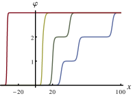
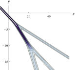
Figure 3: Plots of a solution of the scalar Burgers equation (7.1), with $\alpha=1$, at four different values ($-20,-10,-4,10$) of $y$. It is obtained from (7.3) with $n=3$, $\lambda_{1}=1$, $\lambda_{2}=2$, $\lambda_{3}=3$, and $\gamma_{1}=-10$, $\gamma_{2}=0$, $\gamma_{3}=10$. Evolution in the variable $y$ is from right to left. For large negative $y$, this is a $3$-kink solution (right curve). It then turns into a single kink and finally evolves into a shock wave (left curve). The second figure shows a contour plot of $\varphi_{x}$, which has the form of a rooted binary tree.

7.1.2 Darboux transformations

The following is obtained from Corollary 3.6. Setting $\boldsymbol{\alpha}=\boldsymbol{\beta}=0$ and $\boldsymbol{P}=\boldsymbol{Q}=-\partial_{x}$, we have to consider the following equations,

$$\alpha\,\boldsymbol{U}_{y}-\boldsymbol{U}_{xx}=\varphi_{0,x}\,\boldsymbol{U}\,,\qquad\boldsymbol{V}_{x}=-\boldsymbol{V}\,\varphi_{0}\,,\qquad\alpha\,\boldsymbol{V}_{y}=-\boldsymbol{V}\,\varphi_{0}^{2}\,,$$

$$\boldsymbol{X}_{x}=\boldsymbol{V}\,\boldsymbol{U}\,,\qquad\alpha\,\boldsymbol{X}_{y}=\boldsymbol{V}\boldsymbol{U}_{x}-\boldsymbol{V}_{x}\,\boldsymbol{U}\,.$$

The last two equations are solved by

$$\boldsymbol{X}=\boldsymbol{C}+\int\Big{(}\boldsymbol{V}\,\boldsymbol{U}\,dx+\frac{1}{\alpha}(\boldsymbol{V}\boldsymbol{U}_{x}-\boldsymbol{V}_{x}\,\boldsymbol{U})\,dy\Big{)}\,,$$ (7.4)

where $\boldsymbol{C}$ is constant and the integration is along any path from a fixed point $(x_{0},y_{0})$ to $(x,y)$. Then $\varphi=\varphi_{0}+\boldsymbol{U}\boldsymbol{X}^{-1}\boldsymbol{V}$ solves the Burgers equation (7.1).

Remark 7.2.

In the scalar case (i.e., $m=1$), we have

$$\varphi-\varphi_{0}=\boldsymbol{U}\boldsymbol{X}^{-1}\boldsymbol{V}=\mathrm{tr}(\boldsymbol{V}\boldsymbol{U}\boldsymbol{X}^{-1})=\mathrm{tr}(\boldsymbol{X}_{x}\boldsymbol{X}^{-1})=(\ln\det\boldsymbol{X})_{x}\,.$$

Expressing the seed solution as $\varphi_{0}=(\ln\Phi_{0})_{x}$ and setting $\Phi=\Phi_{0}\,\det\boldsymbol{X}$, we find

$$\alpha\,\Phi_{y}-\Phi_{xx}=(\alpha\,\Phi_{0,y}-\Phi_{0,xx})\,\Phi-2\,\Phi_{0}\,\Big{(}\mathrm{tr}(\boldsymbol{U}\boldsymbol{X}^{-1}\boldsymbol{V})\,\varphi_{0}+\mathrm{tr}(\boldsymbol{U}\boldsymbol{X}^{-1}\boldsymbol{V}_{x})\Big{)}\,,$$

which vanishes by use of $\boldsymbol{V}_{x}=-\boldsymbol{V}\,\varphi_{0}$ and if $\Phi_{0}$ satisfies (7.2). Hence $\Phi$ solves (7.2) and we expressed the Darboux transformation as a Cole-Hopf transformation.

Example 7.3.

If the seed solution $\varphi_{0}$ vanishes, $\boldsymbol{V}$ has to be constant and it only remains to solve $\alpha\,\boldsymbol{U}_{y}-\boldsymbol{U}_{xx}=0$. In the scalar case, writing $\boldsymbol{U}=(u_{1},\ldots,u_{n})$ and $\boldsymbol{V}=(v_{1},\ldots,v_{n})^{\intercal}$, for vanishing seed we find $u_{i}=a_{i}\,e^{\lambda_{i}\,x+\lambda_{i}^{2}\,y/\alpha}$, with constants $a_{i},\lambda_{i}$, and $\boldsymbol{X}_{ij}=\boldsymbol{C}_{ij}+v_{i}\,u_{j}/\lambda_{j}$. If $\boldsymbol{C}$ is invertible, we obtain the same solution $\varphi$ with $\boldsymbol{C}=\boldsymbol{I}$ and a redefined $\boldsymbol{V}$. Computing $\det\boldsymbol{X}$ via Sylvester’s determinant theorem and setting $a_{i}v_{i}/\lambda_{i}=:e^{\gamma_{i}}$, yields (7.3).

7.2 The second equation of the Burgers hierarchy

Now we extend $\mathcal{A}_{0}$ to the algebra of matrices of smooth functions of variables $x,y$ and $t$, and we set

$$\mathrm{d}f=\frac{1}{2}\,[\alpha\,\partial_{y}+\partial_{x}^{2},f]\,,\qquad\bar{\mathrm{d}}f=\frac{1}{3}\,[\partial_{t}-\partial_{x}^{3},f]\,.$$

Writing again $\phi=-\partial_{x}+\varphi$, and assuming that $\varphi$ is a matrix of functions, (1.1) splits into (7.1) and

$$\frac{1}{3}\,(\varphi_{t}-\varphi_{xxx})-\frac{1}{2}\,\varphi_{xx}\,\varphi-(\varphi_{x})^{2}-\frac{\alpha}{2}\,\varphi_{y}\,\varphi=0\,.$$

Using (7.1) in the last equation, converts the latter into the second member of a matrix Burgers hierarchy,

$$\varphi_{t}-\varphi_{xxx}-3\,(\varphi_{x}\,\varphi)_{x}-3\,\varphi_{x}\,\varphi^{2}=0\,.$$ (7.5)

We should stress that, though (1.1) is only a single equation for $\phi$, in terms of $\varphi$ it consists of two equations (which arise as the coefficients of $\partial_{x}^{0}$ and $\partial_{x}^{1}$), and these are equivalent to the first two equations of the Burgers hierarchy.

Setting $\phi_{0}=-\partial_{x}$ and $\gamma=0$, (2.1) is the Cole-Hopf transformation and (2.3) is equivalent to (7.2) and the second member of a matrix heat hierarchy, $\Phi_{t}-\Phi_{xxx}=0$.

7.3 KP

Let us now choose $\Omega$ according to (3.8) with $K=2$. We combine the above two bidifferential calculi, associated with the first two members of a matrix Burgers hierarchy, to

$$\mathrm{d}f=[\partial_{x},f]\,\xi_{1}+\frac{1}{2}\,[\alpha\partial_{y}+\partial_{x}^{2},f]\,\xi_{2}\,,\qquad\bar{\mathrm{d}}f=\frac{1}{2}\,[\alpha\partial_{y}-\partial_{x}^{2},f]\,\xi_{1}+\frac{1}{3}\,[\partial_{t}-\partial_{x}^{3},f]\,\xi_{2}\,.$$ (7.6)

With $\phi=-\partial_{x}+\varphi$, (1.1) is then equivalent to (7.1) and (7.5). Now (1.3) holds, and the integrability condition (1.4) turns out to be the matrix potential KP equation

$$\left(-4\varphi_{t}+\varphi_{xxx}+6(\varphi_{x})^{2}\right)_{x}+3\alpha^{2}\varphi_{yy}-6\alpha\,[\varphi_{x},\varphi_{y}]=0$$ (7.7)

(also see [12]). We recover the well-known fact that any solution of the first two members of the (matrix) Burgers hierarchy solves the (matrix) potential KP equation (see [24] and the references cited there). This is simply a special case of the implication (1.1) $\Rightarrow$ (1.4).

The resulting class of solutions of the scalar KP-II equation (with $\alpha=1$) for the variable $u=\varphi_{x}$, corresponding to the above class of multi-kink solutions of the Burgers equation, consists of KP line soliton solutions that form, at any time $t$, a rooted (and generically binary) tree-like structure in the $xy$-plane (see Fig. 3 for an example). An analysis (in a ‘tropical limit’) of this class of KP-II solutions has been carried out in [52, 53]. More complicated line soliton solutions of the scalar KP-II equation are obtained from $n\times n$ matrix Burgers equations via Corollary 3.5. But according to Remark 3.4, these solutions can be obtained in a simpler way from Theorem 3.1, with constant $\boldsymbol{P}$ and $\boldsymbol{Q}$. The resulting class of line-soliton solutions is well-known.

Proposition 7.4.

Let $\varphi_{0}$ be a constant $m\times m$ matrix, and $\tilde{\boldsymbol{P}}$ and $\tilde{\boldsymbol{Q}}$ solutions of the following $n\times n$ matrix equations

$$\alpha\tilde{\boldsymbol{P}}_{y}=\tilde{\boldsymbol{P}}_{xx}+2\,\tilde{\boldsymbol{P}}_{x}\,\tilde{\boldsymbol{P}}\,,\qquad\;\;\tilde{\boldsymbol{P}}_{t}=\tilde{\boldsymbol{P}}_{xxx}+3\,\tilde{\boldsymbol{P}}_{xx}\,\tilde{\boldsymbol{P}}+3\,\tilde{\boldsymbol{P}}_{x}\,\tilde{\boldsymbol{P}}^{2}+3\,\tilde{\boldsymbol{P}}_{x}^{2}\,,$$

$$\alpha\tilde{\boldsymbol{Q}}_{y}=-\tilde{\boldsymbol{Q}}_{xx}+2\,\tilde{\boldsymbol{Q}}\,\tilde{\boldsymbol{Q}}_{x}\,,\qquad\tilde{\boldsymbol{Q}}_{t}=\tilde{\boldsymbol{Q}}_{xxx}-3\,\tilde{\boldsymbol{Q}}\,\tilde{\boldsymbol{Q}}_{xx}+3\,\tilde{\boldsymbol{Q}}^{2}\tilde{\boldsymbol{Q}}_{x}-3\,\tilde{\boldsymbol{Q}}_{x}^{2}\,,$$

which are the first two members of two versions of a matrix Burgers hierarchy. Let $\boldsymbol{X}$ be an invertible solution of the system of linear ordinary differential equations

$$\boldsymbol{X}_{x} = \boldsymbol{V}_{0}\,\boldsymbol{U}_{0}+\tilde{\boldsymbol{Q}}\,\boldsymbol{X}-\boldsymbol{X}\,\tilde{\boldsymbol{P}}\,,$$

$$\alpha\boldsymbol{X}_{y} = \tilde{\boldsymbol{Q}}\,\boldsymbol{V}_{0}\,\boldsymbol{U}_{0}+\boldsymbol{V}_{0}\,\boldsymbol{U}_{0}\,\tilde{\boldsymbol{P}}-(\tilde{\boldsymbol{Q}}_{x}-\tilde{\boldsymbol{Q}}^{2})\,\boldsymbol{X}-\boldsymbol{X}\,(\tilde{\boldsymbol{P}}_{x}+\tilde{\boldsymbol{P}}^{2})\,,$$

$$\boldsymbol{X}_{t} = \tilde{\boldsymbol{Q}}\,\boldsymbol{V}_{0}\,\boldsymbol{U}_{0}\,\tilde{\boldsymbol{P}}-(\tilde{\boldsymbol{Q}}_{x}-\tilde{\boldsymbol{Q}}^{2})\,\boldsymbol{V}_{0}\,\boldsymbol{U}_{0}+\boldsymbol{V}_{0}\,\boldsymbol{U}_{0}\,(\tilde{\boldsymbol{P}}_{x}+\tilde{\boldsymbol{P}}^{2})$$

$$+(\tilde{\boldsymbol{Q}}_{xx}-\tilde{\boldsymbol{Q}}_{x}\,\tilde{\boldsymbol{Q}}-2\,\tilde{\boldsymbol{Q}}\,\tilde{\boldsymbol{Q}}_{x}+\tilde{\boldsymbol{Q}}^{3})\,\boldsymbol{X}-\boldsymbol{X}\,(\tilde{\boldsymbol{P}}_{xx}+\tilde{\boldsymbol{P}}\,\tilde{\boldsymbol{P}}_{x}+2\,\tilde{\boldsymbol{P}}_{x}\,\tilde{\boldsymbol{P}}+\tilde{\boldsymbol{P}}^{3})\,,$$

with any constant matrices $\boldsymbol{U}_{0}$, $\boldsymbol{V}_{0}$, of size $m\times n$, respectively $n\times m$. Then $\varphi=\varphi_{0}+\boldsymbol{U}_{0}\,\boldsymbol{X}^{-1}\boldsymbol{V}_{0}$ solves the $m\times m$ matrix potential KP equation (7.7).

Proof.

This is obtained from Corollary 3.5, using (7.6) and setting $\boldsymbol{P}=\tilde{\boldsymbol{P}}-\partial_{x}$, $\boldsymbol{Q}=\tilde{\boldsymbol{Q}}-\partial_{x}$, $\boldsymbol{\alpha}=\boldsymbol{\beta}=0$. ∎

Remark 7.5.

Proposition 7.4 is more of structural interest than of practical use. Reducing the matrix Burgers hierarchy equations to heat hierarchy equations via Cole-Hopf transformations,

$$\tilde{\boldsymbol{P}}=\boldsymbol{\Phi}_{x}\,\boldsymbol{\Phi}^{-1}\,,\qquad\;\;\,\alpha\boldsymbol{\Phi}_{y}=\boldsymbol{\Phi}_{xx}\,,\qquad\boldsymbol{\Phi}_{t}=\boldsymbol{\Phi}_{xxx}\,,$$

$$\tilde{\boldsymbol{Q}}=-\boldsymbol{\Psi}^{-1}\boldsymbol{\Psi}_{x}\,,\qquad\alpha\boldsymbol{\Psi}_{y}=-\boldsymbol{\Psi}_{xx}\,,\quad\boldsymbol{\Psi}_{t}=\boldsymbol{\Psi}_{xxx}\,,$$

in terms of ${\boldsymbol{U}}:=\boldsymbol{U}_{0}\boldsymbol{\Phi}$ and ${\boldsymbol{V}}:=\boldsymbol{\Psi}\boldsymbol{V}_{0}$, the solution of the equations for $\boldsymbol{X}$ can be expressed as

$$\boldsymbol{X}=\boldsymbol{\Psi}^{-1}\Big{(}\boldsymbol{C}+\int_{(x_{0},y_{0},t_{0})}^{(x,y_{0},t_{0})}\boldsymbol{V}\boldsymbol{U}\,dx+\alpha^{-1}\int_{(x,y_{0},t_{0})}^{(x,y,t_{0})}(\boldsymbol{V}\boldsymbol{U}_{x}-\boldsymbol{V}_{x}\,\boldsymbol{U})\,dy$$

$$+\int_{(x,y,t_{0})}^{(x,y,t)}(\boldsymbol{V}_{xx}\,\boldsymbol{U}-\boldsymbol{V}_{x}\,\boldsymbol{U}_{x}+\boldsymbol{V}\boldsymbol{U}_{xx})\,dt\Big{)}\,\boldsymbol{\Phi}^{-1}\,,$$

with a constant matrix $\boldsymbol{C}$. This expression generalizes (7.4). Now one only has to solve linear (matrix) heat hierarchy equations in order to construct solutions of the KP equation. There are quite a number of previous results about matrix solutions of the KP equation and its hierarchy, see [54], for example.

Of course, all this can be extended to the whole matrix KP hierarchy, see [12] for a corresponding bidifferential calculus.

8 Matrix Davey-Stewartson system

8.1 Another ‘Riemann equation’

Let $\mathcal{B}_{0}$ be the space of smooth complex functions on $\mathbb{R}^{2}$. We extend it to $\mathcal{B}=\mathcal{B}_{0}[\partial_{x}]$, where $\partial_{x}=\partial/\partial x$. On $\mathrm{Mat}(m,m,\mathcal{B})$ we define

$$\mathrm{d}f=[J,f]\,,\qquad\bar{\mathrm{d}}f=[\partial_{y}-J\partial_{x},f]\,,$$ (8.1)

where $J\neq I$ is a constant $m\times m$ matrix. Then (1.1) becomes

$$\phi_{y}=[J\partial_{x},\phi]+[J,\phi]\,\phi=J\,\phi_{x}+[J,\phi]\,(\phi+\partial_{x})\,.$$ (8.2)

This suggests to introduce a new dependent variable $\varphi$ via

$$\phi=J\,\varphi-\partial_{x}\,,$$ (8.3)

in order to eliminate explicit operator terms. Assuming $J^{2}=I$, (8.2) reads

$$\varphi_{y}=J\,\varphi_{x}+[J,\varphi]\,J\varphi\,,$$ (8.4)

where $\varphi$ can now be restricted to be a matrix over $\mathcal{B}_{0}$. We choose $J$ and decompose $\varphi$ as in (6.9). The last equation then splits into

$$u_{y}-u_{x}+2qr=0\,,\quad v_{y}+v_{x}+2rq=0\,,\quad q_{y}-q_{x}+2qv=0\,,\quad r_{y}+r_{x}+2ru=0\,.$$ (8.5)

A Cole-Hopf transformation for this system is obtained according to Section 2. The explicit operator term that arises in (2.1) via the substitution (8.3) is eliminated by setting $\phi_{0}=-\partial_{x}$. Then (2.1) becomes

$$\varphi=J\,(\phi+\partial_{x})=-J\Phi\partial_{x}\Phi^{-1}+J\partial_{x}=J\Phi_{x}\Phi^{-1}\,,$$ (8.6)

Using (8.1), (2.3) with $\gamma=0$ reads

$$\Phi_{y}-J\Phi_{x}=0\,.$$ (8.7)

All solutions of (8.4) can be reached in this way. Writing

$$\Phi=\left(\begin{array}[]{cc}f_{1}&f_{2}\\ g_{1}&g_{2}\end{array}\right)\,,$$

(8.7) means that, for $i=1,2$, $f_{i}$ ($g_{i}$) only depends on $\tilde{x}$ ($\tilde{y}$), where

$$\tilde{x}=x+y\,,\qquad\tilde{y}=x-y\,.$$ (8.9)

Using $\partial_{\tilde{x}}:=\frac{1}{2}(\partial_{x}+\partial_{y})$, $\partial_{\tilde{y}}:=\frac{1}{2}(\partial_{x}-\partial_{y})$, the system (8.5) can actually be expressed in a more compact form. But in Section 8.2 we will supplement (8.5) by further equations that are not conveniently expressed in terms of these new variables. Therefore we will not pass over to them, except in Section 8.1.1, where it achieves a substantial simplification.

Next we implement the Hermitian conjugation reductions (6.13) with $C=\mbox{block-diag}(C_{1},C_{2})$, where $C_{1}$ and $C_{2}$ are constant anti-Hermitian matrices. This generalization of the naive reduction conditions $\varphi^{\dagger}=\varphi$, respectively $\varphi^{\dagger}=J\varphi J$, by introduction of the matrix $C$, is important in order to recover relevant solutions of the DS equation from its ‘Riemann system’ (see Section 8.2). The reduction conditions are equivalent to

$$r=\mu\,q^{\dagger}\,,\qquad u=u^{\dagger}+C_{1}\,,\qquad v=v^{\dagger}+C_{2}\,,\qquad$$ (8.10)

where $\mu=-1$ ($\mu=1$) corresponds to the focusing (defocusing) case in (6.13). This reduces (8.5) to

$$u_{y}-u_{x}+2\mu\,qq^{\dagger}=0\,,\quad v_{y}+v_{x}+2\mu\,q^{\dagger}q=0\,,\quad q_{y}-q_{x}+2qv=0\,,\quad q_{y}+q_{x}+2u^{\dagger}q=0\,.$$ (8.11)

Using (8.6), we obtain the following translation of the reductions conditions (6.13),

$$\varphi^{\dagger}=\varphi+C \Longleftrightarrow \Phi^{\dagger}_{x}J\Phi=\Phi^{\dagger}J\Phi_{x}+\Phi^{\dagger}C\Phi$$

$$\varphi^{\dagger}=J\,\varphi\,J+C \Longleftrightarrow \Phi^{\dagger}_{x}\Phi=\Phi^{\dagger}\Phi_{x}+\Phi^{\dagger}CJ\Phi\,.$$ (8.12)

These are nonlinear ordinary differential equations for $\Phi$, so that the reduction conditions are difficult to implement on the level of the Cole-Hopf transformation. However, at least in the scalar case ($m_{1}=m_{2}=1$ in (6.9)), this problem can be solved completely, as shown below.

8.1.1 Cole-Hopf transformation in the scalar case

We use the coordinates (8.9). In the scalar case ($m_{1}=m_{2}=1$), writing

$$f_{i}(\tilde{x})=F_{i}(\tilde{x})\,e^{\mathrm{i}c\,\tilde{x}}\,,\qquad g_{i}(\tilde{y})=G_{i}(\tilde{y})\,e^{-\mathrm{i}\tilde{c}\,\tilde{y}}\,,$$

with $c:=\frac{1}{2}\mathrm{i}C_{1}$ and $\tilde{c}:=\frac{1}{2}\mathrm{i}C_{2}$, reduces (8.12) to the Wronskian conditions

$$\left|\begin{array}[]{cc}F_{1}&F_{2}\\ F_{1}^{\prime}&F_{2}^{\prime}\end{array}\right|=\alpha\,,\quad\left|\begin{array}[]{cc}G_{1}&G_{2}\\ G_{1}^{\prime}&G_{2}^{\prime}\end{array}\right|=\mu\,\alpha\,,$$ (8.17)

where $\alpha\in\mathbb{R}\setminus\{0\}$, a prime denotes a derivative with respect to the argument, and the functions $F_{i},G_{i}$ have to be real. (8.6) leads to

$$q=\alpha\,F^{-1}\,e^{\mathrm{i}c\,\tilde{x}+\mathrm{i}\tilde{c}\,\tilde{y}}\,,\quad u=(\ln F)_{\tilde{x}}+\mathrm{i}\,c\,,\quad v=-(\ln F)_{\tilde{y}}+\mathrm{i}\,\tilde{c}\,,$$

where

$$F(\tilde{x},\tilde{y}):=F_{1}(\tilde{x})\,G_{2}(\tilde{y})-F_{2}(\tilde{x})\,G_{1}(\tilde{y})\,.$$

Example 8.1.

Choosing

$$f_{i}=a_{i}\,e^{\theta}+b_{i}\,e^{-\theta^{\ast}}\,,\quad g_{i}=c_{i}\,e^{\tilde{\theta}}+d_{i}\,e^{-\tilde{\theta}^{\ast}}\,,\quad i=1,2\,,\qquad\theta:=\lambda\,\tilde{x}\,,\qquad\tilde{\theta}:=\tilde{\lambda}\,\tilde{y}\,,$$

with real constants $a_{i},b_{i},c_{i},d_{i}$, and complex constants $\lambda$, $\tilde{\lambda}$, with $\mathrm{Im}(\lambda)=c$ and $\mathrm{Im}(\tilde{\lambda})=-\tilde{c}$, the above Wronskian conditions are solved with $\alpha=-2\mathrm{Re}(\lambda)\,(a_{1}b_{2}-a_{2}b_{1})$. An asterisk denotes complex conjugation. From (8.6) we obtain

$$q = \frac{\alpha}{\Delta}\,e^{\mathrm{i}\,\mathrm{Im}(\theta-\tilde{\theta})}\,,\quad r=\frac{\beta}{\Delta}\,e^{\mathrm{i}\,\mathrm{Im}(\tilde{\theta}-\theta)}\,,$$

$$u = \mathrm{i}\,\mathrm{Im}(\lambda)+\mathrm{Re}(\lambda)\,\frac{\Delta_{1}+\Delta_{2}}{\Delta}\,,\quad v=-\mathrm{i}\,\mathrm{Im}(\tilde{\lambda})+\mathrm{Re}(\lambda)\,\frac{\Delta_{1}-\Delta_{2}}{\Delta}\,,$$

where we set $\beta:=-2\mathrm{Re}(\tilde{\lambda})\,(c_{1}d_{2}-c_{2}d_{1})$ and

$$\Delta_{1} := (a_{1}d_{2}-a_{2}d_{1})\,e^{\mathrm{Re}(\theta-\tilde{\theta})}-(b_{1}c_{2}-b_{2}c_{1})\,e^{\mathrm{Re}(\tilde{\theta}-\theta)}\,,$$

$$\Delta_{2} := (a_{1}c_{2}-a_{2}c_{1})\,e^{\mathrm{Re}(\theta+\tilde{\theta})}-(b_{1}d_{2}-b_{2}d_{1})\,e^{-\mathrm{Re}(\theta+\tilde{\theta})}\,,$$

$$\Delta := \Delta_{1}+\Delta_{2}+2\,(b_{1}d_{2}-b_{2}d_{1})\,e^{-\mathrm{Re}(\theta+\tilde{\theta})}+2\,(b_{1}c_{2}-b_{2}c_{1})\,e^{\mathrm{Re}(\tilde{\theta}-\theta)}\,.$$

This provides us with solutions of the reduction conditions (8.11) if $\beta=\mu\,\alpha$, i.e.,

$$\mathrm{Re}(\tilde{\lambda})=\mu\,\frac{a_{1}b_{2}-a_{2}b_{1}}{c_{1}d_{2}-c_{2}d_{1}}\mathrm{Re}(\lambda)\,,$$ (8.18)

assuming $a_{1}b_{2}\neq a_{2}b_{1}$ and $c_{1}d_{2}\neq c_{2}d_{1}$. A solution from the above family is regular iff $\Delta$ is everywhere different from zero. This is so if one of the coefficients of the sum of exponentials is positive and all others greater or equal to zero.

Remark 8.2.

In the scalar case, the system (8.11) has the following consequences,

$$(\ln q)_{\tilde{x}\tilde{y}}=-\mu\,|q|^{2}\,,\qquad\left(u_{\tilde{x}}+\mathrm{Re}(u^{2})\right)_{\tilde{y}}=0\,,\qquad\left(v_{\tilde{x}}-\mathrm{Re}(u^{2})\right)_{\tilde{y}}=0\,.$$

In terms of $w:=\ln q$, the first becomes a Liouville equation. The last two equations can be integrated to first order equations. The solutions of (8.11) obtained above also solve these equations.

8.2 ‘Riemann system’ associated with the matrix Davey-Stewartson system

Let now $\mathcal{B}$ be the space of smooth complex functions on $\mathbb{R}^{3}$. We extend (8.1) as follows,

$$\mathrm{d}f=[J,f]\,\xi_{1}+[\partial_{y}+J\partial_{x},f]\,\xi_{2}\,,\qquad\bar{\mathrm{d}}f=[\partial_{y}-J\partial_{x},f]\,\xi_{1}-[\mathrm{i}\,\partial_{t}+J\partial_{x}^{2},\,f]\,\xi_{2}\,.$$ (8.19)

In terms of $\varphi$ given by (8.3), (1.1) is equivalent to (8.4), where $\varphi$ is now allowed to also depend on $t$, together with

$$\mathrm{i}\,\varphi_{t}=-J\varphi_{xx}-\varphi_{y}J\varphi-J\,\varphi_{x}J\varphi-[J,\varphi]J\varphi_{x}\,.$$ (8.20)

These two equations constitute the ‘Riemann system’ for

$$-{\mathrm{i}}\,[J,\varphi_{t}]=\varphi_{yy}-J\varphi_{xx}J+J[\varphi_{x}+J\varphi_{y},J[J,\varphi]]-J[J,\varphi]\,[J,\varphi_{x}]\,,$$ (8.21)

which results from (1.4). (8.20) decomposes into which results from (1.4). (8.20) decomposes into

$$\mathrm{i}q_{t}=-q_{xx}+q_{y}v-u_{y}q+q_{x}v-u_{x}q+2qv_{x}\,,$$

$$\mathrm{i}r_{t}=r_{xx}+v_{y}r-r_{y}u+r_{x}u-v_{x}r+2ru_{x}\,,$$

$$\mathrm{i}u_{t}=-u_{xx}+q_{y}r-u_{y}u+q_{x}r-u_{x}u+2qr_{x}\,,$$

$$\mathrm{i}v_{t}=v_{xx}+v_{y}v-r_{y}q+r_{x}q-v_{x}v+2rq_{x}\,.$$

Implementing the reduction conditions (8.10), this becomes

$$\mathrm{i}q_{t}=-q_{xx}+q_{y}v-u_{y}q+q_{x}v-u_{x}q+2qv_{x}\,,$$

$$\mathrm{i}u_{t}=-u_{xx}+\mu q_{y}q^{\dagger}-u_{y}u+\mu q_{x}q^{\dagger}-u_{x}u+2\mu qq^{\dagger}_{x}\,,$$ (8.22)

$$\mathrm{i}v_{t}=v_{xx}+v_{y}v-\mu q^{\dagger}_{y}q+\mu q^{\dagger}_{x}q-v_{x}v+2\mu q^{\dagger}q_{x}\,,$$

$$(qv)_{y}+(qv)_{x}+u_{x}q-u_{y}q-u^{\dagger}q_{y}+u^{\dagger}q_{x}=0\,.$$

The last equation of (8.22) is a consequence of (8.11). Using the change of variables $\tilde{u}:=u_{y}+u_{x}$, $\tilde{v}:=v_{y}-v_{x}$, and (6.9), we decompose (8.21) into

$$2\mathrm{i}\,q_{t}\,+q_{xx}+q_{yy}+2\,(q\tilde{v}\,+\,\tilde{u}q)=0\,, \tilde{u}_{x}-\tilde{u}_{y}=2\,\left((qr)_{x}+(qr)_{y}\right)\,,$$

$$-2\mathrm{i}\,r_{t}+r_{xx}+r_{yy}+2\,(r\tilde{u}+\tilde{v}r)=0\,, \tilde{v}_{x}+\tilde{v}_{y}=2\,\left((rq)_{x}-(rq)_{y}\right)\,.$$ (8.23)

The reduction conditions (8.10) imply

$$r=\mu\,q^{\dagger}\,,\qquad\tilde{u}=\tilde{u}^{\dagger}\,,\qquad\tilde{v}=\tilde{v}^{\dagger}\,.$$

This reduces (8.23) to

$$2\mathrm{i}\,q_{t}+q_{xx}+q_{yy}+2(q\,\tilde{v}+\tilde{u}\,q)=0\,,$$

$$\tilde{u}_{x}-\tilde{u}_{y}=2\mu\left((qq^{\dagger})_{x}+(qq^{\dagger})_{y}\right)\,,\qquad\tilde{v}_{x}+\tilde{v}_{y}=2\mu\left((q^{\dagger}q)_{x}-(q^{\dagger}q)_{y}\right)\,,$$ (8.24)

which is a matrix version [55, 56, 57, 24, 58, 59] of the Davey-Stewartson (DS) equation [60]. (8.11) and (8.22) constitute the associated ‘Riemann system’, which is quite involved. Any solution of it is also a solution of the DS system (8.24). According to Section 2, the Cole-Hopf transformation in Section 8.1 extends to the present ‘Riemann system’, if we add the equation

$$\mathrm{i}\,\Phi_{t}+J\Phi_{xx}=0\,.$$ (8.25)

Example 8.3.

We extend Example 8.1. Now the functions $f_{i}$ and $g_{i}$ also depend on $t$, and (8.25) leads to the additional equations

$$\mathrm{i}f_{j,t}+f_{j,xx}=0\,,\qquad\mathrm{i}g_{j,t}-g_{j,xx}=0\,.$$

In the solutions presented in Example 8.1, we then simply have to make the substitutions

$$\theta\mapsto\lambda\,(x+y)+\mathrm{i}\lambda^{2}\,t\,,\qquad\tilde{\theta}\mapsto\tilde{\lambda}\,(x-y)-\mathrm{i}\tilde{\lambda}^{2}\,t\,.$$

In this way we recover solutions of the scalar DS system (8.24), with $\mu=-1$, in a similar form as presented in [17]. We have a single dromion solution if $a_{1}c_{2}-a_{2}c_{1}>0$, $b_{1}d_{2}-b_{2}d_{1}>0$, $b_{1}c_{2}-b_{2}c_{1}>0$, and $a_{1}d_{2}-a_{2}d_{1}>0$. This degenerates to a single solitoff solution if $a_{1}c_{2}-a_{2}c_{1}=0$, which in turn degenerates to a single soliton solution if $b_{1}d_{2}-b_{2}d_{1}=0$. In all these cases, also (8.18), with $\mu=-1$, has to hold.

9 Concluding and further remarks

In this work we explored realizations of the ‘Riemann equation’ (1.1) (or (1.2)) in bidifferential calculus. The most basic examples are the matrix Riemann equation, and a semi- and a full discretization of it. These integrable discretizations are easily obtained in bidifferential calculus from the continuous case, essentially by replacing in the expressions for $\mathrm{d}$ and $\bar{\mathrm{d}}$ a commutator with a partial derivative operator by a commutator with a shift operator. This works correspondingly for continuous, semi- and fully discrete matrix NLS equations [49].

The semi-discrete Riemann equation (4.4) appeared in [26] (see (3.23) therein) as an ‘infinitesimal symmetry’ (analog of infinitesimal Lie point symmetry) of the discrete Burgers equation (4.25), in the scalar case. The (fully) discrete Riemann equation (4.12) is a corresponding ‘finite symmetry’ of the discrete Burgers equation. Furthermore, it can be easily verified that the semi-discrete Riemann equation (4.4) and the discrete Riemann equation (4.13) are compatible. More generally, the semi-discrete Riemann hierarchy and the (fully) discrete Riemann hierarchy form a common hierarchy. This can be concluded from the fact that they share the same Cole-Hopf formula (4.5) (cf. (4.14)), and the corresponding linear equations are compatible.

Another point we concentrated on in this work is the implication (1.9). Special cases are the relation between the Burgers and the KP hierarchy (Section 7), as well as an observation made in case of the sdYM equation in [10], see Section 5.1. From the bidifferential calculus generalization it is clear that behind this is in fact a common and general feature, so there are counterparts in case of other integrable equations. We demonstrated this for (matrix versions of) the two-dimensional Toda lattice, a variant of Hirota’s bilinear difference equation, (2+1)-dimensional NLS and DS equations.

If a ‘Riemann system’ involves a Riemann equation, perhaps via a reduction, we may expect to obtain a ‘breaking soliton’ case in the sense, e.g., of Bogoyavlenskii’s work (see [22, 30], in particular). Here the sdYM equation is the prime example. In the case of the (2+1)-dimensional NLS equation, the resulting solutions are actually singular, rather than just ‘breaking’.

In contrast to the Riemann equation, the integrable discrete versions possess infinite families of regular solutions that describe multi-kinks. The appearance of very much the same families of solutions of seemingly quite different, integrable equations, like discrete Riemann equations, Toda, Hirota-Miwa, Burgers and KP equations, is traced back to simple relations between the associated ‘Riemann equations’.

Our results suggest that any integrable equation, which is not already either C-integrable (so that there is a kind of Cole-Hopf transformation, cf. [14, 15, 16]) or integrable via a hodograph method, or perhaps a combination of both, contains a subset of solutions that are the solutions of a system of equations which is integrable in this more special sense.

In the examples presented in this work, we may think of exchanging $\mathrm{d}$ and $\bar{\mathrm{d}}$ in (1.1) to get further integrable equations. However, a simple computation, using the Leibniz rule, shows that

$$\bar{\mathrm{d}}\phi-(\mathrm{d}\phi)\,\phi=0\quad\Longleftrightarrow\quad\mathrm{d}\phi^{-1}-(\bar{\mathrm{d}}\phi^{-1})\,\phi^{-1}=0\,,$$ (9.1)

assuming that $\phi$ has an inverse. A corresponding statement also holds for (1.5):

$$\mathrm{d}[(\bar{\mathrm{d}}g)\,g^{-1}]=0\quad\Longleftrightarrow\quad\bar{\mathrm{d}}[(\mathrm{d}g^{-1})\,g]=0\,.$$

In contrast, in case of (1.4) an exchange of $\mathrm{d}$ and $\bar{\mathrm{d}}$ can lead to an inequivalent equation (cf. Section 5.3). In particular, it may relate a member of a hierarchy with a member of a corresponding ‘negative’ or ‘reciprocal’ hierarchy, see [61]. (9.1) shows that the corresponding ‘Riemann systems’ are simply related via $\phi\mapsto\phi^{-1}$.

The ‘linearization method’ of Section 2, if applicable to a ‘Riemann system’, does not extend to the respective realizations of (1.4) or (1.5). But the binary Darboux transformation theorem (see Section 3) applies to them and quickly leads to infinite (soliton-type) families of explicit solutions. This will be elaborated further in a follow-up work. In the present work we demonstrated that the binary Darboux transformation method also makes sense for ‘Riemann systems’. Needless to say, the list of examples presented in this work can easily be extended.

We should also emphasize the special case of Theorem 3.1, formulated in Corollary 3.5. If the seed solution satisfies $\mathrm{d}\phi_{0}=0$, and if the bidifferential calculus extends to second order, this expresses a way to generate solutions of (1.4) or (1.5) from solutions of $n\times n$ versions of the associated ‘Riemann system’, for arbitrary $n\in\mathbb{N}$. This includes a construction of breaking multi-soliton-type solutions of the sdYM equation (see the related work in [10]) and similar solutions of the (matrix) (2+1)-dimensional NLS equation.

It was not our aim in this work to obtain new integrable equations, but according to our knowledge the matrix version (4.25) of the fully discrete Burgers equation is new, and possibly also the integrable full discretization (4.13) of the Riemann equation (although this would be surprising). Moreover, this also concerns the generalization of Hirota’s bilinear difference equation obtained in Section 5.3.

A systematic search for equations possessing a bidifferential calculus formulation, with the help of computer algebra, has not yet been undertaken. It will lead to further examples.

Acknowledgments. O.C. would like to thank the Mathematical Institute of the University of Göttingen for hospitality in November 2013 - April 2014, when part of this work has been carried out. Special thanks go to Dorothea Bahns. Since October 2014, O.C. has been supported via an Alexander von Humboldt fellowship for postdoctoral researchers. N.S. has been supported by the Marie Curie Actions Intra-European fellowship HYDRON (FP7-PEOPLE-2012-IEF, Project number 332136). The authors are also grateful to Aristophanes Dimakis, for sharing some of his insights, and to Eugene Ferapontov and Maxim Pavlov for some very motivating discussions.

Appendix A: Volterra lattice equation

The alternative integrable semi-discretization

$$u_{t}=u^{+}\,u-u\,u^{-}$$ (1.1)

of the Riemann equation is known as the (Lotka-) Volterra lattice equation (see, e.g., [62]). In the scalar case, for positive solutions, writing $u=a^{2}$, it becomes the (integrable) Kac-VanMoerbeke lattice equation $a_{t}=a\,[(a^{+})^{2}-(a^{-})^{2}]$. (1.1) is a matrix version of the Volterra lattice equation. Though not as a realization of (1.1), a kind of potential version of it can be obtained as a realization of (1.4). Let us consider the bidifferential calculus given by

$$\mathrm{d}f=[\mathbb{S}^{r},f]\,\xi_{1}+[\mathbb{S},f]\,\xi_{2}\,,\qquad\bar{\mathrm{d}}f=f_{t}\,\xi_{1}+[\mathbb{S}^{1-r},f]\,\xi_{2}\,,$$

with some integer $r>1$. Setting $\phi=\varphi\,\mathbb{S}^{-r}$ in (1.4) yields

$$\varphi^{(1)}_{t}-\varphi_{t}=(\varphi^{(r)}-\varphi)(\varphi^{(1)}-\varphi-I)-(\varphi^{(1)}-\varphi-I)(\varphi^{(r)}-\varphi)^{(1-r)}\,,$$

where $\varphi^{(r)}=\mathbb{S}^{r}\varphi\mathbb{S}^{-r}$. In terms of $u:=\varphi^{(1)}-\varphi-I$, it takes the form

$$u_{t}=\sum_{i=1}^{r-1}u^{(i)}\,u-u\sum_{i=1-r}^{-1}u^{(i)}\,,$$

which for $r=2$ is (1.1) (cf. [12]). The associated ‘Riemann system’, obtained from (1.1), is

$$\varphi_{t}=(\varphi^{(r)}-\varphi)\,\varphi\,,\qquad\varphi^{(r)}=I+\varphi^{(r-1)}\,(I-\varphi^{-1})\,.$$

The first is the semi-discrete Riemann equation (4.2) (where $\mathbb{S}$ is replaced by $\mathbb{S}^{r}$), the second a recurrence relation.

References

- [1] D. Levi, O. Ragnisco, and M. Bruschi, “Continuous and discrete matrix Burgers’ hierarchies,” Nuovo Cimento B 74, 33–51 (1983).
- [2] O.I. Bogoyavlenskiĭ, “Breaking solitons. V. Systems of hydrodynamic type,” Math. USSR Izvestiya 38, 439–454 (1992).
- [3] E.V. Ferapontov, “On the matrix Hopf equation and integrable Hamiltonian systems of hydrodynamic type, which do not possess Riemann invariants,” Phys. Lett. A 179, 391–397 (1993).
- [4] E.V. Ferapontov, “Several conjectures and results in the theory of integrable Hamiltonian systems of hydrodynamic type, which do not possess Riemann invariants,” Theor. Math. Phys. 99, 567–570 (1994).
- [5] F. Guil, M. Mañas, and G. Álvarez, “The Hopf-Cole transformation and the KP equation,” Phys. Lett. A 190, 49–52 (1994).
- [6] K.T. Joseph and A.S. Vasudeva Murthy, “Hopf-Cole transformation to some systems of partial differential equations,” Nonlinear Diff. Equ. Appl. 8, 173–193 (2001).
- [7] D.J. Arrigo and F. Hickling, “Darboux transformations and linear parabolic partial differential equations,” J. Phys. A: Math. Gen. 35, L389–L399 (2002).
- [8] P.M. Santini and A.I. Zenchuk, “The general solution of the matrix equation ,” Phys. Lett. A 368, 48–52 (2007).
- [9] A.I. Zenchuk, “Matrix equations of hydrodynamic type as lower-dimensional reductions of self-dual type -integrable systems,” arXiv:0708.2050 (2007).
- [10] A.I. Zenchuk, “Lower-dimensional reductions of self-dual Yang-Mills equation: Solutions with break of wave profiles,” J. Math. Phys. 49, 063502 (2008).
- [11] A. Dimakis and F. Müller-Hoissen, “Bi-differential calculi and integrable models,” J. Phys. A: Math. Gen. 33, 957–974 (2000).
- [12] A. Dimakis and F. Müller-Hoissen, “Bidifferential graded algebras and integrable systems,” Discr. Cont. Dyn. Systems Suppl. 2009, 208–219 (2009).
- [13] A. Dimakis and F. Müller-Hoissen, “Binary Darboux transformations in bidifferential calculus and integrable reductions of vacuum Einstein equations,” SIGMA 9, 009 (31 pages) (2013).
- [14] F. Calogero and W. Eckhaus, “Nonlinear evolution equations, rescalings, model PDEs and their integrability. I,” Inv. Problems 3, 229–262 (1987).
- [15] F. Calogero, “-Integrable nonlinear partial differential equations. I,” J. Math. Phys. 32, 375–887 (1991).
- [16] F. Calogero, “-Integrable nonlinear partial differential equations in dimensions,” J. Math. Phys. 33, 1257–1271 (1992).
- [17] V.B. Matveev and M.A. Salle, Darboux Transformations and Solitons, Springer Series in Nonlinear Dynamics (Springer, Berlin, 1991).
- [18] V.B. Matveev, “Darboux transformations, covariance theorems and integrable systems,” in L.D. Faddeev’s Seminar on Mathematical Physics, edited by M.A. Semenov-Tian-Shansky, Vol. 201 of Advances in the Mathematical Sciences (AMS, Providence, R.I., 2000), 179–209.
- [19] A. Dimakis, N. Kanning, and F. Müller-Hoissen, “The non-autonomous chiral model and the Ernst equation of general relativity in the bidifferential calculus framework,” SIGMA 7, 118 (2011).
- [20] D. Maison, “Are the stationary, axially symmetric Einstein equations completely integrable?” Phys. Rev. Lett. 41, 521–522 (1978).
- [21] S.P. Burtsev, V.E. Zakharov, and A.V. Mikhailov, “Inverse scattering method with variable spectral parameter,” Theor. Math. Phys. 70, 227–240 (1987).
- [22] O.I. Bogoyavlenskiĭ, “Breaking solitons in -dimensional integrable equations,” Russ. Math. Surveys 45, 1–86 (1990).
- [23] P.A. Clarkson, P.R. Gordoa, and A. Pickering, “Multicomponent equations associated to non-isospectral scattering problems,” Inv. Problems 13, 1463–1476 (1997).
- [24] A. Dimakis and F. Müller-Hoissen, “Multicomponent Burgers and KP hierarchies, and solutions from a matrix linear system,” SIGMA 5, 002 (2009).
- [25] V.A. Belinskiǐ and V.E. Zakharov, “Integration of the Einstein equations by means of the inverse scattering problem technique and construction of exact soliton solutions,” Sov. Phys. JETP 48, 985–994 (1978).
- [26] R. Hernández Heredero, D. Levi, and P. Winternitz, “Symmetries of the discrete Burgers equation,” J. Phys. A: Math. Gen. 32, 2685–2695 (1999).
- [27] F. Calogero and A. Degasperis, “Nonlinear evolution equations solvable by the inverse spectral transform,” Il Nuovo Cim. B 32, 201–242 (1976).
- [28] V.E. Zakharov, “The inverse scattering method,” in Solitons, edited by R.K. Bullough and P.J. Caudrey, Vol. 17 of Topics in Current Physics (Springer, Berlin, 1980), 243–285.
- [29] I. Strachan, “A new family of integrable models in dimensions associated with Hermitian symmetric spaces,” J. Math. Phys. 33, 2477–2482 (1992).
- [30] O.I. Bogoyavlenskiĭ, “Breaking solitons. III,” Math. USSR Izvestiya 36, 129–137 (1991).
- [31] J.Z. Hearan, “Nonsingular solutions of ,” Lin. Alg. Appl. 16, 57–63 (1977).
- [32] V.B. Matveev and M.A. Salle, “Darboux transformation and two-dimensional Toda lattice,” Journal of Mathematical Sciences 23, 2441–2446 (1983).
- [33] X.-Y. Wen, Y.-T. Gao, Y.-S. Xue, R. Guo, F.-H. Qi, and X. Yu, “Integrable hierarchy covering the lattice Burgers equation in fluid mechanics: -fold Darboux transformation and conservation laws,” Commun. Theor. Phys. 58, 323–330 (2012).
- [34] E. Ben-Naim and S. Redner, “Dynamics of social diversity,” J. Stat. Mech. 2005, L11002 (2005).
- [35] A. Dimakis and F. Müller-Hoissen, “Functional representations of integrable hierarchies,” J. Phys. A: Math. Gen. 39, 9169-9186 (2006).
- [36] A.K. Common and M. Musette, “Non-integrable lattice equations supporting kink and soliton solutions,” Euro. J. Appl. Math. 12, 709–718 (2001).
- [37] R. Hernández Heredero, D. Levi, and P. Winternitz, “Symmetry preserving discretization of the Burgers equation,” in SIDE III – Symmetries and Integrability of Difference Equations, edited by D. Levi and O. Ragnisco, Vol. 25 of CRM Proceedings and Lecture Notes (AMS, 2000), 197–208.
- [38] L.J. Mason and N.M.J. Woodhouse, Integrability, Self-Duality, and Twistor Theory (Clarendon Press, Oxford, 1996).
- [39] A.V. Mikhailov, “Integrability of a two-dimensional generalization of the Toda chain,” JETP Lett. 30, 414–418 (1979).
- [40] R. Hirota, M. Ito, and F. Kako, “Two-dimensional Toda lattice equations,” Prog. Theor. Phys. Suppl. 94, 42–58 (1988).
- [41] C.X. Li and J.J.C. Nimmo, “Quasideterminant solutions of a non-Abelian Toda lattice and kink solutions of a matrix sine-Gordon equation,” Proc. R. Soc. London A 464, 951–966 (2008).
- [42] J.J.C. Nimmo and R. Willox, “Darboux transformations for the two-dimensional Toda system,” Proc. R. Soc. London A 453, 2497–2525 (1997).
- [43] R. Hirota, “Discrete analogue of a generalized Toda equation,” J. Phys. Soc. Japan 50, 3785–3791 (1981).
- [44] T. Miwa, “On Hirota’s difference equation,” Proc. Japan Acad. A 58, 9–12 (1982).
- [45] J.J.C. Nimmo, “On a non-Abelian Hirota-Miwa equation,” J. Phys. A: Math. Gen. 39, 5053–5065 (2006).
- [46] A. Dimakis and F. Müller-Hoissen, “Bicomplex formulation and Moyal deformation of (2+1)-dimensional Fordy-Kulish systems,” J. Phys. A: Math. Gen. 34, 2571-2581 (2001).
- [47] A.P. Fordy and P.P. Kulish, “Nonlinear Schrödinger equations and simple Lie algebras,” Commun. Math. Phys. 89, 427–443 (1983).
- [48] M.J. Ablowitz, B. Prinari, and A.D. Trubatch, Discrete and Continuous Nonlinear Schrödinger Systems, Vol. 302 of London Mathematical Society Lecture Note Series (Cambridge University Press, Cambridge, 2004).
- [49] A. Dimakis and F. Müller-Hoissen, “Solutions of matrix NLS systems and their discretizations: a unified treatment,” Inverse Problems 26, 095007 (2010).
- [50] D. Chae, A. Córdoba, D. Córdoba, and M.A. Fontelos, “Finite time singularities in a 1D model of the quasi-geostrophic equation,” Adv. Math. 194, 203–223 (2005).
- [51] Z. Jiang and R.K. Bullough, “Integrability and a new breed of solutions of an NLS type equation in dimensions,” Phys. Lett. A 190, 249–254 (1994).
- [52] A. Dimakis and F. Müller-Hoissen, “KP line solitons and Tamari lattices,” J. Phys. A: Math. Theor. 44, 025203 (2011).
- [53] A. Dimakis and F. Müller-Hoissen, “KP solitons, higher Bruhat and Tamari orders,” in Associahedra, Tamari Lattices and Related Structures, edited by F. Müller-Hoissen, J. Pallo, and J. Stasheff, Vol. 299 of Progress in Mathematics (Birkhäuser, Basel, 2012), 391–423.
- [54] C.R. Gilson and J.J.C. Nimmo, “On a direct approach to quasideterminant solutions of a noncommutative KP equation,” J. Phys. A: Math. Theor. 40, 839–850 (2007).
- [55] V.A. Marchenko, Nonlinear Equations and Operator Algebras, Mathematics and Its Applications (Reidel, Dordrecht, 1988).
- [56] A.L. Sakhnovich, “Dressing procedure for solutions of non-linear equations and the method of operator identities,” Inv. Problems 10, 699–710 (1994).
- [57] A.N. Leznov and E.A. Yuzbashyan, “Multi-soliton solutions of the two-dimensional matrix Davey-Stewartson equation,” Nucl. Phys. B 496, 643–653 (1997).
- [58] C.R. Gilson and S.R. Macfarlane, “Dromion solutions of noncommutative Davey-Stewartson equations,” J. Phys. A: Math. Theor. 42, 235202 (2009).
- [59] S.R. Macfarlane, Quasideterminant solutions of noncommutative integrable systems, PhD thesis, University of Glasgow, UK 2010.
- [60] A. Davey and K. Stewartson, “On three-dimensional packets of surface waves,” Proc. R. Soc. London A 338, 101–110 (1974).
- [61] A. Dimakis and F. Müller-Hoissen, “Bidifferential calculus approach to AKNS hierarchies and their solutions,” SIGMA 6, 055 (2010).
- [62] Y.B. Suris, The Problem of Integrable Discretization: Hamiltonian Approach, Vol. 219 of Progress in Mathematics (Birkhäuser, Basel, 2003).