FS3: A Sampling based method for top-k Frequent Subgraph Mining

Abstract

Mining labeled subgraph is a popular research task in data mining because of its potential application in many different scientific domains. All the existing methods for this task explicitly or implicitly solve the subgraph isomorphism task which is computationally expensive, so they suffer from the lack of scalability problem when the graphs in the input database are large. In this work, we propose FS${}^{\textrm{3}}$, which is a sampling based method. It mines a small collection of subgraphs that are most frequent in the probabilistic sense. FS${}^{\textrm{3}}$ performs a Markov Chain Monte Carlo (MCMC) sampling over the space of a fixed-size subgraphs such that the potentially frequent subgraphs are sampled more often. Besides, FS${}^{\textrm{3}}$ is equipped with an innovative queue manager. It stores the sampled subgraph in a finite queue over the course of mining in such a manner that the top-$k$ positions in the queue contain the most frequent subgraphs. Our experiments on database of large graphs show that FS${}^{\textrm{3}}$ is efficient, and it obtains subgraphs that are the most frequent amongst the subgraphs of a given size.

I Introduction

Frequent Subgraph Mining (FSM) is an important research task. It has applications in various disciplines, including chemoinformatics [1], bioinformatics [2], and social sciences. The main usage of FSM is for finding subgraph patterns that are frequent across a collection of graphs. This task is additionally useful in applications related to graph classification [3], and graph indexing [4]. However, existing algorithms for subgraph mining are not scalable to large graphs that arise in social and biological domains [5]. For instance, a typical protein-protein interaction (PPI) network contains a few hundreds of proteins and a few thousands of known interactions. However the most efficient of the existing FSM algorithms cannot mine frequent subgraphs in a reasonable amount of time from a small database of PPI networks even with a large support value [5] (also see, Table I). In this era of big data, we are collecting graphs of even larger size, so an efficient algorithm for FSM is in huge demand.

Over the years, a good number of algorithms for FSM task were proposed; examples include AGM [6], FSG [7], gSpan [8], and Gaston [9]. A common feature of these algorithms is that they ensure completeness, i.e., they enumerate all the subgraphs that are frequent under a user-defined minimum support. For large graphs the subgraph space is too big to enumerate, so an algorithm that traverses the entire space cannot finish in a feasible amount of time. In fact, any exact method for frequent subgraph mining needs to solve numerous Subgraph Isomorphism (SI)—a known ${\cal NP}$-complete problem, so the lack of scalability of FSM is inherent within the problem definition. One may sacrifice the completeness and obtain a subset of frequent patterns as a partial output by using one of the existing algorithms; however, because of artificial order of enumeration imposed by the above mining algorithms, the patterns in the partial output are not representative of the entire set of frequent patterns.

Dataset Statistics: # graphs: 90, avg. # vertices: 67, avg. # edges: 268
# node labels: 20, # edge labels: 3
Time vs Max. subgraph size		Time vs different minsup		Search Space vs subgraph size
(min-sup is fixed at 40%)		(Max-size is fixed at 8)
Max-size	Time	Support	Time	Size	Induced Subgraph
		(%)			Count
8	6 minutes	28	1.1 hours	6	26 millions
9	2.8 hours	22	3.5 hours	7	157 millions
10	$>$ 1.5 days	17	9 hours	8	947 millions
		11	$>$16 hours	9	5000 billions

TABLE I: Highlights of the lack of scalability of existing frequent subgraph mining methods while mining the PS dataset. Time indicates the running time of the fastest version of Gaston [9]

FSM’s lack of scalability is well documented in many of the earlier works [5, 10], yet we provide some quantitative evidences so that a reader can comprehend the enormity of the challenges. For this we mine subgraphs from a protein structure (PS) dataset (see Section V for details) that contains only 90 graphs, each having 67 vertices and 268 edges, on average. First we use a 64-bit binary of gSpan software . Using a large 40% support, the mining task could last only for a few minutes, after that the OS aborted the gSpan process because by that time it had consumed more than 80% of 128 GB memory of a server machine. We then attempted the identical mining task using Gaston software [9] , which kept running for more than 2 days. Then we ran the same software with a restriction on the maximum size of the subgraphs to be mined (only Gaston allows such an option), yet the mining task seems to be insurmountable. Table I shows more detailed postmortem of Gaston’s lack of scalability for the subgraph mining task on the PS dataset.

To cope with the scalability problem, in recent years researchers have proposed alternative paradigms of frequent subgraph mining, which are neither complete, nor enumerative. Some of these works find frequent patterns considering their subsequent application in knowledge discovery tasks. For example, there are methods [12, 13] that directly mine frequent subgraphs for using them as features for graph classification. Another family of works [10, 14] perform MCMC random walk over the space of frequent patterns and sample only a subset of all the frequent subgraphs. However, the above sampling based methods also solve numerous SI task for ensuring that the random walk traverses only over the frequent patterns, so they are also not scalable when the input graphs are large.

There also exist some methods that find a subset of frequent subgraphs, such as, frequent induced subgraphs (AcGM [15]), maximal frequent subgraphs (SPIN [16], MARGIN [17]), or closed frequent subgraphs (CloseGraph [18]). In each of these cases, since the objective is to mine a specific subset of frequent subgraphs, effective pruning strategies can be exploited, which, sometimes, offer noticeable speed-up over traditional frequent subgraph mining. Nevertheless pruning typically offers a constant factor speed-up, which is not much beneficial while mining large input graphs. Also, like traditional subgraph mining all these methods perform numerous SI tasks for ensuring the minimum support threshold, so they also are not scalable. We ran both AcGM, and SPIN on the PS dataset; for a 10% support both methods run for a while, but the mining task was aborted by the OS after the software consumed more than 100 GB of memory.

Scalable subgraph mining is achievable if the database contains graphs from a restricted class for which the SI task is tractable (polynomial). Some recent works on subgraph mining actually explored this option. Examples include mining outerplaner graphs [19], or mining graphs with bounded treewidth [20], or graphs where each of the vertices have a distinct label [21]. However, except chemical graphs, for which the treewidth value is around $3$, general graphs from other domains rarely adhere to such restrictions. The good mining performance on treelike graph is probably the reason that the existing methods only use chemical graphs for presenting their experiment results . For general graphs the only viable option is to discard the SI test altogether. A recent work, called GAIA [3] uses this idea; however, the scope of GAIA is limited for mining only discriminatory subgraphs that are good for graph classification, so it is not applicable for mining frequent subgraphs.

For frequent subgraph mining task, discarding SI test is possible, only if we relax the minimum support constraint such that the returned subgraphs are likely to be frequent, but they do not necessarily satisfy a user-defined minimum support requirement. This seems to be an over-simplification which evades the main purpose of frequent pattern mining—after all, in pattern mining, the minimum support constraint is the threshold that decides which of the candidate patterns are frequent and which are not. However, in practice, the minimum support constraint has small significance, because a user seldom knows what is the right value of minimum support parameter to find the best patterns for her anticipated use [22]. Further, it is a hard-constraint which can discard a supposedly good pattern that narrowly misses the support threshold. An alternative to minimum support constraint can be a size constraint, in which a user provides a size for the pattern that she is looking for; in the context of subgraph mining, the size can be the number of vertices (or edges) that a pattern should have. The argument in favor of this choice is that it is easier for an analyst to define a size constraint than defining a minimum support constraint using his domain knowledge—a size constraint can be equal to the size of a meaningful sub-unit in the input graph. For instance, if the input graph is a social network, a size constraint can be equal to the size of a typical community in that network.

In this work, we propose a method for frequent subgraph mining, called FS${}^{\textrm{3}}$, that is based on sampling of subgraphs of a fixed size . Given a graph database ${\cal G}$, and a size value $p$, FS${}^{\textrm{3}}$ samples subgraphs of size-$p$ from the database graphs using a 2-stage sampling. In the first stage of a sampling iteration, FS${}^{\textrm{3}}$ chooses one of the database graphs (say, $G_{i}$) uniformly, and in the second stage it chooses a size-$p$ subgraph of $g$ using MCMC. The sampling distribution of the second stage is biased such that it over-samples the graphs that are likely to be frequent over the entire database ${\cal G}$. FS${}^{\textrm{3}}$ runs the above sampling process for many times, and uses an innovative priority queue to hold a small set of most frequent subgraphs. The unique feature of FS${}^{\textrm{3}}$ is that unlike earlier works which are based on sampling [10], FS${}^{\textrm{3}}$ does not perform any SI test, so it is scalable to large graphs. By choosing different values of $p$, a user can find a succinct set of frequent subgraphs of different sizes. Also, as the number of samples increases, FS${}^{\textrm{3}}$’s output progressively converges to the top-$k$ most frequent subgraphs of size $p$. So a user can run the sampler as long as he wants to obtain more precise results.

We claim the following contributions in this work:

$\bullet$   We propose FS${}^{\textrm{3}}$, a sampling based method for mining top-$k$ frequent subgraphs of a given size, $p$. FS${}^{\textrm{3}}$ is scalable to large graphs, because it does not perform the costly subgraph isomorphism test.

$\bullet$   We design several innovative queue mechanisms to hold the top-$k$ frequent subgraphs as the sampling proceeds.

$\bullet$   We perform an extensive set of experiments and analyze the effect of every control parameter that we have used to validate the effectiveness and efficiency of FS${}^{\textrm{3}}$.

II Background

II-A Graph, Induced Subgraph, Frequent Subgraph Mining

Let $G(V,E)$ be a graph, where $V$ is the set of vertices and $E$ is the set of edges. Each edge $e\in E$ is denoted by a pair of vertices $(v_{i},v_{j})$ where, $v_{i},v_{j}\in V$. A graph without self-loop or multi edge is a simple graph. In this work, we consider simple, connected, and undirected graphs. A labeled graph $G(V,E,L,l)$ is a graph for which the vertices and the edges have labels that are assigned by a labeling function, $l:V\cup E\rightarrow L$ where $L$ is a set of labels.

A graph $G^{\prime}=(V^{\prime},E^{\prime})$ is a subgraph of $G$ (denoted as $G^{\prime}\subseteq G$) if $V^{\prime}\subseteq V$ and $E^{\prime}\subseteq E$. A graph $G^{\prime}=(V^{\prime},E^{\prime})$ is a vertex-induced subgraph of $G$ if $G^{\prime}$ is a subgraph of $G$, and for any pair of vertices $v_{a},v_{b}\in V^{\prime}$, $(v_{a},v_{b})\in E^{\prime}$ if and only if $(v_{a},v_{b})\in E$. In other words, a vertex-induced subgraph of $G$ is a graph $G^{\prime}$ consisting of a subset of $G$’s vertices together with all the edges of $G$ whose both endpoints are in this subset. In this paper, we have used the phrase induced subgraph for abbreviating the phrase vertex-induced subgraph. If $G^{\prime}$ is a (induced or non-induced) subgraph of $G$ and $|V^{\prime}|=p$, we call $G^{\prime}$ a $p$-subgraph of $G$.

Let, ${\cal G}=\{G_{1},G_{2},\ldots,G_{n}\}$ be a graph database, where each $G_{i}\in{\cal G},\forall i=\{1\ldots n\}$ represents a labeled, undirected and connected graph. t$(g)=\{G_{i}:g\subseteq G_{i}\in{\cal G}\},\forall i=\{1\ldots n\}$, is the support-set of the graph $g$. This set contains all the graphs in ${\cal G}$ that have a subgraph isomorphic to $g$. The cardinality of the support-set is called the support of $g$. $g$ is called frequent if $support\geq\pi^{\textbf{min}}$, where $\pi^{\textbf{min}}$ is predefined/user-specified minimum support (minsup) threshold. Given the graph database ${\cal G}$, and minimum support $\pi^{\textbf{min}}$, the task of a frequent subgraph mining algorithm is to obtain the set of frequent subgraphs (represented by ${\cal F}$). While computing support, if an FSM algorithm enforces induced subgraph isomorphism, it obtains the set of frequent induced subgraphs (represented by ${\cal F}_{I}$). It is easy to see that ${\cal F}\subseteq{\cal F}_{I}$.

II-B Markov chains, and Metropolis-Hastings (MH) Method

The main goal of the Metropolis-Hastings algorithm is to draw samples from some distribution $\pi(x)$, called the target distribution. where, $\pi(x)=f(x)/K$; here $K$ is a normalizing constant which may not be known and difficult to compute. It can be used together with a random walk to perform MCMC sampling. For this, the MH algorithm draws a sequence of samples from the target distribution as follows: (1) It picks an initial state (say, $x$) satisfying $f(x)>0$; (2) From current state $x$, it samples a neighboring point $y$ using a distribution $q(x,y)$, referred as proposal distribution; (3) Then, it calculates the acceptance probability given in Equation 1, and accepts the proposal move to $y$ with probability $\alpha(x,y)$. The process continues until the Markov chain reaches to a stationary distribution. In this work we used MH algorithm for sampling a size-$p$ subgraph from the database graphs.

$$\alpha(x,y)=\min\Bigg{(}\frac{\pi(y)q(y,x)}{\pi(x)q(x,y)},1\Bigg{)}=\min\Bigg{(}\frac{f(y)q(y,x)}{f(x)q(x,y)},1\Bigg{)}$$ (1)

III Problem Formulation and Solution Approach

Our objective is to obtain a small collection of frequent subgraph patterns from a database of large input graphs. For this, we aim to design a subgraph mining method that does not perform the costly subgraph isomorphism (SI) test. Without SI test, the exact support values of a (sub)graph in the database graphs are impossible to obtain. So, we deviate from the traditional definition of frequent that is used in the FSM literature, rather we call a graph frequent if its expected-support (defined in the next paragraph) is comparably higher than that of other same-sized graphs. When a graph grows larger, its support-set naturally shrinks, so keeping the size as an invariant makes sense, otherwise the output set of our method will be filled with small patterns (one-edge or two-edge) that have the highest support among all the frequent patterns. However, note that the size is only a parameter, not a constraint; i.e., a user can always run different mining sessions with different size values as she desires. A formal description of our research task is as below: Given a graph database ${\cal G}=\{G_{i}:1\leq i\leq n\}$ and a user-defined size value $p$ it returns a list of top-$k$ frequent patterns, where frequent is understood probabilistically.

Our solution to this task is a sampling method, called FS${}^{\textrm{3}}$—a sampling iteration of FS${}^{\textrm{3}}$ samples a random size-$p$ subgraph (induced or non-induced depending on the user requirement) $g$ from one of the database graphs (say $G_{i}$), the later chosen uniformly. We call $g$ frequent, if an identical copy of it is sampled from many of the input graphs in different sampling iterations of FS${}^{\textrm{3}}$. In a sampling session, the number of distinct input graphs from which $g$ is sampled is called its expected-support and is denoted as $support_{a}(g)$. Clearly actual support of $g$ ($support(g)$) is an upper bound of the expected support of $g$ ($support_{a}(g)$); generally speaking, these two variables are positively correlated, so we use expected-support as a proxy of real support, and thus FS${}^{\textrm{3}}$ returns those $p$-subgraphs that are among the top-$k$ in terms of expected-support.

There are several challenges in the above solution approach. First, when the input graphs in ${\cal G}$ are large, for a typical $p$-value, the number of possible $p$-subgraphs of $G_{i}$ is in the order of millions (or even billions, see Table I), so if we sample a $p$-subgraph from $G_{i}$ uniformly out of all $p$-subgraphs of $G_{i}$, the chance that we will sample a frequent $p$-subgraph is infinitesimally small. Moreover, we do not know how many $p$-subgraphs exist for each of the input graphs in ${\cal G}$, so a direct sampling method is impossible to obtain. To cope with these challenges, FS${}^{\textrm{3}}$ invents a novel MCMC sampling which performs a random walk over the space of $p$-subgraphs of the graph $G_{i}$; in this sampling, the desired distribution is non-uniform, which biases the walk to choose $p$-subgraphs that are potentially frequent. Besides the above, another challenge of our solution approach is that we do not have unlimited memory, so during the sampling process, we can store only a limited number of sampled subgraphs in a priority queue; when the queue gets full, we have to identify which of the sampled subgraphs we will continue to maintain in the queue. FS${}^{\textrm{3}}$ solves this with a collection of novel queue management mechanisms.

IV Method

FS${}^{\textrm{3}}$ has two main components. A $p$-subgraph sampler, and a queue manager. The first component samples a $p$-subgraph using MCMC sampling from a database graph, $G_{i}$, later chosen uniformly. The second component maintains a priority queue of top-$k$ frequent subgraphs of the input database ${\cal G}$. We discuss each of the components in the following subsections.

IV-A MCMC sampling of a $p$-subgraph from a database graph

The sample space of MCMC walk of FS${}^{\textrm{3}}$ is the set of $p$-subgraphs of a database graph $G_{i}$. At any given time, the random walk of FS${}^{\textrm{3}}$ visits one of the $p$-subgraphs of $G_{i}$. It then populates all of its neighboring $p$-subgraphs and (probabilistically) chooses one from them as its next state using MH algorithm. Below, we discuss the setup of MCMC sampling, including target distribution, and state transition.

Target Distribution: The target distribution of the MCMC walk of FS${}^{\textrm{3}}$ is biased so that the $p$-subgraphs that are likely to be frequent are sampled more often. Formally, this distribution is a scoring function $f:\Omega\rightarrow\mathbb{R}_{+}$; $f$ maps each graph in ${\Omega}$ (set of all $p$-subgraphs) to a positive real number such that the higher the support of a graph, the higher its score. For efficiency sake, we want the scoring function $f$ to be locally computable, and computationally light. It is not easy to find such a distribution up-front, because the support information of a $p$-subgraph is not available until we discover that graph; even if we have discovered the graph, and its partial support is available to us, we cannot use that partial support information in the target distribution, because if we do so it will bias the walk towards some patterns that have already been discovered, but they may not be amongst the most frequent ones. Also remember, FS${}^{\textrm{3}}$ excludes the option of finding actual support of a $p$-subgraph, because its goal is to avoid subgraph isomorphism tests altogether.

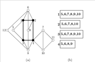
Figure 1: (a) A database graph $G_{i}$ with the current state of FS${}^{\textrm{3}}$’s random walk (b) Neighborhood information of the current state (1,2,3,4)

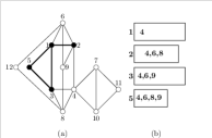
Figure 2: (a) The state of random walk on $G_{i}$ (Figure 2) after one transition (b) Updated Neighborhood information

In FS${}^{\textrm{3}}$, we have used two kinds of scoring functions: $s_{1}$ and $s_{2}$. For a subgraph $g$, $s_{1}(g)$ is the average of the (actual) support of the constituting edges of $g$. Mathematically, $s_{1}(g)=\frac{1}{|E(g)|}\sum_{e\in E(g)}{support(e)}$. $s_{2}(g)$ is the cardinality of the intersection set generated by intersecting the support-set of each of the constituting edges of $g$, i.e., $s_{2}(g)=\left|\bigcap_{e\in E(g)}{support(e)}\right|$. The intuition behind these choices is that if $g$ is frequent, all its edges are frequent, so its score $s_{1}(g)$ is high, same is true for $s_{2}(g)$. The reverse is not necessarily true, i.e., there can be a graph, for which the average support or the set intersection count of its edge-set is high, but the graph is infrequent, so the above scoring functions may sample a few false positive (however, no false negative) patterns. Nevertheless, in real-life graphs the actual support of a subgraph is significantly correlated with its $s_{1}$ and $s_{2}$ score, which we will show in the experiment section. Besides, when the sampling process discovers a $p$-subgraph, its scores can be computed instantly from the support-set of its edges—later can be obtained cheaply during the initial read of the database graphs.

Lemma 1

$s_{1}(g)\geq support(g)$ and $s_{2}(g)\geq support(g)$

Proof:

See appendix.  

State Transition: FS${}^{\textrm{3}}$’s MCMC walk changes state by walking from one $p$-subgraph (say $g$) to a neighboring $p$-subgraph. In our neighborhood definition, for a $p$-subgraph all other $p$-subgraphs that have $p-1$ vertices in common are its neighbor subgraph/state. To obtain a neighbor subgraph of $g$, FS${}^{\textrm{3}}$ simply replaces one of the existing vertices of $g$ with another vertex which is not part of $g$ but is adjacent to one of $g$’s vertices. Also, note that in $g$, if FS${}^{\textrm{3}}$ includes all the edges of $G_{i}$ that are induced by the set of the selected vertices, the sampled subgraph of FS${}^{\textrm{3}}$ is always a connected induced subgraph of the database graphs. On the other hand, if it does not enforce this restriction, the sampled subgraph is a non-induced subgraph. Another important fact is that the neighborhood relation that is defined above is symmetric, which is important in MCMC walk for maintaining the detailed balance equation [23].

Example: Suppose FS${}^{\textrm{3}}$ is sampling $4$-subgraphs from the graph $G_{i}$ shown in Figure 2(a) using MCMC sampling. Let, at any given time the $4$-subgraph $\langle 1,2,3,4\rangle$ (shown in bold lines) is the existing state of this walk. Figure 2(b) lists all the neighbor states of this state. In this figure, the box labeled by $x$ contains all the vertices that can be used as a replacement of vertex $x$ to get a neighbor. For example, one of the neighbor states of the above state is $\langle 1,2,3,5\rangle$, which can be obtained by replacing the vertex $4$ by the vertex $5$. If the FS${}^{\textrm{3}}$’s random walk transition chooses to go to the neighbor state $\langle 1,2,3,5\rangle$, it can do it simply by adding the vertex 5 (a vertex in the box labeled by 4) and deleting the vertex $4$. While adding vertex 5, it adds both the induced edges $(1,5)$ and $(3,5)$ for obtaining an induced subgraph, but adding a random subset of the set of induced edges would have sampled a $p$-subgraph which is not necessarily induced. The updated state of the random walk along with the updated neighbor-list is shown in Figure 2.  

Proposal Distribution: As discussed in Section II-B, for applying MH algorithm, we also need to decide on a proposal distribution, $q$. For FS${}^{\textrm{3}}$’s random walk the proposal distribution is uniform, i.e., in the proposal step FS${}^{\textrm{3}}$ chooses one of $g$’s neighbors uniformly. If a $p$-subgraph $g$ has $d_{g}$ neighbors, and $h$ is one of them, using proposal distribution, the probability of choosing $h$ from $g$ is $q(g,h)=1/d_{g}$.

SampleIndSubGraph($G_{i},p$)
    1$x\mathrel{\hskip 1.0pt=\hskip 1.0pt}$ State saved at $G_{i}$ 2$d_{x}\mathrel{\hskip 1.0pt=\hskip 1.0pt}$ Neighbor-count of $x$ 3$a\_sup_{x}\mathrel{\hskip 1.0pt=\hskip 1.0pt}$ score of graph $x$ 4while (a neighbor state $y$ is not found) 5 $y\mathrel{\hskip 1.0pt=\hskip 1.0pt}$ a random neighbor of $x$ 6 $d_{y}\mathrel{\hskip 1.0pt=\hskip 1.0pt}$ Possible neighbor of $y$ 7 $a\_sup_{y}\mathrel{\hskip 1.0pt=\hskip 1.0pt}$ score of graph $y$ 8 $accp\_val\mathrel{\hskip 1.0pt=\hskip 1.0pt}$ ${(d_{x}*a\_sup_{y})}/{(d_{y}*a\_sup_{x})}$ 9 $accp\_probablility\mathrel{\hskip 1.0pt=\hskip 1.0pt}$ $min(1,accp\_val)$ 10 if $uniform(0,1)\leq accp\_probability$ 11 return $y$

Figure 3: SampleIndSubGraph  Pseudocode

In Figure 3 we show the MH subroutine that samples a $p$-subgraph from a database graph $G_{i}$. In Line 1, it obtains the $p$-subgraph, $x$ (a state of the Markov chain) that was saved during the last sampling from $G_{i}$ in one of the previous iterations. If the saved state is empty (happens only if it is the first graph sampled from $G_{i}$), it simply obtains one of the $p$-subgraphs by growing from a random edge of $G_{i}$ and returns it. In Line 2, it populates the neighbors of $x$ and returns the neighbor-count. In Line 3, it computes the score of the graph $x$ based on the chosen scoring function ($s_{1}$ or $s_{2}$). It then chooses $y$ uniformly from all the neighbors of $x$, populates the neighbors of $y$ and computes $y$’s score (Line 5-7). Considering the chosen scoring function as the desired target distribution, it computes the acceptance probability of the transition from $x$ to $y$ using Equation 1. The while loop (Line 4-11) continues until a valid next state (a neighboring $p$-subgraph) is found. It then returns the newly sampled subgraph $y$.

Lemma 2

FS${}^{\textrm{3}}$’s random walk is ergodic.

Proof:

See appendix.  

Lemma 3

The random walk of FS${}^{\textrm{3}}$ achieves the target probability distribution, which is proportional to the chosen scoring function ($s_{i}$)

Proof:

See appendix.  

IV-B Queue Manager

FS${}^{\textrm{3}}$ runs the $p$-subgraph sampler for a large number of iterations so that in these iterations, the most frequent patterns have a chance to be sampled a number of times that is proportional to its support. Since the number of possible $p$-subgraphs in a database of large graphs can be very large, it may not be feasible to store all of them in the main memory. So FS${}^{\textrm{3}}$ stores only a finite number of best graphs in a priority queue. The queue manager component of FS${}^{\textrm{3}}$ implements the policy of this priority queue (PQ).

For a graph, $g$, stored in the PQ, the queue manager stores four pieces of information regarding the graph: (1) the canonical label  of $g$; (2) the expected-support value ($support_{a}(g)$) at that instance along with the support-list; (3) the score of $g$, i.e. $s_{1}(g)$ or $s_{2}(g)$ depending on which of the target distribution is used; and (4) the time (iteration counter is used as time variable) when the $support_{a}(g)$ was last incremented. The canonical label is used to uniquely identify a graph in PQ to overcome the fact that different sampling iterations may return different isomorphic forms of the same graph. The other pieces of information are used to implement the policy of the PQ.

Queue Eviction Strategy If the new sample is an existing graph in PQ, no eviction is necessary. We simply insert the id of the corresponding database graph (from where the sample was obtained) into the support-list of the graph and update the time variable. In case the id already is present in the support-list, nothing happens. On the other hand, if the new sample is a graph that does not present in PQ and PQ is full, we may choose to accommodate the new graph by evicting one of the graphs in the PQ, if certain conditions are satisfied.

To expedite the eviction decision, we maintain a total order in the PQ using a composite order criterion and the last graph in that total order is possibly evicted. The order uses three variables in lexicographical order: (1) expected-support (high to low); (2) score value, $s_{1}$ or $s_{2}$, depending on which one is used as the target distribution of the MCMC sampling (high to low); and (3) time (recent to old). Thus, the graph with the least expected support occupies the last position in PQ. However, if more than one graphs have the same value for the least expected-support, the tie situation is resolved by placing the graph with the smallest score value in the last position. Note that for FS${}^{\textrm{3}}$’s sampling, tie on expected-count is common as the search space is very large. If there is a tie for the score value also, it is resolved by considering the graph with the oldest update time. The intuition behind the above eviction mechanism is easy to understand; The pattern in the last position has small expected-support (first criterion), or small score, $s_{1}$ or $s_{2}$ (second criterion), or it is not being sampled from different graphs for a long time (third criterion), which makes it less likely to be frequent.

However, FS${}^{\textrm{3}}$’s queue manager does not simply evict the last element in PQ to insert the newly sampled graph (say, $g$), rather it first confirms whether $g$ is a better replacement for the graph that would be evicted from the PQ. The decision is made by using the following heuristic. If the average of the scores ($s_{1}$ or $s_{2}$) of the graphs that are at the tail (lower half) of the PQ is smaller than $s_{1}(g)$ (or $s_{2}(g)$), then $g$ is considered as a better replacement, and the last graph in the sorted order is evicted. If the above condition does not satisfy, graph $g$ is simply ignored, and the sampling continues. The biggest advantage of this conditional eviction is that FS${}^{\textrm{3}}$ does not generate the canonical code of $g$, if $g$ is an unpromising pattern. Since, canonical code generation is much costlier than sampling, the time saved by avoiding the code generation can be spent for performing many other sampling iterations. For implementing the data structure of queue manager with the queue eviction policies, FS${}^{\textrm{3}}$ uses multi-index map data structure , which sorts the graphs uniquely on the canonical label and non-uniquely on the various criteria that we describe above.

FS${}^{\textrm{3}}$$({\cal G},p,mIter)$
     ${\cal G}$: Graph Database, $p$: Size of the subgraph $mIter$: Number of samples 1$iter\mathrel{\hskip 1.0pt=\hskip 1.0pt}0$, $Q\mathrel{\hskip 1.0pt=\hskip 1.0pt}\emptyset$ 2while $iter\leq mIter$ 3 $iter=iter+1$ 4 Select a graph $G\in{\cal G}$ uniformly 5 $h\mathrel{\hskip 1.0pt=\hskip 1.0pt}\textnormal{SampleIndSubgraph}(G,p)$ 6 if $Q.full=true$ and $~{}~{}~{}~{}~{}~{}~{}~{}~{}~{}~{}~{}~{}~{}~{}~{}~{}~{}h.score()<Q.lowerHalfAvgScore()$ 7 continue 8 $h.code\mathrel{\hskip 1.0pt=\hskip 1.0pt}\textnormal{GenCanCode}(h)$ 9 if $h\in Q$ 10 $prevSupport=h.idset.size()$ 11 $h.idset=h.idset\cup G.id$ 12 if $h.idset.size()>prevSupport$ 13 $h.insertTime=iter$ 14 else 15 if $Q.full=true$ 16 $Q.evictLast()$ 17 $h.idset=\{G.id\}$ 18 $h.insertTime=iter$ 19 $Q=Q\cup\{h\}$ 20return $Q$

Figure 4: FS${}^{\textrm{3}}$ Pseudocode

IV-C Theoretical Analysis of FS${}^{\textrm{3}}$

Theoretical analysis of FS${}^{\textrm{3}}$ is difficult as the distribution of $p$-subgraphs is different for different datasets. We perform a theoretical analysis using a uniform distribution which is given in the Appendix.

IV-D FS${}^{\textrm{3}}$ Pseudocode

The entire pseudo-code of FS${}^{\textrm{3}}$ is shown in Figure 4. It samples a $p$-subgraph ($h$) from a randomly selected database graph $G$ by calling SampleIndSubGraph routine. Line 7 ensures that the sampled graph $h$ is ignored (and its canonical code is not generated) if its score is not better than the average score of the lower-half graphs in the PQ. In subsequent lines, If $h$ does not present in the priority queue PQ, FS${}^{\textrm{3}}$ saves the graph $h$ in the priority queue along with its support-list which contains only $G.id$. On the other hand, if $h$ exists in the queue, FS${}^{\textrm{3}}$ updates its support list, and also updates its insert-time variable. For each graph $G\in{\cal G}$, the sampling process saves the latest visiting graph (state), so that any later sampling from this graph starts from the saved state. From this perspective, FS${}^{\textrm{3}}$ runs $|{\cal G}|$ copy of MCMC samplers, one for one of the input graphs in ${\cal G}$.

V Experiments

We implement FS${}^{\textrm{3}}$ as a C++ program, and perform a set of experiments for evaluating its performance for mining frequent subgraphs of a given size. We run all the experiments in a computer with 2.60GHz processor and 4GB RAM running Linux operating system.

V-A Datasets

We use three datasets for our experiments. The first is a protein structure dataset that we call PS. In this dataset, each graph represents the structure of a protein in the TIM (Triose Phosphate Isomerage) family. To construct a graph from a protein structure, we treat each amino acid residue as a vertex (labeled by letter code of the amino acids), and connect two vertices with an edge if the Euclidean distance between the $C_{\alpha}$ atom of the corresponding residues is at most $8$Å. An edge also has a label of 1 or 2 based on whether the distance is below or above $4$Å. Frequent subgraphs in such a dataset are common structure of the homologous proteins. The statistics of this dataset are available in Table I; the same table also shows that existing graph mining methods are not able to mine subgraphs from this dataset. Our second dataset is a synthetic dataset (we call it Syn) that we build using the generator used in [24] with parameters (ngraphs, size, nnodel, nedgel) $=$(0.1, 250, 20, 5). The subgraph space of this dataset is even larger than the PS dataset, and hence, it is more difficult to mine. Our last dataset is called Mutagenicity II (we will call it Mutagen dataset for abbreviation); it has been used in earlier works on graph mining [25]. Note that, it contains mostly chemical graph (avg. vertex count=14, avg. edge count=14), and existing graph mining methods can mine this dataset easily. We use this dataset only for comparing precision because ground truth of frequent subgraphs for this graph is easy to obtain.

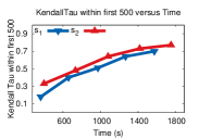
(a) #$p=7$

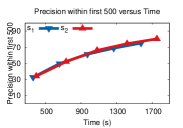
(b) #$p=7$

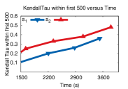
(c) #$p=8$

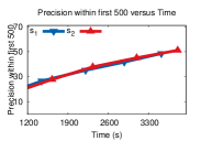
(d) #$p=8$

Figure 5: Kendall Tau, Precsion within first 500 for PS Dataset

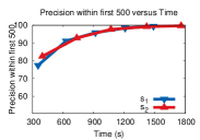
(a) $p=6$

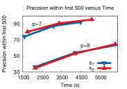
(b) $p=7,8$

Figure 6: Effect of increasing running time for FS${}^{\textrm{3}}$versus precision for PS Dataset

V-B Experiment Setup

FS${}^{\textrm{3}}$ finds top-$k$ frequent subgraphs with high probability. So, we measure the performance of FS${}^{\textrm{3}}$ both from the execution time, and the quality of results. To obtain the quality, we use two metrics, that are pr@500 (precision at 500), and rank correlation metric, Tau-$b$. If ${\cal H}_{a}$ is the set of 500 most frequent subgraphs of a given size obtained by FS${}^{\textrm{3}}$  and ${\cal H}$ is the corresponding true set of the same size based on actual support, the metric pr@500 is $\frac{\left|{\cal H}\cup{\cal H}_{a}\right|\times 100}{500}$; i.e, it finds the percentage of graphs in ${\cal H}$ that are also presented in ${\cal H}_{a}$. The higher the value of pr@500, the better the performance of FS${}^{\textrm{3}}$. Note that, for a graph dataset that has one billion of subgraphs of a given size, sampling frequent graphs that belong to set ${\cal H}$ is not easy. A dumb sampler has a pr@500 value equal to 500 divided by one billion.

The metric, pr@500 only considers the presence or absence of a true positive (actually frequent) graph in ${\cal H}_{a}$, but it does not consider the order of graphs in ${\cal H}_{a}$ and the order of graphs in ${\cal H}$; in other words, it does not check whether actual support and expected support (as obtained by FS${}^{\textrm{3}}$) have positive correlation or not. For this we use Tau-$b$ metric, which is the rank correlation between actual support and expected support of the objects in ${\cal H}\cup{\cal H}_{a}$. Tau-$b$ varies between -1 and 1. A value of 0 means no correlation, and the higher the value above 0, the better the correlation. A strong correlation provides the evidence that FS${}^{\textrm{3}}$ can indeed rank the patterns in the order of their actual support.

For computing pr@500 and Tau-$b$, we need to know the true set of top 500 frequent patterns of a given size. This is difficult to obtain for PS and Syn dataset, which we cannot mine with the existing methods. To solve this problem, we have used GTrieScanner [26]; for an input graph GTrieScanner dumps all of its $p$-subgraphs; by running this program for all the input graphs in a graph database, and grouping those by the canonical-code of those $p$-subgraphs, we compute the actual support value of all the $p$-subgraphs. Such exhaustive enumeration of actual support was only possible for the Mutagen dataset for all sizes, and for the PS and Syn datasets for size up to 8. For the later two datasets, for size larger than 8, the size of the dump of GTrieScanner exceeds more than 1 TB of physical space of a hard-disk, which is impossible for us to post-process. Also note that, GTrieScanner generates only the induced subgraphs, so for this comparison we run FS${}^{\textrm{3}}$ for its induced subgraph sampling setup.

Performance of FS${}^{\textrm{3}}$ depends on the number of iterations, scoring function used, size of the sampled patterns, and of-course the dataset. Also, choices of these values affect the running time of an iteration. So, when comparing among different sampling scenarios of FS${}^{\textrm{3}}$  we plot the performance metric along the $y$-axis and the time along the $x$ axis, and use a smooth curve to show the trend. Since, our method is randomized, all performance metric values are average of 10 distinct runs. We keep the priority queue size at 100K for all our experiments, unless specified otherwise (memory footprint around 200 MB). Majority of our results are obtained by running experiments on the PS dataset.

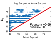
(a) Correlation with $s_{1}$

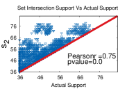
(b) Correlation with $s_{2}$

Figure 7: Correlation between support and score of a pattern

V-C Correlation between actual support and scores

In Figure 7(a) and 7(b), we show the scatter plot between actual support vs $s_{1}$ value (left plot) and $s_{2}$ value (right plot) of these patterns. This significant correlation between actual support and scores enables the FS${}^{\textrm{3}}$’s MCMC walk to be able to sample top-$k$ frequent patterns effectively.

V-D Performance of FS${}^{\textrm{3}}$ for different sampling setups

In this experiment, we compare the performance of FS${}^{\textrm{3}}$ using the scoring function $s_{1}$ and $s_{2}$ on PS dataset for size 7 and 8 (the true set (${\cal H}$) is known for these sizes). Figure 5 shows the results; in the left, we show the results (pr@500, and Tau-$b$ vs time) for size 7, and in the right for the size 8. ¿From the figure, we see that for both the scores, with increasing number of samples both pr@500, and Tau-$b$ metrics increase almost linearly. Another observation from this figure is that the choice of score ($s_{1}$ or $s_{2}$) has small effect on the performance metric, specifically for pr@500. For Tau-$b$, score $s_{2}$ performs slightly better than the score $s_{1}$. This trend holds for other two datasets also.

Now, we comment on the values of pr@500 and Tau-$b$ on these figures. ¿From Figure 5(d), we see that for size 8, 1500 seconds of running of FS${}^{\textrm{3}}$ yields pr@500 value of 28%, which increases to 50% for 3700 seconds, i.e., within an hour of sampling time, FS${}^{\textrm{3}}$ finds 50% of the most frequent graphs from a sampling space of 0.95 billions graphs (See Table I). Also note that the fastest graph mining algorithm, Gaston, could not mine this dataset in 16 hours of time, for 11% support and the max-size of 8. Also, within an hour of running, FS${}^{\textrm{3}}$’s Tau-$b$ value reaches up to 0.42, which is a significant correlation. Now, for size 7, the performance is understandably better than the size 8 (see figure 5(a) and (b)), because its search space contains smaller number of subgraphs—157 millions as reported in Table I.

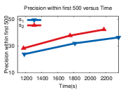
(a) Syn, #p = 6

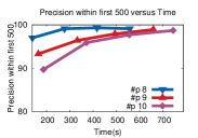
(b) Mutagen, #p = 8, 9, 10

Figure 8: Precision for Synthetic and Mutagen Dataset

What happens if we run FS${}^{\textrm{3}}$ for even more iterations? The performance keeps improving as we see in Figure 6. By running the sampler for 20 minutes for size 6, 1.4 hour for size 7, and 1.8 hour for size 8, we obtain 99%, 95% and 65% value for the pr@500. The linear trend of the curve for size 8 shows that by running more time, the pr@500 can be improved even further.

We also run the above set of experiments for the other two datasets. In Figure 8(a), we show the results for Syn dataset for size 6, for which we obtain pr@500 value of 42% in around 35 minutes. The performance on this dataset is poorer than the PS dataset, because search space in this dataset is much larger than the PS dataset. We cannot show results for higher size for this dataset as we could not generate the ground truth. In Figure 8(b), we show the results for the Mutagen dataset, which has the smallest subgraph space, so for sizes 8, 9, and 10 this dataset achieves more than 90% pr@500 within 10 minutes.

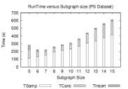
(a) PS

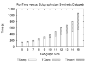
(b) Syn

Figure 9: Runtime performance of FS${}^{\textrm{3}}$ for sampling subgraphs of different sizes

V-E FS${}^{\textrm{3}}$’s scalability with the size, $p$

The execution time of FS${}^{\textrm{3}}$ has three components: sampling time, canonical code generation time, and queue insertion time. In this experiment, we check how these times vary as we vary the desired size of the subgraphs to be sampled ($p$ value). For this, we use PS and Syn datasets, and use $s_{2}$ scoring function. Figure 9 shows the results. As we see in the plots, the execution time increases almost linearly with the value of $p$ for both the datasets. Also, FS${}^{\textrm{3}}$ spends the majority of its execution time for sampling as it does not generate canonical code in many of its iterations. Queue insertion time is negligible compared to sampling and canonical code generation time.

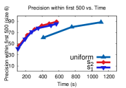
(a) Effect of Target Distribution

Queue	Precision	Kendal	Time
Size			(s)
(m)
0.5	52.3	35.4	3997
1.0	54.2	42.4	4211
2.0	53.9	55.4	4645

(b) Effect of Queue Size

Figure 10: Effect of Queue Size and Target Distribution

V-F Impact of target distribution and queue size

FS${}^{\textrm{3}}$’s MCMC sampling uses $s_{1}$ or $s_{2}$ score to construct its target distribution. In this experiment, we validate the impact of these choices by comparing their performances with a case, where the target distribution is uniform, i.e., each of the $p$-subgraphs of a database graph $G_{i}$ has equal likelihood to be visited, that is the score of any $p$-subgraph is 1, a constant (let’s call it uniform-FS${}^{\textrm{3}}$). For comparison, we use the pr@500 metric. Figure 10(a) shows the result for PS dataset for size 6. It is clear from this figure that by adopting $s_{1}(g)$ or $s_{2}(g)$ as the target distribution, we achieve higher pr@500 at a faster rate. For example, within 7 minutes of sampling, the pr@500 score of uniform-FS${}^{\textrm{3}}$ is around 55%; on the other hand, for the same time, the pr@500 score is around 85% for both $s_{1}(G)$ and $s_{2}(G)$.

For all our experiments we kept the priority queue size fixed to 100K. If we increase the queue size, the memory footprint of the algorithm will increase, but the method will be more accurate, as it will be able to store a large number of potential frequent graphs that may turn out to be frequent at a later time. The improvement is more prominent for the Tau-$b$ metric than the pr@500 metric as shown in Figure 10(b) for PS dataset and subgraph size 8.

V-G Impact of k on FS${}^{\textrm{3}}$

We also study the performance of FS${}^{\textrm{3}}$ for different choices of $k$ value. For this experiment, we use PS dataset, $p$=7. Figure 11 shows the corresponding result. In Figure 11(a), we plot the Pr@k values and in Figure 11(b), we plot the Kendall Tau values for different $k$’s between $100$ and $500$. We calculate both the statistics by taking the average of $10$ independent runs. As we can see, for the entire range of $k$ values, the performance remains almost constant.

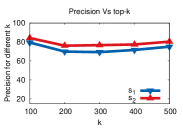
(a) Precision

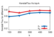
(b) Kendall Tau

Figure 11: Performance of FS${}^{\textrm{3}}$ for different $k$

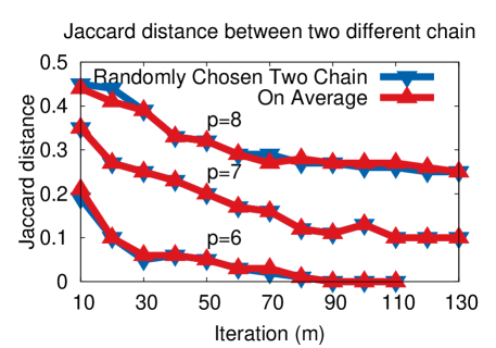
Figure 12: Jaccard Distance vs Iteration

V-H Choosing iteration counts

We design a more sophisticated stopping criteria using Gelman-Rubin Diagnostics [27]. Figure 12 shows the relation between Jaccard distance and iteration count for the number of chain $10$. As we can see, for increasingly larger iteration count, the Jaccard distance among the top-$k$ patterns from different chains diminishes and for sufficiently large value, it converges to a small value.

VI Conclusion

In this paper, we present FS${}^{\textrm{3}}$, a sampling based method for finding frequent induced subgraph of a given size. For large input graphs, existing algorithms for frequent subgraph mining are completely infeasible; whereas FS${}^{\textrm{3}}$ can return a small set of probabilistically frequent patterns of desired size within a small amount of time. Our experiments show that the expected support of the graphs that FS${}^{\textrm{3}}$ samples has excellent rank correlation with their actual support. The theoretical proof relevant in this paper has been presented in the appendix section.

Lemma 1

$s_{1}(g)\geq support(g)$ and $s_{2}(g)\geq support(g)$

Proof:

Consider an edge $e\in E(g)$. Since $e\in E(g)$, $support\mbox{-}set(e)\supseteq support\mbox{-}set(g)$, hence $support(e)\geq support(g)$. Since this hold for all the edges, average-support of the edges is an upper bound of the support of $g$; hence, $s_{1}(g)\geq support(g)$.

To compute $s_{2}(g)$ we intersect the $support\mbox{-}set(e)$ of all edges $e\in g$. Thus, $s_{2}(g)$ considers the support of the edge-set of $g$, without considering the graphical constraint imposed by $g$, so $s_{2}(g)\geq support(g)$.  

Lemma 2

FS${}^{\textrm{3}}$’s random walk is ergodic.

Proof:

A Markov chain is ergodic if it converges to a stationary distribution. To obtain a stationary distribution the random walk needs to be finite, irreducible and aperiodic. The state space consisting of all $p$-subgraphs is finite for a given $p$. We also assume that the input graph $G$ is connected, so in this random walk any state $y$ is reachable from any state $x$ with a positive probability and vice versa, so the random walk is irreducible. Finally, the walk can be made aperiodic by allocating a self-loop probability at every node. Thus the lemma is proved.  

Lemma 3

The random walk of FS${}^{\textrm{3}}$ achieves the target probability distribution, which is proportional to the chosen scoring function ($s_{i}$)

Proof:

An ergodic random walk achieves the target probability distribution if it satisfies the reversibility condition i.e., for two neighboring states $x$ and $y$, $\pi(x)T(x,y)=\pi(y)T(y,x)$, where $\pi$ is the target distribution and $T(x,y)$ is the transition probability from $x$ to $y$. For FS${}^{\textrm{3}}$ the target distribution for a graph $x$, $\pi(x)=\frac{s_{i}(x)}{K}$, where $K$ is a normalizing constant. Now, from Figure 3, it is easy to see that $\pi(x)T(x,y)=\frac{s_{i}(x)}{K\cdot d_{x}}\min\left\{1,\frac{d_{x}*s_{i}(y)}{d_{y}*s_{i}(x)}\right\}=\frac{1}{K}\min\left\{\frac{s_{i}(x)}{d_{x}},\frac{s_{i}(y)}{d_{y}}\right\}$. Since the neighborhood relation is symmetric, there can be a transition from the state $y$ to $x$ and using that we have $\pi(y)T(y,x)=\frac{s_{i}(y)}{K\cdot d_{y}}\min\left\{1,\frac{d_{y}*s_{i}(x)}{d_{x}*s_{i}(y)}\right\}=\frac{1}{K}\min\left\{\frac{s_{i}(y)}{d_{y}},\frac{s_{i}(x)}{d_{x}}\right\}$. So, $\pi(x)T(x,y)=\pi(y)T(y,x)$, which proves the lemma. 

Theoretical Analysis of FS${}^{\textrm{3}}$ FS${}^{\textrm{3}}$ ranks the subgraph patterns based on the expected support ($support_{a}$). In this section, we analyze the expected value of $support_{a}$ for a $p$-subgraph pattern $g$. To simplify the analysis, we will assume that in each sampling iteration (in Line 5 of Figure 4), FS${}^{\textrm{3}}$ returns one of the $p$-subgraphs of the chosen database graph uniformly. This assumption actually perform a worst-case analysis, because in general FS${}^{\textrm{3}}$ performs a biased sampling in which the presumable frequent $p$-subgraphs are sampled with higher probability.

Let, ${\cal G}=\{G_{1},G_{2},\ldots,G_{n}\}$ be a graph database with $n$ graphs. Let’s use $x_{j}$ to denote the number of distinct $p$-subgraphs in the graph $G_{j}$. Assume that the (induced) support of a subgraph pattern $g$ in the database ${\cal G}$ is $s$, and the id of the graphs in which $g$ occurs are $z_{1},z_{2},\cdots,z_{s}$.

If FS${}^{\textrm{3}}$ makes $t$ sampling iterations, on average $t/n$ samples are obtained from the graph $G_{z_{i}:1\leq i\leq s}$. Under the uniform sampling assumption, the probability of sampling $g$ from $G_{z_{i}}$ in at least one of $t/n$ iterations is equal to $1-\left(1-1/x_{z_{i}}\right)^{t/n}$. Since the number of sampling iterations is typically very large, the above term is equal to $1-(1-\frac{t}{n\cdot x_{z_{i}}})=\frac{t}{n\cdot x_{z_{i}}}$. So, the expected support of $g$, $E\big{[}support_{a}(g)\big{]}=\frac{t}{n}\times(1/x_{z_{1}}+1/x_{z_{2}}+\cdots+1/x_{z_{s}})$. If the number of samples are in the same order as the number of $p$-subgraphs in the database graphs, the expected support converges to the actual support and the estimation is unbiased. Note that, even if the value of $x_{z_{i}}$ are large (in the order of millions), FS${}^{\textrm{3}}$ can sample millions of iterations in a few minutes, thus it can bring the $support_{a}$ value close to the actual support effectively. On the other hand, existing methods are not scalable as performing millions of SI test will take months, if not years.

However, FS${}^{\textrm{3}}$ performs much better than a uniform sampler, as it actually performs a support-biased sampling. In real-life datasets, the support of $p$-subgraphs follows a heavy-tail distribution, in which a small number of truly frequent patterns have high support, but the majority of the $p$-subgraphs have small support. Thus, the success probability of sampling a frequent pattern $g$ from the graph $G_{z_{i}}$ is much higher than $\frac{t}{n\cdot x_{z_{i}}}$. In Section V-F, we will compare between FS${}^{\textrm{3}}$ and a modified version of FS${}^{\textrm{3}}$ that uses the uniform sampling to show that FS${}^{\textrm{3}}$’s performance is substantially better.

References

- [1] M. Deshpande, M. Kuramochi, N. Wale, and G. Karypis, “Frequent substructure-based approaches for classifying chemical compounds,” IEEE Trans. on Knowl. and Data Eng., vol. 17, no. 8, pp. 1036–1050, 2005.
- [2] H. Hu, X. Yan, Y. Huang, J. Han, and X. J. Zhou, “Mining coherent dense subgraphs across massive biological networks for functional discovery,” Bioinformatics, vol. 21, 2005.
- [3] N. Jin, C. Young, and W. Wang, “Gaia: graph classification using evolutionary computation,” in Proceedings of SIGMOD. ACM, 2010, pp. 879–890.
- [4] X. Yan, P. S. Yu, and J. Han, “Graph indexing: a frequent structure-based approach,” in Proc. of SIGMOD, 2004, pp. 335–346.
- [5] V. Chaoji, M. Hasan, S. Salem, J. Besson, and M. Zaki, “ORIGAMI: A Novel and Effective Approach for Mining Representative Orthogonal Graph Patterns,” Statistical Analysis and Data Mining, vol. 1, no. 2, pp. 67–84, June 2008.
- [6] A. Inokuchi, T. Washio, and H. Motoda, “An apriori-based algorithm for mining frequent substructures from graph data,” in Proc. of PKDD, 2000, pp. 13–23.
- [7] M. Kuramochi and G. Karypis, “An Efficient Algorithm for Discovering Frequent Subgraphs,” IEEE Trans. on Knowledge and Data Engineering, vol. 16, no. 9, pp. 1038–1051, 2004.
- [8] X. Yan and J. Han, “gspan: Graph-based substructure pattern mining,” in Proc. of ICDM, 2002, pp. 721–724.
- [9] S. Nijssen and J. N. Kok, “The gaston tool for frequent subgraph mining,” Electr. Notes Theor. Comput. Sci., vol. 127, no. 1, pp. 77–87, 2005.
- [10] M. Al Hasan and M. J. Zaki, “Output space sampling for graph patterns,” Proc. VLDB Endow., vol. 2, no. 1, pp. 730–741, 2009.
- [11] M. Wörlein, T. Meinl, I. Fischer, and M. Philippsen, “A quantitative comparison of the subgraph miners mofa, gspan, ffsm, and gaston,” in Proc. of PKDD, 2005, pp. 392–403.
- [12] X. Yan, H. Cheng, J. Han, and P. S. Yu, “Mining significant graph patterns by leap search,” in Proc. of SIGMOD, 2008, pp. 433–444.
- [13] M.Thoma, H. Cheng, A. Gretton, J. Han, H. Kriegel, A. Smola, L. Song, P. Yu, X. Yan, and K. Borgwardt, “Near-optimal supervised feature selection among frequent subgraphs,” in Proc. of SDM, 2009, pp. 1076–1987.
- [14] M. A. Hasan and M. Zaki, “Musk: Uniform sampling of maximal patterns,” in In Proc. of Ninth SIAM Data Mining, 2009, pp. 650–661.
- [15] A. Inokuchi, T. Washio, K. Nishimura, and H. Motoda, “A fast algorithm for mining frequent connected subgraphs,” IBM Research, Tech. Rep., 2002.
- [16] J. Huan, W. W. 0010, J. Prins, and J. Yang, “SPIN: mining maximal frequent subgraphs from graph databases,” in KDD. ACM, 2004, pp. 581–586.
- [17] L. Thomas, S. Valluri, and K. Karlapalem, “Margin: Maximal frequent subgraph mining,” in Data Mining, 2006. ICDM ’06. Sixth International Conference on, 2006, pp. 1097–1101.
- [18] X. Yan and J. Han, “Closegraph: mining closed frequent graph patterns,” in Proceedings of the ninth ACM SIGKDD international conference on Knowledge discovery and data mining. New York, NY, USA: ACM, 2003, pp. 286–295.
- [19] T. Horváth, J. Ramon, and S. Wrobel, “Frequent subgraph mining in outerplanar graphs,” in Proceedings of SIGKDD, 2006, pp. 197–206.
- [20] T. Horváth and J. Ramon, “Efficient frequent connected subgraph mining in graphs of bounded tree-width,” Theor. Comput. Sci., vol. 411, no. 31-33, pp. 2784–2797, Jun. 2010.
- [21] R. Vijayalakshmi, R. Nadarajan, J. F. Roddick, M. Thilaga, and P. Nirmala, “Fp-graphminer-a fast frequent pattern mining algorithm for network graphs,” Journal of Graph Algorithms and Applications, vol. 15, no. 6, pp. 753–776, 2011.
- [22] E. Keogh, S. Lonardi, and C. A. Ratanamahatana, “Towards parameter-free data mining,” in Proc. of SIGKDD, 2004, pp. 206–215.
- [23] R. R. Y. and K. D. K., Simulation and the Monte Carlo Method. John Wiley and Sons, 2008.
- [24] J. Cheng, Y. Ke, W. Ng, and A. Lu, “Fg-index: towards verification-free query processing on graph databases,” in Proc. of SIGMOD, 2007, pp. 857–872.
- [25] B. Bringmann, A. Zimmermann, L. D. Raedt, and S. Nijssen, “Don’t be afraid of simpler patterns,” in PKDD 2006, 2006, pp. 55–66.
- [26] P. Ribeiro and F. Silva, “G-tries: an efficient data structure for discovering network motifs,” in Proc. ACM Symp. on Applied Computing, 2010, pp. 1559–1566.
- [27] A. Gelman and D. B. Rubin, “Inference from iterative simulation using multiple sequences,” Stat. Sci., vol. 7, pp. 457–472, 1992.