Characterizing and Subsetting Big Data Workloads

Abstract

Big data benchmark suites must include a diversity of data and workloads to be useful in fairly evaluating big data systems and architectures. However, using truly comprehensive benchmarks poses great challenges for the architecture community. First, we need to thoroughly understand the behaviors of a variety of workloads. Second, our usual simulation-based research methods become prohibitively expensive for big data. As big data is an emerging field, more and more software stacks are being proposed to facilitate the development of big data applications, which aggravates these challenges.

In this paper, we first use Principle Component Analysis (PCA) to identify the most important characteristics from 45 metrics to characterize big data workloads from BigDataBench, a comprehensive big data benchmark suite. Second, we apply a clustering technique to the principle components obtained from the PCA to investigate the similarity among big data workloads, and we verify the importance of including different software stacks for big data benchmarking. Third, we select seven representative big data workloads by removing redundant ones and release the BigDataBench simulation version, which is publicly available from http://prof.ict.ac.cn/BigDataBench/simulatorversion/.

I Introduction

Today, huge amounts of data are being collected in many areas, creating new opportunities to understand phenomena in meteorology, health, finance, and many other sectors. Every two days we create as much information as we did from the dawn of civilization up until 2003, and the pace is increasing [1]. Reports from IDC forecast that from 2005 to 2020, the digital universe will grow by a factor of 300, from 130 exabytes to 40,000 exabytes (i.e., 40 trillion gigabytes) [2]. Turning such big data into valuable information requires the support of big data systems, and the design of such systems is a growing research topic in both academia and industry. In this context, the pressure to develop innovative theories and technologies to improve the performance, energy-efficiency, and cost-effectiveness of big systems rises.

The cornerstone of such research are big data benchmarks that facilitate accurate evaluation of big data systems and a better understanding of the behaviors of big data workloads (applications). Fair evaluation requires diversity in both the data sets and the workloads used in benchmarking big data systems and architectures. Generating such comprehensive and representative benchmarks raises two great challenges for the architecture community. First, the plethora of microarchitectural metrics that can be tracked creates a potentially huge amount of characterization data that can be hard to analyze. Second, the simulation-based approaches that are widely used in architecture research are very time-consuming: simulating complete workloads amounts to an impossible mission. How to address these challenges remains an open question.

More and more software stacks are being proposed to facilitate the development of big data applications. Previous work [3] [4] has shown that software stacks can cause big data workloads to have different user-observed performance. For instance, compared to Hadoop, Spark improves runtime performance by factors of up to 100. Different software stacks should thus be included in the benchmarks, but that aggravates the above challenges by multiplying the number of workloads.

To date, the major efforts on big data benchmarking either propose a comprehensive but a large amount of workloads or only select a few workloads according to so-called popularity [5]. And hence, achieving benchmark comprehensiveness while enabling efficient experimentation is particularly acute in big data systems research. Although many workload subsetting approaches have been proposed [6, 7, 8, 9], these are designed for workloads having significantly different characteristics from big data applications.

In this paper, we propose a general approach to 1) identify the most important metrics for characterizing big data workloads and 2) cull redundant workloads. To demonstrate the effectiveness of the approach, we select two prevalent big data processing software stacks (Hadoop [10] and Spark [3]), single out 32 workloads from BigDataBench [11] to run on these stacks, and evaluate them via 45 typical microarchitectural metrics that represent basic characteristics of modern processors. After applying Principle Component Analysis (PCA) and hierarchical clustering, we find the following:

Software stacks have significant impact on the microarchitectural behaviors of big data workloads. This finding is based on the five observations in Section V-A. We observe that workloads implementing different algorithms running on the same software stack are more likely to have similar behaviors than same-algorithm workloads running on different software stacks (in the first clustering iteration, 80% of clusters consist of workloads that are based on the same software stack). This indicates that (in our experimental setting, at least) the impact of software stacks is greater than that of algorithms. Hence, it is reasonable to say that different software stacks must be included in performing representative and credible evaluations of big data systems. Compared to traditional software stacks, big data software stacks usually have more complex structures. Such designs enable programmers to write less code to achieve their intended goals. The upshot is that the ratio of system software and middleware instructions executed compared to user applications instructions tends to be large, which makes their impact on system behavior large, as well.

We can identify the most important microarchitectural-level metrics for studying the impact of different software stacks. We apply PCA to 45 microarchitectural metrics, finding that the L3 cache miss rate, instruction fetch stalls, data TLB behaviors, and snoop responses are the most important metrics in differentiating Hadoop-based and Spark-based workloads.

We can successfully subset big data workloads. Based on our derived principle components, we employ another clustering technique to select seven representative workloads (out of the original 32) by retaining those exhibiting unique behaviors. We also use a statistical method (Bayesian Information Criterion) to ensure that the clustering is a “good fit” to our workloads. We deploy the representative workloads on a full-system simulator and release the BigDataBench simulator version, which is publicly available from http://prof.ict.ac.cn/BigDataBench/simulatorversion/.

II Background

Measuring big data systems and architectures quantitatively is the foundation of innovative big data research, and a good benchmark suite can make this task much more efficient. When constructing such benchmarks, making their behavior representative of real workloads is important to their success [12, 13]. We choose BigDataBench [11], a recent benchmark suite, for our workload characterization for the following reasons:

1. It covers representative application domains. BigDataBench includes microbenchmarks and applications from search engines, social networks, and e-commerce — i.e., the most important internet services from typical big data application domains.

2. It covers representative workloads. As in the widely used TPC-C benchmark[14], units of computation that appear frequently in the benchmarked application domain are used in benchmark construction.

3. It covers diverse software stacks [15]. In BigDataBench, the offline analytics workloads use Hadoop and Spark, and the interactive analytics and OLAP workloads use Shark, Hive, and etc.

4. It considers data volume and veracity. BigDataBench develops Big Data Generator Suite (BDGS), an open source tool to generate synthetic big data based on six raw data sets [16].

III Methodology

We use the following methodology to analyze the software stack’s impact on big data workloads from a microarchitectural perspective. First we select representative workloads in big data fields. Then we identify a set of microarchitectural metrics that can directly or indirectly reflect program behavior. Finally, we use standard statistical methods in our characterizations.

III-A Workload Selection

We select BigDataBench workloads that include structured, semi-structured, and unstructured data. To minimize the impact of non-workload factors, we ensure the following properties in our comparisons.

Identical Algorithms. All applications we select have two implementations of the same algorithm — a Hadoop-based implementation and a Spark-based implementation. Table I lists the algorithms we use. Recall that the offline analytics workloads contain algorithms implemented directly on Hadoop or Spark, and the interactive analytics workloads involve SQL-like operations on Hive [17] or Shark [18]. Hive operations are interpreted in Hadoop jobs, and Shark operations are interpreted in Spark jobs. Table I lists the workloads we use in this paper.

Identical Data Sets. We use the same data set to drive both the Hadoop-based and Spark-based workloads, i.e., both data formats and data sizes are identical. Table I lists these data sets and formats. The input data size for each workload is determined by the Spark-based implementation, since Spark is an in-memory computing engine. Both the input and intermediate data should fit in memory to attain reasonable experiment time. For each Spark-based workload, we test several input data sets, ranging from several gigabytes to more than 100 gigabytes.

Same Infrastructure. Both workload implementations run on the same cluster under the same software environment (i.e., with the same numbers of threads, the same OS version, and the same JVM version). Section IV gives configuration details.

TABLE I: Representative Data Analysis Workloads

Category	Workload	Problem Size	Data Type	Software Stack
	Sort	80 GB	unstructured sequence file
	WordCount	98 GB	unstructured text
Offline Analytics	Grep	98 GB	unstructured text	Hadoop & Spark
	Naive Bayes	84 GB	semi-structured text
	K-means	44 GB	unstructured text
	PageRank	$2^{24}$ vertices	unstructured graph
	Projection	420 million records
	Filter	420 million records
	Order By	420 million records
Interactive Analytics	Cross product	100 million records		Hive & Shark
	Union	420 million records	structured table
	Difference	100 million records	(e-commerce transaction data set)
	Aggregation	420 million records
	JoinQuery	100 million records
	AggQuery	420 million records
	SelectQuery	420 million records

III-B Microarchitectural Metric Selection

Good workload characterization incorporates a variety of metrics to better gain a comprehensive understanding of the target programs [8]. To analyze microarchitectural behaviors, we choose a broad set of metrics of different types that cover all major characters. We particularly focus on factors that may affect data movement or calculation. For example, a cache miss may delay data movement, and a branch misprediction flushes the pipeline. Table II summarizes them, and we categorize them below.

Instruction Mix. The instruction mix can reflect a workload’s logic and affect performance. Here we consider both the instruction type and the execution mode (i.e., user mode running in ring three and kernel mode running in ring zero).

Cache Behavior. The processor in our experiments has private L1 and L2 caches per core, and all cores share an L3. The L1 cache is split for instructions and data. The L2 and L3 are unified. We track the cache misses per kilo instructions and cache hits per kilo instructions except L1 data cache, noting that for the L1D miss penalties may be hidden by out-of-order cores [19].

Translation Look-aside Buffer (TLB) Behavior. Our processor has a two-level TLB. The first level has separate instruction and data TLBs. The second level is shared. We collect statistics at both levels.

Branch Execution. We consider the miss prediction ratio and the ratio of branch instructions executed to those retired. These reflect how many branch instructions are predicted wrong and how many are flushed.

Pipeline Behavior. Stalls can happen in any part of the pipeline, but superscalar out-of-order processors prevent us from precisely breaking down the execution time [5, 20, 21]. Retirement-centric analysis also has difficulty accounting for how the CPU cycles are used because the pipeline continues executing instructions even when retirement is blocked [22]. Here we focus on counting cycles stalled due to resource conflicts, e.g., reorder buffer full stalls that prevent new instructions from entering the pipeline.

Offcore Requests and Snoop Responses. Offcore requests tell us about individual core requests to the LLC (Last Level Cache). Requests can be classified into data requests, code requests, data write-back requests, and request for ownership (RFO) requests. Snoop responses give us information on the workings of the cache coherence protocol.

Parallelism. We consider Instruction Level Parallelism (ILP) and Memory Level Parallelism (MLP). ILP reflects how many instructions can be executed in one cycle (i.e., the IPC), and MLP reflects how many outstanding cache requests are being processed concurrently.

Operation Intensity. The ratio of computation to memory accesses reflects a workload’s computation pattern. For instance, most big data workloads have a low ratio of floating point operations to memory accesses, whereas HPC workloads generally have high floating point operations to memory accesses ratios [11].

TABLE II: microarchitecture Level Metrics.

Category	No.	Metric Name	Description
Instruction	1	LOAD	load operations’ percentage
Mix	2	STORE	store operations’ percentage
	3	BRANCH	branch operations’ percentage
	4	INTEGER	integer operations’ percentage
	5	FP	X87 floating point operations’ percentage
	6	SSE FP	SSE floating point operations’ percentage
	7	KERNEL MODE	the ratio of instruction running on kernel mode
	8	USER MODE	the ratio of instruction running on user mode
	9	UOPS TO INS	the ratio of micro operation to instruction
Cache Behavior	10	L1I MISS	L1 instruction cache misses per K instructions
	11	L1I HIT	L1 instruction cache hits per K instructions
	12	L2 MISS	L2 cache misses per K instructions
	13	L2 HIT	L2 cache hits per K instructions
	14	L3 MISS	L3 cache misses per K instructions
	15	L3 HIT	L3 cache hits per K instructions
	16	LOAD HIT LFB	loads miss the L1D and hit line fill buffer per K instructions
	17	LOAD HIT L2	loads hit L2 cache per K instructions
	18	LOAD HIT SIBE	loads hit sibling core’s L2 cache per K instructions
	19	LOAD HIT L3	loads hit unshared lines in L3 cache per K instructions
	20	LOAD LLC MISS	loads miss the L3 cache per K instructions
TLB Behavior	21	ITLB MISS	misses in all levels of the instruction TLB per K instructions
	22	ITLB CYCLE	the ratio of instruction TLB miss page walk cycles to total cycles
	23	DTLB MISS	misses in all levels of the data TLB per K instructions
	24	DTLB CYCLE	data TLB miss page walk cycles to total cycles
	25	DATA HIT STLB	DTLB first level misses that hit in the second level TLB per K instructions
Branch	26	BR MISS	branch miss prediction ratio
Execution	27	BR EXE TO RE	the ratio of executed branch instruction to retired branch execution
Pipeline Behavior	28	FETCH STALL	the ratio of instruction fetch stalled cycle to total cycles
	29	ILD STALL	the ratio of Instruction Length Decoder stalled cycle to total cycles
	30	DECODER STALL	the ratio of Decoder stalled cycles to total cycles
	31	RAT STALL	the ratio of Register Allocation Table stalled cycles to total cycles
	32	RESOURCE STALL	the ratio of resource related stalled to total cycles, which including load store buffer full stalls, Reservation Station full stalls, ReOrder buffer full stalls and etc
	33	UOPS EXE CYCLE	the ratio of micro operation executed cycle to total cycles
	34	UOPS STALL	the ratio of no micro operation executed cycle to total cycles
Offcore	35	OFFCORE DATA	percentage of offcore data request
Request	36	OFFCORE CODE	percentage of offcore code request
	37	OFFCORE RFO	percentage of offcore Request For Ownership
	38	OFFCORE WB	percentage of data write back to uncore
Snoop Response	39	SNOOP HIT	HIT snoop responses per K instructions
	40	SNOOP HITE	HIT Exclusive snoop responses per K instructions
	41	SNOOP HITM	HIT Modified snoop responses per K instructions
Parallelism	42	ILP	Instruction Level Parallelism
	43	MLP	Memory Level Parallelism
Operation Intensity	44	INT TO MEM	integer computation to memory access ratio
	45	FP TO MEM	floating point computation to memory access ratio

III-C Removing Correlated Data

Given the 32 workloads and 45 metrics for each workload, it is difficult to analyze all the metrics to draw meaningful conclusions. Note, however, that some metrics may be correlated. For instance, long latency cache misses may cause pipeline stalls. Correlated data can skew similarity analysis — many correlated metrics will overemphasize a particular property’s importance. So we eliminate correlated data before analysis. Principle Component Analysis (PCA) [23] is a common method for removing such correlated data [9, 8, 6, 24]. We first normalize metric values to a Gaussian distribution with mean equal to zero and standard deviation equal to one (to isolate the effects of the varying ranges of each dimension). Then we use Kaiser’s Criterion to choose the number of principle components (PCs). That is, only the top few PCs, which have eigenvalues greater than or equal to one, are kept. With Kaiser’s Criterion, the resulting data is ensured to be uncorrelated while capturing most of the original information.

III-D Measuring Similarity

We analyze the similarity among workloads implemented with different software stacks. Hierarchical clustering is one common way to perform such analysis, for it can quantitatively show the similarity among workloads via a dendrogram. Hierarchical clustering connects objects to form groups based on their distance. In the beginning, each element is in a cluster of its own. At each successive step, the two clusters separated by the shortest distance are combined. In the end all elements end up in the same cluster.

III-E Removing Redundancy

In order to generate a representative benchmark subset, we should eliminate redundant workloads. We use K-means clustering to group the workloads, and then we choose a representative workload from each cluster. We use the Bayesian Information Criterion (BIC) as a measure to evaluate the K-Means efforts and choose the best K value.

IV Experimental Setup

We first describe the experimental environment for our study, and then we explain how we obtain the microarchitectural-level data.

IV-A Hardware Configurations

We run all workloads on a five-node cluster. A 1Gb ethernet network connects one master and four slaves. Each node is equipped with two Intel Xeon E5645 (Westmere) processors and 32GB of memory. These processors include six physical out-of-order cores with speculative pipelines. Table III lists the hardware details. We disable hyperthreading and Turbo Boost because when enabled these features makes it more complex to measure and interpret performance data [25].

TABLE III: Details of the Hardware Configuration.

CPU Type	Intel ®Xeon E5645
# Cores	6 cores@2.4G
# Threads per Core	1 thread
#Sockets	2
ITLB	4-way set associative, 64 entries
DTLB	4-way set associative, 64 entries
L2 Shared TLB	4-way associative, 512 entries
L1 DCache	32KB, 8-way associative, 64 byte/line
L1 ICache	32KB, 4-way associative, 64 byte/line
L2 Cache	256 KB, 8-way associative, 64 byte/line
L3 Cache	12 MB, 16-way associative, 64 byte/line
Memory	32 GB , DDR3
Hyper-Threading	Disabled
Turbo-Boost	Disabled

IV-B Software Environments

We use the same system software configuration for both the Hadoop-based and Spark-based workloads. Each cluster node runs Linux CentOS 6.4 with Linux kernel version 3.11.10. The JDK version is 1.7.0. The Hadoop and Spark versions are 1.0.2 and 0.8.1, respectively. The Hive and Shark versions are 0.9.0 and 0.8.0, respectively.

IV-C Performance Data Collection

Most modern processors provide hardware performance monitoring counters (PMCs) that track microarchitectural metrics. In the Xeon processor, MSRs (Model Specific Registers) can be set to specify which hardware events to count, and an accompanying set of registers store those events’ results. We use Perf — a profiling tool for Linux 2.6+ based systems [26] — to specify the event numbers and corresponding unit masks for the MSRs. We collect more than 50 events (some metrics require multiple events) whose numbers and corresponding unit masks can be found in the Intel Developer’s Manual [27]. Although Perf can multiplex the PMCs, we run each workload multiple times to obtain more accurate values for the metrics listed in Table II. We perform a ramp-up period for each application, and then collect performance data throughout the lifetime of each workload. We collect the data for all four slave nodes and take the mean.

V Software Stack Impact

We employ PCA and hierarchical clustering to analyze the impact of the software stack on the microarchitectural performance characteristics exhibited by each workload. We first give an overall similarity/dissimilarity analysis based on hierarchical clustering. We then project our workloads onto a principle component (PC) space to investigate workload differences along different PC dimensions. Finally, we demonstrate that a few microarchitectural-level metrics suffice to effectively distinguish Hadoop-based and Spark-based workloads, and we use these metrics to compare the differences.

V-A (Dis)similarity Analysis

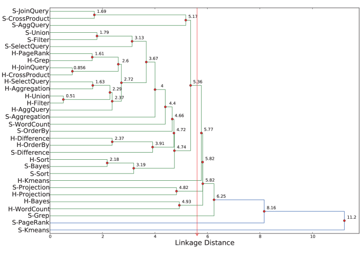
Figure 1: Similarity of Hadoop (H) and Spark (S) workloads.

Figure 1 shows the dendrogram for all big data workloads characterized in this paper. We create the dendrogram by applying PCA and hierarchical clustering to the metrics in Table II. The dendrogram illustrates how each cluster is composed by drawing a U-shaped link between a non-singleton cluster and its children. The length of the top of the U-link is the distance between its children. The shorter the distance, the more similar the children. Like Phansalkar et al. [9], we use Euclidean distance. Further, we use the single linkage distance to create the dendrogram. That is to say the linkage distance between two clusters is made by a single element pair, namely those two elements (one in each cluster) that are closest to each other. In the figure, the x-axis shows the linkage distances among workloads. In our study, we choose eight PCs that have eigenvalues greater than one. These PCs retain 91.12% variance.

We make the following observations from the figure.

Observation 1: At the first clustering iteration, most (80%) of clusters consist of workloads that are based on the same software stack. The only exceptions are S-Bayes/H-Sort and S-Projection/H-Projection with linkage distances of 2.18 and 4.82, respectively. These linkage distances exceed most of the distances between the children in the clusters formed in the first iteration. The shortest linkage distance between the workloads using different software stacks to implement the same algorithm is 3.19 for H-Sort and S-Sort.

Observation 2: Two workloads implementing the same algorithm on different software stacks do not get clustered together in the first clustering iteration — the only exception is Projection. However, the linkage distance between H-Projection and S-Projection is 4.82, which is large enough to indicate that their microarchitectural behaviors are quite different.

Observation 3: After the first iteration, workloads based on the same software stack are easier to cluster together, e.g., S-Union, S-Filter, and S-SelectQuery workloads get clustered together after just two iterations. Likewise, H-SelectQuery, H-Aggregation, H-Union, and H-Filter get clustered after two iterations.

In the dendrogram, when workloads are clustered quickly with small linkage distances, it indicates that the workloads are similar. Workloads based on the same software stack are easier to cluster than programs that implement the same algorithm but use different software stacks because the latter have dramatically different behaviors. We thus conclude that the software stacks have significant impacts on workload behaviors — even greater than that of the benchmark algorithms. This phenomenon occurs because the implementations of the software stacks allow programmers to develop applications without considering system issues. For instance, a Hadoop-based WordCount application has only 50-some lines of user application code in both the Map and Reduce functions. In contrast, Hadoop’s source code can be dozens or even hundreds of megabytes. For example in Hadoop version 1.0.2, the size of the main source code (i.e. src folder size) is 67 MB. The upshot is that the ratio of system software and middleware instructions executed compared to user application instructions tends to be large, which makes their impact on system behavior large, as well.

Observation 4: H-Union/H-Filter, S-Union/S-Filter, H-JoinQuery/H-CrossProduct, and S-JoinQuery/S-CrossProduct, are grouped, respectively, in the first clustering iteration. On an algorithmic level, join query and cross product are similar. Both operate records from two tables at once. Union and filter also perform similar operations in the BigDataBench implementations. From this we conclude that workloads using the same software stack to implement similar algorithms have similar behaviors.

Observation 5: Most of the Hadoop-based workloads exhibit small linkage distances, and thus they are easier to cluster. There are nine Hadoop workloads (H-Pagernak to H-AggQuery in Figure 1) clustered within linkage distances of 2.72. In contrast, only three Spark-based workloads (S-Union to S-SelectQuery in Figure 1) are clustered within a similar distance (3.13). H-Union and H-Filter are clustered with linkage distance of 0.51, and H-JoinQuery and H-CrossProduct are clustered with distance of 0.856. In contrast, S-Union and S-Filter get grouped with linkage distance of 1.79, and S-JoinQuery and S-CrossProduct are clustered with distance of 1.69.

The above observation shows that Hadoop-based workloads have more similarities with each other than their Spark-based counterparts. We thus conclude that Hadoop has a larger impact on microarchitectural behaviors than Spark. Its software stack dominates application behavior, minimizing the impact of potentially diverse behaviors introduced by user application code. Spark is simpler than Hadoop with respect to number of lines of code, and thus it dominates system behavior less. For instance, in contrast to Hadoop’s source code size, Spark’s whole folder is only 11 MB for version 0.81.

The bottom line is that software stacks play an important role in big data systems, and that impact may increase over time. As more and more mechanisms and services are added, software stacks become more and more complicated. Taking the tar package as an example, its size in Hadoop version 1.0.2 was 32.6MB, whereas in version 2.4, its size grows to 133MB. The impact of software stacks to application behaviors may become greater and greater. Thus to choose representative workloads to benchmark big data systems, the software stack should be considered separately from the algorithms in user application code, and different software stacks should be included for thorough workload characterization.

V-B Principle Component Space Analysis

In this section, we project the workloads into principle component spaces. We only present the first four PCs covering 71.45% of the total variance due to space limitations. Figure 2 shows the scatter plot of the first and second principle components, PC1 and PC2. Figure 3 shows this for PC3 and PC4. These visualizations only include a subset of available information based on the first four PCs. Workloads appearing close in these figures may in fact be farther away when all PCs are considered. Even in this subset, however, workloads that appear far apart indeed exhibit significantly different behaviors.

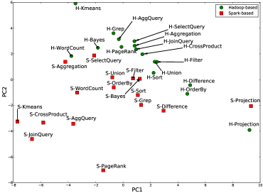
Figure 2: Scatter plot of workloads using the first and second principle components

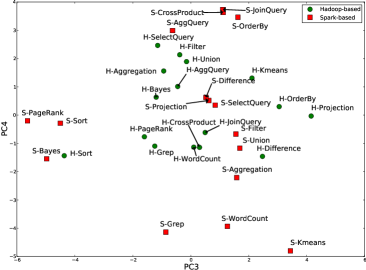
Figure 3: Scatter plot of workloads using the third and fourth principle components

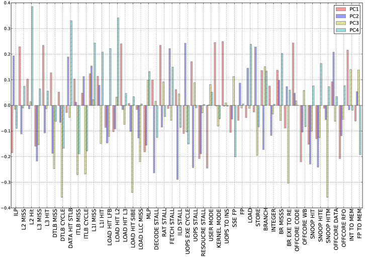
Figure 4: Factor loadings for all workloads

The factor loadings can show the map from the original microarchitecture level metrics to the principle components. Figure 4 shows the factor loadings of the first four PCs. This means that the PC1 is computed as $PC1=-0.18\times ILP+0.23\times L2~{}MISS+0.102\times L2~{}HIT+...$. PC1 is positively dominated by L2 MISS, L3 HIT, LOAD HIT L3, RAT STALL, KERNEL MODE, UOPS TO INS, OFFCORE CODE, and INT TO MEM. And PC1 is also negatively dominated by RESOURCE STALL, USER MODE, OFFCORE WB, and OFFCORE RFO. That is to say, when compared with other workloads, the workloads in Figure 2 with a high value along PC1, have more L2 MISS, L3 HIT, LOAD HIT L3, RAT STALL, KERNEL MODE instructions, OFFCORE CODE requests, higher UOPS TO INS ratio and INT TO MEM ratio. At the same time they have less RESOURCE STALL, USER MODE instructions, OFFCORE WB, and OFFCORE RFO requests. Similarly, Figure 4 also shows the factors that positively or negatively dominate the other three PCs. The factor loadings can also help us to understand the behavior differences among workloads. Such as H-Kmeans has highest value along PC2 (Figure 2) for it has more STORE instructions, FETCH STALL, and DATA HIT STLB. S-Kmeans, S-WordCount, and S-Grep discriminate themselves along PC4 (Figure 3) due to their low L2 HIT rates, STLB HIT rates, L1 instruction hit rates, percentages of LOAD instructions, and branch miss rates and their high ITLB miss rates and more ITLB walk cycles. Factor loadings also explain the other isolated points in a similar way, but we omit them for brevity.

The Spark-based workloads are spread widely along the x-axis (PC1) in Figure 2. In contrast, the Hadoop-based workloads are grouped in the middle of the chart. The Spark-based workloads thus exhibit more diversity than their Hadoop-based counterparts with respect to PC1. Figure 3 displays similar phenomena. The Spark-based workloads nearly cover all of the space for PC3 and PC4, whereas the Hadoop-based workloads are again grouped in the center. There are some isolated points in the figures, most of which represent Spark-based workloads exhibiting behaviors that differ from the other workloads. These phenomena verify our finding in Section V-A that the Spark-based workloads show more diversity than the Hadoop-based workloads with respect to microarchitectural behaviors because the Hadoop software stack minimizes the impact of the user application code.

V-C Differentiating Hadoop and Spark

On the y-axis (PC2) in Figure 2 we find that most of the Hadoop-based workloads are located towards the top, whereas most of Spark-based workloads are located in the middle or bottom parts of the chart. Spark-based workloads and Hadoop-based workloads are mixed along other PC dimensions. So we conclude that PC2 is the main component that differentiates the Hadoop-based workloads from the Spark-based workloads. We therefore investigate which microarchitectural-level metrics dominate PC2 values. Figure 4 shows the weights of each microarchitecture metric for PC1-PC4. The metrics that negatively dominate PC2’s values are L3 MISS, DTLB MISS, DECODE STALL, ILD STALL, UOPS STALL, RESOURCE STALL, BRANCH, SNOOP HIT, and SNOOP HITE. The metrics that positively dominate its values are ILP, DAT HIT STLB, FETCH STALL, UOPS EXE CYCLE, STORE, and OFFCORE DATA. We therefore compare the workloads using those metrics.

Figure 5 shows the main metrics that dominate PC2’s values. We calculate the mean for each metric for each kind of big workload and present normalized Hadoop-based values using the Spark-based workloads as the baseline. In the figure, the metrics that have negative impact have lower values for the Hadoop-based workloads, whereas those with positive impact have higher values. Most of the Hadoop-based workloads have higher PC2 values than their Spark-based counterparts.

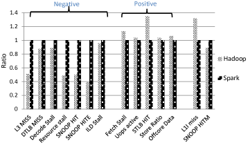
Figure 5: Metrics causing Hadoop and Spark to behave differently

We make the following observations from Figure 5.

Observation 6: The Spark-based workloads have a large amount of L3 cache misses per kilo instructions, about twice those of the Hadoop-based workloads.

Observation 7: The Hadoop-based workloads have more data shared TLB hits and fewer DTLB misses than the Spark-based workloads.

Observation 8: The Hadoop-based workloads have more instruction fetch stalls, whereas the Spark-based workloads have more resource related stalls.

We can divide the processor architecture into two parts: the in-order frontend, which fetches, decodes, and issues instructions, and the out-of-order backend, which executes instructions and writes data back to the register file. The instruction fetch stalls belong to the frontend and the resource related stalls belong to the backend. The former are mainly caused by L1 instruction cache misses. Figure 5 shows that the L1 I-cache misses per kilo instructions (MPKI) are about 30% higher for the Hadoop-based workloads on average.

Most resource stalls (e.g., load/store buffer full and reservation station full) are likely caused by long latency L3 data cache or data TLB misses. Note that in our processor, an STLB (second level Shared TLB) hit implies an L1 TLB miss. In Figure 5, the DTLB miss metric includes both levels. The Hadoop-based workloads have more data STLB hits, which means that the data STLB is more efficient for those workloads. We confirm that by calculating the data STLB hit rates. The data STLB hit rate is 61.48%, on average, for Hadoop-based workloads, whereas the rate for their Spark-based counterparts is 50.80%, on average.

In general, the large number of L3 cache and data TLB misses cause more backend stalls for the Spark-based workloads, and the high instruction cache misses cause more frontend stalls for the Hadoop-based workloads. We conclude that the Hadoop-based workloads have larger instruction footprints than their Spark-based counterparts. These phenomena could be because larger application binaries (including the software stacks) create more I-cache misses [28, 5], especially in the case of Hadoop. However the Spark-based workloads have larger data footprints than Hadoop-based workloads. This may be caused by the different operation modes on intermediate data between Hadoop and Spark software stacks.

Observation 9: The Spark-based workloads have more SNOOP HIT and SNOOP HITE responses than Hadoop-based workloads.

Both responses represent coherence traffic among different cores, so they reflect data sharing patterns. The Spark-based workloads also have more SNOOP HITM responses. These metrics show that Spark-based workloads have more data sharing among different cores.

As the number of cores increases, the traffic caused by the cache coherence protocol will increase. Programmers and architects should thus pay much attention to data sharing (particularly false sharing) in Spark-based workloads. This implies that different software stacks will require different optimization strategies or lead to different system design decisions: there is no single solution.

VI Subsetting

Computer architects often use benchmark suite subsets that capture the most important system behaviors [7]. This approach reduces simulation and evaluation time, and thus shortens the research period. A well selected subset can reduce workload redundancy while keeping representativity. Here we use the data obtained from Section V to eliminate redundant workloads and generate a representative subset of BigDataBench. Note that both the previous section’s similarity analyses and this section’s subsetting are all from a computer architecture point of view. Results may differ if subsetting is performed from a different point of view [29].

Statistical approaches are frequently used to facilitate workload subsetting. In this section we use PCA and clustering analysis to remove the redundant workloads similarly to previous efforts [6, 9, 30].

VI-A Clustering

We use clustering on the eight principle components obtained from the PCA algorithm to group workloads into similarly behaving application clusters (the eight PCs are those in Section V). In particular, we use K-Means clustering for a number of K values. Inspired by previous research [30, 31], we use the Bayesian Information Criterion (BIC) to choose the proper K value. The BIC is a measure of the “goodness of fit” of a clustering for a data set. The larger the BIC scores, the higher the probability that the clustering is a good fit to the data. Here we determine the K value that yields the highest BIC score. We use the formulation from Pelleg et al. [32] shown in Equation 1 to calculate the BIC.

$$BIC(D,K)=l(D|K)-\frac{{p}_{j}}{2}log(R)$$ (1)

Where $D$ is the original data set to be clustered. In this paper, $D$ is $32\times 8$ matrix which indicates $32$ workloads and each workload is represented by $8$ PCs (Principle Components). $l(D|K)$ is the likelihood. $R$ is the number of workloads to be clustered. $p_{j}$ is the sum of $K-1$ class probabilities, which is $K+dK$. $d$ is the dimension of each workloads, which is $8$ in this paper for we choose $8$ PCs. To compute $l(D|K)$, we use Equation 2.

$$l(D|K)=\sum{{}^{K}_{i=1}}(-\frac{{R}_{i}}{2}log(2\pi)-\frac{{R}_{i}\cdot d}{2}log(\sigma^{2})$$ (2)

$$-\frac{R_{i}-K}{2}+R_{i}logR_{i}-R_{i}logR)$$

Where $R_{i}$ is the number of points in the $i^{th}$ cluster, and $\sigma^{2}$ is the average variance of the Euclidean distance from each point to its cluster center, which is calculate by Equation 3.

$$\sigma^{2}=\frac{1}{R-K}\sum_{i}(x_{i}-\mu(i))^{2}$$ (3)

Here $x_{i}$ is the data point assigned to cluster $i$, and $\mu(i)$ represents the center coordinates of cluster $i$.

We ultimately cluster the 32 workloads into seven groups which are listed in Table IV. Please note that though the result of K-Means is similar to that of hierarchical clustering in Figure 1, the K-Means clustering can not measure the similarity among different workloads quantitatively like the hierarchical clustering. For example, the hierarchical clustering measures that H-Projection and S-Projection are clustered together with a linkage distance of 4.82, while the K-Means can only indicate that they are clustered together qualitatively.

TABLE IV: The result of K-Means Clustering Algorithm

Cluster	Workloads	Number
1	H-PageRank, H-Grep, H-JoinQuery, H-Sort, H-CrossProduct, S-Bayes, S-Grep, S-Sort	8
2	H-AggQuery, S-Filter, S-Union, S-SelectQuery, S-OrderBy, H-Kmeans	6
3	S-Aggregation, S-WordCount, S-Kmeans, H-Wordcount, H-Bayes	5
4	H-OrderBy, H-Difference, S-Difference, S-PageRank	4
5	H-Aggregation, H-Filter, H-Union, H-SelectQuery	4
6	S-CrossProduct, S-JoinQuery, S-AggQuery	3
7	H-Projection, S-Projection	2

VI-B Selecting Representative Workloads

The representative for each cluster can be chosen by two approaches, as mentioned by Eeckhout et al. [6]. The first is to choose the workload that is as close as possible to the center of the cluster it belongs to. The other is to select an extreme workload situated at the “boundary” of each cluster. We experiment with both approaches. Table V lists the representative workloads selected from each cluster by both approaches.

The third column of Table V gives the maximal linkage distance among representative workloads for each approach. We find that workloads chosen by the first approach do not cover workloads with long linkage distances, e.g., S-PageRank. The maximal distance among representative workloads selected by the first approach is smaller than the maximal distance among those selected by the second approach. This means that workloads chosen by the first method are not as diverse as the second approach does.

In Section V we perform hierarchical clustering to analyze workload similarity. To use hierarchical clustering to select seven representative workloads, we just draw a vertical line at a point close to 5.6 for the vertical line is intersecting with seven horizontal lines in Figure 1. There are four single workload consisted clusters have intersections with the vertical line. This reveals that we should choose those four workloads, namely, S-PageRank, S-Kmeans, S-Grep, and H-Kmeans. These four workloads are also chosen by the second approach, whereas none of them is chosen by the first approach. We therefore deem the second approach superior in selecting representative workloads. And the rationale behind this method can be that the behaviors of other workloads in the cluster can be extracted from the behavior of the boundary one, e.g. through interpolation  [6].

TABLE V: Representative workloads chosen by different approaches

Approach	Representatives Workloads	Maximal Linkage Distance
Nearest to	H-PageRank (8)
Cluster Center	S-Select (6)
	S-Aggregation (5)
	S-Difference (4)	5.82
	H-Aggregation (4)
	S-CrossProduct (3)
	S-Projection (2)
Farthest from	S-Grep (8)
Cluster Center	H-Kmeans (6)
	S-Kmeans (5)
	S-PageRank (4)	11.20
	H-SelectQuery (4)
	S-AggQuery (3)
	H-Projection (2)

The number of workloads that the selected workloads can represent are given in parentheses.

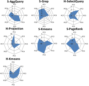
Figure 6: Kiviat diagrams of the representative workloads

Figure 6 shows Kiviat diagrams for the representative workloads chosen by the second approach. The diagrams illustrate that the representative workloads are diverse and that different workloads are dominated by different principle components.

VI-C BigDataBench Simulator Version

We deploy the representative applications on a full-system simulator and release the simulator images as the BigDataBench simulator version. More information can be found on the project web page http://prof.ict.ac.cn/BigDataBench/simulatorversion/. For the big data workloads change frequently [33], the state-of-art workloads and software stacks will be integrated into and out-of-date ones will be removed from BigDataBench. We will continue the subsetting work, so the BigDataBench simulator version on the web site may be different from the one mentioned in this paper when you access the web site. It is our hope that this simulator version will benefit architecture researchers by reducing the costs of evaluating alternative technological approaches in big data systems.

VII Related Work

Wang et al. [11] propose a comprehensive big data workloads suite, including different structured, un-structured, and semi-structured data. However, a large number of benchmarks pose great challenges, since our usual simulation-based research methods become prohibitively expensive. Xi et al. [34] characterize micro architecture level behaviors of the search engine. Ferdman et al. [5] select seven scale-out workloads according to popularity. They use hardware performance counters to analyze microarchitectural behaviors of those scale-out workloads. They compare the scale-out workloads and traditional benchmarks to identify the key contributors to the microarchitecture inefficiency on modern processors. They conclude that mismatches exist between the needs of scale-out workloads and the capabilities of modern processors. Jia et al. [28, 35] characterize microarchitectural characteristics of data analysis workloads, also finding that they exhibit different characteristics from traditional workloads. Luo et al. [36] compare two clusters’ performance and power consumption using hybrid big data workloads. Continuing the work in  [36], our group also releases the multi-tenancy version of BigDataBench, which support the scenarios of multiple tenants running heterogeneous applications in the same datacenter. The multi-tenancy version of BigDataBench is publicly available from [37], which is helpful for the research of datacenter resource management and other interesting issues [38, 39].

Much work focuses on comparing the performance of different data management systems. For OLTP or database systems evaluation, TPC-C [40] is often used to evaluate transaction-processing system performance in terms of transactions per minute. Cooper et al. [41] define a core set of benchmarks and report throughput and latency results for five widely used data management systems. Pavlo et al. [42] compare the MapReduce paradigm to traditional parallel DBMS platforms. The Berkeley AMPLab Big Data Benchmark [4] can also be used to compare MapReduce and parallel DBMS platforms in terms of response time for a handful of relational queries across different data sizes.

Many prior studies characterize benchmarks via statistical data analysis techniques such as PCA and clustering. For instance, Eeckhout et al. [6, 8], Phansalkar et al. [9, 43], and Yi et al. [7] all employ statistical analyses to characterize workloads, analyze redundancy, and perform subsetting for general-purpose and embedded benchmark suites. Our work here is inspired by their methods, although we focus on a very different application domain.

VIII Conclusion

Achieving benchmark comprehensiveness while enabling efficient experimentation raises great challenges for the architecture community, in general, and the problem is particularly acute in big data systems research. The diversity of big data software stacks aggravates the challenge, especially for simulation-based research. Here we use 45 microarchitectural metrics to characterize 32 big data workloads on two different software stacks. Our statistical analyses on the gathered metrics reveal that software stacks have significant impacts on workload behavior, and we find that in the context of our experiments, this impact is greater than that of the algorithms employed in user application code.

In order to facilitate simulation-based research, we create a streamlined, representative subset of the benchmarks in the BigDataBench suite. To do so, we remove the redundant workloads via K-Means clustering. In order to choose the best K value for the K-Means algorithm, we use BIC as the statistical test method to evaluate the K-Means efforts. After subsetting, we are left with some representative workloads. Our hope is that our subsetting approach and resulting benchmark suite will enable more architecture researchers to study alternative organizations and technologies for big data systems.

References

- [1] E. Schmidt, “Techonomy conference,” http://techcrunch.com/2010/08/04/schmidt-data/, cited Apr. 2014.
- [2] G. John and R. David, “THE DIGITAL UNIVERSE IN 2020: Big Data, Bigger Digital Shadows, and Biggest Growth in the Far East,” IDC Report, 2012.
- [3] M. Zaharia, M. Chowdhury, T. Das, A. Dave, J. Ma, M. McCauley, M. J. Franklin, S. Shenker, and I. Stoica, “Resilient distributed datasets: A fault-tolerant abstraction for in-memory cluster computing,” in USENIX Conference on Networked Systems Design and Implementation, 2012.
- [4] “Big Data Benchmark.” https://amplab.cs.berkeley.edu/benchmark/, cited Apr. 2014.
- [5] M. Ferdman, A. Adileh, O. Kocberber, S. Volos, M. Alisafaee, D. Jevdjic, C. Kaynak, A. Popescu, A. Ailamaki, and B. Falsafi, “Clearing the clouds: A study of emerging workloads on modern hardware,” Architectural Support for Programming Languages and Operating Systems, Mar. 2012.
- [6] L. Eeckhout, H. Vandierendonck, and K. De Bosschere, “Quantifying the impact of input data sets on program behavior and its applications,” Journal of Instruction-Level Parallelism, vol. 5, no. 1, pp. 1–33, 2003.
- [7] J. J. Yi, R. Sendag, L. Eeckhout, A. Joshi, D. J. Lilja, and L. K. John, “Evaluating benchmark subsetting approaches,” in IEEE International Symposium on Workload Characterization, Oct. 2006, pp. 93–104.
- [8] L. Eeckhout, H. Vandierendonck, and K. De Bosschere, “Workload design: Selecting representative program-input pairs,” in International Conference on Parallel Architectures and Compilation Techniques, Sep. 2002, pp. 83–94.
- [9] A. Phansalkar, A. Joshi, and L. John, “Analysis of redundancy and application balance in the SPEC CPU2006 benchmark suite,” in International Symposium on Computer Architecture, Jun. 2007.
- [10] T. White, Hadoop: The Definitive Guide. O’Reilly Media, 2009.
- [11] L. Wang, J. Zhan, C. Luo, Y. Zhu, Q. Yang, Y. He, W. Gao, Z. Jia, Y. Shi, S. Zhang et al., “BigDataBench: A big data benchmark suite from internet services,” in IEEE International Symposium on High Performance Computer Architecture, 2014.
- [12] J. Gray, Benchmark Handbook: for Database and Transaction Processing Systems. Morgan Kaufmann Publishers Inc., 1992.
- [13] C. Bienia, S. Kumar, J. Singh, and K. Li, “The PARSEC benchmark suite: Characterization and architectural implications,” in International Conference on Parallel Architectures and Compilation Techniques, Oct. 2008, pp. 72–81.
- [14] Y. Chen, F. Raab, and R. Katz, “From tpc-c to big data benchmarks: A functional workload model,” in Specifying Big Data Benchmarks. Springer, 2014, pp. 28–43.
- [15] P. Wang, D. Meng, J. Han, J. Zhan, B. Tu, X. Shi, and L. Wan, “Transformer: A new paradigm for building data-parallel programming models,” IEEE Micro, vol. 30, no. 4, pp. 55–64, 2010.
- [16] Z. Ming, C. Luo, W. Gao, R. Han, Q. Yang, L. Wang, and J. Zhan, “BDGS: A scalable big data generator suite in big data benchmarking,” Lecture Note in Computer Sciences, Extended Version for the Fourth Workshop on Big Data Benchmarking, 2014.
- [17] A. Thusoo, J. S. Sarma, N. Jain, Z. Shao, P. Chakka, S. Anthony, H. Liu, P. Wyckoff, and R. Murthy, “Hive: A warehousing solution over a map-reduce framework,” the VLDB Endowment, vol. 2, no. 2, pp. 1626–1629, 2009.
- [18] C. Engle, A. Lupher, R. Xin, M. Zaharia, M. J. Franklin, S. Shenker, and I. Stoica, “Shark: Fast data analysis using coarse-grained distributed memory,” in ACM SIGMOD International Conference on Management of Data, May 2012, pp. 689–692.
- [19] T. S. Karkhanis and J. E. Smith, “A first-order superscalar processor model,” in International Symposium on Computer Architecture, Jun. 2004, pp. 338–349.
- [20] K. Keeton, D. A. Patterson, Y. Q. He, R. C. Raphael, and W. E. Baker, “Performance characterization of a Quad Pentium Pro SMP using OLTP workloads,” in International Symposium on Computer Architecture, Jun. 1998.
- [21] S. Eyerman, L. Eeckhout, T. Karkhanis, and J. E. Smith, “A performance counter architecture for computing accurate CPI components,” in International Conference on Architectural Support for Programming Languages and Operating Systems, Oct. 2006, pp. 175–184.
-
[22]
D. Levinthal, “Cycle accounting analysis on Intel Core 2 processors,”
https://software.intel.com/sites/products/collateral/hpc/vtune/
cycle_accounting_analysis.pdf, cited Apr. 2014. - [23] I. Jolliffe, Principal Component Analysis. Wiley Online Library, 2005.
- [24] C. Bienia and K. Li, “Fidelity and scaling of the PARSEC benchmark inputs,” in IEEE International Symposium on Workload Characterization, Dec. 2010, pp. 1–10.
- [25] D. Levinthal, “Performance Analysis Guide for Intel Core i7 Processor and Intel Xeon 5500 Processors,” Intel Performance Analysis Guide, 2009.
- [26] “Performance counters for linux,” https://perf.wiki.kernel.org/index.php, cited Apr. 2014.
- [27] Programming Guide, “Intel® 64 and IA-32 architectures software developer’s manual,” 2011.
- [28] Z. Jia, L. Wang, J. Zhan, L. Zhang, and C. Luo., “Characterizing data analysis workloads in data centers,” in IEEE International Symposium on Workload Characterization, Sep. 2013.
- [29] R. M. Yoo, H.-H. Lee, H. Lee, and K. Chow, “Hierarchical means: Single number benchmarking with workload cluster analysis,” in IEEE International Symposium on Workload Characterization, Sep. 2007, pp. 204–213.
- [30] K. Hoste and L. Eeckhout, “Comparing benchmarks using key microarchitecture-independent characteristics,” in IEEE International Symposium on Workload Characterization, Oct. 2006, pp. 83–92.
- [31] T. Sherwood, E. Perelman, G. Hamerly, and B. Calder, “Automatically characterizing large scale program behavior,” in International Conference on Architectural Support for Programming Languages and Operating Systems, Oct. 2002.
- [32] D. Pelleg and A. W. Moore, “X-means: Extending K-means with efficient estimation of the number of clusters.” in International Conference on Machine Learning, Jun. 2000, pp. 727–734.
- [33] L. Barroso and U. Hölzle, “The datacenter as a computer: An introduction to the design of warehouse-scale machines,” Synthesis Lectures on Computer Architecture, vol. 4, no. 1, pp. 1–108, 2009.
- [34] H. Xi, J. Zhan, Z. Jia, X. Hong, L. Wang, L. Zhang, N. Sun, and G. Lu, “Characterization of real workloads of web search engines,” in IEEE International Symposium on Workload Characterization, Nov. 2011, pp. 15–25.
- [35] Z. Jia, R. Zhou, C. Zhu, L. Wang, W. Gao, Y. Shi, J. Zhan, and L. Zhang, “The implications of diverse applications and scalable data sets in benchmarking big data systems,” in Specifying Big Data Benchmarks. Springer, 2014, pp. 44–59.
- [36] C. Luo, J. Zhan, Z. Jia, L. Wang, G. Lu, L. Zhang, C. Xu, and N. Sun, “Cloudrank-d: benchmarking and ranking cloud computing systems for data processing applications,” Frontiers of Computer Science, vol. 6, no. 4, pp. 347–362, 2012.
- [37] “BigDataBench multi-tenancy version,” http://prof.ict.ac.cn/BigDataBench/multi-tenancyversion/, cited Apr. 2014.
- [38] L. Wang, J. Zhan, W. Shi, and Y. Liang, “In cloud, can scientific communities benefit from the economies of scale?” IEEE Transactions on Parallel and Distributed Systems, vol. 23, no. 2, pp. 296–303, 2012.
- [39] J. Zhan, L. Wang, X. Li, W. Shi, C. Weng, W. Zhang, and X. Zang, “Cost-aware cooperative resource provisioning for heterogeneous workloads in data centers,” IEEE Transactions on Computers, vol. 62, no. 11, pp. 2155–2168, 2013.
- [40] “TPC-C,” http://www.tpc.org/tpcc, cited Apr. 2014.
- [41] B. Cooper, A. Silberstein, E. Tam, R. Ramakrishnan, and R. Sears, “Benchmarking cloud serving systems with YCSB,” in ACM Symposium on Cloud Computing, Jun. 2010, pp. 143–154.
- [42] A. Pavlo, E. Paulson, A. Rasin, D. J. Abadi, D. J. DeWitt, S. Madden, and M. Stonebraker, “A comparison of approaches to large-scale data analysis,” in ACM SIGMOD International Conference on Management of Data, Jun. 2009, pp. 165–178.
- [43] A. Phansalkar, A. Joshi, and L. K. John, “Subsetting the SPEC CPU2006 benchmark suite,” ACM SIGARCH Computer Architecture News, vol. 35, no. 1, pp. 69–76, 2007.