The star formation history of the Magellanic Clouds derived from long-period variable star counts

Abstract

We present the first reconstruction of the star formation history (SFH) of the Large and Small Magellanic Clouds (LMC and SMC) using Long Period Variable stars. These cool evolved stars reach their peak luminosity in the near-infrared; thus, their K-band magnitudes can be used to derive their birth mass and age, and hence the SFH can be obtained. In the LMC, we found a 10-Gyr old single star formation epoch at a rate of $\sim 1.5$ M_⊙ yr^-1, followed by a relatively continuous SFR of $\sim 0.2$ M_⊙ yr^-1, globally. In the core of the LMC (LMC bar), a secondary, distinct episode is seen, starting 3 Gyr ago and lasting until $\sim 0.5$ Gyr ago. In the SMC, two formation epochs are seen, one $\sim 6$ Gyr ago at a rate of $\sim 0.28$ M_⊙ yr^-1 and another only $\sim 0.7$ Gyr ago at a rate of $\sim 0.3$ M_⊙ yr^-1. The latter is also discernible in the LMC and may thus be linked to the interaction between the Magellanic Clouds and/or Milky Way, while the formation of the LMC bar may have been an unrelated event. Star formation activity is concentrated in the central parts of the Magellanic Clouds now, and possibly has always been if stellar migration due to dynamical relaxation has been effective. The different initial formation epochs suggest that the LMC and SMC did not form as a pair, but at least the SMC formed in isolation.

1 Introduction

The Magellanic Clouds (Large, LMC, and Small, SMC) are irregular, gas-rich dwarf galaxies in our Local Group. The presence of a bar-like structure – especially prominent in the LMC – suggests that they could have originally been barred spiral galaxies transformed into present-day irregular galaxies due to their tidal interactions with one another and with the Milky Way. At a distance of 48.5 kpc (Macri et al. 2006; Freedman et al. 2010), the LMC is the third closest galaxy to the Milky Way. With an inclination of $32^{\circ}$ (Haschke et al. 2011) it offers us an excellent view of its structure and content. The SMC is located at a distance of $\sim 61$ kpc (Hilditch et al. 2005) with an inclination of only $2.6^{\circ}$ (Subramanian et al. 2011).

Probing the star formation history (SFH) in galaxies informs us about galaxy formation and evolution. Star clusters revealed differences in the SFH between the LMC and the Milky Way (Hodge 1960; Sagar & Pandey 1989): the LMC contains a larger fraction of young clusters relative to the Milky Way. Other methods of determining the SFH include a comparison of the observed Colour–Magnitude Diagrams (CMDs) with the model-built CMDs (e.g., Bertelli et al. 1992). Harris & Zaritsky (2009) used multi-color photometry of millions of stars over $\approx 65$ deg² of the LMC to derive the SFH; they found multiple episodes of star formation between 5 to 0.1 Gyr ago in addition to an initial burst of star formation $\sim 12$ Gyr ago. In a recent study, Cignoni et al. (2013) studied various fields within the bar and wing of the SMC and confirmed a dominant intermediate-age star formation epoch. Their derived metallicity for the fields support a well mixed metal content of the SMC. The CMD approach has also revealed that the most recent star formation, as young as $\approx 100$ Myr, is confined to the central regions in both the LMC and SMC (Indu & Subramanian 2011).

Our approach to investigate the SFH is based on employing Long Period Variable stars (LPVs). These are mostly Asymptotic Giant Branch (AGB) stars at their very late stage of evolution, as well as more massive red supergiants (RSGs). The AGB stars alone have low- to intermediate-mass ranges which relate to diverse ages and hence time epochs in the past, and they can thus be used to derive Star Formation Rates (SFRs) over much of a galaxy’s cosmological evolution. The AGB stars develop unstable mantles which cause radial pulsation at periods of one or a few years; they are luminous ($\sim 10^{4}$ L_⊙) and cool ($<4000$ K) and hence stand out at near-infrared wavelengths. Their colours can be further reddened by enhanced atmospheric opacity due to carbon-dominated chemistry (in carbon stars) or due to attenuation by circumstellar dust produced in their winds. Thanks to recent large-scale, extended monitoring projects such as OGLE-I, II, III, MACHO and others, we are now in a position to use LPVs to study these nearby galaxies.

The data and the methodology are described in Section 2. In Section 3 we present our analysis and the results. In Section 4 we present the SFH derived from our analysis. Section 5 presents a discussion of the findings and a comparison with other studies. Section 6 contains a summary and conclusions.

2 Data and Methodology

In this paper, we use the catalogue of LPVs in the LMC from Spano et al. (2011) and in the SMC from Soszyński et al. (2011). In the case of the LMC, they used the EROS-2 survey which started functioning efficiently from 1996; it employed two cameras enabling observations at two wavelengths, blue (BE) and red (RE), simultaneously. After seven years of monitoring, it provided a database of 856,864 variables in the LMC of which 43,551 are considered LPVs (Spano et al. 2011). The EROS-2 survey covered an area of 88 deg² on the LMC, which is a superior coverage in comparison with other projects such as MACHO and OGLE-III which covered areas on the LMC of 13.5 deg² and 40 deg², respectively.

Spano et al. cross-identified the EROS-2 LPV candidates with variable stars from the OGLE-III and MACHO surveys. They found nearly 60% of LPVs in common between EROS-2 and MACHO; the difference is attributed to differences in sky coverage between the surveys (Spano et al. 2011). For the SMC, Soszyński et al. used the OGLE-III project which has monitored an area of 14 deg² on the SMC. After 13 years of monitoring in the optical V- and near-infrared I-band, the OGLE survey has provided a database of about 6 million stars in the SMC of which 19,384 are identified as LPVs are detected (Soszyński et al. 2011).

As mentioned, AGB stars become surrounded by dust, which causes reddening and makes them particularly faint in optical bands. Therefore, infrared (IR) studies are preferred. For a comparison and more detailed study of the core region we also utilise Ita et al.’s (2004a) data of variable stars in the Magellanic Clouds. This catalogue had been obtained by cross-identifying the OGLE-II and SIRIUS data (simultaneously observated in J-, H-, and K-band). The total area covered by the SIRIUS survey is 3 deg² and 1 deg² in the LMC and SMC, respectively, covering the core region of these galaxies – in particular, the bar of the LMC (see Fig. 1). Spano et al. (2011) cross-matched the EROS-2 survey with 2MASS near-IR (and Spitzer mid-IR) data, within a search radius of $1^{\prime\prime}$. For the SMC, we cross-matched the original catalogue of Soszyński et al. (2011) with 2MASS, also within a search radius of $1^{\prime\prime}$.

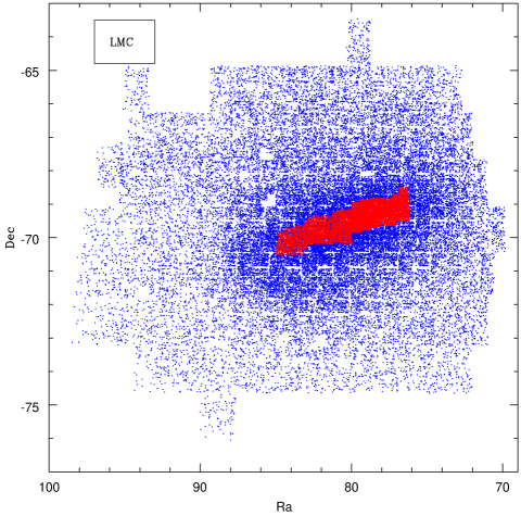
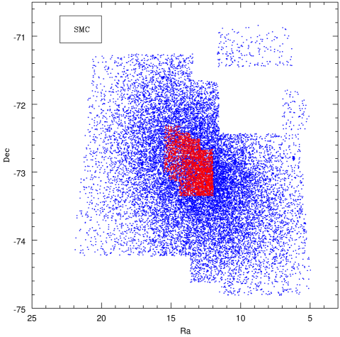
Figure 1: Left: spatial coverage of the Spano et al. (2011) survey (blue) and Ita et al. (2004a) survey (red) in the LMC. Right: spatial coverage of the Soszyński et al. (2011) survey (blue) and Ita et al. (2004a) survey (red) in the SMC.

Ita et al. classified the variable stars into nine groups for the LMC and eight groups for the SMC, based on their location in the period–K-band magnitude plane. The categories include Cepheids, Miras, semi regulars, irregular variables and eclipsing binaries (Ita et al. 2004a). In total, the number of variable stars in Ita’s catalogues of the LMC and SMC are 8852 and 2927, respectively. For the purpose of this study, we select LPVs pulsating in the fundamental mode, equal to sequences C and D in Ita et al. (2004a) above the (first ascent) Red Giant Branch (RGB) tip ($K\sim 12$ and $\sim 12.7$ mag for the LMC and SMC, respectively). Spano et al. (2011) classified their variable stars using period–luminosity relations ($\log P$–$K$ diagram), into six groups (Figs. 22 and 23 in their paper), from which sequence C is considered as Miras pulsating in the fundamental mode. Sequence D comprises mostly of stars with secondary long periods that are probably not due to the same radial pulsation we are after, but it does contain some dusty LPVs that have lengthened pulsation periods as a result of diminished mass (Ita et al. 2004b; Spano et al. 2011). For the purpose of this study we select variables belonging to sequence C, and variables with ”only” one period in sequence D.

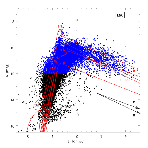
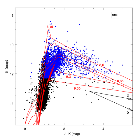
Figure 2: CMD of the LMC (left) and SMC (right), overlain with Marigo et al. (2008) isochrones (labelled by logarithmic age in yr) ; among with circumstellar reddening vectors for oxygenous and carbonaceous dust (O and C, respectively), explained in Section 3.1.1. Blue points are stars above the RGB-tip.

An appropriate stellar evolution model is provided by the Padova group (Marigo et al. 2008). LPVs are expected to be at the end-points of the AGB (or RSG) part of the isochrones in CMDs. Thus, the Padova isochrones were fitted to the CMDs of the Magellanic Clouds in order to correct the reddened LPVs (see Fig. 2). Two different groups of reddening slopes are seen, those with steeper slopes are associated with those stars surrounded by oxygeneous dust whilst some with shallower slopes are associated with carbonaceous dust. Not all stars are reddened; the correction is applied only to those stars which have $J-K>1.5$ mag.

3 From K-band magnitude to the star formation history

The total mass of stars formed between $t$ and $t+{\rm d}t$ depends on star formation rate, $\xi(t)$, as

$${\rm d}M(t)\ =\ \xi(t)\,{\rm d}t.$$ (1)

Thus, $N$, the number of stars formed, is defined by the following equation:

$${\rm d}N(t)\ =\ \left[\frac{\int_{\rm min}^{\rm max}f_{\rm IMF}(m)\,{\rm d}m}{\int_{\rm min}^{\rm max}f_{\rm IMF}(m)m\,{\rm d}m}\right]\,{\rm d}M(t),$$ (2)

in which $f_{\rm IMF}$ is the initial mass function. The nominator represents the total number of stars within the mass range of $M_{\rm min}$–$M_{\rm max}$, whilst the denominator gives their total mass. Therefore, the fraction refers to the number of stars per mass unit. For the initial mass function, the Kroupa (2001) model was used where we assumed $M_{\rm min}=0.02$ M_⊙ and $M_{\rm max}=200$ M_⊙. The number of stars formed between $t$ and $t+{\rm d}t$ is then obtained as follows:

$${\rm d}n(t)\ =\ \left[\frac{\int_{m(t)}^{m(t+dt)}f_{\rm IMF}(m)\,{\rm d}m}{\int_{\rm min}^{\rm max}f_{\rm IMF}(m)\,{\rm d}m}\right]\,{\rm d}N(t).$$ (3)

Because the large-amplitude, long-period variability only comprises a short phase in the evolution of a star lasting $\delta t$, the number of such variable stars that were formed is reduced to

$${\rm d}n^{\prime}(t)\ =\ \left[\frac{\delta t}{{\rm d}t}\right]\,{\rm d}n(t).$$ (4)

Thus, the final equation for the star formation rate derived from the variable star counts is:

$$\xi(t)\ =\ \left[\frac{\int_{\rm min}^{\rm max}f_{\rm IMF}(m)m\,{\rm d}m}{\int_{m(t)}^{m(t+{\rm d}t)}f_{\rm IMF}(m)\,{\rm d}m}\right]\,\frac{{\rm d}n^{\prime}(t)}{\delta t}.$$ (5)

3.1 From K-band magnitude to age

For reasons that will become clear below, we convert K-band magnitudes into stellar birth mass, first, before converting that into the age of the star. For the latter, we use the following mass–age relation:

$$\log{t\,{\rm[yr]}}\ =\ a\,\log{M\,{\rm[M}_{\odot}{\rm]}}+b,$$ (6)

where $a$ and $b$ are given in Javadi et al. (2011), based on the models from Marigo et al. (2008).

Javadi et al. (2011) give the mass–luminosity (K-band magnitude) relation as

$$\log{M\,{\rm[M}_{\odot}{\rm]}}\ =\ aK+b,$$ (7)

where $K$ is the (extinction-corrected) K-band magnitude and $a$ and $b$ are defined in Table 1 for various ranges of $K$. We use a distance modulus of $\mu=18.5$ mag and $\mu=18.9$ mag for the LMC and SMC, respectively.

Table 1: Mass–luminosity relation, $\log{M\,{\rm[M}_{\odot}{\rm]}}=aK+b$, valid for the Large ($Z=0.008$) and Small ($Z=0.004$) Magellanic Clouds (Javadi et al. 2011).

$Z=0.008$
$a$	$b$	validity range
$-0.840$	12.840	$K\leq 7.332$
$-0.589$	9.391	$7.332<K\leq 8.387$
$-0.188\pm 0.028$	$3.465\pm 0.043$	$8.387<K\leq 8.900$
$-0.142\pm 0.027$	$2.758\pm 0.041$	$8.900<K\leq 9.413$
$-0.188\pm 0.022$	$3.487\pm 0.036$	$9.413<K\leq 9.927$
$-0.501\pm 0.016$	$8.183\pm 0.024$	$9.927<K\leq 10.440$
$-0.248\pm 0.018$	$4.335\pm 0.026$	$10.440<K\leq 10.953$
$-0.128\pm 0.025$	$2.257\pm 0.035$	$K>10.953$
$Z=0.004$
$a$	$b$	validity range
$-0.708$	11.1268	$K\leq 8.734$
$-0.209\pm 0.051$	$3.783\pm 0.077$	$8.734<K\leq 9.140$
$-0.240\pm 0.054$	$4.244\pm 0.078$	$9.140<K\leq 9.545$
$-0.050\pm 0.060$	$1.291\pm 0.091$	$9.545<K\leq 9.951$
$-0.131\pm 0.054$	$2.583\pm 0.083$	$9.951<K\leq 10.356$
$-0.243\pm 0.041$	$4.409\pm 0.057$	$10.356<K\leq 10.762$
$-0.714\pm 0.039$	1$2.310\pm 0.055$	$10.762<K\leq 11.167$
$-0.109\pm 0.043$	$1.932\pm 0.070$	$11.167<K\leq 11.573$
$-0.153\pm 0.046$	$2.690\pm 0.067$	$K>11.573$

3.1.1 Dust correction

The light from the variable stars can be attenuated by interstellar and/or circumstellar dust; this is wavelength dependent resulting also in reddening of the near-IR colours. To determine the intrinsic K-band magnitude, the photometry needs to be de-reddened. The (de-)reddening slope in the CMD depends on whether the dust is oxygenous or carbonaceous in composition. Stars with a birth mass in the range of 1.5–4 M_⊙ are expected to have become carbon stars due to the third dredge-up of nculear-processed material material with a carbon:oxygen ratio in excess of unity. In stars with a birth mass $<1.5$ M_⊙, third dredge-up is not sufficiently efficient, whilst, for stars with a birth mass $>4$ M_⊙ nuclear burning of the carbon at the bottom of the convection zone prevents the surface to be enriched in carbon. The reddening correction equation is

$$K\ =\ K+a(1.25-(J-K)),$$ (8)

where $a$ is the average slope for each dust type.

The procedure followed was to first apply a correction assuming carbonaceous dust. If the mass resulting from this corrected K-band magnitude ended up in the range 1.5–4 M_⊙ then the star was treated as a carbon star. Otherwise, the correction was replaced by one assuming oxygenous dust, and a mass was derived accordingly.

Figure 3 shows the mass histogram for different choices of reddening correction. To appreciate the impact of these choices on the derived SFH, we also applied the reverse approach; assuming that stars are oxygen-rich unless their masses would fall within 1.5–4 M_⊙.

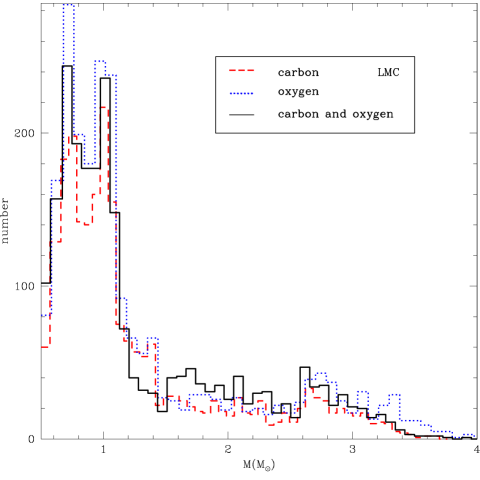
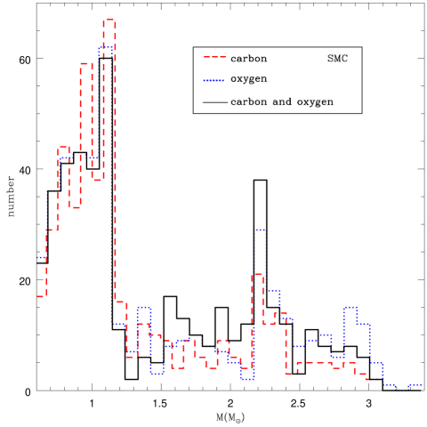
Figure 3: Present day mass function of the LMC (left) and SMC (right). The red dashes are related to carbonaceous correction only, the blue dots are for oxygenous correction only, and the black lines refer to the approach described in the text applying carbonaceous and oxygenous corrections depending on the resulting mass.

3.2 The fraction of the time spent pulsating

Eq. (5) depends on a correction factor ($\delta t$) for the duration of the evolutionary phase in which the star exhibits large-amplitude, long-period pulsations. Generally, since a massive star evolves faster, its pulsation duration is shorter. Thus, low mass stars are more likely to be identified as variables, in comparison to more massive stars. However, the pulsation phase depends sensitively on the star’s effective temperature which, in turn, depends on metallicity, mass loss, et cetera.

Table 2: Parameters adopted for the mass–pulsation relation, $\log(\delta t/t)=D+\sum_{i=1}^{3}a_{i}\exp\left((\log{M\,{\rm[M}_{\odot}{\rm]}}-b_{i})^{2}/(2c_{i}^{2})\right)$, where $\delta t$ is the pulsation duration and $t$ is the age of the star, for the Large ($Z=0.008$) and Small ($Z=0.004$) Magellanic Clouds (Javadi et al. 2011).

$Z=0.008$
$D$	$i$	$a$	$b$	$c$
$-3.96$	1	2.34	1.281	0.378
	2	1.32	0.460	0.165
	3	0.38	0.145	0.067
$Z=0.004$
$D$	$i$	$a$	$b$	$c$
$-4.00$	1	2.29	1.217	0.408
	2	0.84	0.524	0.093
	3	0.87	0.206	0.088

The mass–pulsation relation from Javadi et al. ( 2011) is used to connect the birth mass of stars to their pulsation duration. Relative to its age, it is parameterised as

$$\log\left(\frac{\delta t}{t}\right)\ =\ D+\sum_{i=1}^{3}a_{i}\exp\left[\frac{\left(\log{M\,{\rm[M}_{\odot}{\rm]}}-b_{i}\right)^{2}}{2c_{i}^{2}}\right],$$ (9)

where $a$, $b$, $c$ and $D$ are defined in Table 2.

Given the above argument, the star formation rate estimated using LPVs is shown to be underestimated by a factor of 10 (Javadi et al. 2013) in comparison to the star formation rate obtained using $H_{\alpha}$ emission, for instance. This inaccuracy was exposed by a mismatch between the integrated mass loss and birth mass. To reconcile both the mass loss budget and star formation rate with independent evidence, the pulsation duration adopted from the Marigo et al. (2008) models needs to be decreased by a factor 10. This is a fairly robust result and we thus apply the correction in our work. Given the uncertainties in the models, in particular with regard to the duration of the LPV phase, the star formation rates and stellar masses formed are possibly uncertain by up to a factor of a few.

4 Results and discussion

4.1 The global Star Formation History of the Magellanic Clouds

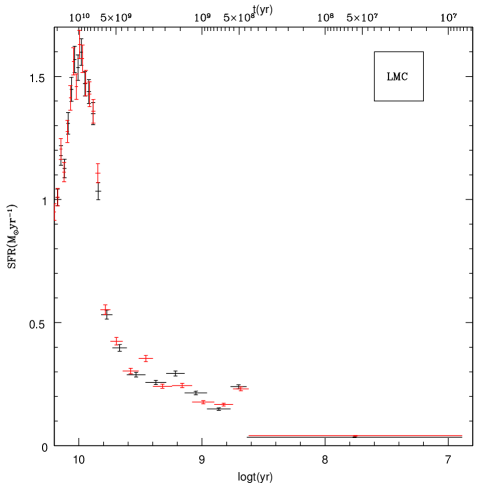
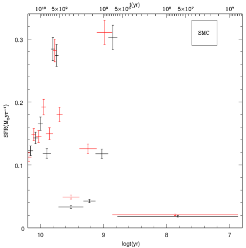
Figure 4: Global SFH of the LMC (left) and SMC (right) using both reddening correction approaches; black lines represent applying a carbonaceous-dust correction first, whilst red lines demonstrate the reverse (see Section 3.1.1). Vertical lines show statistical error bars described in Eq. (10). For the LMC, an initial burst of star formation as old as 10 Gyr is observed ($\log t=10$), with a SFR of $\sim 1.5$ M_⊙ yr^-1, followed by more quiescent star formation. In the case of the SMC, an initial burst of star formation as old as 6 Gyr is observed ($\log t=9.8$), with a SFR of $\sim 0.28$ M_⊙ yr^-1, followed by a secondary star formation epoch $\sim 0.7$ Gyr ago ($\log t=8.8$) with a SFR of $\sim 0.3$ M_⊙ yr^-1.

We thus derive the SFRs as a function of time, where we group the stars into bins of equal numbers – i.e., equal Poissonian significance. Figure 4 represents the SFHs for both reddening correction approaches (see Section 3.1.1); black lines indicate the case in which a carbonaceous-dust correction is first applied, and red lines demonstrate the reverse – however, there is no noticeable difference in the SFRs between these two correction approaches. Horizontal lines show time bins while vertical lines demonstrate statistical error bars derived as following;

$$\sigma_{\xi}\ =\ \frac{\sqrt{N}}{N}\ \xi,$$ (10)

where ”N” is the number of stars in each age bin. For the LMC (Fig. 4, left panel) we find an ancient star formation episode with rate of $1.598\pm 0.054$ M_⊙ yr^-1 $\sim 10$ Gyr ago ($\log t=10$), corresponding to the formation of the LMC: the total stellar mass produced in the LMC is $\sim 2.2\times 10^{10}$ M_⊙, of which $\approx 89$ per cent was formed during the first epoch. For the SMC (Fig. 4, right panel), two formation epochs are observed; one with a SFR of $0.282\pm 0.017$ M_⊙ yr^-1 rate $\sim 6$ Gyr ago ($\log t=9.8$) and a secondary star formation episode $\sim 0.7$ Gyr ago ($\log t=8.8$) with a similar SFR of $0.310\pm 0.019$ M_⊙ yr^-1. These findings are in good agreement with recent studies, e.g. Weisz et al. (2013). Of a total stellar mass in the SMC of $\sim 4.0\times 10^{8}$ M_⊙, $\approx 82$ per cent was produced during the first peak in SFR, and $\approx 11$ per cent during the second peak.

4.2 Star formation history of the central regions

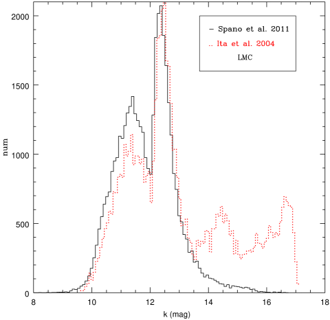
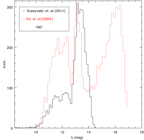
Figure 5: K-band histograms for variable stars in the overlapping regions (see Fig. 1) in the central parts of the LMC (left) and SMC (right), from Ita et al. (2004a) (red dotted lines), and from Spano et al. (2011) and Soszyński et al. (2011) (solid black lines) in the LMC and SMC, respectively. Each peak shows a type of variables, from left to right: AGB stars, RGB stars and Cepheids.

Before investigating the SFH in the central regions of the LMC and SMC, and comparing it to the SFH in their peripheries, we consider the use of the Ita et al. (2004a) catalogue for the central regions. Figure 5 shows the normalised K-band luminosity distributions. The peak at the brightest K-band magnitudes corresponds to the AGB; the second peak starts at $K\sim 12$ mag for the LMC and $K\sim 12.7$ mag for the SMC, which corresponds to the RGB tip. The deeper Ita et al. catalogue also contains fainter stars including Cepheids. For the purpose of our study, based mainly on AGB stars (and small numbers of RSGs) there is no indication that the IR catalogue of Ita et al. of the LMC variables offers any major advantage over the Spano et al. (2011) catalogue (we remind the reader that the latter is originally an optical catalogue cross matched with 2MASS). On the other hand, in the central part of the SMC, the Ita et al. catalogue is preferred over that of Soszyński et al. (2011) as the former is much more complete for the AGB stars.

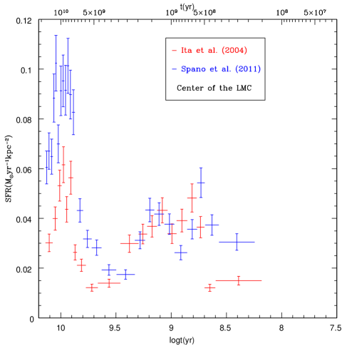
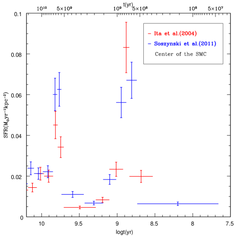
Figure 6: Left: SFH of the central bar structure in the LMC based on the catalogues of Ita et al. (2004a; red symbols) and Spano et al. (2011; blue symbols); along with statistical error bars discussed in Section 4.1. The Spano et al. data indicate a higher rate of initial star formation, by a factor of two compared to the Ita et al. data. However, the two data sets agree well on the more recent SFRs. Right: SFH of the overlapping region at the centre of the SMC based on the catalogues of Ita et al. (2004a; red symbols) and Soszyński et al. (2011; blue symbols). The Ita et al. data imply a higher rate of secondary star formation, whilst the Soszyński et al. data imply relatively higher rates during the initial star formation episode.

The SFH of the LMC was derived from the Ita et al. (2004a) catalogue, and for the overlapping region with the Spano catalogue (left panel in figure 6). This area corresponds to the bar structure of the LMC (see Fig. 1). For a meaningful comparison with the literature we report the SFR per physical area. The SFR in the LMC bar varies from $\sim 0.01$ to $0.1$ M_⊙ yr^-1 kpc^-2. Two formation epochs are seen; one epoch $\sim 10$ Gyr ago ($\log t=10$) when almost 48 per cent of the total stellar mass within the bar was formed, and a more recent epoch starting $\sim 3$ Gyr ago ($\log t=9.4$) which lasted until as recent as 500 Myr ago ($\log t=8.7$), within which almost 30 per cent of the total stellar mass was formed (the total stellar mass in the covered area is $\sim 1.4\times 10^{8}$ M_⊙). These two estimates are consistent between the use of both catalogues, except for the ancient epoch in which a higher SFR is found for the Spano data. However, it appears as though the SFR based on Spano et al. (2011) is more successful in recovering the ancient star formation. Cioni et al. (2014) also found the star formation history of the LMC using Vista survey of the Magellanic Clouds (VMC) which reported an old star formation at around $\log t=9.9$ as well as a secondary peak of star formation at $\sim\log t=8.5-8.7$ for stars closer to the LMC center. These two peaks in SFR coincide with the peaks that we have determined, though we argue for a more sustained star formation over the most recent few Gyr.

The SFH of the SMC based on the Ita et al. (2004a) catalogue was also derived and compared with that derived for the overlapping region in the Soszyński et al. (2011) catalogue (right panel in figure 6). This corresponds to the central, approximately square-degree region of the SMC (see Fig. 1). The SFR varies from $\sim 0.006$ M_⊙ yr^-1 kpc^-2 to $\sim 0.07$ M_⊙ yr^-1 kpc^-2. As in other studies (e.g., Cignoni et al. 2012), two formation episodes can be identified; one episode $\sim 6$ Gyr ago ($\log t=9.8$) when almost 49 per cent of the total stellar mass was formed, and another one $\sim 800$ Myr ago ($\log t=8.9$) within which around 12 per cent of the total stellar mass was formed. As for the LMC, the SFRs obtained for both catalogues agree rather well, however, the Ita et al. data indicate a relatively more pronounced secondary (recent) episode of star formation.

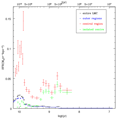
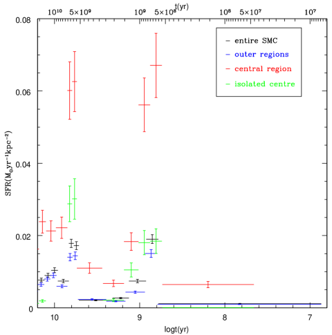
Figure 7: SFHs based on LPVs in the catalogues of Spano et al. (2011) for the LMC (left) and Soszyński et al. (2011) for the SMC (right). Black symbols: global star formation; blue symbols: star formation in the outskirt of the galaxies; red symbols: bar (for the LMC) and central (for the SMC) star formation; and green symbols: isolated star formation for the central regions derived by subtracting the SFH of the surrounding parts; along with statistical error bars explained in Section 4.1. For both galaxies, the bar/central star formation is remarkably dominant.

By excluding the stars in the bar/central regions of the galaxies (amounting to 3 deg² and 1 deg² in the LMC and SMC, respectively), we also obtained the SFH for the outer regions. Conversely, we also isolated the SFH of the bar/central regions by subtracting that derived for the immediately surrounding regions (which could also be seen in projection against and/or mixed with any distinct SFHs belonging to the bar/central regions). Figure 7 shows a comparison between the SFHs derived for the different regions. In case of the LMC, the second peak of star formation is not seen in the outer region whilst for the SMC, another remarkable peak of star formation is still observed in outer region. The latter is in good agreement with the work by Ripepi et al. (2014) who, using the optical STEP survey, found regions of high levels of star formation in the North and in the Wing of the SMC.

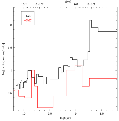
Figure 8: Ratio of the SFR in the centre compared to that in the outskirts, for the LMC (in black) and SMC (in red). Each bin in the histogram contains an equal number of stars. Clearly, star formation activity has been centrally concentrated in recent times, and possible always if old stars have migrated to the outskirts.

Figure 8 shows the ratio of the SFR in the central regions compared to that in the outer regions. Each bin in the histograms contain an equal number of stars. Note also the logarithmic scale. The LMC shows a steady concentration of younger stars in the central regions. A similar result was reported by Meschin et al. (2014), who found an ancient star formation epoch dating back 10 Gyr, followed by more recent star formation activity 4–1 Gyr ago. They also found younger stellar populations to be more centrally concentrated; in other words, the stellar population ages as one moves away from the center of the galaxy. Any such trend in the SMC is less obvious, though might also be present. Dynamical effects will have resulted in the migration of old stars towards the outskirts, so it is impossible to tell on the basis of this work whether star formation activity has always been centrally concentrated, or whether it has progressed further inwards as the galaxies matured. As the dynamical timescale is not much more than 100 Myr, stars that were formed more than a Gyr ago will have equilibrated their kinematics with the gravitational potential well – unless they have been exposed to recent tidal disturbances.

5 Concluding remarks

We find a significant difference in the ancient SFH of the LMC and the SMC. For the LMC, the bulk of the stars formed $\approx 10$ Gyr ago, while the strongest episode of star formation in the SMC occurred a few Gyr later. This is consistent with the findings of Weisz et al. (2013) obtained through CMD analysis of optical (Hubble space Telescope) photometry obtained in a few small regions in the centres and outskirts of the Magellanic Clouds. They argued that the relative enhancement in the SFH of the SMC is a consequence of the interaction with the LMC, with a stronger impact on the global star formation of the SMC due to its much smaller mass compared to the LMC. The smaller size of the SMC may also have resulted in the slower assembly at early times, similar to what was found in M 33 (Javadi et al. 2011). This would be easier to understand if the SMC and LMC did not form as a pair, but at least the SMC was formed in isolation.

A secondary peak of the SFH for the central part of the LMC has been reported in other studies, e.g., Smecker-Hane et al. (2001) who found a dominant star formation activity within the bar of the LMC at intermediate ages. Having isolated the SFH of the bar of the LMC from that of the disc, it has become clear that the bar formed a few Gyr ago and has maintained its star formation until very recently ($\sim 200$ Myr). However, the secondary peak in SFR in the SMC is much sharper (in duration) and occurred $\sim 700$ Myr ago. There is indeed a similar peak noticeable in the SFH of the LMC, and this is thus distinct from the star formation activity related to the bar itself. The co-eval 700-Myr bursts in the SMC and LMC are arguably due to the tidal interaction between the Magellanic Clouds and possibly their approach of the Milky Way (cf. Bekki & Chiba 2005; Indu & Subramaniam 2011).

Figure 9: Recent star formation of the Large Magellanic Cloud using Ulaczyk et al. (2013) catalogue of more massive (brighter) stars.

The LMC catalogues we have worked with are limited to $t\sim 100$ Myr due to the lack of more massive stars (brighter stars) because of saturation of the detectors used in the surveys. However, Ulaczyk et al. (2013) presented a catalogue of brighter stars that had been saturated in the main OGLE catalogue. On the basis of this bright sample we derive the recent SFH in the LMC using the methods described above (Fig. 9). We find a SFR of $\approx 0.19$ M_⊙ yr^-1 at $t\sim 5$ Myr, i.e. similar to that over the past Gyr or so (compare, for instance, with figure 4).

After applying a correction to the pulsation duration of LPVs as predicted by the stellar evolutionary models (see Javadi et al. 2013), the resulting SFRs are now in very good agreement with those obtained in other studies (e.g., Harris & Zaritsky 2004, 2009; Cignoni et al. 2012). However, a recent investigation by the Padova group of their own models revealed a severe over-estimation of the lifetimes of thermal-pulsing AGB stars (Girardi et al. 2013) which could also have implications for the duration of the radial pulsation phase. Indeed, the techniques we have pioneered in M 33 (Javadi et al. 2011, 2013), and now applied in the Magellanic Clouds, offer a promising avenue towards exposing the assembly and development of galaxies as well as improving models for the late stages of stellar evolution and mass loss.

References

- [Antoniou et al.(2010)] Antoniou V., Zezas A., Hatzidimitriou D., Kalogera V., 2010, ASPC, 424 ,230
- [Bekki et al.(2005)] Bekki K., Chiba M., 2005,MNRAS, 356, 680
- [Bekki (2012)] Bekki K., 2012, MNRAS, 422, 1957
- [Bertelli et al.(1992)] Bertelli G., Mateo M., Chiosi C., Bressan A., 1992, ApJ, 388, 400
- [Besla et al.(2012)] Besla G., Kallivayalil N., Hernquist L., van der Marel R.P., Cox T.J., Kereš D., 2012, MNRAS, 421, 2109
- [Cioni et al.(2006)] Cioni M.-R.L., Girardi L., Marigo P., Habing H.J., 2006, A&A, 448, 77
- [Cioni et al.(2014)] Cioni M.-R.L., et al., 2014, A&A, 562A, 32
- [Cignoni et al.(2012)] Cignoni M., et al., 2012, ApJ, 754, 130
- [Cignoni et al.(2013)] Cignoni M., et al., 2013, ApJ, 775, 83
- [Dolphin (1999)] Dolphin A.E., 1999, arXiv: 9910524v1
- [Freedman et al.(2010)] Freedman W.L., Kennicutt R.C., Mould J.R., 2010, HiA, 15, 1
- [Gieren et al.(2005)] Gieren W., et al., 2005, ApJ, 627, 224
- [Girardi et al.(2013)] Girardi L., Marigo P., Bressan A., Rosenfield P., 2013, ApJ, 777, 142
- [Glatt et al.(2010)] Glatt K., Grebel E.K., Koch A., 2010, A&A, 517, 50
- [Harris & Zaritsky,(2004)] Harris J., Zaritsky D., 2004, AJ, 127, 1531
- [Harris & Zaritsky (2009)] Harris J., Zaritsky D., 2009, AJ, 138, 1243
- [Haschke et al.(2011)] Haschke R., Grebel E.K., Duffau S., 2011, AJ, 141, 1865
- [Holtzman et al.(1999)] Holtzman J.A., et al., 1999, AJ, 118, 2262
- [Indu & Subramaniam (2011)] Indu G., Subramaniam A., 2011, A&A, 535, A115
- [Ita et al.(2004a)] Ita Y., et al., 2004a, MNRAS, 347, 720
- [Ita Y., et al.(2004ab)] Ita Y., et al., 2004b, MNRAS, 353, 705
- [Javadi et al.(2011)] Javadi A., van Loon J.Th., Mirtorabi M.T., 2011, MNRAS, 414, 3394
- [Javadi et al.(2013)] Javadi A., van Loon J. Th., Khosroshahi H., Mirtorabi M., 2013, MNRAS, 432, 2824
- [Kerber et al.(2009)] Kerber L.O., Girardi L., Rubele S., Cioni M.-R.L., 2009, A&A, 499, 697
- [Luri et al.(1998)] Luri X., Gomez A.E., Torra J., Figueras F., Mennessier M.O., 1998, A&A, 335, 81
- [Macri et al.(2006)] Macri L.M., Stanek K.Z., Bersier D., Greenhill L.J., Reid M.J., 2006, ApJ, 652, 1133
- [Marigo et al.(2008)] Marigo P., Girardi L., Bressan A., Groenewegen M.A.T., Silva L., Granato G.L., 2008, A&A, 482, 883
- [Maschberger & Kroupa (2011)] Maschberger T., Kroupa P., 2011, MNRAS, 411, 1495
- [Meschin et al.(2014)] Meschin I., et al., 2014, MNRAS, 438, 1067
- [Monelli et al.(2011)] Monelli M., et al., 2011, EAS, 48, 43
- [Nanni et al.(2013)] Nanni A., Bressan A., Marigo P., Girardi L., 2013, MNRAS, 434, 2390
- [Nidever et al.(2011)] Nidever D.L., et al., 2011, ApJ, 733, L10
- [Ripepi et al.(2014)] Ripepi V., et al., 2014, MNRAS, 442, 1897
- [Rubele et al.(2011)] Rubele S., Girardi L., Kozhurina-Platais V., Goudfrooij P., Kerber L., 2011, MNRAS, 414, 2204
- [Rubele et al.(2013)] Rubele S., et al., 2013, MNRAS, 430, 2774
- [Smecker-Hane et al.(2002)] Smecker-Hane T.A., Cole A., Gallagher J.S., Stetson P., 2002, ApJ, 566, 239
- [Soszyński et al.(2011)] Soszyński I., et al., 2011, AcA, 61, 217
- [Spano et al.(2011)] Spano M., et al., 2011, A&A, 536 A, 60
- [Subramanian & Subramaniam (2011)] Subramanian S., Subramaniam A., 2011, ASInC, 3, 144
- [Ulaczyk et al.(2013)] Ulaczyk K., et al., 2013, AcA, 63, 159
- [van Loon et al.(1997)] van Loon J.Th., Zijlstra A.A., Whitelock P.A., Waters L.B.F.M., Loup C., Trams N.R., 1997, A&A, 325, 585
- [van Loon et al.(2008)] van Loon J.Th., et al., 2008, A&A, 487, 1055
- [van Loon et al.(2010)] van Loon J.Th., Oliveira J.M., Gordon K.D., Sloan G.C., Engelbracht C.W., 2010, AJ, 139, 1553
- [Weisz et al.(2013)] Weisz D.R., et al., 2013, MNRAS, 431, 364
- [Whitelock et al.(2003)] Whitelock P.A., Feast M.W., van Loon J.Th., Zijlstra A.A., 2003, MNRAS, 342, 86
- [Wood et al.(1992)] Wood P.R., Whiteoak J.B., Hughes S.M.G., Bessell M.S., Gardner F.F., Hyland A.R., 1992, ApJ, 397, 552