Effective ergodicity breaking in an exclusion process with varying system length

Abstract

Stochastic processes of interacting particles in systems with varying length are relevant e.g. for several biological applications. We try to explore what kind of new physical effects one can expect in such systems. As an example, we extend the exclusive queueing process that can be viewed as a one-dimensional exclusion process with varying length, by introducing Langmuir kinetics. This process can be interpreted as an effective model for a queue that interacts with other queues by allowing incoming and leaving of customers in the bulk. We find surprising indications for breaking of ergodicity in a certain parameter regime, where the asymptotic growth behavior depends on the initial length. We show that a random walk with site-dependent hopping probabilities exhibits qualitatively the same behavior.

I Introduction

The exclusive queueing process (EQP) bib:A ; bib:YTJN ; bib:AY ; bib:ASPED14 ; bib:M3AS is a queueing model that takes into account the spatial structure of the queue. In standard queueing theory, which is a well-established approach of practical relevance bib:E ; bib:K ; bib:Sa , the system length and the number of particles are identical, so that the density along the queue is always 1. In the EQP, particles interact with each other through an exclusion principle, i.e. they can move forward only when the target site is empty. Thus the density is not a constant. The EQP is equivalent to the totally asymmetric simple exclusion process (TASEP) bib:L ; bib:Schuetz ; bib:CSS ; bib:SCN of varying length. One end of the chain is fixed and corresponds to the server to which particles move. Arriving particles always join the queue at the site just behind the opposite end of the queue. In earlier works bib:AY ; bib:AS1 the phase diagram of the EQP with parallel update scheme has been determined exactly. It shows two main phases that correspond to queues with converging and diverging lengths. These phases can further be divided into several subphases, see bib:AS1 ; bib:AS2 ; bib:AS3 for details.

In the previous work bib:AS4 , unusual critical behavior of the EQP has been observed. This indicates that dynamical systems of fluctuating length might show surprising properties. Due to the relevance of stochastic processes with varying system length, in particular for applications to biology bib:SEPR ; bib:SE ; bib:ES ; bib:DMP ; bib:JEK ; bib:MRF ; bib:SS ; bib:M ; bib:dGF , it is worthwhile to explore them in more detail. Extending our previous works, here we introduce an EQP with Langmuir kinetics (EQP-LK) that allows creation and annihilation of particles anywhere in the bulk of the queue, not only at the ends. This can be interpreted as an effective model for interacting queues. For customer queues, customers might change to (from) the bulk of the queue from (to) other queues. Looking at a specific queue this has the same effects as Langmuir kinetics characterized by a detachment probability $\omega_{D}$ and an attachment probability $\omega_{A}$ (if every vacancy in the queue can be occupied by an arriving customer).

In this work, we shall characterize the EQP-LK via the system length $L_{t}$ at time $t$. We begin by introducing a naive test to determine whether the system length diverges or converges to a stationary length by averaging simulation samples with initial condition $L_{t=0}=0$. Next we shall examine the time evolution of the average system length $\langle L_{t}\rangle$. Surprisingly its behavior depends on the initial system length $L_{0}=L_{t=0}$, indicating the breaking of ergodicity. Furthermore, we shall see that individual simulation samples can exhibit different behaviors. We shall qualitatively explain these unexpected phenomena by constructing a random walk model which captures the essential features of the length dynamics. We expect that these new insights could be of relevance also for the interpretation of experimental studies on systems of varying length, especially in biology.

II Model

The model that we study is a combination of the EQP with parallel update bib:AY and Langmuir kinetics (EQP-LK), see Fig. 1. It is defined on a semi-infinite one-dimensional lattice, where the sites are numbered from right to left. Each site $j\in\mathbb{N}$ is either occupied by a particle ($\tau_{j}=1$) or empty ($\tau_{j}=0$). Our model’s state space is infinite but countable, consisting of configurations $\tau_{L}\cdots\tau_{1}$ and a state $\emptyset$ where there is no particle. The system length $L$ is defined by the leftmost occupied site or $L=0$ for the state $\emptyset$. The system length is, in general, different from the number of particles, in contrast to classical queueing models. Particles move forward (rightward in Fig. 1) with probability $p$ in each time step only if the preceding site is unoccupied. A new particle enters at the end of the queue (i.e. $j=L+1$) with probability $\alpha$. When there is no particle in the system, a new particle enters directly at site $j=1$. Particles in the bulk are detached with probability $\omega_{D}$, and for each empty site $j(\leq L)$ a particle is attached with probability $\omega_{A}$. As in the TASEP with Langmuir kinetics (TASEP-LK) bib:PFF ; bib:Popkov ; bib:EJS ; bib:DG , the attachment and detachment probabilities are scaled with the system length as $\omega_{A}=\Omega_{A}/L$ and $\omega_{D}=\Omega_{D}/L$. The total probabilites $\Omega_{A}$ and $\Omega_{D}$ are kept constant. Then inflow and outflow caused by the Langmuir kinetics are given by $(1-\rho)\Omega_{A}$ and $\rho\Omega_{D}$, where $\rho$ is the global density of the system. It is of the same order of magnitude as the boundary currents so that the dynamics of the system is determined by a competition between bulk and boundary dynamics. In contrast to the TASEP-LK, the system length $L$ of the EQP-LK varies, and thus the probabilities $\omega_{A},\omega_{D}$ depend on the current state and thus has to be determined from the fixed values of $\Omega_{A},\Omega_{D}$ as $\omega_{A}=\Omega_{A}/L$ and $\omega_{D}=\Omega_{D}/L$. In each time step, first the configuration is updated according to the rule of the EQP with parallel update, and then the Langmuir kinetics is applied. This defines the EQP-LK with parameters $(p,\alpha,\beta,\Omega_{A},\Omega_{D})$, which is generically an irreducible and aperiodic discrete-time Markov process. We denote by $L_{t}$ the system length at time $t$ for a realization (a simulation run) of the stochastic process and by $\langle L_{t}\rangle$ its average over different realizations.

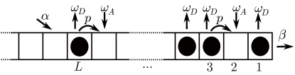
Figure 1: Transition probabilities of the exclusive queueing process with Langmuir kinetics (EQP-LK).

III Phase diagram

First we revisit the EQP with parallel update, corresponding to the special case of the EQP-LK with $\Omega_{A}=\Omega_{D}=0$. The parameter space is divided into two regimes by the “critical line”

$$\alpha_{c}=\begin{cases}\beta(p-\beta)/(p-\beta^{2})&(\text{for }\beta\leq 1-\sqrt{1-p}),\\ (1-\sqrt{1-p})/2&(\text{for }\beta>1-\sqrt{1-p}).\end{cases}$$ (1)

For $\alpha<\alpha_{c}$ (“convergent phase”), the average length $\langle L_{t}\rangle$ converges to a stationary value. On the other hand, for $\alpha>\alpha_{c}$ (“divergent phase”), $\langle L_{t}\rangle$ diverges. These properties were shown rigorously by constructing an exact stationary distribution bib:AY . Furthermore, in the divergent phase, the asymptotic behavior of $\langle L_{t}\rangle$ was shown to be linear in time $\langle L_{t}\rangle=Vt$ with an explicit form for the velocity $V$, by simulations for general $p$ bib:AS3 and by using an exact time-dependent solution for $p=1$ bib:AS2 .

Now we introduce a test to distinguish between diverging and converging system lengths by simulations. Starting from $L_{t=0}=0$, the quantity

$$R_{T}=\sum_{3T/4<t\leq T}\langle L_{t}\rangle\big{/}\sum_{T/2<t\leq 3T/4}\langle L_{t}\rangle$$ (2)

approaches $R_{\text{conv}}=1$ as $T\to\infty$ in the convergent phase. On the other hand, if we assume $\langle L_{t}\rangle$ diverges linearly in time, the quantity $R_{T}$ approaches $R_{\text{div}}=7/5$. In computer simulations only finite $T$ can be studied. Here we set $T=2\cdot 10^{4}$. Averages are calculated with a finite number $10^{3}$ of samples. The phase transition is identified as the point where $R$ becomes bigger than the average

$$R_{T}>(R_{\text{conv}}+R_{\text{div}})/2=6/5$$ (3)

when $\alpha$ is increased with the other parameters fixed. In Fig. 2(a), we observe that for the EQP the critical line obtained by this test agrees with the exact line.

Let us apply the test to the EQP-LK, again starting from the initial state $\emptyset$. The phase boundary between the two phases depends on the Langmuir probabilities $\Omega_{A}$ and $\Omega_{D}$, see Fig. 2. When the ratio $\Omega_{A}/\Omega_{D}$ is 1, we observe that the phase boundary becomes simply a straight segment $\alpha=(1-\sqrt{1-p})/2$ as $\Omega_{A}=\Omega_{D}\to 1$, see Fig. 2 (a). For fixed $\Omega_{D}$, the natural observation is that the convergent phase is enlarged for increasing values of $\Omega_{A}$, see Fig. 2 (b), (c) and (d). Again the critical line becomes a straight segment (which is independent of $\alpha$) as $\Omega_{D}$ increases.

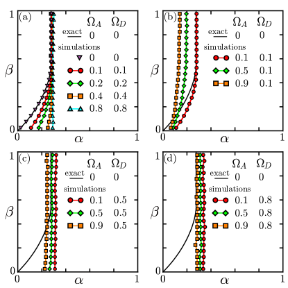
Figure 2: Phase diagrams for various values of $\Omega_{D},\Omega_{A}$ and $p=0.8$, determined by the test (3). For comparison, the exact critical line (1) for the EQP case $\Omega_{D}=\Omega_{A}=0$ is shown, which is recovered by the test.

IV Dependence on initial conditions

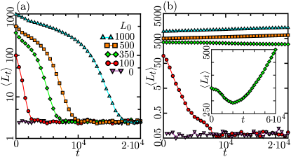
Figure 3: Behavior of $\langle L_{t}\rangle$ starting from various initial lengths, for the parameters given in Eqn. (4)(a) and Eqn. (5)(b). We have set the initial density as $\Omega_{A}/(\Omega_{D}+\Omega_{A})$, and averaged over $10^{3}$ samples. In (a), all the average lengths ($L_{0}=0,100,350,500,1000$) converge to a stationary value. In (b), we observe not all the average lengths converge.

The EQP-LK with generic values of parameters is an irreducible and aperiodic Markov process on a countable state space. The general theory of Markov processes bib:Schinazi tells us that the convergence of $\langle L_{t}\rangle$ is independent of the initial state. We now check this property by simulations. For example, the case

$$(p,\alpha,\beta,\Omega_{A},\Omega_{D})=(0.8,0.2,0.2,0.2,0.35)$$ (4)

is determined to be in the convergent phase by the test (3). In fact, the average lengths $\langle L_{t}\rangle$ over $10^{3}$ simulation samples with other initial lengths $L_{0}$ converge to the same stationary value, see Fig. 3(a). Surprisingly, however, this is not always true. For example, for

$$(p,\alpha,\beta,\Omega_{A},\Omega_{D})=(0.8,0.3,0.2,0.1,0.9),$$ (5)

the average length $\langle L_{t}\rangle$ with $L_{0}=0$ converges but the average lengths with large initial lengths (e.g. $L_{0}=500,1000$) do not converge, see Fig. 3(b). Furthermore, starting from an intermediate length (e.g. $L_{0}=350$), the average length $\langle L_{t}\rangle$ exhibits a non-monotonic behavior. In the inset of Fig. 3 (b), $\langle L_{t}\rangle$ decreases until $t\sim 2\cdot 10^{4}$ and then increases. In the rest of this work, we shall try to understand this unexpected phenomenon with the specific set of parameter values (5). We emphasize that this unexpected behavior is observed generically in a larger parameter regime BA1 ; BA2 .

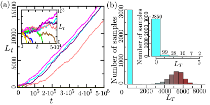
Figure 4: (a) Behaviors of $L_{t}$ for 9 individual samples and (b) the length distribution of $5\cdot 10^{3}$ samples at time $t=T=2\cdot 10^{5}$. The parameters were set as Eqn. (5), and every sample started from the length $L_{0}=350$ and the density $\Omega_{A}/(\Omega_{A}+\Omega_{D})=0.1$. More precisely, the bars in (b) represent the number of samples that satisfy $L_{T}\in[0,500),[500,1000),\ldots$. The inset shows more detailed distribution near $L_{T}=0$, i.e. the bars represent the numbers of samples such that $L_{T}=0,1,\ldots,5$.

First, let us investigate the behavior of individual samples. Comparing the insets of Fig. 3(b) and Fig. 4(a), we notice that the individual behaviors do not perfectly mimic the behavior of the average. In other words, the average does not represent the typical behavior of individual samples. Therefore the dynamics of the system cannot be properly understood by just looking at averages. For example, on the “coexistence line” of the TASEP with open boundaries, the average density profile is linear. However, this does not imply that a shock is moving, which can only be observed for individual samples bib:KSKS .

In Fig. 4(a), we observe that 5 of 9 samples hit $L_{t}=0$ within $t<5\cdot 10^{4}$. We call them converging samples. The other 4 samples increase almost linearly in time, even after $t\sim 10^{5}$ (diverging samples). Let us look at statistics of $5\cdot 10^{3}$ samples with the same parameter setting and the same initial length [Fig. 4(b)]. Apparently there are two peaks at $L_{T}\in[0,500)$ and $L_{T}\in[5000,5500)$, corresponding to converging and diverging samples, respectively. Because of the strong effect of the detachment $\Omega_{D}=0.9$, it is difficult to escape from $L_{t}=0$ after reaching $L_{t}=0$, see the inset of in Fig. 4(b). The non-monotonicity observed for the average $\langle L_{t}\rangle$ is due to the dominance of the contributions from the diverging samples whereas the contribution of the converging can be neglected once they have reached $L_{t}=0$. We note that $L_{t}=0$ is not an absorbing state, and our model exhibits no absorbing transition which was studied in a symmetric exclusion process with varying length bib:BH .

Distributions of simulation samples for various initial lengths is provided in Fig. 5(a,b). We observe that the samples starting from a short queue tend to remain short. More samples starting from a long queue tend to grow. The growth of each of them is almost proportional to time $t$ as well as their average, see Fig. 4(a) and Fig. 5(c).

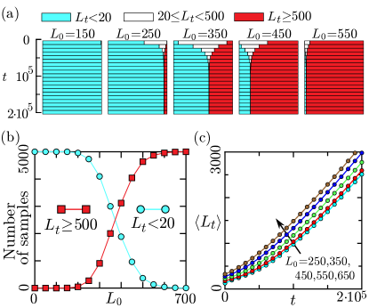
Figure 5: (a,b) System length $L_{t}$ distributions of $5\cdot 10^{3}$ simulation samples, and (b) behavior of $L_{t}$ averaged over diverging samples, with parameters (5). The samples started from various initial lengths at density $\Omega_{A}/(\Omega_{A}+\Omega_{D})=0.1$. In (a) the samples are divided into three groups according to $L_{t}\in[0,20),[20,500)$ or $[500,\infty)$ at time $t=10^{4},2\cdot 10^{4},3\cdot 10^{4},\dots,2\cdot 10^{5}$. The lengths of bands represent the ratio of the number of samples classified into each group. The plots of the number of samples at $t=2\cdot 10^{5}$ are given in (b). The plots in (c) are given by averaging over samples that have never hit $L_{t}=0$ within $t\leq 2\cdot 10^{5}$.

V First passage time

Let us consider the first passage time bib:R , i.e. the first time $h$ when a sample hits the length $L_{h}=L$, starting from $L_{0}=0$. We observe that the average first passage time becomes very large as $L$ increases [Fig. 6 (a)], and it seems to increase faster than power law. Thus it is impossible to reach e.g. $L_{t}=500$ in our computer simulations, even though the probability of ever hitting the length $L_{t}=500$ is 1. In this sense, the ergodicity of the EQP-LK is effectively broken. The difficulty of reaching $L_{t}=500$ is also implied by Fig. 6 (b), where the average first passage time becomes extremely large as $\alpha$ decreases.

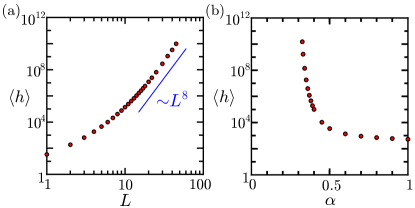
Figure 6: (a) Mean first passage time $\langle h\rangle$ (when samples visit $L_{h}=L$ for the first time) vs $L$. The parameters were chosen as in Eqn. (5) with initial length $L_{0}=0$. Averages were taken over $10^{4}$ (for $L\leq 30$) or $500$ (for $L>30$) simulation samples. For comparison the line const.$\times L^{8}$ is shown. (b) Mean first passage time $\langle h\rangle$ when samples visit $L_{h}=500$ for the first time vs $\alpha$. The other parameters were chosen as $(p,\beta,\Omega_{A},\Omega_{D})=(0.8,0.2,0.1,0.9)$. Averages were taken over $10^{4}$ (for $\alpha\geq 0.35$), $10^{2}$ (for $\alpha=0.33,0.34$) or $10$ (for $\alpha=0.325$) simulation samples.

VI Random walk model

The mechanism underlying the effective ergodicity breaking can be qualitatively understood in terms of a random walk model. The position of the walker corresponds to the system length $L$ and the random walk has one reflecting end corresponding to $L=0$. We denote the hopping probabilities by $q_{L}$ for $L\to L+1$ and by $r_{L}$ for $L+1\to L$. The behavior of the length of the EQP-LK can be qualitatively modeled by hopping probabilities that satisfy

$$\frac{q_{L}}{r_{L}}\begin{cases}<1&(L<L^{*}),\\ =1&(L=L^{*}),\\ >1&(L>L^{*})\end{cases}$$ (6)

with some $L^{*}$. In other words, the potential bib:RPS $U(L)=\sum_{j=0}^{L-1}\ln\frac{r_{j}}{q_{j}}$ takes a maximum at $L=L^{*}$, and $\lim_{L\to\infty}U(L)=-\infty$, see Fig. 7. One of the simplest examples is the case where $q_{L}=1-r_{L-1}=\frac{1}{2\pi}\arctan(\frac{L-L^{*}}{c})+\frac{1}{2}$ with some $c$.

The walker tends to move towards $L=0$ when it is on a position $L<L^{*}$. Oppositely a walker on $L>L^{*}$ tends to move towards $L=+\infty$. This inhomogeneous bias corresponds to the length dependence of the Langmuir probability; when the system length is short, a newly entering particle at the left end, which would increase the length, can easily be removed. On the other hand, in a long queue this effect is weak since $\Omega_{D}/L\approx 0$. Therefore the initial condition and initial behavior are very important. Once the walker reaches $L=0$, it cannot easily escape. It then fluctuates near $L=0$, but this is not a true stationary state. We remark that one can easily prove that there is no stationary distribution, and the walker’s position should diverge in the long-time limit. Thus the random walk model exhibits qualitatively the same behavior as observed in the EQP-LK (see Figs. 4 and 5).

Figure 7: An inhomogeneous random walk model with one reflecting boundary (at $L=0$). When the walker is on a position $L<L^{*}$ ($L>L^{*}$), it prefers to go to $L=0$ (resp. $L=+\infty$).

VII Discussion

We have analyzed a queueing model with excluded-volume effect and Langmuir kinetics by simulations. Due to the varying length of the system, the Langmuir probabilities depend on the current state in each simulation run, which has a significant influence on the dynamics, e.g. a strong dependence on the initial condition and effective ergodicity breaking. There is a phase where long queues ($L>L^{*}$) prefer to grow, whereas short queues ($L<L^{*}$) prefer to remain short, although full identification of such regime has not yet been completed BA1 ; BA2 .

The EQP-LK shows that stochastic systems on fluctuating geometries can exhibit surprising behavior. We believe that beyond the theoretical interest our findings could be relevant for the interpretation of experimental (where the number of samples is necessarily finite) results as well, especially in biological systems.

Acknowledgements:
We are grateful to Christian Borghardt for his contributions in an early stage of this work. We also thank Martin R. Evans and Joachim Krug for useful discussions. This work was partially supported by Deutsche Forschungsgemeinschaft (DFG) under grant “Scha 636/8-1”.

References

- (1) C. Arita, Phys. Rev. E 80, 051119 (2009)
- (2) D. Yanagisawa, A. Tomoeda, R. Jiang and K. Nishinari, JSIAM Lett. 2, 61 (2010)
- (3) C. Arita and D. Yanagisawa, J. Stat. Phys. 141, 829 (2010)
- (4) C. Arita and A. Schadschneider, Transp. Res. Proc. 2, 87 (2014)
- (5) C. Arita and A. Schadschneider, Math. Models Meth. Appl. Sci. 25, 401 (2015)
- (6) A. K. Erlang, Nyt. Tidsskr. Mat. Ser. B 20, 33 (1909)
- (7) D. G. Kendall, J. Roy. Statist. Soc. Ser. B 13 (2), 151 (1951)
- (8) T. L. Saaty, Elements of Queueing Theory With Applications, Dover Publ. (1961)
- (9) T. M. Liggett, Stochastic Interacting Systems: Contact, Voter and Exclusion Processes, Springer, New York (1999)
- (10) G. M. Schütz, in Phase Transitions and Critical Phenomena, Vol. 19, C. Domb and J. L. Lebowitz (Eds.), Academic Press, San Diego (2001)
- (11) D. Chowdhury, L. Santen and A. Schadschneider, Phys. Rep. 329, 199 (2000)
- (12) A. Schadschneider, D. Chowdhury and K. Nishinari, Stochastic Transport in Complex Systems: From Molecules to Vehicles, Elsevier Science, Amsterdam (2010)
- (13) C. Arita and A. Schadschneider, Phys. Rev. E 83, 051128 (2011)
- (14) C. Arita and A. Schadschneider, Phys. Rev. E 84, 051127 (2011)
- (15) C. Arita and A. Schadschneider, J. Stat. Mech. (2012) P12004
- (16) C. Arita and A. Schadschneider, EPL 104, 30004 (2013)
- (17) K. E. P. Sugden, M. R. Evans, W. C. K. Poon and N. D. Read, Phys. Rev. E 75, 031909 (2007)
- (18) K. E. P. Sugden and M. R. Evans, J. Stat. Mech. (2007) P11013
- (19) M. R. Evans and K. E. P. Sugden, Physica A 384, 53 (2007)
- (20) S. Dorosz, S. Mukherjee and T. Platini, Phys. Rev. E 81, 042101 (2010)
- (21) D. Johann, C. Erlenkämper and K. Kruse, Phys. Rev. Lett. 108, 258103 (2012)
- (22) A. Melbinger, L. Reese and E. Frey, Phys. Rev. Lett. 108, 258104 (2012)
- (23) M. Schmitt and H. Stark, EPL 96 28001 (2011)
- (24) S. Muhuri, EPL 101, 38001 (2013)
- (25) J. de Gier and C. Finn, J. Stat. Mech. (2014) P07014
- (26) A. Parmeggiani, T. Franosch, E. Frey, Phys. Rev. Lett. 90, 086601 (2003)
- (27) V. Popkov, A. Rakos, R.D. Willmann, A.B. Kolomeisky, G.M. Schütz, Phys. Rev. E 67, 066117 (2003)
- (28) M. R. Evans, R. Juhasz, L. Santen, Phys. Rev. E 68, 026117 (2003)
- (29) I. Dhiman, A. K. Gupta, EPL 107, 20007 (2014)
- (30) R. B. Schinazi, Classical and Spatial Stochastic Process, Birkhäuser, Boston (1999)
- (31) C. Schultens, Bachelor Thesis, University of Cologne (2012)
- (32) C. Borghardt, Bachelor Thesis, University of Cologne (2012)
- (33) A. B. Kolomeisky, G. M. Schütz, E.B. Kolomeisky and J. P. Straley, J. Phys. A: Math. Gen. 31, 6911 (1998)
- (34) A. C. Barato and H. Hinrichsen, Phys. Rev. Lett. 100, 165701 (2008)
- (35) S. Redner, A Guide to First-Passage Processes, Cambridge University Press, Cambridge (2007)
- (36) A. Rákos, M. Paessens, and G. M. Schütz, Phys. Rev. Lett. 91, 238302 (2003)
- (37) F. Zielen, A. Schadschneider, Phys. Rev. Lett. 89, 090601 (2002)